the Creative Commons Attribution 3.0 License.
the Creative Commons Attribution 3.0 License.
Multiconfiguration electromagnetic induction survey for paleochannel internal structure imaging: a case study in the alluvial plain of the River Seine, France
Fayçal Rejiba
Cyril Schamper
Antoine Chevalier
Benoit Deleplancque
Gaghik Hovhannissian
Julien Thiesson
Pierre Weill
The La Bassée floodplain area is a large groundwater reservoir controlling most of the water exchanged between local aquifers and hydrographic networks within the Seine River basin (France). Preferential flows depend essentially on the heterogeneity of alluvial plain infilling, whose characteristics are strongly influenced by the presence of mud plugs (paleomeander clayey infilling). These mud plugs strongly contrast with the coarse sand material that composes most of the alluvial plain, and can create permeability barriers to groundwater flows. A detailed knowledge of the global and internal geometry of such paleomeanders can thus lead to a comprehensive understanding of the long-term hydrogeological processes of the alluvial plain. A geophysical survey based on the use of electromagnetic induction was performed on a wide paleomeander, situated close to the city of Nogent-sur-Seine in France. In the present study we assess the advantages of combining several spatial offsets, together with both vertical and horizontal dipole orientations (six apparent conductivities), thereby mapping not only the spatial distribution of the paleomeander derived from lidar data but also its vertical extent and internal variability.


Dipolar source electromagnetic induction (EMI) techniques are frequently used for critical zone mapping, which can be applied to the delineation of shallow heterogeneities, thereby improving conceptual models used to explain the processes affecting a wide range of sedimentary environments. This mapping technique is very effective for environments in which the spatial structure has strongly contrasted electromagnetic (EM) properties – especially that of interpreted electrical conductivity (EC).
Since the seminal work of Rhoades et al. (1976) much research has been conducted to link the petrophysical and hydrodynamic soil properties to the apparent electrical conductivity (ECa). ECa is affected by numerous parameters (Friedman, 2005) whose major ones can be separated into three categories: (1) the bulk soil properties (porosity, water content, structure), (2) the type of solid particle (geometry, distribution and cation exchange capacity) mainly related to the clay content, and (3) environmental factors (EC of water, temperature, etc.). The clay infilling of paleochannels and the deposition of alternate layers of conductive (clayey) and resistive (sandy) material in alluvial plain systems are examples of natural geophysical processes having contrasting EM properties.
EMI measurements have previously been applied to the imaging of conductive fine-grained paleomeander infilling, produced by meander neck cutoff or river avulsion, which can form permeability barriers with complex geometries (e.g. Miall, 1988; Fitterman et al., 1991; Jordan and Prior, 1992; De Smedt et al., 2011). In addition to providing detailed local information on alluvial plain heterogeneities, which can be applied to the study of aquifer–river exchanges (Flipo et al., 2014), the estimation of the geometry of the Seine River paleochannels can provide valuable insight into its paleohydrology, as well as physical transformations resulting from climatic fluctuations during the Late Quaternary.
EMI devices are increasingly used for a large number of near-surface geophysical applications, as a consequence of their ability to produce mapping of ECa over extended areas and at different depths. The main issue of EMI concerns the quantitative mapping of the vertical variations of EC, obtained after multilayer inversion of ECa, because of the limited number of measurements at different depths (i.e. source–receiver offsets). Despite the spreading use of multiple-frequency and multiple-coil EMI instruments compared to the classic twin-coil configuration, a way to overcome this issue is, at least to constrain, and at best to calibrate multilayer inversion of EMI measurements against ERI (electrical resistivity imagery) profiling. A very large body of scientific literature has been published on the study and use of near-surface electromagnetic geophysics, especially in the frequency domain, as described by Everett (2012).
By design, an EMI system energizes a transmitter coil with a monochromatic oscillating current, and the oscillating magnetic field produced by this current induces an oscillating voltage response in the receiver coil. The voltage response measured in the absence of any conductive structure is used as a standard reference. However, the magnetic field oscillations are distorted by the presence of nearby conductive structures, such that the voltage signal induced in the receiver coil experiences a shift in amplitude and phase with respect to that observed in the standard reference. This shift can be conveniently represented by a complex number, comprising quadrature (or imaginary) and in-phase (or real) components, which can be interpreted in terms of ECa (from the quadrature or out-of-phase part) and depth of investigation (DOI) (Huang, 2005). A comprehensive and more detailed description of the EMI principles can be found in Nabighian (1988a, b).
Although EMI systems were initially used as mapping tools, and were designed to measure the lateral variability of EC associated with a single DOI, the measurements they provide are now generally interpreted to provide information as a function of depth, albeit down to only relatively shallow depths. This interpretation relies on the fact that, for a given soil model, one specific DOI is defined by four device setup parameters: (1) the offset between the transmitter and receiver magnetic dipole, (2) the orientation of the dipole pair, (3) the frequency of the transmitter current oscillations, and (4) the instrument height above the ground. An EMI survey during which at least one of these parameters is varied can thus be used to resolve depth-related variations of EC. This distribution can be retrieved by solving an inverse problem, which is derived from a large number of applications (e.g. Tabbagh, 1986; Nabighian, 1988b; Spies, 1989; Schamper et al., 2012).
The physical model used in the inversion procedure must be suitably adapted to the electromagnetic properties of the surveyed ground. In the case of a medium characterized by typical conductive properties (e.g. low, non-ferromagnetic materials), at a low induction number the quadrature response is interpreted in terms of the apparent ground resistivity, which to a first-order approximation varies linearly with the quadrature response (McNeill, 1980). In a resistive (EM effects other than induction become non negligible) or highly conductive (low-induction number assumption is no longer valid) environment, such as that mapped in the present study, the EMI recordings, in particular their in-phase component, must be interpreted within the specific measurement context. One must then take into account, in addition to the EC, the magnetic susceptibility and viscosity, as well as the dielectric permittivity of the local environment, especially if this is resistive (e.g. Simon et al., 2015; Benech et al., 2016).
The present study focuses on the La Bassée alluvial plain, a zone located in the southern part of the Seine Basin, 2 km to the west of Nogent-sur-Seine (France). The geophysical campaign was performed during 3 days of good weather in June during a low-water period. The use of geophysical exploration for this investigation is of significant importance, since it should pave the way for the paleohydrological reconstruction of the Seine River (estimation of its transversal geometry and paleo-discharge).
The aim of this study is to delineate the geometry of a paleochannel (i.e. its thickness and width), using a state-of-the-art 1-D inversion routine applied to EMI ECa measurements. The inverted data consist in a set of EMI measurements implemented with (1) three different offsets, and (2) for two dipole configurations: horizontal (HCP) and vertical (VCP).
Following a description of the study area, we present the technique used to calibrate the EMI measurements, which relies on reference ERI (electrical resistivity imaging) measurements and an auger sounding profile. The EMI inversion is then constrained to limit the solution space to images that are consistent with the observations provided by the ERI and auger soundings. To this end, a local three-layer model is derived with fixed conductivities, and is then introduced into the inversion routine for each position of the surveyed area. The thicknesses of the soil and conductive filling, corresponding to the presumed paleochannel, are determined through the use of an inversion algorithm.
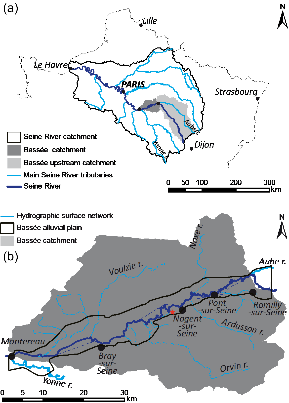
The study site is located within a portion of the Seine River alluvial plain (locally named “Bassée”), approximately one hundred kilometres upstream of Paris (France), between the confluence of the Seine and Aube rivers to the northeast, and the confluence of the Seine and Yonne rivers to the southwest (Fig. 1). This 60 km long, 4 km wide alluvial plain constitutes a heterogeneous sedimentary environment, resulting from the development of the Seine River during the Middle and Late Quaternary.
Cartographic studies of this area have been carried out in the past, using geomorphological and sedimentological techniques (Mégnien, 1965; Caillol et al., 1977; Mordant, 1992; Berger et al., 1995; Deleplancque, 2016), thus allowing the broad-scale distribution and chronology of the location of the main Middle and Late Quaternary alluvial sheets to be estimated.
In addition, the French Geological Survey (BRGM) has compiled a database of more than 500 soundings, which are uniformly distributed over the Bassée alluvial plain, and most of which reached the Cretaceous chalky substrate. A detailed analysis and interpretation of this database has allowed the substratum morphology to be reconstructed, the alluvial infilling thickness to be evaluated, and a preliminary quantitative analysis of the sedimentary facies distribution to be determined (Deleplancque, 2016). The maximum thickness of the alluvial infilling is thus known to lie between 6 and 8 m.
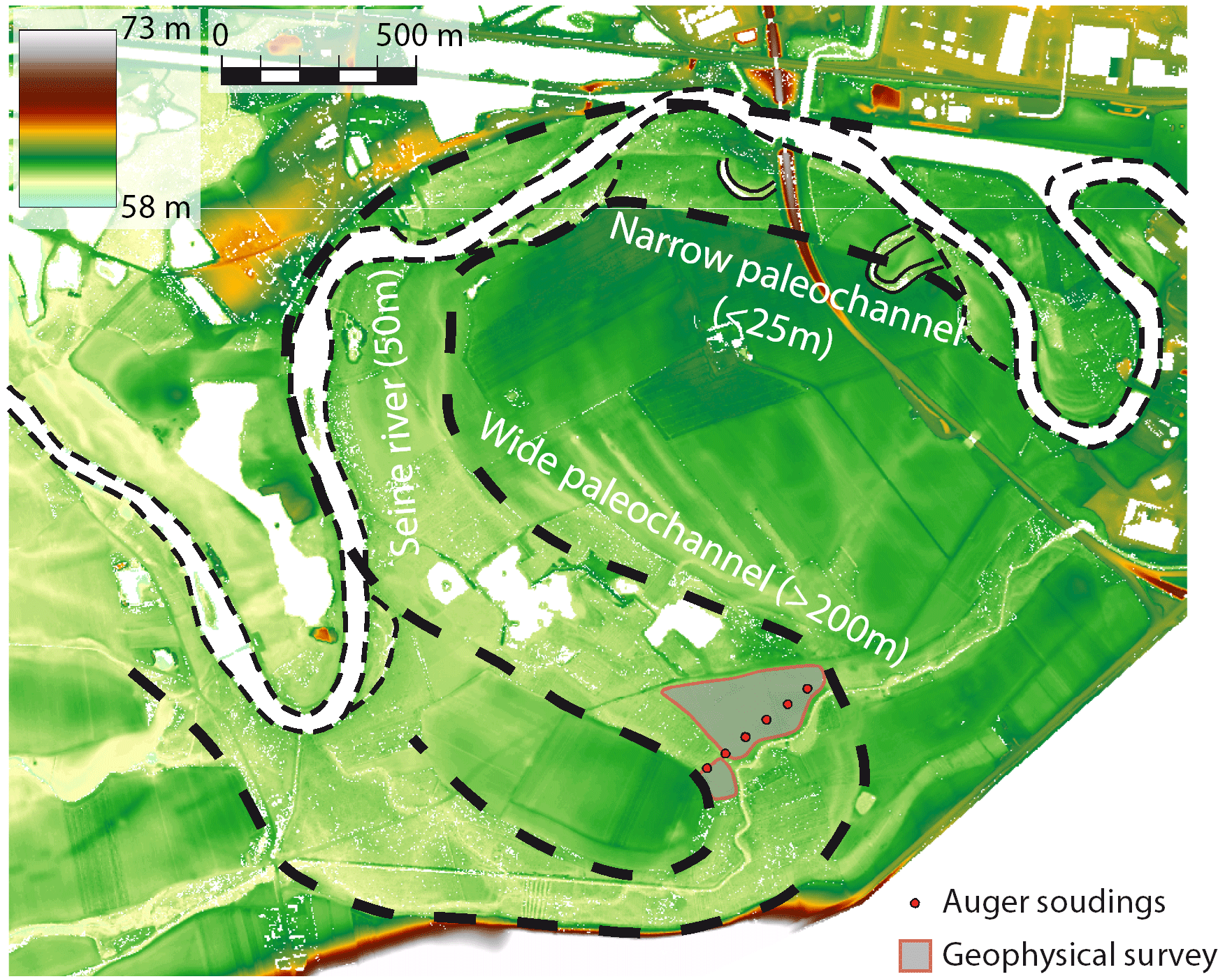
Figure 2Lidar map of the study area, showing the contemporary location of the Seine River, together with the narrow and wide paleochannel interpretations.
Geophysical investigations of gravel pits (after removal of the conductive topsoil) were carried out using ground-penetrating radar (Deleplancque, 2016), and have contributed to the characterization of the sedimentary contrast of the sand bar architecture, between the Weichselian and Holocene deposits. The Weichselian deposits are typical of braided fluvial systems, with fluvial bars of moderate extent (< 50 m) truncated by large erosional surfaces. The thickness of the preserved braid bars rarely exceeds 1.5 m. The Holocene architecture is associated mainly with single-channel meandering fluvial systems, characterized by thick point-bar deposits (> 4 m) with a lateral extent of several hundred metres, sometimes interrupted by clayey paleochannel infillings. Traces of small sinuous channels, probably using the paths of former Weichseilian braided channels, are also identified at the edge of the alluvial plain.
Aerial photography and a lidar (laser detection and ranging) topographic survey (Fig. 2) have been used to characterize the paleochannel plan-view morphologies (style, width, meander wavelength), of the most recent (Holocene) meandering alluvial sheets in this area (Deleplancque, 2016). These measurements were complemented by auger soundings and 14C dating of organic debris or bulk sediment (peat), in order to determine a time frame for the development of the Seine meanders and to allow these changes to be compared with other regional studies (e.g. Antoine et al., 2003; Pastre et al., 2003). The paleochannel investigated in this study is located 2 km to the southwest of Nogent-sur-Seine (covered by a grassy meadow) and is characterized by larger dimensions than the present-day Seine River. Its width is estimated to lie between 150 and 300 m, with a meander wavelength between 2 and 3 km. According to the alluvial sheet analysis and the dating of organic material in the mud plug of the abandoned meander, it is very likely that this paleochannel was active between the Late Glacial and Preoboreal periods (Deleplancque, 2016).
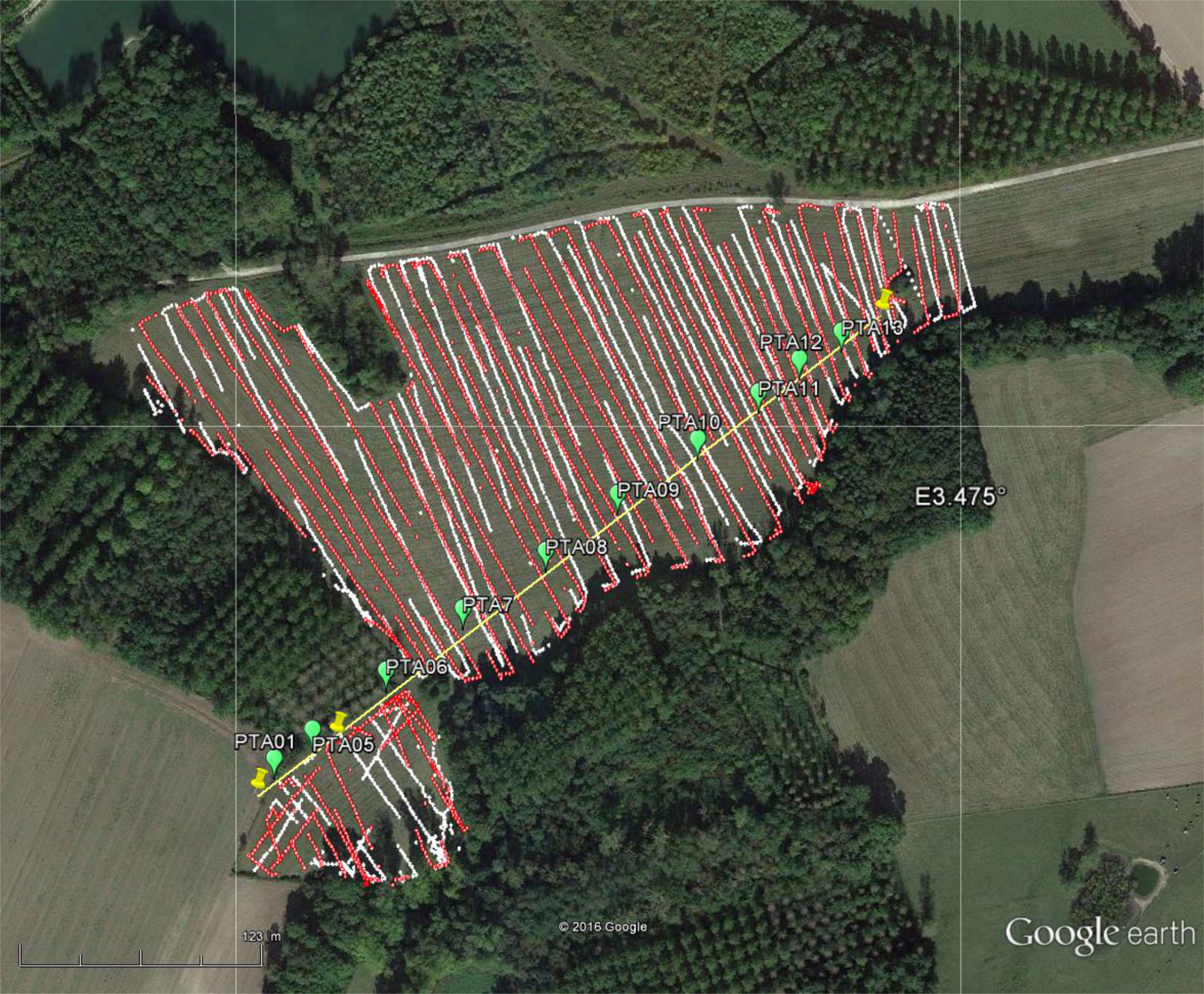
Figure 3Map of the surveyed area, showing the locations of the VCP (red) and HCP (white) measurements (GPS issues explain the holes within the lines). The reference (ERI) profile, recorded with a Wenner–Schlumberger configuration using 1 m electrode spacing between 0 and 350 m, and a 0.5 m electrode spacing between 350 and 401.5 m, is indicated by the yellow line. As green dots, the locations of the hand auger drillings.

Figure 4Log of hand auger soundings performed along the reference profile. The position of each sounding along the ERI profile is shown in Fig. 5.
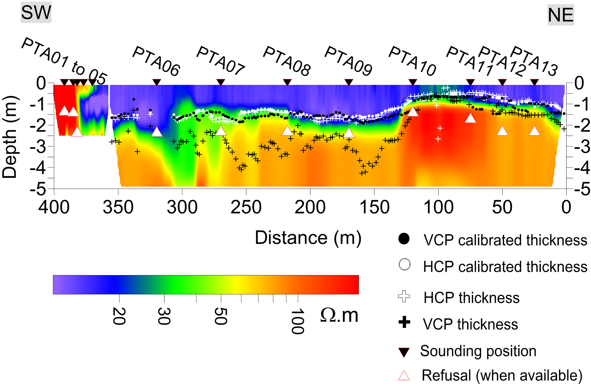
Figure 5Results from the electrical resistivity imaging (ERI) inversion, computed along the reference profile. This section reveals the two main (conductive and resistive) geological units. The markers correspond to the inverted location of the interface (from EMI measurements) between the conductive unit and the substratum, before and after linear calibration (Fig. 6). This figure shows that calibration of the raw VCP measurements leads to significant corrections in inverted depth, when compared to the calibration of the HCP measurements.
The survey coordinates were determined through the use of a lidar map (Deleplancque, 2016), combined with the analysis of a series of auger soundings made along a reference transect of almost 400 m in length (Figs. 2 and 3). The lateral extent of the meander was delineated using an EMI system (CMD explorer) produced by GF Instruments s.r.o., with non-regular gridding and non-perfect overlapping inside the same area.
3.1 ERI and hand auger soundings results
A total of 13 hand auger soundings down to a maximum depth of 2.4 m (Fig. 4) were made along the reference profile. Some of these soundings did not reach the base of the paleomeander mud plug (clay–gravel transition), suggesting that the maximum depth of the paleomeander is greater than 2.4 m. The auger soundings revealed the presence of two main units. The uppermost unit is comprised of topsoil, which overlies a layer of loam containing a significant proportion of gravel and sand in the eastern part of the reference profile. A clayey layer, the bottom of which was not reached in the deepest portion of the paleochannel, is situated below this unit. In some soundings, the clayey facies contains layers of peat (PTA, 04, 05, 06, 08, and 09, in Fig. 4).
The identification of the Holocene clay infilling along this reference profile was confirmed by measuring several and overlapping ERI profiles (24 m common), along the reference transect. For this, a Wenner–Schlumberger array was selected, with 48 electrodes positioned at a 1 m spacing for the first 340 m, and a 0.5 m spacing thereafter.
The ERI cross section (Fig. 5) is produced using a dataset of more than 5000 measurements. A Wenner–Schlumberger reciprocal array was used, which provides a good compromise between lateral and depth sensitivities (Furman et al., 2003; Dahlin and Zhou, 2004). In order to estimate the interpreted resistivity distribution, the resulting apparent resistivity sections were processed by means of inverse numerical modelling using the Res2dinv software (Loke et al., 2003) with its default damping parameters, and the robust (L1-norm) method. Following a total of seven iterations, the resulting ERI profiles had an rms error of 0.48 and 0.93 %, for the case of the 1 and 0.5 m electrode spacings, respectively.
The resistivity cross section reveals two main units: an uppermost conductive unit with a resistivity below 20 Ωm, corresponding to a clayey matrix, and a second, more resistive unit with a resistivity greater than 60 Ωm, associated with a medium/coarse-grained silty horizon. The auger soundings are always achieved by a refusal, which is most likely due to the fact that they had reached the resistive second unit. When compared to the analysis achieved using auger soundings, the electrical properties of the topsoil/loam formation appear to be merged with the clayey formation, with the exception of the western portion of the cross section, which has significant sand and gravel content. This outcome could also be due to the finer spatial resolution of the ERI measurements (electrode spacing of 0.5 m). It is worth noting that the current sensitivity issue associated with the topsoil/loam identification could have probably been overcome with a gradient or a multiple gradient array, without significant loss in DOI (Dahlin and Zhou, 2006).
3.2 EMI surveys and calibration
EMI surveys were carried out using a CMD explorer (GF instruments), at 1 m height above the ground, with vertical (HCP, horizontal co-planar) and horizontal (VCP, vertical co-planar) magnetic dipole configurations. The CMD explorer operates at 10 kHz, and allows simultaneous measurements to be made with three pairs of Tx-Rx coils (unique Tx coil), using a single orientation (T mode). Three different offsets were used between the centres of the Tx and the Rx coils, namely 1.48, 2.82, and 4.49 m, each corresponding to a distinct DOI (approximately 2.2, 4.2, 6.7 m for HCP respectively, and 1.1, 2.1, 3.3 m for VCP respectively). As the VCP and HCP surveys were made separately in continuous mode (0.6 s time step), slightly different sampling intervals were used. In addition, GPS reception difficulties led to several gaps in the VCP and HCP surveys. It was thus important to carefully evaluate these shortcomings, before merging the HCP and VCP datasets prior to the inversion. As the CMD allows the user to export raw out-of-phase data (including the factory calibration only), no pre-processing is needed to obtain the value of the ratio between the secondary and primary magnetic field amplitude.
Apparent electrical conductivities measured using EMI are particularly sensitive to the orientation of the device, the height above the ground at which the EMI system is set up during the survey, and the 3-D variability of the EC. In addition, for the interpretation of the measurements, the ground is assumed to be horizontally layered at any given location, even for the smallest dipole offset. It is worth noting that even if the orientation (vertical or horizontal) and height of the dipole are initialized at the beginning of each survey, variations of orientation and height of the EMI device inevitably occur and add noise to the measurements.
In order to improve absolute (not relative) evaluation of EMI data, in situ calibration of EMI data is important. Ideally, calibration must be performed for several heights and over a perfectly known half-space of which electromagnetic properties span over a representative range of ECa values. For the CMD instrument, calibration factors are provided by the manufacturer for 0 (laid on ground) and 1 m heights. However, those factors are valid for a given ECa range and are dependent on the prospection height (which is never exactly 1 m). This height effect, as mentioned above, has a relatively stronger influence on the shortest offsets; consequently, to improve the absolute estimation of ECa, it is important to have a reference zone where the ground is very well constrained. In order to obtain deeper information than obtained with the hand-made auger soundings, an ERI prospection has been carried out; the inversed ERI section provides reference and absolute values of the local resistivities and can be used in the calibration process as described in Lavoué et al. (2010). It is worth noting that other in situ ways of calibration could be performed (e.g. Delefortrie et al., 2014) – particularly, using the theoretical response of a metallic and non-magnetic sphere (Thiesson et al., 2014).
During the field data acquisition we faced several difficulties that prevented us from taking a CMD profile exactly on the reference profile. Actually, the EMI data used for the calibration have been taken from the mapped data closest to the reference profile. This led to several positioning and alignment errors because: (1) the EMI data do not exactly cross the reference profile, (2) the EMI data are irregularly spaced along the ERI profile, (3) the orientation of the CMD device was not exactly the same for each measurement retained for the calibration, and (4) the height above the surface is changing constantly during the acquisition (less than 10–20 cm).
In order to compute the ECa of a layered ground, based on measurements made using a horizontal or vertical magnetic dipole configuration, we used the well-known electromagnetic analytical solution for cylindrical model symmetry (given by Wannamaker et al. 1984; Ward and Hohmann, 1988; Xiong, 1989). However, in the case of thin layers or high-frequency content, convergence problems can be encountered in the numerical integration of the corresponding oscillating Bessel functions. At frequencies below 100 kHz, as in the case of the present study, the numerical filters developed by Guptarsarma and Singh (1997) were found to provide an efficient solution to this problem. The inversion scheme developed by Schamper et al. (2012) was used to invert the EMI measurements. For each offset and dipole orientation, a linear relationship (shifting and scaling) is determined between each measured ECa and the ECa estimated from the resistivity models (derived from the ERI panel, Fig. 6). Once the calibration has been done, the new EMI inversion matches the ERI used for the calibration, which illustrates the validity of the procedure. Despite the linear relationship assessed between the EMI and ERI resistivities, several non-linear operations are applied: (1) ERI local 1-D models along the profile are used to simulate EMI measurements, (2) EMI field data are then fitted (linearly) to those simulations using a non-linear optimization procedure to estimate calibration factors, and (3) finally the calibrated/shifted data are inverted with a non-linear forward modelling. Each of the previous operations implies a necessary check to ensure that the calibration process has been correctly applied. Step (3) does not guarantee that estimated interfaces will match the ERT interfaces (1) if the fixed/chosen resistivities are not correct, or (2) if EMI does not integrate the ground in the same way as the ERI in the case of strong anisotropy. This does not seem to be the case here, since a good match is obtained.
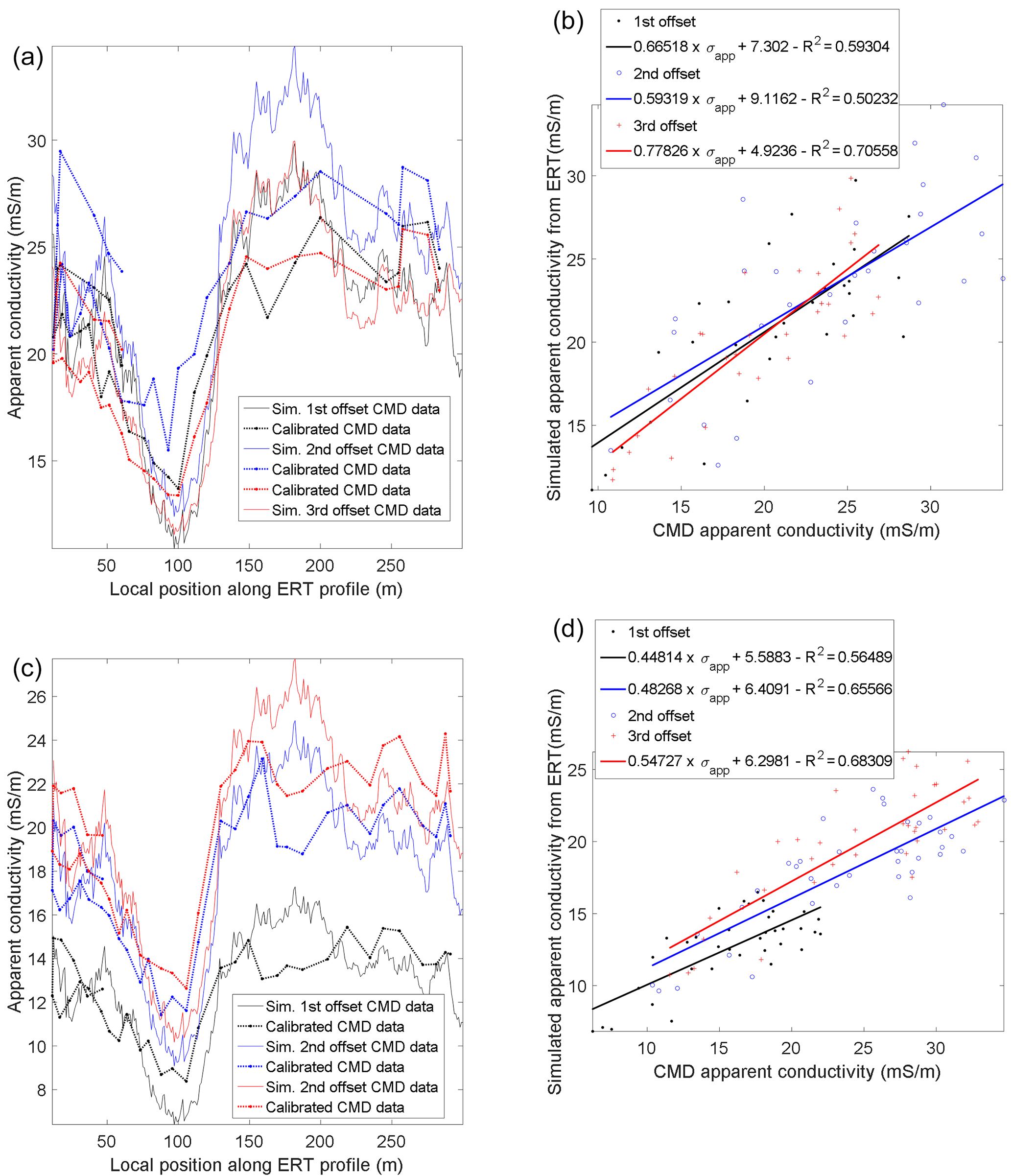
Figure 6HCP (a) and VCP (c) calibration results obtained along the reference profile: simulated apparent CMD conductivities based on the ERI inversion compared to the calibrated EMI measurements. Scatter plots of the HCP (b) and VCP (d) measured vs. simulated apparent conductivities. The solid lines indicate the corresponding linear regressions.
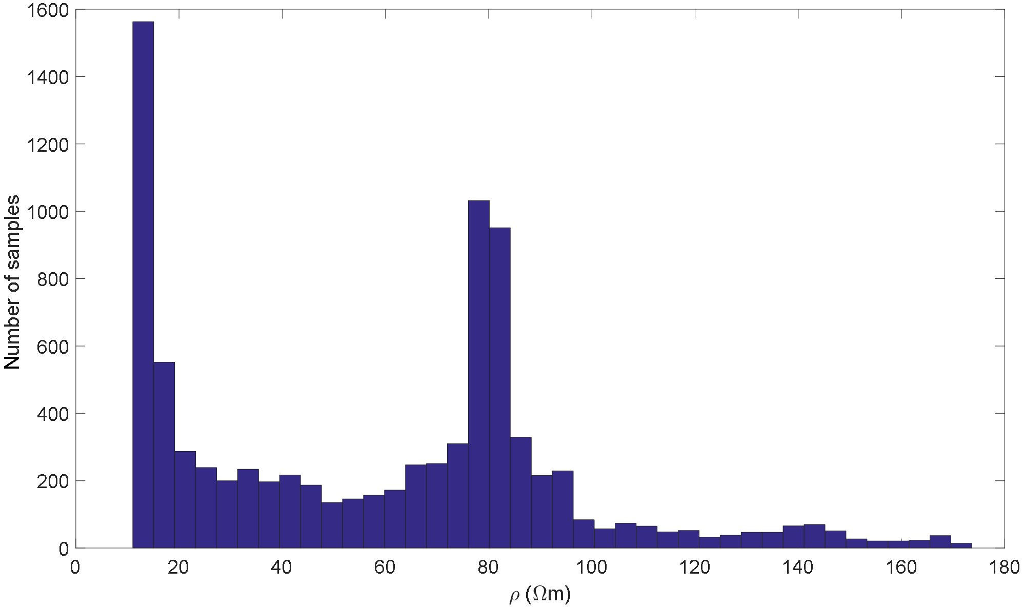
Figure 7Histogram of the electrical resistivity values determined for the ERI section shown in Fig. 5.
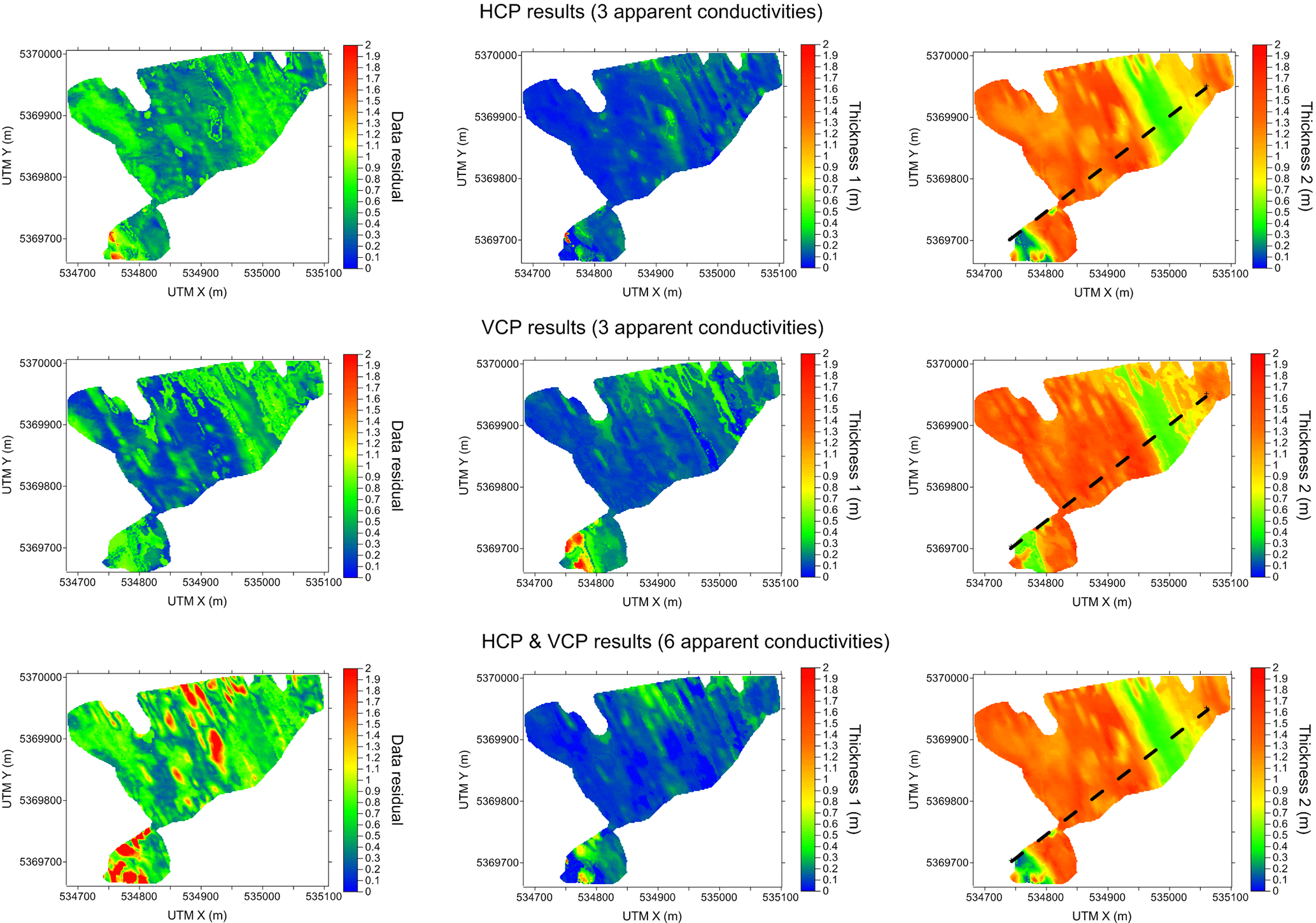
Figure 8Results of the CMD inversion, including the data residual (left column), for a three-layer model (1: topsoil; 2: conductive filling; and 3: resistive substratum). The thicknesses 1 and 2 correspond to the topsoil and conductive filling, respectively. The prospection height is 1 m. The conductivities are set to σ1= 13 mS m−1, σ2= 72 mS m−1 and σ3= 13 mS m−1. A noise level of 1 mS m−1 on the apparent conductivities was assumed, with a minimum relative error of 5 %. The black dashed line indicates the ERI reference profile location.
The correlation coefficients range between 0.5 and 0.7. Such values can be explained by several sources of errors in the estimation of the EMI apparent conductivities along the reference profile: (1) the differences in the location between the EMI measurements used for the calibration and the ERI profile, (2) the fact that the 1-D model used for the EMI modelling is extracted from the inversed 2-D resistivity section, and (3) the difference of sensitivity between the ERI and EMI data. The regressions indicate the need of a stronger correction for the VCP configuration than for the HCP configuration. The scaling correction decreases as a function of offset, particularly for the HCP, which can be explained by the fact that small offsets are more sensitive to positioning and orientation errors, as well as to natural near-surface variabilities.
3.3 EMI inversion parameters
Once the calibration process is completed, the corrected, apparent HCP and VCP conductivities are inverted, following their interpolation (by kriging) onto the same regular grid. The ERI results indicate a two-layer model (but do not highlight the topsoil), while the auger soundings show a topsoil layer of a few decimetres thickness above the conductive formation. Consequently, a three-layer model seems reasonably justified all over the site during the inversion process to represent the studied area: a resistive topsoil, a conductive clayey filling, and a resistive sand/gravel layer. The resistivity of each layer corresponds to the peak values of the bimodal histograms of the reference 1 m spaced ERI profile, as shown in Fig. 7. The topsoil EC derived from the half-metre-spaced ERI profile in the western portion is found to be very similar to the EC of the resistive layer inferred from the 1 m spaced ERI profile – thus, the first and third layer EC are considered to be equal. This leads to the following model for the mean EC of the three layers: σ1= 13 mS m−1; σ2= 72 mS m−1; σ3= 13 mS m−1. It should be noted that the CMD explorer is operated at a single frequency (10 kHz). The sounding height was taken to be 1 m for all the field measurements.
It is worth noting that the three-layer model chosen instead of a two-layer model, all over the site, might be questionable. Letting the inversion process decide between a three- or two-layer model could have been an option. In the present case, the difference between a two-layer or three-layer model is clearly negligible where the interpreted thickness of the topsoil (for the three-layer model) is less than a few decimetres. For such low thicknesses the topsoil can be considered as non-existent considering the acquisition geometry and settings of the CMD explorer.
Figure 8 shows the inverted thicknesses of the first and second layers, and the data residual for the HCP (three offsets), the VCP (three offsets), and the combined HCP and VCP conductivities (six apparent values). The standardized root-mean-squared residual (SRMR) for N independent measurements is given by
where N is the number of data points, d is the forward response of the estimated model at the end of the inversion, dmeas contains the data, and SD is the standard deviation of the data. The standard deviation (SD) was estimated from repeated measurements at several locations, as 1 mS m−1 (with a minimum error of 5 %).
3.4 EMI results
3.4.1 General trend
The layer thickness inversion was performed using three different datasets: (1) the HCP dataset, (2) the VCP dataset, and (3) the combined HCP and VCP dataset (Fig. 8).
Whatever the dataset used for the inversion, the thickness computed for the topsoil formation (indicated by “Thickness 1” in Fig. 8) is globally very small (blue), whereas that computed for the conductive infilling (indicated by “Thickness 2”) has a significantly higher value (red), and vice versa. Although it varies in thickness, the conductive layer formation spans most of the survey area, whereas the resistive topsoil formation varies mainly in two distinct locations: (1) the southwestern limit of the surveyed area, where it reaches a depth of 2 m, and (2) the mid-northern portion of the surveyed area, where its thickness never exceeds 0.6 m. In addition, very small scale topsoil formations are scattered over the surveyed area. In all places where the estimated thickness of the first layer is less than 20 cm, the topsoil can be considered as inexistent and a two-layered model is enough to explain EMI data. Nevertheless, all of the observed topsoil formations appear to be correlated with a local increase in data residual. The thickness of the conductive infilling lying below the topsoil formation ranges between 0 m, in the southwestern portion of the studied zone, and its maximum value of almost 2 m at the centre of the map.
The VCP mode increases the measured thickness of the shallowest portions of the topsoil layer, whereas the HCP mode tends to negate this layer over most of the surveyed area (central part), where it is not extremely thick. This tendency appears to be correlated with a slight increase in the thickness of the second conductive layer.
The inversion of all data, in the form of a single dataset, appears to lead to a mixture of the properties inherent to each of the constituent datasets. This outcome is particularly noticeable in the case of the topsoil formation, where certain structures retrieved by both datasets are emphasized with respect to structures that are present in only one or the other of these.
3.4.2 Internal variability
In addition to strong meander wavelength variations, each dipole orientation reveals different level of heterogeneities in the material present in the conductive infilling, as well as the topsoil. Concerning the material close to the surface (< 2 m), this variability is clearly illustrated by the auger soundings, whereas the conductive unit identified by the ERI section is considerably more complex. In simple terms, the thickness of the conductive material tends to decrease, wherever the silty and sandy material reaches the surface.
It should be noted that the inversions observed for each dipole orientation are not systematically preserved in the inversion produced by combining the data from both dipole orientations. This result indicates that in the present context, each orientation is complementary, and contributes a specific set of information. This is particularly relevant in the northern portion of the studied area, where the thickness of the first resistive layer is more variable when it is measured with the horizontal dipole configuration (VCP) than with the HCP configuration.
The data residual has numerous peaks in the southwestern portion of the study zone. In this zone, the resistive topsoil reaches a thickness of 1 m, leading to EMI measurements with a lower sensitivity (and thus lower signal-to-noise ratio, SNR). The combined HCP and VCP data inversion naturally leads to the occurrence of higher values of data residual than in the case of the individual HCP or VCP inversions. Indeed, it is difficult to compare the data residual maps between the three proposed datasets (i.e. HCP alone, VCP alone, and both) as the physical contribution associated with each dataset inversion result is related to the coupled dataset–model used for the inversion. HCP and VCP modes do not integrate the ground in the same way exactly. If the ground within the footprint of the EMI system is a bit far from a tabular model, then the interpretation with local 1-D models can be more difficult with both datasets combined than with only one of the two sets analysed. The difficulty to invert the HCP and VCP datasets jointly also arises because (1) the locations of the soundings between the two surveys are not exactly the same as the modes cannot be acquired at the same time, (2) the heights varies differently, and (3) the pitch and roll are not constant. For those last two points one could imagine the monitoring of these “flight” parameters to correct the data, which is routinely done for airborne electromagnetic surveys. But this feature does not exist at the present time for ground-based EMI devices.
In the present study, the outcomes of ERI and EMI surveys integrate quite satisfactorily the lithological information provided by the auger soundings, but have not yet been checked with exhaustive hydrological information. During the presented geophysical campaign (low-water period), the water level measured from PTA02 to PTA04 and from PTA11 to PTA13 locations indicate a groundwater situated at 1 m depth, roughly at the interface between the clay infilling and the upper geological unit (Fig. 4). In the survey area the water table could rise close to the surface at high-water periods, which implies that the conductivity of the topsoil/loam formation should increase. In the closest piezometer located 1 km west from the prospected site, the water table was situated at 70 cm below the surface. The EC measured in the same piezometer in 2011 was 640 µS cm−1 (15.6 Ωm) and showed a seasonal variation of the water table of approximately 60 cm (Voies Naviguables de France (VNF) Technical Report, 2011).
The clay infilling is thus always saturated while the topsoil/loam upper unit is almost never dry. Even significant changes in the degree of saturation of the topsoil/loam formation would hardly allow the value of its resistivity to fall to the resistivity of the clay infilling (∼ 10–20 Ωm) estimated from the histogram (Fig. 7). Consequently, if the thickness of the topsoil/loam formation is significantly larger than a few decimetres, the presence of the water table at the surface does not challenge the three-layer model assumption based on the lithological boundaries.
From a hydrogeological modelling perspective, one of the most important issues is the assessment of the constitutive relationship that links EMI/ERI electrical conductivity/resistivity to hydrodynamic properties (i.e. the permeability) because of the difficulty in discriminating the bulk conduction from the surface conduction mechanism. In the present case, a sample located at PTA12 and at a depth between 140 and 160 cm shows major peaks of calcite and quartz, significant peaks of illite-montmorillonite, and small peaks of kaolinite. The clayey infilling corresponds to a saturated marl sediment containing 20–30 % of clay and 50–60 % carbonate. The high amount of carbonate originates from the weathering of the chalky cretaceous limestones that outcrop on the borders of the alluvial plain. As the salinity is low and the clay content significant, the electrical conductivity of the clayey infilling is essentially driven far more by the surface conductivity than by the pore water conductivity. As this is not the case for the first decimetre of topsoil/loam, it could be another argument that reinforces the pertinence of the three-layer model assumption for the inversion process.
From a more general perspective, EMI calibrated with ERI and auger soundings contributed to a better characterization of the geometry and variability of this paleomeander. The results reveal a complex cross-sectional geometry of the conductive clayey layer, featuring from the southwest to the northeast: (1) a sharp contact to the southwest with a resistive sand and gravel layer, (2) a roughly constant thickness of 2 m of the conductive layer, extending over more than 200 m, (3) a decrease in the thickness of the conductive layer (∼ 0.5 m) related to the raising of the gravely substrate, over a length of ∼ 100 m, and (4) an increase in the thickness of the conductive layer to the northeast. Unfortunately, the contact of the conductive layer with the resistive layer to the northeast was not captured, due to the limited extent of the surveyed area. It is thus difficult to conclude whether the paleomeander is restricted between PTA03 and PTA10, with a mean depth of 2 m and a width of 250 m, or whether the former channel was wider (> 350 m) with a shallower part associated with sand/gravel bars. It is also not excluded that several (2 or 3) small channels were active during low-water stages within a larger “bankfull channel”, producing local incision of the bed. Nevertheless, and compared to the modern Seine River (∼ 50 m wide, up to 5 m deep), this paleochannel attributed to the Late Glacial/Preboreal period shows a larger width, and a significantly larger width-to-depth ratio. These differences are attributed to different paleohydrological and paleoclimatic conditions, with larger water discharges, larger and coarser solid fluxes, and less cohesive soils in the absence of developed vegetation.
From a hydrogeological perspective, the paleomeanders of the Late Glacial/Preboreal period are filled with large but relatively thin (2 m) mud plugs compared to the alluvial plain thickness (6 to 8 m), which should produce little impact on the groundwater flow. However, this should be confirmed by numerical modelling. The study should be extended to paleomeanders attributed to different climatic periods of the Holocene, which present different morphologies and aspect ratios.
We presented the results of the geophysical investigations of a paleochannel in the Bassée alluvial plain (Seine Basin, France). The location of this paleochannel and its geometry, suggested by a lidar campaign, have been accurately mapped using a multi-configuration (various offsets and orientations) electromagnetic induction device.
In order to correct the drift and factory calibration issues arising from EMI measurements, a calibration procedure was implemented, based on the use of a linear correction with ERI inversion results and auger soundings. The shifting and scaling of EMI HCP and VCP measurements was made for the three available offsets (1.48, 2.82, and 4.49 m), at a frequency of 10 kHz. Six apparent conductivities allowed the inversion of a reliable three-layer model, comprising a conductive filling with an EC equal to 72 mS m−1 below the topsoil, and a resistive substratum having an EC equal to 13 mS m−1. The conductivities of the three-layer model were adjusted using the bimodal histogram distribution of the reference ERI profile. The inverted thicknesses are characterized by a significant internal variability in the conductive filling and the topsoil, associated with the paleochannel geometry.
The joint inversion of multi-offset HCP and VCP configurations leads to a very interesting result, in which the internal variability description is considerably enhanced. We believe that multi-configuration EMI geophysical survey carried out at an intermediate scale should provide a great complement to TDR (time domain reflectometry) for a quantitative and physical calibration of remote sensing soil properties and moisture content. Combined multi-offset VCP and HCP prospections could significantly improve the accuracy of hydrogeological modelling by potentially providing a hydrogeological picture of the first metres sedimentary setting in terms of lithological distribution; but it would also lead to a substantial increase in survey costs with the instruments currently available on the market.
In order to access the data, we ask researchers to contact the corresponding author (faycal.rejiba@univ-rouen.fr).
The authors declare that they have no conflict of interest.
This research was supported by the PIREN Seine research programme (2015–2019).
We extend our warm thanks to Christelle Sanchez for her participation in the
geophysical survey and to Laurence LeCallonnec for carrying out the XRD
experiment.
Edited by: Mauro Giudici
Reviewed by: Bradley Weymer and two anonymous referees
Antoine, P., Coutard, J.-P., Gibbard, P., Hallegouet, B., Lautridou, J.-P., and Ozouf, J.-C.: The Pleistocene rivers of the English Channel region, J. Quaternary Sci., 18, 227–243, 2003.
Benech, C., Lombard, P., Rejiba, F., and Tabbagh, A: Demonstrating the contribution of dielectric permittivity to the in-phase EMI response of soils: example of an archaeological site in Bahrain, Near Surf. Geophys., 14, 337–344, 2016.
Berger, G., Delpont, G., Dutartre, P., and Desprats, J.-F.: Evolution de l'environnement paysager de la vallée de la Seine – Cartographie historique et prospectives des explorations alluvionnaires de la Bassée, French Geological Survey (BRGM) report R 38 726, 39 pp., 1995.
Caillol, M., Camart, R., and Frey, C.: Synthèse bibliographique sur la géologie, l'hyrogéologie et les ressources en matériaux de la région de Nogent-sur-Seine (Aube), French Geological Survey (BRGM) report 77 SGN 303 BDP, 108 pp., 1977.
Dahlin, T. and Zhou, B.: A numerical comparison of 2-D resistivity imaging with 10 electrode arrays, Geophys. Prospect., 52, 379–398, 2004.
Dahlin, T. and Zhou, B.:Multiple-gradient array measurements for multichannel 2-D resistivity imaging, Near Surf. Geophys., 4, 113–123, 2006.
Delefortrie, S., De Smedt, P., Saey, T., Van De Vijver, E., and Van Meirvenne, M.: An efficient calibration procedure for correction of drift in EMI survey data, J. Appl. Geophys., 110, 115–125, 2014.
Deleplancque, B. : Caractérisation des hétérogénéités sédimentaires d'une plaine alluviale: Exemple de l'évolution de la Seine supérieure depuis le dernier maximum glaciaire, PhD Thesis, PSL Research University, Paris, France, 273 pp., 2016.
De Smedt, P., Van Meirvenne, M., Meerschman, E., Saey, T., Bats, M., Court-Picon, M., De Reu, J., Zwertvaegher, A., Antrop, M., Bourgeois, J., and De Maeyer, P.: Reconstructing palaeochannel morphology with a mobile multicoil electromagnetic induction sensor, Geomorphology, 130, 136–141, 2011.
Everett, M. E.: Theoretical developments in electromagnetic induction geophysics with selected applications in the near surface, Surv. Geophys., 33, 29–63, 2012.
Fitterman, D. V., Menges, C. M., Al Kamali, A. M., and Jama, F. E.: Electromagnetic mapping of buried paleochannels in eastern Abu Dhabi Emirate, UAE, Geoexploration, 27, 111–133, 1991.
Flipo, N., Mouhri, A., Labarthe, B., Biancamaria, S., Rivière, A., and Weill, P.: Continental hydrosystem modelling: the concept of nested stream–aquifer interfaces, Hydrol. Earth Syst. Sci., 18, 3121–3149, https://doi.org/10.5194/hess-18-3121-2014, 2014.
Friedman, S. P.: Soil properties influencing apparent electrical conductivity: a review, Comput. Electron. Agr., 46, 45–70, 2005.
Furman, A., Ferré, T., and Warrick, A. W.: A sensitivity analysis of electrical resistivity tomography array types using analytical element modeling, Vadose Zone J., 2, 416–423, 2003.
Guptasarma, D. and Singh, B.: New digital linear filters for Hankel J0 and J1 transforms, Geophys. Prospect., 45, 745–762, 1997.
Jordan, D. W. and Prior, W. A.: Hierarchical Levels of Heterogeneity in a Mississippi River Meander Belt and Application to Reservoir Systems: Geologic Note, AAPG Bulletin, 76, 1601–1624, 1992.
Huang, H.: Depth of investigation for small broadband electromagnetic sensors, Geophysics, 70, G135–G142, 2005.
Lavoué, F., Van Der Kruk, J., Rings, J., André, F., Moghadas, D., Huisman, J. A., Lambot, S, Weihermüller, L., Vanderborght, J., and Vereecken, H.: Electromagnetic induction calibration using apparent electrical conductivity modelling based on electrical resistivity tomography, Near Surf. Geophys., 8, 553–561, 2010.
Loke, M. H., Acworth, I., and Dahlin, T.: A comparison of smooth and blocky inversion methods in 2-D electrical imaging surveys, Explor. Geophys., 34, 182–187, 2003.
McNeill, J. D.: Electromagnetic terrain conductivity measurement at low induction numbers, Geonics Technical Note TN-6, 1980.
Mégnien, F. : Possibilités aquifères des alluvions du val de Seine entre Nogent-sur-Seine et Montereau, incluant la carte géologique et géomorphologique de la Bassée, French Geological Survey (BRGM) report 65-DSGR-A-076, 452 pp., 1965.
Miall, A. D.: Reservoir Heterogeneities in Fluvial Sandstones: Lessons from Outcrop Studies, AAPG Bulletin, 72, 682–697, 1988.
Mordant, D. : La Bassée avant l'histoire : archéologie et gravières en Petite-Seine, Association pour la promotion de la recherche archéologique en Ile-de-France, Nemours, 143 pp., 1992.
Nabighian, M. N.: Electromagnetic methods in applied geophysics (Vol. 1), SEG Books, 1988a.
Nabighian, M. N.: Electromagnetic methods in applied geophysics (Vol. 2), SEG Books, 1988b.
Pastre, J.-F., Limondin-Lozouet, N., Leroyer, C., Ponel, P., and Fontugne, M.: River system evolution and environmental changes during the Lateglacial in the Paris Basin (France), Quaternary Sci. Rev., 22, 2177–2188, 2003.
Rhoades, J. D., Raats, P. A. C., and Prather, R. J.: Effects of liquid-phase electrical conductivity, water content, and surface conductivity on bulk soil electrical conductivity, Soil Sci. Soc. Am. J., 40, 651–655, 1976.
Schamper, C., Rejiba, F., and Guérin, R.: 1-D single-site and laterally constrained inversion of multifrequency and multicomponent ground-based electromagnetic induction data – Application to the investigation of a near-surface clayey overburden, Geophysics, 77, WB19–WB35, 2012.
Simon, F. X., Sarris, A., Thiesson, J., and Tabbagh, A.: Mapping of quadrature magnetic susceptibility/magnetic viscosity of soils by using multi-frequency EMI, J. Appl. Geophys., 120, 36–47, 2015.
Spies, B. R.: Depth of investigation in electromagnetic sounding methods, Geophysics, 54, 872–888, 1989.
Tabbagh, A.: Applications and advantages of the Slingram electromagnetic method for archaeological prospecting, Geophysics, 51, 576–584, 1986.
Thiesson, J., Kessouri, P., Schamper, C., and Tabbagh, A.: About calibration of frequency domain electromagnetic devices used in near surface surveying, Near Surf. Geophys., 12, 481–491, 2014.
VNF (Voies navigables de France): Etat des lieux de la piézométrie de la petite Seine, Technical Report, 58 pp., 2011 (in french).
Wannamaker, P. E., Hohmann, G. W., and Sanfilipo, W. A.: Electromagnetic modeling of three-dimensional bodies in layered earths using integral equations, Geophysics, 49, 60–74, https://doi.org/10.1190/1.1441562, 1984.
Ward, S. H. and Hohmann, G. W.: Electromagnetic theory for geophysical applications, in: Electromagnetic methods in applied geophysics, Vol. 1: Theory, edited by: Nabighian, M. N., 131–311, 1988.
Xiong, Z.: Electromagnetic fields of electric dipoles embedded in a stratified anisotropic earth, Geophysics, 54, 1643–1646, https://doi.org/10.1190/1.1442633, 1989.