the Creative Commons Attribution 3.0 License.
the Creative Commons Attribution 3.0 License.
On the use of the GRACE normal equation of inter-satellite tracking data for estimation of soil moisture and groundwater in Australia
Natthachet Tangdamrongsub
Shin-Chan Han
Mark Decker
In-Young Yeo
Hyungjun Kim
An accurate estimation of soil moisture and groundwater is essential for monitoring the availability of water supply in domestic and agricultural sectors. In order to improve the water storage estimates, previous studies assimilated terrestrial water storage variation (ΔTWS) derived from the Gravity Recovery and Climate Experiment (GRACE) into land surface models (LSMs). However, the GRACE-derived ΔTWS was generally computed from the high-level products (e.g. time-variable gravity fields, i.e. level 2, and land grid from the level 3 product). The gridded data products are subjected to several drawbacks such as signal attenuation and/or distortion caused by a posteriori filters and a lack of error covariance information. The post-processing of GRACE data might lead to the undesired alteration of the signal and its statistical property. This study uses the GRACE least-squares normal equation data to exploit the GRACE information rigorously and negate these limitations. Our approach combines GRACE's least-squares normal equation (obtained from ITSG-Grace2016 product) with the results from the Community Atmosphere Biosphere Land Exchange (CABLE) model to improve soil moisture and groundwater estimates. This study demonstrates, for the first time, an importance of using the GRACE raw data. The GRACE-combined (GC) approach is developed for optimal least-squares combination and the approach is applied to estimate the soil moisture and groundwater over 10 Australian river basins. The results are validated against the satellite soil moisture observation and the in situ groundwater data. Comparing to CABLE, we demonstrate the GC approach delivers evident improvement of water storage estimates, consistently from all basins, yielding better agreement on seasonal and inter-annual timescales. Significant improvement is found in groundwater storage while marginal improvement is observed in surface soil moisture estimates.


The changes in terrestrial water storage (ΔTWS) derived from the Gravity Recovery And Climate Experiment (GRACE) data products have been used in the last decade to study global water resources, including groundwater depletion in India and the Middle East (Rodell et al., 2009; Voss et al., 2013), water storage accumulation in Canada (Lambert et al., 2013), and flood-influenced water storage fluctuation in Cambodia (Tangdamrongsub et al., 2016). The gravity data obtained from GRACE satellites are commonly processed and released in three different product levels (L) that increase in the amount of processing, L1B – satellite tracking data (e.g. Wu et al., 2006), L2 – global gravitational Stokes coefficients (e.g. Bettadpur, 2012), and L3 – global grids (e.g. Landerer and Swenson, 2012). The original (L1B) GRACE information is inevitably altered due to data processing and successive post-processing filterings, because the error covariance information is not propagated through each post-processing step.
The GRACE-derived ΔTWS has been computed widely from the higher-level products (e.g. L2 and L3) on which various ad hoc post-processing filters were applied (e.g. Gaussian smoothing filter, Jekeli, 1981; destripe filter, Swenson and Wahr, 2006). ΔTWS obtained from these filters lacks proper error covariance information and is attenuated and distorted. To overcome the signal attenuation in GRACE high-level products, empirical approaches have been developed, including the application of scale factors computed from land surface models (LSMs; Landerer and Swenson, 2012) to the GRACE L3 products. GRACE uncertainty in the high-level product is usually unknown or assumed. For example, Zaitchik et al. (2008) derived empirically a global average uncertainty that is variable depending on choices of post-processing filters (Sakumura et al., 2014). Furthermore, GRACE error and sensitivity is dependent on latitudes due to the orbit convergence toward poles (Wahr et al., 2006) and any post-processing filters will alter the GRACE data and their error information. Rigorous statistical error information is of equal importance to derivation of ΔTWS for data assimilation and model calibration (Tangdamrongsub et al., 2017; Schumacher et al., 2016, 2018). ΔTWS and its uncertainty estimates should be formulated directly from L1B data considering the complete statistical information.
The GRACE information is not fully exploited in many studies. For example, groundwater storage variation (ΔGWS) is often computed by subtracting the soil moisture variation (ΔSM) component simulated by the land surface model from GRACE-derived ΔTWS data (Rodell et al., 2009; Famiglietti et al., 2011), assuming the model ΔSM is error-free. This may result in the inaccurate ΔGWS and the associated error estimate as the uncertainties in observation and of the land surface model outputs are neglected in the combination (or regression) of two noisy data (e.g. Long et al., 2016). In data assimilation, the GRACE uncertainty is often derived empirically, not necessarily reflecting the actual GRACE error characteristics (e.g. Zaitchik et al., 2008; Tangdamrongsub et al., 2015; Tian et al., 2017). For example, Girotto et al. (2016) used the L3 product and showed that it was necessary to adjust GRACE observation and its uncertainty in order to make their water storage estimates more accurate. Similarly, Tian et al. (2017) reported the need for the application of a scale factor to GRACE uncertainty (from mascon, mass concentration, product) in their GRACE assimilation process. It is apparent that the use of post-processed GRACE products often requires data tuning, leading possibly to an integration of the altered gravity information into the data assimilation system. Some recent studies began to employ the full variance–covariance information in the data assimilation scheme to enhance the quality of the estimates (Eicker et al., 2014; Schumacher et al., 2016; Tangdamrongsub et al., 2017; Khaki et al., 2017a, b).
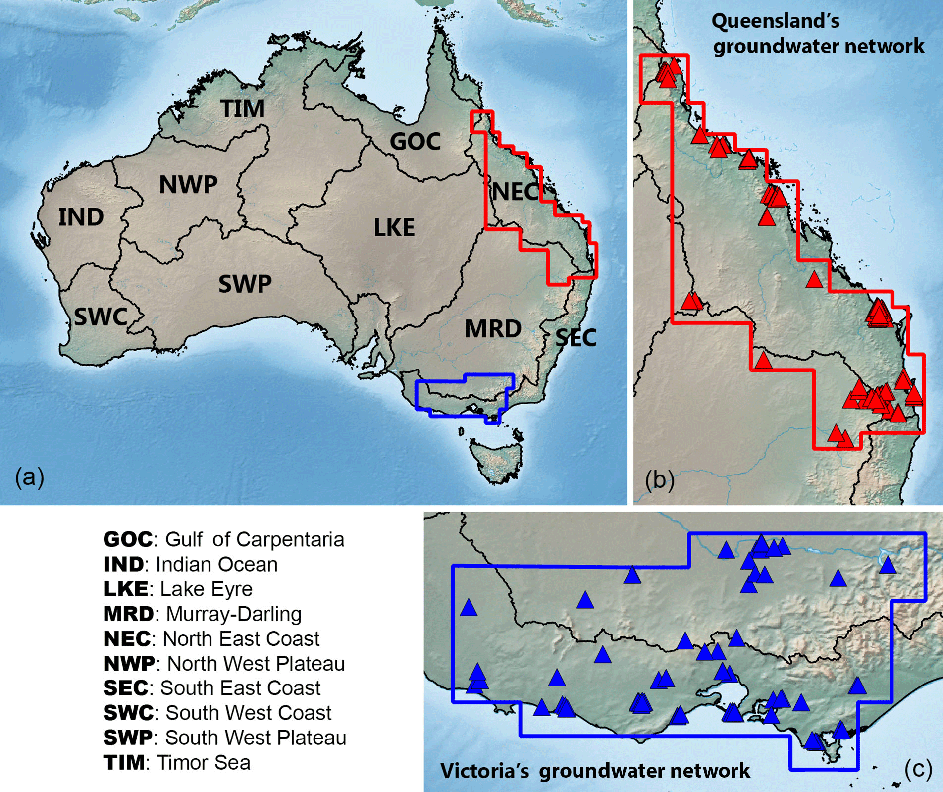
Figure 1(a) Geographical location of 10 Australian river basins. Red and blue polygons indicate the boundaries of the groundwater networks in Queensland (b) and Victoria (c), respectively. Triangles (in b and c) represent the selected bore locations used in this study.
This study aims to use the GRACE information of ΔTWS measurement directly from the least-squares normal equation data. The approach optimally combines GRACE's normal equations with the model simulation results from the Community Atmosphere Biosphere Land Exchange (CABLE, Decker, 2015) to improve ΔSM and ΔGWS estimates. The proposed approach presents three main advantages. Firstly, one can exploit the full GRACE signal and error information by using the normal equation data sets. Secondly, the approach is developed for optimal least-squares combination (e.g. Ramillien et al., 2004), which maximizes the model and observation strength while simultaneously suppressing their weaknesses. Finally, the method bypasses empirical, multiple-step post-processing filters.
The main objective of this study is to present the GRACE-combined (GC) approach to improve the model-estimated ΔSM and ΔGWS on regional scales. We demonstrate our approach applied to 10 Australian river basins (Fig. 1a). One advantage of the study area is that the state vector can be simply defined by ΔSM and ΔGWS as other hydrological components (e.g. snow, glacier) are negligible. We validate the top layer of ΔSM estimates against the satellite soil moisture observation (the Advanced Microwave Scanning Radiometer aboard the Earth Observing System (EOS) – AMSR-E, Njoku et al., 2003) over all 10 basins and the ΔGWS estimates against the in situ groundwater data available over Queensland and Victoria (Fig. 1b and c).
This paper is outlined as follows: firstly, the derivation of the GC approach is presented in Sect. 2 while the description of GRACE data processing, including the use of the GRACE normal equation, is given in Sect. 3. Secondly, the CABLE modelling is outlined in Sect. 4. This includes the derivation of model uncertainty based on the quality of precipitation data and the model parameter inputs. The processing of validation data is also described in Sect. 4. Thirdly, Sect. 5 presents the result of ΔSM and ΔGWS estimates and comparison to in situ data. The long-term trends in the Australian mass variation over the last 13 years are also investigated in this section.
The statistical information of ΔTWS computed from a land surface model can be written as
where h is the “truth” (unknown) model state vector while is the calculated state vector characterized with the model error ϵ. The model error is assumed to have zero mean and covariance C.
The term h is used to represent a vector including the global ΔTWS grid, and terms with a subscript “R” (e.g. hR, CR) are used to represent only a regional set of ΔTWS (for example, in Australia). As such, the observation equation over a region can be rewritten as
As soil moisture and groundwater are the major components of ΔTWS in Australia (surface water storage being insignificant), the vector hR can be defined as
where ΔSMtop, ΔSMrz, and ΔGWS represent the vectors of top (surface) soil moisture, root zone soil moisture, and groundwater storage variations, respectively.
A least-squares normal equation of GRACE can be written as
where N is a normal matrix, x contains the spherical harmonic coefficients (SHC) of the geopotential, and c is the normal vector. In this study, N and c can be obtained from the ITSG-Grace2016 products (Mayer-Gürr et al., 2016; https://www.tugraz.at/institute/ifg/downloads/gravity-field-models/itsg-grace2016, see more details in Sect. 3.1). Equation (4) can be written in terms of h as follows (see Appendix A for the derivation):
where Y converts ΔTWS to geopotential coefficients considering the load Love numbers (e.g. Wahr et al., 1998) and H is the operational matrix converting ΔSMtop, ΔSMrz, and ΔGWS to ΔTWS. Equation (5) is based on the assumption that the GRACE orbital perturbation is a result of ΔTWS variation on the surface. If M is the number of model grid cells, Nmax is the maximum degree of the geopotential coefficients, and L = (Nmax + 1)2 − 4 is the number of geopotential coefficients from GRACE; the dimension of Y, H, and h are L × M, M × 3M, and 3M × 1, respectively. Note that Eq. (5) is defined with the global grid of h. For a regional application, Eq. (5) can be modified as
where the subscript “R” indicates the grid ΔTWS only in a region of interest and “o” for the rest of the globe. The number of the model grid cells associated with R is J, and the number of grid cells outside cells is M − J. As such, the dimensions of YR, HR, , Yo, Ho, are L × J, J × 3J, 3J × 1, L × (M − J), (M − J) × 3(M − J), 3(M − J) × 1, respectively. The dimension of N and c remain unchanged, since they are essentially from the normal equations of the original GRACE L1B data (to be discussed in the following section).
From Eq. (6), the normal equations associated with ΔTWS in the region of interest can then be written as
or
where NR = and cR = − . As seen, Eq. (7) is the regional representation of Eq. (5) where only the grid cells inside the study region are used, while the contribution from the grid cells outside the region needs to be removed or corrected. Combining the normal equation of Eqs. (2) and (8), the optimal combined solution of can be resolved as follows:
The computation of model covariance matrix CR will be discussed in Sect. 4.2. The a posteriori covariance of can be estimated as follows:
and the uncertainty estimate of is simply calculated as
where diag( ) represents the diagonal element of the given matrix.
3.1 GRACE least-squares normal equations
In this study, the least-squares normal equations are obtained from the ITSG-Grace2016 products between January 2003 and March 2016. All L1B data including K-band range (KBR) inter-satellite tracking data, attitude, accelerometer, GPS-based kinematic orbit data, and AOD1B corrections are reduced in terms of the normal equations. These data products are usually used to compute the Earth's geopotential field to the maximum harmonic degree and order of 90, or at a spatial resolution of ∼ 220 km. The products contain the information of the normal matrix N and the vector c (as shown in Eq. 4) as well as the a priori time-varying gravity field coefficients predicted with the GOCO05s solution (Mayer-Gürr et al., 2015). Note that the solution of the ITSG-Grace2016 normal equation is the anomalous geopotential coefficient vector (Δx), which is referenced to the a priori time-varying gravity field (x0), through:
where d and x0 are given. To obtain a complete gravity field variation between the study period (x term in Eq. 4), the a priori time-varying gravity field, x0, is firstly restored to Eq. (12), and the mean gravity field () computed from all x0 between January 2003 and March 2016 is then removed as follows:
Therefore, in Sect. 2 (e.g. Eq. 5), the matrix N remains unchanged while the vector c can be simply replaced by c = d + N(x0 − .
3.2 GRACE-derived ΔTWS products
Three monthly GRACE-derived ΔTWS products are also used: the ITSG-Grace2016 DDK5 solution (ITSG-DDK5 for short, http://icgem.gfz-potsdam.de/series/99_non-iso/ITSG-Grace2016), the CNES/GRGS Release 3 (RL3) (GRGS for short, Lemoine et al., 2015; http://grgs.obs-mip.fr/grace/variable-models-grace-lageos/grace-solutions-release-03), and the JPL RL05M mascon-CRI version 2 product (mascon for short, Watkins et al., 2015; Wiese et al., 2016; http://grace.jpl.nasa.gov/data/get-data/jpl_global_mascons). The ITSG-DDK5 product is the post-processed version of the ITSG L2 solution where the non-isotropic filter DDK5 (Kusche et al., 2009) is applied. The DDK5 solution is empirically selected here to be a good balance between the over-smoothed (e.g. DDK1) and noisy (e.g. DDK8) solutions. The GRGS solution provides ΔTWS at 1∘ × 1∘ globally, derived from the Earth's geopotential coefficients up to the maximum degree and order 80, and no filter nor scale factor is applied (L2 data product). Mascon provides ΔTWS at equal-area 3∘ spherical cap grid globally. In contrast to the ITSG-DDK5 and GRGS solutions, the mascon uses a gain factor derived from the land surface model to restore mitigated signals and reduce leakage errors (L3 data products) (Watkins et al., 2015; Wiese et al., 2016). Additionally, mascon provides the ΔTWS uncertainty together with the solution. The uncertainty is computed based on several geophysical models (see Watkins et al., 2015, and Wiese et al., 2016, for more details). The uncertainty information is not available in the ITSG-DDK5 or GRGS product.
The GRACE data are obtained between January 2003 and March 2016. After retrieval, the long-term mean value between January 2003 and March 2016 is computed and subtracted from the monthly products. To be consistent with CABLE grid spacing (see Sect. 4), the ΔTWS is computed using 0.5∘ spatial resolution. The coarse-scale datasets (e.g. mascon, GRGS) are resampled to 0.5∘ × 0.5∘ using the nearest grid values.
In this study, the independent GRACE solutions are used for two main reasons:
-
To obtain the ΔTWS values outside Australia. As shown in Eq. (7), the vector needs to be known, which can be from the GRACE-derived ΔTWS solution. We use the GRGS solutions as the GRGS solution is not subject to the filter choice and it provides ΔTWS at a spatial resolution comparable to the normal equation data.
-
To compare with the ΔTWS estimates from our approaches. All solutions are used to compare and validate our ΔTWS estimates.
4.1 Model setup
The extensive description of the CABLE model is given in Decker (2015) and Ukkola et al. (2016). This section describes the model setup and specific changes applied to this study. CABLE is a public available land surface model and can be used to estimate soil moisture and groundwater in terms of volumetric water content every 3 h at a 0.5∘ × 0.5∘ spatial resolution. The soil moisture and groundwater storage can be simply computed by multiplying the estimates with thicknesses of various layers. For soil moisture, the thickness of six soil layers is 0.022, 0.058, 0.154, 0.409, 1.085, and 2.872 m, from top to bottom, respectively. The thickness of the groundwater layer is modelled to be 20 m uniformly. Recalling Eq. (3), ΔSMtop is defined as the soil moisture storage variation at the top 0.022 m thick layer, while ΔSMrz is the variation accumulated over the second to the bottom soil layers (depth between 0.022 and 4.6 m).
Table 1Precipitation data from seven different products used in this study, the Global Soil Wetness Project Phase 3 (GSWP3), the Global Land Data Assimilation System (GLDAS), the Tropical Rainfall Measuring Mission (TRMM), the Modern-Era Retrospective Analysis for Research and Applications (MERRA), the European Centre for Medium-Range Weather Forecasts (ECMWF), Princeton's Global Meteorological Forcing Dataset (Princeton), and the Precipitation Estimation from Remotely Sensed Information using Artificial Neural Networks (PERSIANN). The temporal resolution of all products is 3 h. Most products are available to present while GSWP3, MERRA, and Princeton terminate earlier.
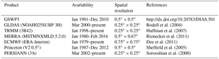
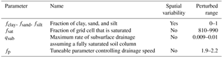
Table 2Model parameters that are sensitive to SM and GWS estimates. The following parameters were perturbed using the additive noise with the boundary conditions given in the last column. The further parameter description can be found in Decker (2015) and Ukkola et al. (2016).
CABLE is initially forced with the data from the Global Soil Wetness Project Phase 3 (GSWP3), which is currently available until December 2010 (http://hydro.iis.u-tokyo.ac.jp/GSWP3, https://doi.org/10.20783/dias.501). We replace GSWP3 forcing data with GLDAS data (Rodell et al., 2004) to compute the water storage changes to 2016. The forcing data used in CABLE are precipitation, air temperature, snowfall rate, wind speed, humidity, surface pressure, and short-wave and long-wave downward radiations. To investigate the impact of different forcing data, the offline sensitivity study is conducted by comparing the water storage estimates computed using
-
all eight forcing data components of GSWP3 and
-
GSWP3 data with the replacement of one component obtained from GLDAS forcing data.
It is found that the water storage estimate is most sensitive to the replacement of precipitation data, as expected, and relatively less sensitive to the change in other forcing components. We use the GLDAS forcing data in this study and also further test seven different precipitation data products (see more details in Sect. 4.2). The forcing data are up- or downsampled to a 0.5∘ × 0.5∘ spatial grid to reconcile with the CABLE spatial resolution.

Figure 2Histograms of the model errors computed from 210 ensemble members () without the mean. The basin averaged values (from all 10 Australian basins) of January 2003, for example, are shown.
4.2 Model uncertainty
In this study, the CABLE uncertainty is derived from 210 ensemble estimates associated with different forcing data and model parameters. The seven different precipitation products (see Table 1) are used to run the model independently. Most products are available to present day while GSWP3, Princeton, and MERRA are only available until December 2010, December 2012, and February 2016, respectively. For each precipitation forcing, 30 ensembles are generated by perturbing the model parameters within ±10 % of the nominal values. The perturbed size of 10 % is similar to Dumedah and Walker (2014). Based on the CABLE structure, the ΔSM and ΔGWS estimates are most sensitive to the model parameters listed in Table 2. For example, the fractions of clay, sand, and silt (fclay, fsand, fsilt) are used to compute soil parameters including field capacity, hydraulic conductivity, and soil saturation which mainly affect soil moisture storage. Similarly, the drainage parameters (e.g. qsub, fp) control the amount of subsurface runoff, which has a direct impact on root zone soil moisture and groundwater storages.
From ensemble generations, total K = 210 sets of the ensemble water storage estimates (he) are obtained:
and the mean value of 𝓗R is computed as follows:
Note that due to the absence of GSWP3, Princeton, and MERRA data, the number of ensembles reduces to K = 180 after December 2010, K = 150 after December 2012, and K = 120 after February 2016, respectively. The GC approach assumes that model errors are normally distributed with zero mean. Any violation of this assumption will yield a bias in the combined solutions. Therefore, the mean value is removed from each ensemble member, = 𝓗R − , and the error covariance matrix of the model is empirically computed as
The (Eq. 16) and CR (Eq. 17) terms can be directly used in Eq. (9). The distribution of model errors is demonstrated in Fig. 2. The figure illustrates the histogram of model errors () computed using 210 ensemble members of the model-estimated ΔSM and ΔGWS in January 2003. The histogram indicates that the model error may be approximately described by a normal distribution as introduced in Eq. (1).
Furthermore, in practice, the sampling error caused by finite sample size might lead to spurious correlations in the model covariance matrix (Hamill et al., 2001). The effect can be reduced by applying an exponential decay with a particular spatial correlation length to CR. In this study, the correlation length is determined based on the empirical covariance of model-estimated ΔTWS. The covariance function of ΔTWS is firstly assumed isotropic, and it is computed empirically based on the method given in Tscherning and Rapp (1974). The distance where the maximum value of the variance decreases to half is defined as the correlation length. The obtained values vary month to month, and the mean value of 250 km is used in this study.
It is emphasized that the model omission error caused by imperfect modelling of hydrological processes within the LSM is not taken into account in the above description. The omission error may increase the model covariance and introduce a bias as well. We account for the omission error by increasing 20 % of the model covariance. (i.e. multiplying CR by 1.2). We determine such omission error based on trial and error such that it increases the model error (due to the omission error) but does not exceed the model error value reported by Dumedah and Walker (2014). We acknowledge that this is only a simple practical way of accounting for the omission error into the total model error.
4.3 Validation data
4.3.1 Satellite soil moisture observation
The satellite-observed surface soil moisture data are obtained from the Advanced Microwave Scanning Radiometer aboard the Earth Observing System using the Land Parameter Retrieval Model (Njoku et al., 2003). The observation is used to validate our estimates of top soil moisture changes (ΔSMtop). The AMSR-E product provides volumetric water content in the top layer derived from a passive microwave data (from NASA EOS Aqua satellite) and forward radiative transfer model. In this study, the level 3 product, available daily between June 2002 and June 2011 at 0.25∘ × 0.25∘ spatial resolution, is used (Owe et al., 2008). The measurements from ascending and descending overpasses are averaged for each frequency band (C and X). Then, the monthly mean value is computed by averaging the daily data within a month. To obtain the variation in the surface soil moisture, the long-term mean between June 2002 and June 2011 is removed from the monthly data. Regarding the different depth measured in CABLE and AMSR-E, the cumulative density function (CDF)-matching technique (Reichle and Koster, 2004) is used to reduce the bias between the top soil moisture model and the observation. The CDF is built using the 2003–2004 data, and it is used for the entire period. There are no satellite-observed or ground-measured root zone soil moisture data for meaningful comparison with our results, particularly on a continental scale. Validation of ΔSMrz on regional and continental scales is currently unachievable due to a complete lack of observations on this spatial scale.
4.3.2 In situ groundwater
The in situ groundwater levels from bore measurements are obtained from two different ground observation networks (see Fig. 1). The data in Queensland are obtained from the Department of Natural Resources and Mines (DNRM) while the data in Victoria are from the Department of Environment and Primary Industries (DWPI). More than 10 000 measurements are available from each network, but the data gap and outliers are present. Therefore, the bore measurement is firstly filtered by removing the sites that present no data or data gap longer than 30 months during the study period.
To obtain the monthly mean value, the hourly or daily data are averaged in a particular month. The outliers are detected and fixed using the Hampel filter (Pearson, 2005) where the remaining data gaps are filled using the cubic spline interpolation. To obtain the groundwater level variation, the long-term mean groundwater level computed between the study period is removed from the monthly values. The groundwater level variation (ΔL) is then converted to ΔGWS using ΔGWS = Sy ⋅ ΔL, where Sy is specific yield. Based on Chen et al. (2016), Sy = 0.1 is used for the Victoria network. Specific yields of Queensland's network have been found ranging from 0.045 (Rassam et al., 2013) to 0.06 (Welsh, 2008), and an averaged Sy = 0.05 is used in this study. Finally, the mean value computed from all data (in each network) is used to represent the in situ data of the network.
5.1 Model-only performance
We study the model ΔTWS changes under different meteorological forcing and land parameterization. A total of 210 estimates of monthly TWS (sum of SMtop, SMrz, and GWS) are obtained between January 2003 and March 2016 from the ensemble run based on seven different precipitation inputs. Then, the averaged values of the TWS estimates are computed from the 30 precipitation-associated ensemble members. This results in seven sets of monthly mean TWS estimates from seven different precipitation data. For each set, the monthly ΔTWS is computed by removing the long-term mean computed between January 2003 and March 2016.
The precipitation-based ΔTWS values are then compared with the GRACE mascon solution (see Sect. 3.2) over 10 different Australian basins. The comparison is carried out between January 2003 and March 2016. Due to the availability of the data, the periods used are shorter in cases of GSWP3, Princeton, and MERRA precipitation (see Table 1). The metric used to evaluate a goodness of fit between the CABLE run and GRACE mascon estimates is the Nash–Sutcliffe (NS) coefficient (see Eq. B1) (Fig. 3).
Figure 3 demonstrates CABLE ΔTWS varies noticeably by precipitation as well as locations. The area-weighted average values (see Eq. B2) computed from Princeton, GSWP3, and TRMM yield the model ΔTWS, reasonably agreeing with GRACE by giving an NS coefficient greater than 0.45, while MERRA, PERSIANN, and GLDAS show NS = ∼ 0.3. The lower agreement is mainly due to the quality of rainfall estimates over Australia. The NS of ECMWF is around 0.4.
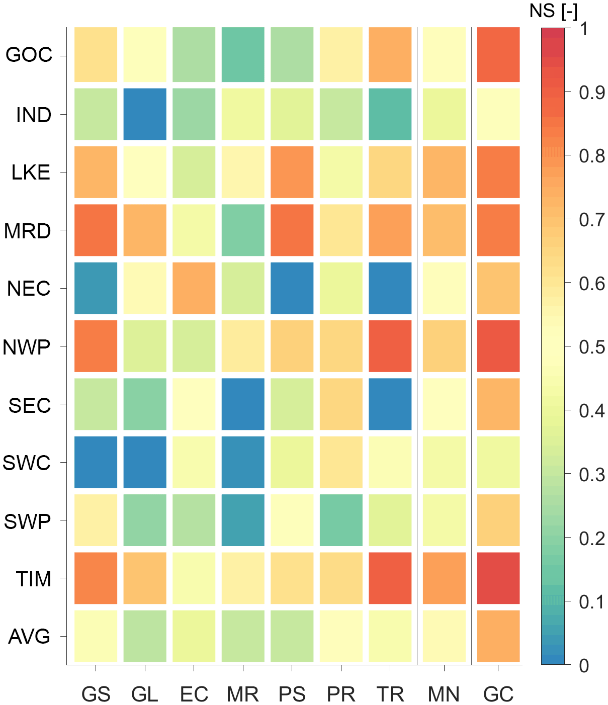
Figure 3NS coefficients between the model and GRACE mascon ΔTWS over 10 Australian basins (in ordinate). The NS values were computed based on CABLE ΔTWS computed with seven different precipitation data (in abscissa), including GSWP3 (GS), GLDAS (GL), ECMWF (EC), MERRA (MR), PERSIANN (PR), TRMM (TR). The NS value of the mean ΔTWS estimates (the average of seven variants) is also shown (MN). The area-weighted average NS value over all basins is also shown (AVG). The NS value of ΔTWS from the GRACE-combined (GC) approach is shown in the last column. The full name of the basins can be found in Fig. 1.
All model ensembles are consistent with the GRACE data over the Timor Sea and inner parts of Australia (e.g. Lake Eyre, LKE; Murray–Darling, MRD; North West Plateau, NWP) where the NS value can reach as high as 0.9 (see e.g. TRMM over TIM, Timor Sea). On the contrary, the lower agreement is found mostly over the coastal basins. Very small or even negative NS values indicate the misfit between the CABLE and GRACE mascon solutions, and they are observed over the Indian Ocean (see GLDAS), North East Coast (NEC; see GSWP3, PERSIANN, TRMM), South East Coast (see MERRA, TRMM), South West Coast (SWC; see GSWP3, GLDAS, MERRA), and South West Plateau (SWP; see MERRA).
By averaging all ΔTWS estimates from seven different precipitation datasets, the mean-ensemble estimate (MN) delivers the best agreement with GRACE as seen by the highest average NS value (MN of AVG = 0.55) among all ensembles. Particularly, NS values are greater than 0.4 in all basins and no negative NS values are presented in MN. On average, it can be clearly seen that using the mean value (MN) is a viable option to increase the overall performance of the ΔTWS estimates. Therefore, only the CABLE MN result will be used in further analyses. The comparison with the GRGS GRACE solution was also evaluated (not shown here) and the overall results are similar to Fig. 3.
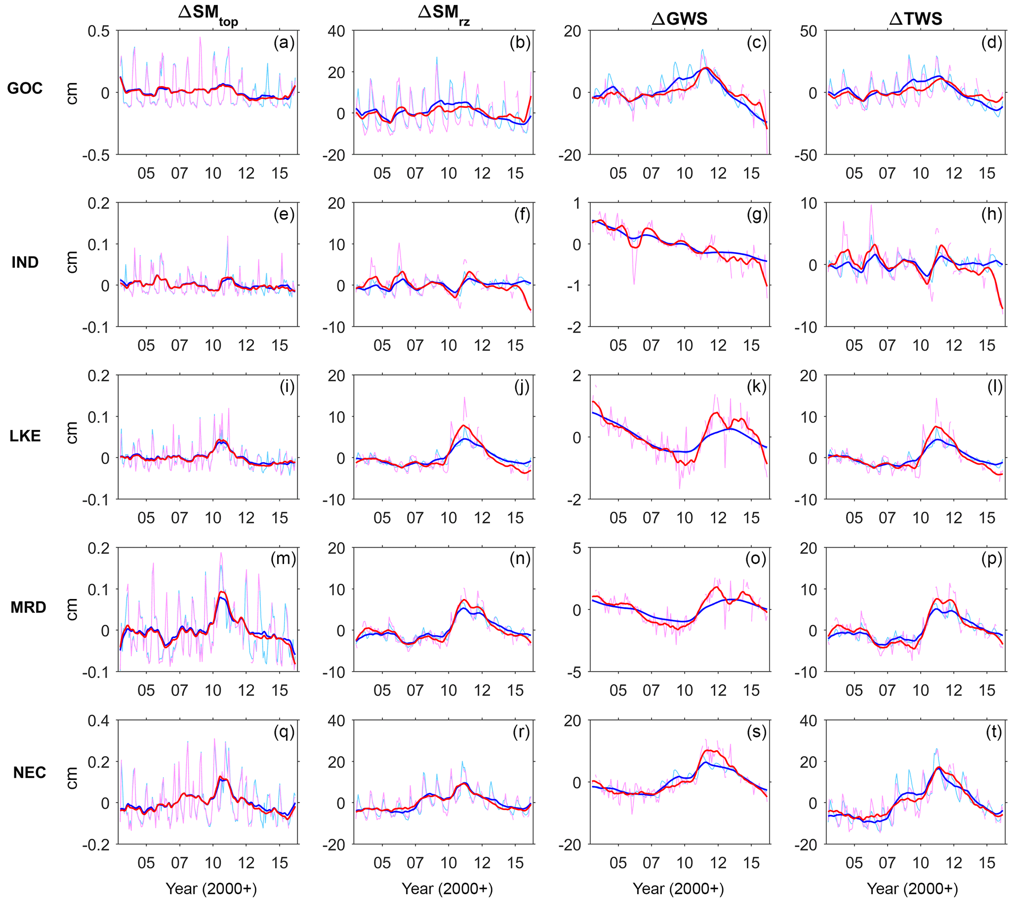
Figure 4The monthly time series of ΔSMtop, ΔSMrz, ΔGWS, and ΔTWS estimated from model (blue) and GC (red) solutions over the Gulf of Carpentaria (GOC), Indian Ocean (IND), Lake Eyre (LKE), Murray–Darling (MRD), and North East Coast (NEC). The deseasonalized time series is also shown.
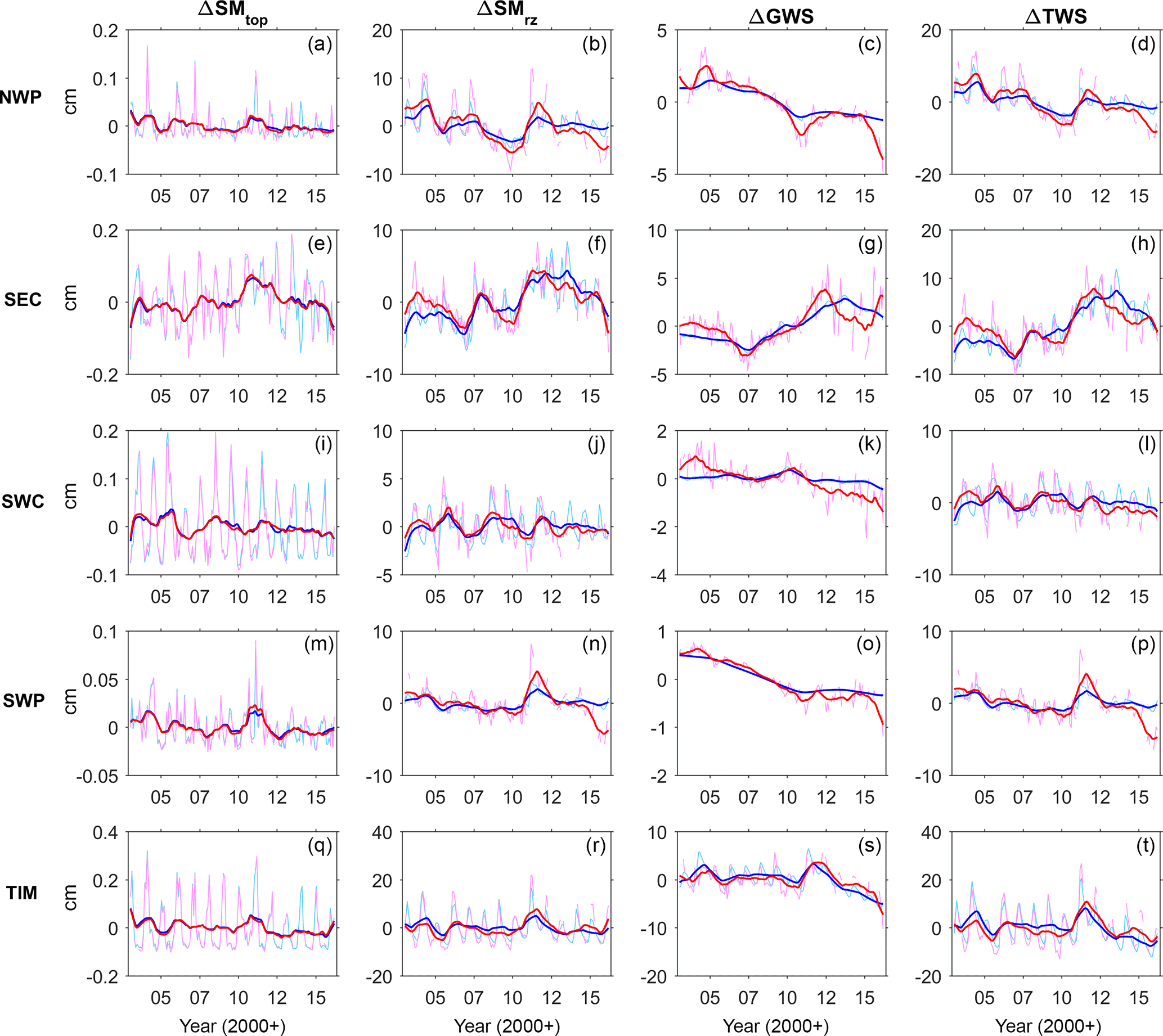
Figure 5Similar to Fig. 3, but estimated over the North West Plateau (NWP), South East Coast (SEC), South West Coast (SWC), South West Plateau (SWP), and Timor Sea (TIM).
5.2 Impact of GRACE on storage estimates
5.2.1 Contribution of GRACE
This section investigates the impact of the GC approach on the estimates of various water storage components. The ΔTWS estimate obtained from the GC approach is demonstrated in Sect. 5.1, by comparing with the independent GRACE mascon solution. Figure 3 shows the GC result yields the highest NS values in all basins, outperforming all other CABLE runs. In the average (AVG), the NS value increases by ∼ 35 % (0.55 to 0.74) from the MN case. Similar behaviour is also seen when compared with the GRGS GRACE solution (not shown); the average NS value increases from 0.50 to 0.74. This is not surprising as the GC approach uses the fundamental GRACE tracking data as GRACE mascon and GRGS solutions do. Improvement of the NS coefficient indicates merely the successfulness of integrating GRACE data and the model estimates.
Figures 4 and 5 show the GC results of ΔTWS as well as ΔSMtop, ΔSMrz, and ΔGWS in different basins. The monthly time series and the deseasonalized time series are shown. In general, GRACE tends to increase ΔTWS when the model ΔTWS (MN) is predicted to be underestimated (see e.g. LKE, MRD, NWP, SWP, TIM between 2011 and 2012) and decrease ΔTWS when it is determined to be overestimated (see all basins between 2008 and 2010). A clear example is seen over the Gulf of Carpentaria (GOC, Fig. 4d), where CABLE overestimates ΔTWS and produces phase delay between 2008 and 2010. The overestimated amplitude and phase delay seen in CABLE ΔGWS during this above period (Fig. 4c) is caused by an overestimation of soil and groundwater storage. The positively biased soil and groundwater storage causes a phase delay by increasing the amount of time required for the subsurface drainage (baseflow) to reduce to soil and groundwater stores. The overestimation of water storage is the result of overestimated precipitation or underestimated evapotranspiration. The amplitude and phase of the water storage estimate are adjusted toward GRACE observation in the GC approach.
The impact of GRACE varies across the individual storage as well as across the geographical location (climate regime). In general, the major contributors to ΔTWS are ΔSMrz and ΔGWS. Due to a small store size (only ∼ 2 cm thick), ΔSMtop contributes only ∼ 2 % to ΔTWS. As such, ΔSMrz and ΔGWS have greater variations, which commonly lead to greater uncertainty compared to ΔSMtop, and, therefore, the stores anticipate greater shares from the GRACE update. This behaviour is seen over all basins where the differences between the CABLE-simulated and GC ΔSMrz, and ΔGWS estimates are greater (compared to ΔSMtop).
Furthermore, the impact of GRACE on ΔSMrz and ΔGWS is different across the continent. For example, over central and southern Australia (see e.g. LKE, MRD, NWP, SWP), the dry climate is responsible for a small amount of groundwater recharge and most of the infiltration is stored in soil compartments. In this climate condition, ΔSMrz amplitude is significantly larger than ΔGWS and it plays a greater role in ΔTWS, and, consequently, the GRACE contribution is mostly seen in the ΔSMrz component. Different behaviour is seen over northern Australia (GOC, NEC, TIM) where ΔGWS amplitudes are greater (∼ 40 % of ΔTWS) compared to other basins (only ∼ 17 % of ΔTWS). This is due to the sufficient amount of rainfall over the wet climate region, replenishing groundwater recharges and resulting in greater variability in ΔGWS. Therefore, compared to the dry climate basin, GRACE contributes to ΔGWS over these basins by a larger amount.
5.2.2 Impact on long-term trend estimates
The spatial patterns of the long-term trends of water storage changes over January 2003 and March 2016 are analysed before and after applying the GC approach (Fig. 6). For comparison, the long-term trends of ΔTWS derived from the ITSG-DDK5, mascon, and GRGS solutions are shown in Fig. 7. From Fig. 6b, GRACE effectively changes the long-term trend estimates in most basins in a way the spatial pattern of the ΔTWS trend of the GC solution consistent to the GRACE solutions while satisfying the model processes and keeping the spatial resolution. The trend of ΔSMtop is insignificant (Fig. 6c) and the GC approach does not change (Fig. 6d). The largest adjustment is seen in ΔSMrz and ΔGWS components, to be consistent with the GRACE data in most basins (Fig. 6 and h).
GRACE shows significant changes in the ΔTWS trend estimates particularly over the northern and western parts of the continent (Fig. 7). The model estimates around the Gulf of Carpentaria basin show a strong negative trend that is inconsistent from the GRACE data. It is found that underestimated precipitation after 2012 is likely the cause of such an incompatible negative trend (see Fig. 4d). Applying the GC approach clearly improves the trend (Fig. 6a vs. Fig. 6b). The other example is seen over the western part of the continent (see rectangular area in Fig. 6a and b) where the averaged long-term trend of ΔTWS was predicted to be −0.4 cm yr−1 but changed to be −1.2 cm yr−1 (see also Sect. 5.4) by the GC approach. The precipitation over Western Australia is understood to be overestimated after 2012, evidently seen by the fact that the model ΔTWS is always greater than the GC solution (see e.g. Figs. 4h, 5d and p). The GC approach reveals that the water loss over Western Australia is at least 2 times greater than what has been predicted by the CABLE model.
In addition, the shortage of water storage in the south-eastern part of the continent from the Millennium Drought (McGrath et al., 2012) has been recovered (seen as a positive water storage trend in Fig. 6) after the rainfall between 2009 and 2012, while the western part is still drying out (seen as negative trends). The trend estimates in terms of mass change are discussed in more detail in Sect. 5.4.
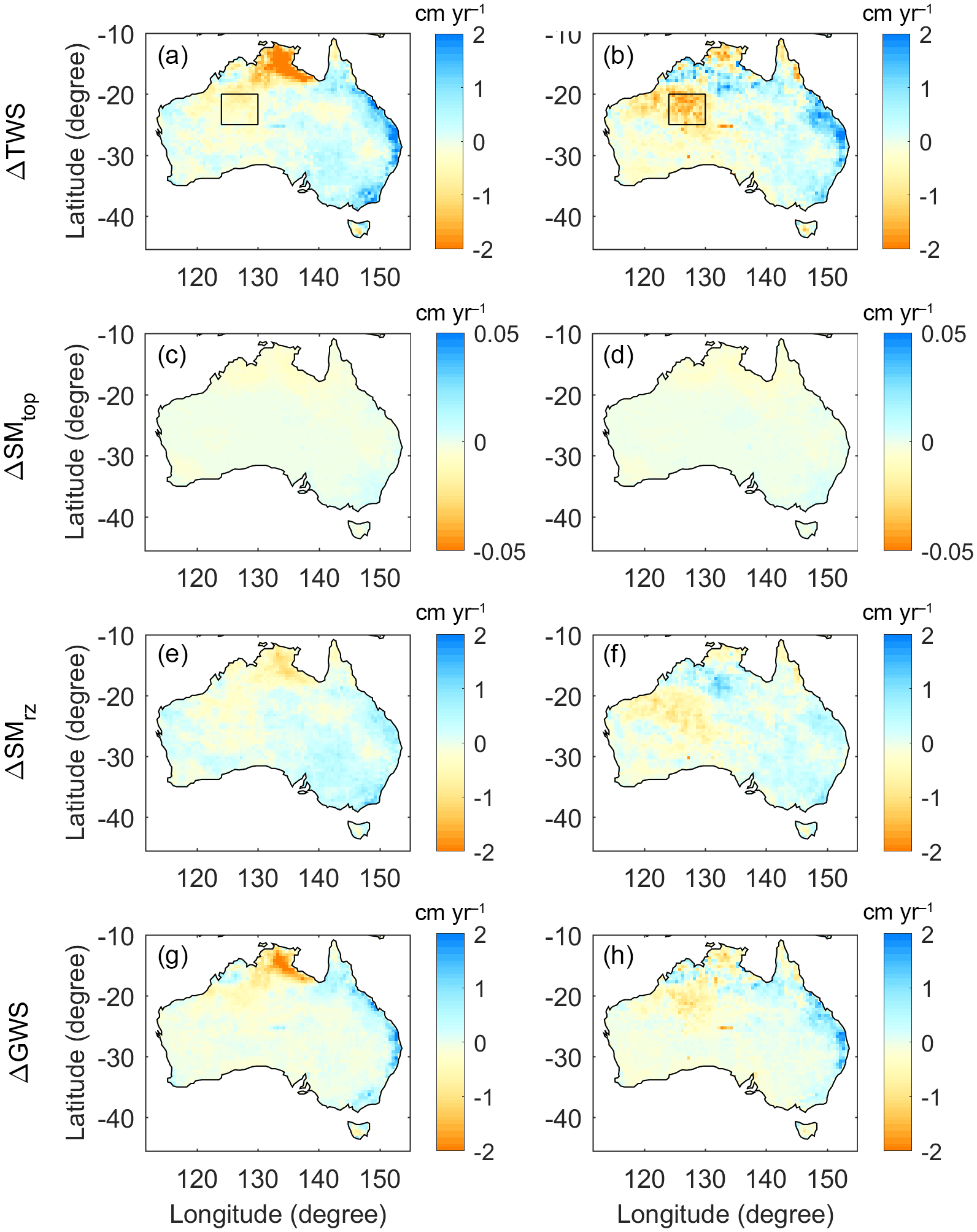
Figure 6Long-term trends of ΔTWS (a, b), ΔSMtop (c, d), ΔSMrz (e, f), and ΔGWS (g, h) estimated from the model-only (left) and the GC solutions (right). The eastern part of North West Plateau basin is shown as a rectangle polygon in (a) and (b).
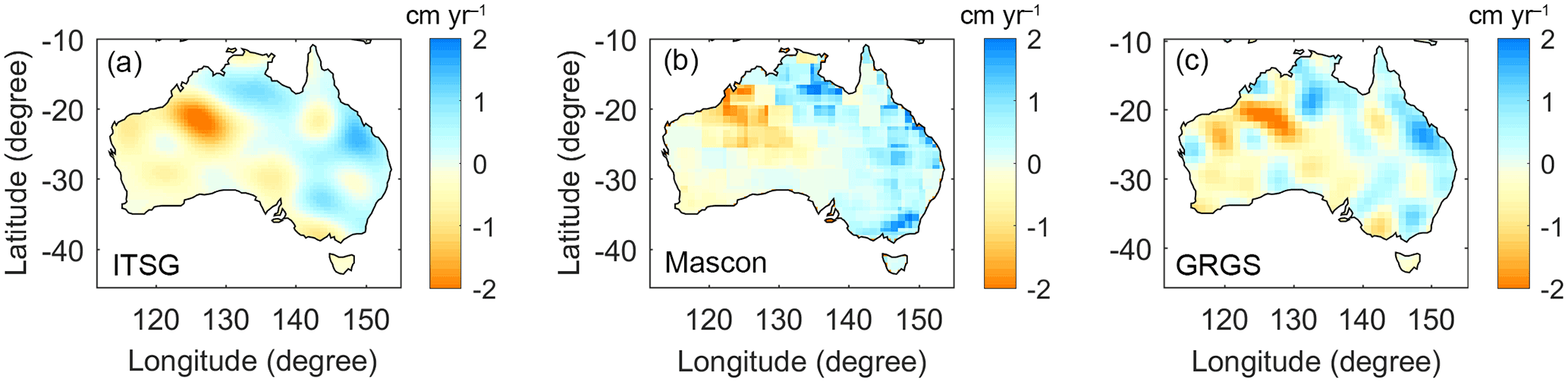
Figure 7Long-term trends of GRACE-derived ΔTWS from ITSG-DDK5 (a), mascon (b), and GRGS solution (c).

Figure 8Uncertainties in ΔSMtop, ΔSMrz, ΔGWS, and ΔTWS estimated from the model (blue) and the GC solutions (red) in 10 different Australian basins. The uncertainty in the precipitation is shown in (e). The area-weighted average value (AVG) is also shown.
5.2.3 Reduction of uncertainty
Influenced by climate pattern, the uncertainty in water storage estimates significantly varies across Australia. The uncertainty in the model estimate is computed from the variability induced by different precipitation and model parameters while the uncertainty in the GC solution is computed using Eq. (11). As expected, larger uncertainties are observed in ΔSMrz and ΔGWS than in ΔSMtop (an order of magnitude smaller) since ΔSMtop is smaller than others (Fig. 8). Over the wet basins, larger amplitude of the water storage leads to larger uncertainty, seen over the Gulf of Carpentaria, North East Coast, South East Coast, and Timor Sea where the CABLE-simulated ΔTWS uncertainty is approximately 28 % larger than other basins. The smaller uncertainty is found over the dry regions (e.g. LKE, SWP). In most basins, the uncertainty in ΔSMrz is larger than the ΔGWS, except the wet basins (e.g. GOC, NEC, TIM) where the greater groundwater recharge leads to a larger uncertainty in ΔGWS.
Figure 8 demonstrates how much the formal error of each of the storage components is reduced by the GC approach. Overall, the estimated CABLE uncertainties averaged over all basins (AVG) are 0.2, 4.0, 4.0, and 5.7 cm for ΔSMtop, ΔSMrz, ΔGWS, and ΔTWS, respectively. With the GC approach, the uncertainties in ΔSMtop, ΔSMrz, ΔGWS, and ΔTWS decrease by approximately 26, 35, 39, and 37 %, respectively.
It is worth mentioning that the model uncertainty is mainly influenced by the meteorological forcing data. The uncertainty in precipitation derived from seven different precipitation products is shown in Fig. 8e. The spatial pattern of the precipitation uncertainty is correlated with the uncertainty in water storage estimates. The larger water storage uncertainty is deduced from the larger precipitation uncertainty. The quality of precipitation forcing data is found to be an important factor to determine the accuracy of water storage computation.
5.3 Comparison with independent data
5.3.1 Soil moisture
The ΔSMtop estimates are compared with the AMSR-E-derived soil moisture. The processing of AMSR-E data is described in Sect. 4.3.1. The performance is assessed using Nash–Sutcliffe coefficients, given in Table 3. In general, CABLE (MN) shows a good performance in the top soil moisture simulation showing an NS value of > 0.4 for most of the basins. The top soil moisture estimate shows slightly better agreement with the C-band measurement of the AMSR-E product. This is likely caused by the greater emitting depth of the C-band measurement (∼ 1 cm), which is closer to the depth of the top soil layer (∼ 2 cm) used in this study (Njoku et al., 2003).
The GC approach leads to a small bit of improvement of the top soil estimate consistently from C- and X-band measurements and from all basins. No degradation of the NS value is observed in the GC solutions. The largest improvement is seen over LKE and NEC, where NS increases by 10–15 %. For other regions, the change in the NS coefficient may be incremental.
5.3.2 Groundwater
The ΔGWS estimates from the model and the GC method are compared with the in situ data obtained from two different ground networks in Queensland and Victoria. For each network, all ΔGWS data inside the groundwater network boundary (see polygons in Fig. 1) are used to compute the average ΔGWS time series. From the comparison given in Fig. 9, it is found that the GC solutions of ΔGWS follow the overall inter-annual pattern of CABLE but with a considerably larger amplitude. This results in a better agreement with the in situ ΔGWS data seen from both networks. The NS coefficient of ΔGWS between the estimates and the in situ data are given in Table 4. The CABLE ΔGWS performs significantly better in Queensland (NS = ∼ 0.5) than Victoria (NS = ∼ 0.3). Significant improvement is found from the GC solutions in both networks, where the NS value increases from 0.5 to 0.6 (∼ 22 %) in Queensland and from 0.3 to 0.6 (∼ 85 %) in Victoria. Even greater improvement is seen when the inter-annual patterns are compared. The NS value increases from 0.5 to 0.7 (∼ 32 %) and 0.4 to 0.8 (∼ 93 %) in Queensland and Victoria, respectively.
Table 3NS coefficients between top soil moisture estimates and the satellite soil moisture observations from AMSR-E products over 10 different Australian basins. The area-weighted average value (AVG) is also shown.
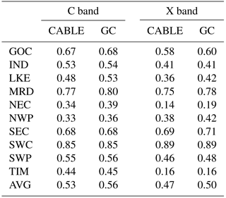
Table 4NS coefficient and long-term trend of ΔGWS estimated from the model-only and GC solutions in Queensland and Victoria groundwater network. The long-term trend of the in situ data is also shown.
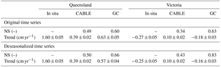
The comparison of the long-term trend of ΔGWS is also evaluated. The estimated trends in Queensland and Victoria are given in Table 4. Beneficially from the GC approach, the ΔGWS trend is improved by approximately 20 % (from 0.4 to 0.6, compared to 1.6 cm yr−1) in Queensland. The increase in ΔGWS is mainly influenced by the large amount of rainfall during the 2009–2012 La Niña episodes (see Fig. 9a). In Victoria, a significant improvement of the ΔGWS trend by about 76 % (from 0.1 to −0.2, compared to −0.3 cm yr−1) is observed. Similar improvement of long-term trend estimates is seen in deseasonalized time series (improves by ∼ 15 % in Queensland and by ∼ 74 % in Victoria). The decrease in ΔGWS in Victoria is mainly due to the highly demanded groundwater consumption by agriculture and domestic activities (Van Dijk et al., 2007; Chen et al., 2016). As the groundwater consumption is not parameterized in CABLE, the decrease in the ΔGWS estimate cannot be properly captured in the model simulation. Applying GC approach effectively reduces the model deficiency and improves the quality of the groundwater estimations.
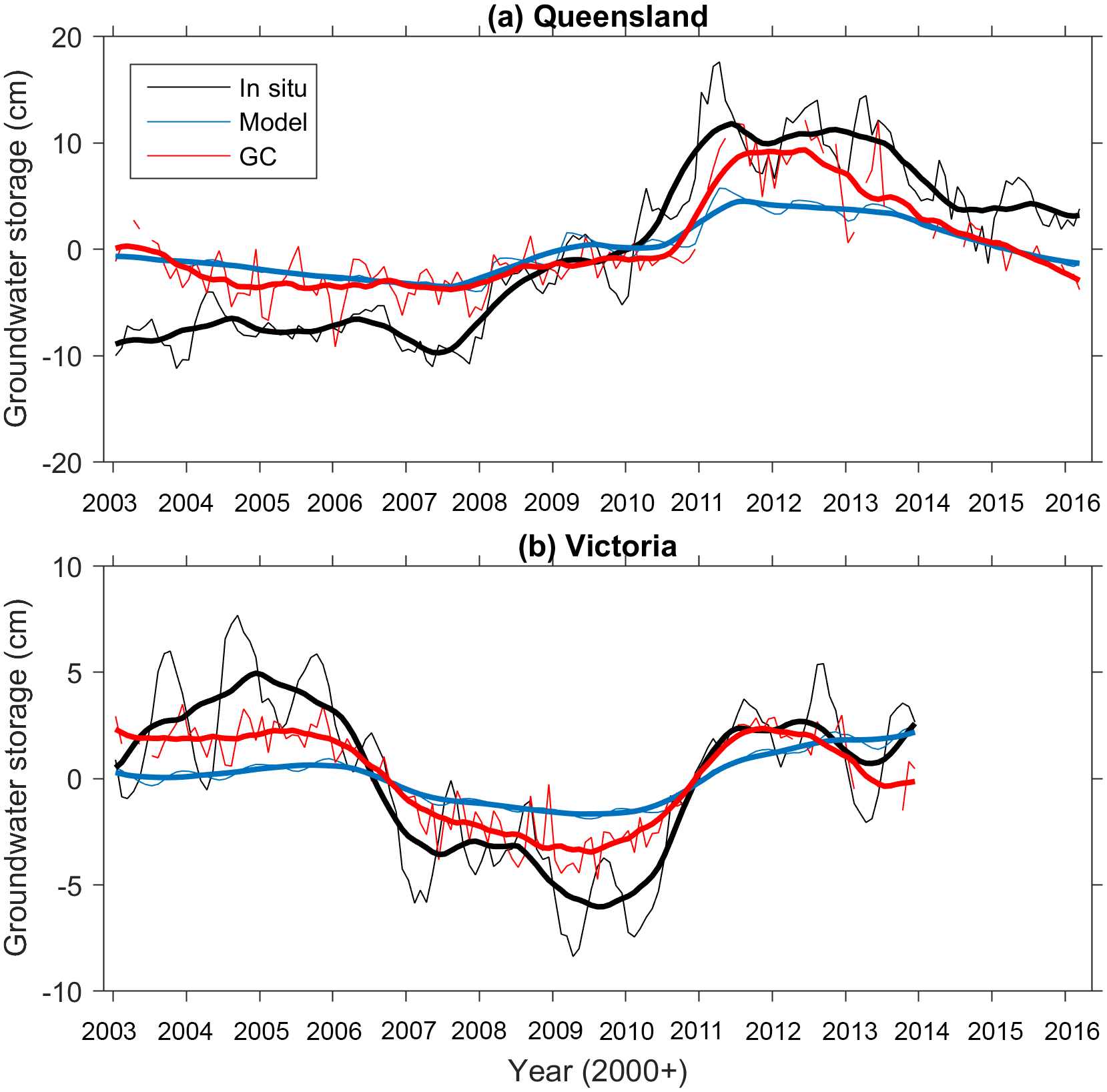
Figure 9The monthly time series of ΔGWS estimated from the model, GC solutions, and measured from the in situ groundwater network in Queensland (a) and Victoria (b). Deseasonalized time series are shown in thick lines.
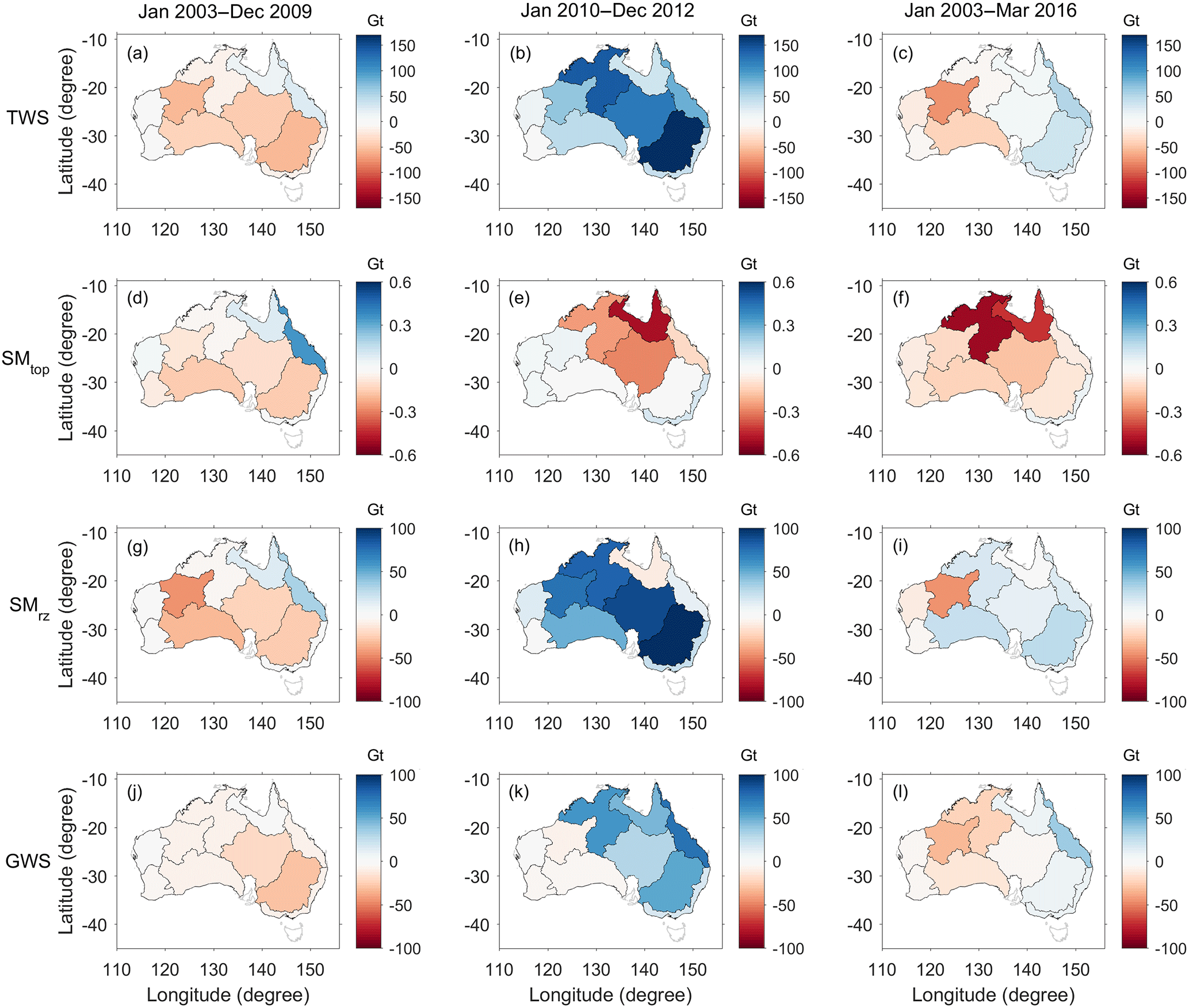
Figure 10Mass changes (Gt, Gigatonne) of ΔTWS, ΔSMtop, ΔSMrz, and ΔGWS estimated from GC solutions over 10 Australian basins in three different periods: Big Dry (January 2003–December 2009), Big Wet (January 2010–December 2012), and the entire period (January 2003–March 2016).
5.4 Assessment of mass variation in the past 13 years
Australia experiences significant climate variability; for example, the Millennium Drought starting from late 1990 (Van Dijk et al., 2013) and extremely wet conditions during several La Niña episodes (Trenberth, 2012; Han, 2017). These periods are referred as “Big Dry” and “Big Wet” (Ummenhofer et al., 2011; Xie et al., 2016). To understand the total water storage (mass) variation influenced by these two distinct climate variabilities, the water storage change obtained from the GC approach during Big Dry and Big Wet is separately investigated over 10 basins. The time window between January 2003 and December 2009 is defined as the Big Dry period while between January 2010 and December 2012 it is defined as the Big Wet period following Xie et al. (2016). In each period, the long-term trends of GC estimates of ΔTWS, ΔSMtop, ΔSMrz, and ΔGWS are firstly calculated. Then, the total water storage variation (in m) is simply obtained by multiplying the long-term trend (in m yr−1) with the number of years in the specific period – 7 years for Big Dry and 3 years for Big Wet. To obtain the mass variation, the water storage variation is multiplied by the area of the basin and the density of water (1000 kg m−3). The estimated mass variations during Big Dry and Big Wet are displayed in Fig. 10. The long-term mass variation in the entire period (January 2003–March 2016) is also shown.
During Big Dry (2003–2009), a significant loss of total storage (40–60 Gt over 7 years) is observed over the LKE, MRD, NWP, and SWP basins. The largest groundwater loss of > 20 Gt is found from LKE and MRD. No significant change is observed over the tropical climate regions (e.g. GOC, NEC). The mass loss mostly occurs in the root zone and groundwater compartments where the sum of ΔSMrz and ΔGWS explains more than 90 % of the ΔTWS value. The mass loss is also observed in ΔSMtop but is > 10 times smaller than ΔSMrz and ΔGWS.
During Big Wet (2010–2012), the basins such as LKE, MRD, and TIM exhibit the significant total storage gain of > 100 Gt. The gain is particularly larger in ΔSMrz over the basins that experienced the significant loss during Big Dry. For example, over LKE and MRD, the gain of ΔSMrz is approximately 2–3 times greater than ΔGWS. It implies that most of the infiltration (from the 2009–2012 La Niña rainfall) is stored as soil moisture through the long drought period and that the groundwater recharge is secondary to the ΔSMrz increase.
The opposite behaviour is observed over the basins (such as NEC and GOC) that experienced mass gain during Big Dry. The water storage gain is greater in ΔGWS compared to ΔSMrz. In NEC, ΔGWS gain is ∼ 8 times larger than ΔSMrz during Big Wet. The soil compartment may be saturated during Big Dry and additional infiltration from the Big Wet precipitation leads to an increased groundwater recharge. The ΔSMrz loss observed over GOC is simply caused by the timing selection of the Big Wet period, which ends earlier (∼ 2011) in GOC than in other basins. The ΔSMrz gain becomes ∼ 26 Gt if the Big Wet period is defined as 2008–2011. During the post-Big-Wet period (2012 and afterwards), the decreasing trend of water storage is observed from all basins (see Figs. 4 and 5). This is mainly caused by the decrease in precipitation after 2012 and by gradual water loss through evapotranspiration (Fasullo et al., 2013).
The overall water storage change in the last 13 years demonstrates that the severe water loss from most basins during Big Dry (the Millennium Drought) is balanced with the gain during Big Wet (the La Niña). The negative ΔTWS estimated during Big Dry becomes positive in LKE, MRD, and SEC and less negative in TIM, and the greatest gain is observed from NEC by ∼ 50 Gt during the 13-year period (see Fig. 10c). However, the water mass loss is still detected over the western basins (e.g. IND, NWP, SWP, SWC), and their magnitudes are even larger than the mass loss during Big Dry. For example, the greatest ΔTWS loss of ∼ 79 Gt is observed over NWP, which is ∼ 25 Gt greater than the loss during Big Dry (see Fig. 10a and c). The basin is less affected by the La Niña, and the rainfall during Big Wet is clearly inadequate to support the water storage recovery in the basin. Rainfall deficiency also reduces the groundwater recharge, resulting in even more decreasing of ΔGWS, compared to the Millennium Drought period (see Fig. 10j and l). The continual decrease in water storage over western basins is likely caused by the interaction of complex climate patterns such as the El Niño–Southern Oscillation, Indian Ocean Dipole, and Southern Annular Mode cycles (Australian Bureau of Meteorology, 2012; Xie et al., 2016).
5.5 Comparison of the GC approach with alternatives
The simplest approach to estimate ΔGWS is to subtract the model soil moisture component from GRACE ΔTWS data, without considering uncertainty in the model output, as used in Rodell et al. (2009) and Famiglietti et al. (2011). This method is called Approach 1 (App 1). In Approach 2 (App 2) as in Tangdamrongsub et al. (2017), by accounting for the uncertainty in model outputs and GRACE data, the water storage states are updated through a Kalman filter:
where , H, CR are described in Sect. 2; b is an observation vector containing GRACE-derived ΔTWS; and R is an error variance–covariance matrix of the observation. The GRACE-derived ΔTWS and its error information is obtained from the mascon solution. The matrix R is a (diagonal) error variance matrix since no covariance information is given in the mascon product. Note that the model uncertainty remains the same as in GC approach (Sect. 4.2). The different results from App 1 and App 2 are mainly attributed to the different estimates of the uncertainty.
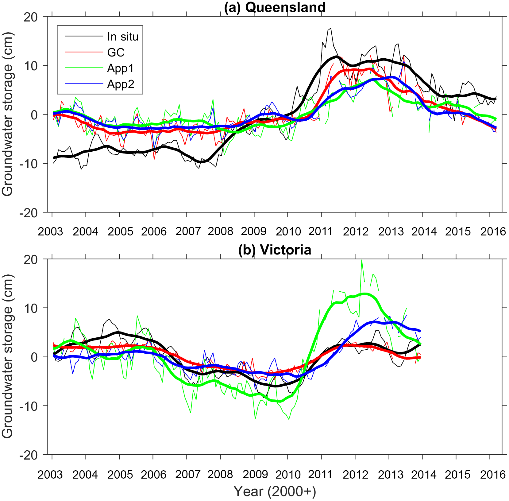
Figure 11ΔGWS estimated from Approach 1 (App 1) and Approach 2 (App 2) in Queensland (a) and Victoria (b). The in situ groundwater network data and the GC solutions are also shown. Deseasonalized time series are shown in thick lines.
The ΔGWS estimates from App 1, App 2, and GC in Queensland and Victoria are shown in Fig. 11. It is clearly seen that ΔGWS values from App 1 are overestimated while the one from App 2 fits the ground data significantly better. This behaviour was also seen in Tangdamrongsub et al. (2017), where the water storage estimates tend to be overestimated when error components such as spatial correlation error were neglected as in App 1. ΔGWS from App 2 shows clear improvements in terms of NS coefficients in both networks. Considering the deseasonalized ΔGWS estimates, in Queensland, the trend increases from 0.39 ± 0.03 to 0.42 ± 0.03 cm yr−1 (improves by 1.5 %) and the NS value increases from 0.46 to 0.53. In Victoria, the trend decreases from 0.73 ± 0.10 to 0.46 ± 0.05 cm yr−1 (improves by 27 %) and the NS value increases from −0.89 to 0.30. Although App 2 is not yet as good as the GC solution based on the most comprehensive error propagation, this simple test demonstrates the importance of considering the uncertainty. The reason for App 2 being less accurate than GC is likely the too-simplified error information implemented in App 2.
This study presents an approach to combine the raw GRACE observation with model simulation to improve water storage estimates over Australia. Distinct from other methods, we exploit the fundamental GRACE satellite tracking data and the full data error variance–covariance information to avoid alteration of signal and measurement error information present in higher-level data products.
We compare groundwater storage estimates from the GC approach and two other approaches, subject to inclusion of GRACE uncertainty in the ΔGWS calculation. Validating three results of ΔGWS against the in situ groundwater data, we find that the GC approach delivers the most accurate groundwater estimate, followed by the approach based on incomplete information of GRACE's data error. The poorest estimate of groundwater storage is seen when the GRACE uncertainty is completely ignored. This confirms the critical value of using the complete GRACE signal and error information at the raw data level.
The analysis of water storage change between 2003 and 2016 reveals that half of the continent (5 out of 10 basins) has still not fully recovered from the Millennium Drought. The TWS decrease in Western Australia has been most characteristic, and the GC approach finds that the water loss mainly occurs in the groundwater layer. Rainfall inadequacy is attributed to the continual dry condition, leading to a greater decrease in groundwater recharge and storage over Western Australia.
The land surface model we used is deficient in anthropogenic groundwater consumption. The model calibration will never help, and the groundwater consumption must be brought in by external sources. On the contrary, statistical approaches similar to our GC approach may be useful to fill in the missing component and lead to a more comprehensive water storage inventory.
However, it is difficult to constrain different water storage components by only using total storage observation such as GRACE. In addition, it is challenging to improve surface soil moisture varying rapidly in time, using a monthly mean GRACE observation. Tian et al. (2017) utilized the satellite soil moisture observation from Soil Moisture and Ocean Salinity (SMOS, Kerr et al., 2001) in addition to GRACE data for their data assimilation and showed a clear improvement in the top soil moisture estimate. The GC approach with complementary observations at higher temporal resolution should be considered, particularly to enhance the surface soil moisture computation.
Furthermore, the GC approach can be simply extended for GRACE data assimilation. Assimilating the raw GRACE data into land surface models like CABLE enables the model state and parameter to be adjusted with the realistic error information, allowing more reliable storage computation.
This study is based on third-party data. The data providers are acknowledged in the data sections (Sects. 3 and 4). The CABLE model can be obtained after registration at https://trac.nci.org.au/trac/cable.
A linearized GRACE satellite-tracking observation equation is formulated as
where y is the observation vector containing various kinds of L1B data including the inter-satellite ranging data; A is the design (partial derivative) matrix relating the data and the Earth gravity field variations; x contains the Stokes coefficients of time-varying geopotential fields (e.g. Wahr et al., 1998); and e is the L1B data noise, which has zero mean and covariance Σ. Equation (A1) can be modified explicitly in terms of soil moisture and groundwater storage variations as
where S contains a factor used to convert ΔTWS to geopotential coefficients considering the load Love numbers (e.g. Wahr et al., 1998) and converts the gridded data into the corresponding spherical harmonic coefficients. For convenience, the term Y = is used in the further derivation. A least-squares solution of Eq. (A2) is given as
It can be simplified as
where N = ATΣ−1A and c = ATΣ−1y. Equation (A4) is identical to Eq. (5).
The Nash–Sutcliffe coefficient (NS) is computed as follows:
where y is an observation vector, is the mean of the observation, is a vector containing the simulated result, i is the index of observation, and N is the number of observations.
Area-weighted average () is compute as follows:
where w is the area size, is the mean value inside the considered area, j is the area index, and M is the number of considered areas.
The authors declare that they have no conflict of interest.
This work is funded by The University of Newcastle to support NASA's GRACE
and GRACE Follow-On projects as an international science team member to the
missions. Mark Decker was supported by the ARC Centre of Excellence for Climate Systems
Science. Hyungjun Kim was supported by Japan Society for the Promotion of Science
KAKENHI (16H06291). We thank Torsten Mayer-Gürr for GRACE data products
in the form of the least-squares normal equations. We also thank three
anonymous reviewers for helping us improve the manuscript.
Edited by: Louise Slater
Reviewed by: three anonymous referees
Australian Bureau of Meteorology: Record-breaking La Niña events: An analysis of the La Niña life cycle and the impacts and significance of the 2010–11 and 2011–12 La Niña events in Australia, National Climate Centre, Bureau of Meteorology, http://www.bom.gov.au/climate/enso/history/La-Nina-2010-12.pdf (last access: 5 January 2017), 2012.
Bettadpur, S.: CSR Level-2 Processing Standards Document for Product Release 05, GRACE 327-742, Center for Space Research, The University of Texas, Austin, 2012.
Chen, J. L., Wilson, C. R., Tapley, B. D., Scanlon, B., and Güntner, A.: Long-term groundwater storage change in Victoria, Australia from satellite gravity and in situ observations, Global Planet. Change, 139, 56–65, https://doi.org/10.1016/j.gloplacha.2016.01.002, 2016.
Decker, M.: Development and evaluation of a new soil moisture and runoff parameterization for the CABLE LSM including subgrid-scale processes, J. Adv. Model. Earth Syst., 7, 1788–1809, https://doi.org/10.1002/2015MS000507, 2015.
Dee, D. P., Uppala, S. M., Simmons, A. J., Berrisford, P., Poli, P., Kobayashi, S., Andrae, U., Balmaseda, M. A., Balsamo, G., Bauer, P., Bechtold, P., Beljaars, A. C. M., van de Berg, L., Bidlot, J., Bormann, N., Delsol, C., Dragani, R., Fuentes, M., Geer, A. J., Haiberger, L., Healy, S. B., Hersbach, H., Hólm, E. V., Isaksen, L., Kållberg, P., Köhler, M., Matricardi, M., McNally, A. P., Monge-Sanz, B. M., Morcrette, J. J., Park, B. K., Peubey, C., de Rosnay, P., Tavolato, C., Thépaut, J. N., and Vitart, F.: The ERA-Interim reanalysis: configuration and performance of the data assimilation system, Q. J. Roy. Meteorol. Soc., 137, 553–597, https://doi.org/10.1002/qj.828, 2011.
Dumedah, G. and Walker, J. P.: Intercomparison of the JULES and CALBE land surface models through assimilation of remote sensed soil moisture in southeast Australia, Adv. Water Resour., 74, 231–244, https://doi.org/10.1016/j.advwatres.2014.09.011, 2014.
Eicker, A., Schumacher, M., Kusche, J., Döll, P., and Müller Schmied, H.: Calibration data assimilation approach for integrating GRACE data into the WaterGAP Global Hydrology Model (WGHM) using an Ensemble Kalman Filter: First Results, Surv. Geophys., 35, 1285–1309, https://doi.org/10.1007/s10712-014-9309-8, 2014.
Famiglietti, J. S., Lo, M., Ho, S. L., Bethune, J., Anderson, K. J., Syed, T. H., Swenson, S. C., de Linage, C. R., and Rodell, M.: Satellites measure recent rates of groundwater depletion in California's Central Valley, Geophys. Res. Lett., 38, L03403, https://doi.org/10.1029/2010GL046442, 2011.
Fasullo, J. T., Boening, C., Landerer, F. W., and Nerem, R. S.: Australia's unique influence on global sea level in 2010–2011, Geophys. Res. Lett., 40, 4368–4373, https://doi.org/10.1002/grl.50834, 2013.
Girotto, M., De Lannoy, G. J. M., Reichle, R. H., and Rodell, M.: Assimilation of gridded terrestrial water storage observations from GRACE into a land surface model, Water Resour. Res., 52, 4164–4183, https://doi.org/10.1002/2015WR018417, 2016.
Hamill, T. M., Whitaker, J. S., and Snyder, C.: Distance-Dependent Filtering of Background Error Covariance Estimates in an Ensemble Kalman Filter, Mon. Weather Rev., 129, 2776–2790, 2001.
Han, S.-C.: Elastic deformation of the Australian continent induced by seasonal water cycles and the 2010–11 La Niña determined using GPS and GRACE, Geophys. Res. Lett., 44, 2763–2772, https://doi.org/10.1002/2017GL072999, 2017.
Huffman, G. J., Adler, R. F., Bolvin, D. T., Gu, G., Nelkin, E. J., Bowman, K. P., Hong, Y., Stocker, E. F., and Wolf, D. B.: The TRMM multisatellite precipitation analysis (TMPA): Quasi-global, multiyear, combined-sensor precipitation estimates at fine scales, J. Hydrometeorol., 8, 38–55, https://doi.org/10.1175/JHM560.1, 2007.
Jekeli, C.: Alternative methods to smooth the Earth's gravity field, Rep. 327, Dept. of Geod. Sci. and Surv., Ohio State Univ., Columbus, 1981.
Kerr, Y. H., Waldteufel, P., Wigneron, J.-P., Martinuzzi, J.-M., Font, J., and Berger, M.: Soil moisture retrieval from space: The soil moisture and ocean salinity (SMOS) mission, IEEE T. Geosci. Remote, 39, 1729–1735, 2001.
Khaki, M., Hoteit, I., Kuhn, M., Awange, J., Forootan, E., van Dijk, A., Schumacher, M., and Pattiaratchi, C.: Assessing sequential data assimilation techniques for integrating GRACE data into a hydrological model, Adv. Water Resour., 107, 301–316, https://doi.org/10.1016/j.advwatres.2017.07.001, 2017a.
Khaki, M., Schumacher, M., Forootan, E., Kuhn, M., Awange, J., and van Dijk, A.: Accounting for spatial correlation errors in the assimilation of GRACE into hydrological models through localization. Adv. Water Resour., 108, 99–112, https://doi.org/10.1016/j.advwatres.2017.07.024, 2017b.
Kusche, J., Schmidt, R., Petrovic, S., and Rietbroek, R.: Decorrelated GRACE time-variable gravity solutions by GFZ, and their validation using a hydrological model, J. Geodesy, 83, 903–913, https://doi.org/10.1007/s00190-009-0308-3, 2009.
Lambert, A., Huang, J., van der Kamp, G., Henton, J., Mazzotti, S., James, T. S., Courtier, N., and Barr, A. G.: Measuring water accumulation rates using GRACE data in areas experiencing glacial isostatic adjustment: The Nelson River basin, Geophys. Res. Lett., 40, 6118–6122, https://doi.org/10.1002/2013GL057973, 2013.
Landerer, F. W. and Swenson, S. C.: Accuracy of scaled GRACE terrestrial water storage estimates, Water Resour. Res., 48, W04531, https://doi.org/10.1029/2011WR011453, 2012.
Lemoine, J. M., Bourgogne, S., Bruinsma, S., Gégout, P., Reinquin, F., and Biancale, R.: GRACE RL03-v2 monthly time series of solutions from CNES/GRGS, EGU2015-14461, EGU General Assembly 2015, Vienna, Austria, 2015.
Long, D., Chen, X., Scanlon, B. R., Wada, Y., Hong, Y., Singh, V. P., Chen, Y., Wang, C., Han, Z., and Yang, W.: Have GRACE satellites overestimated groundwater depletion in the Northwest India Aquifer?, Sci. Rep., 6, 24398, https://doi.org/10.1038/srep24398, 2016.
Mayer-Gürr, T., Behzadpour, S., Ellmer, M., Kvas, A., Klinger, B., and Zehentner, N.: ITSG-Grace2016 – Monthly and Daily Gravity Field Solutions from GRACE, GFZ Data Services, https://doi.org/10.5880/icgem.2016.007, 2016.
Mayer-Gürr, T., Pail, R., Gruber, T., Fecher, T., Rexer, M., Schuh, W.-D., Kusche, J., Brockmann, J.-M., Rieser, D., Zehentner, N., Kvas, A., Klinger, B., Baur, O., Höck, E., Krauss, S., and Jäggi, A.: The combined satellite gravity field model GOCO05s, EGU 2015, Vienna, 2015.
McGrath, G. S., Sadler, R.,Fleming, K., Tregoning, P., Hinz, C., and Veneklaas, E. J.: Tropical cyclones and the ecohydrology of Australia's recent continental-scale drought, Geophys. Res. Lett., 39, L03404, https://doi.org/10.1029/2011GL050263, 2012.
Njoku, E. G., Jackson, T. L., Lakshmi, V., Chan, T., and Nghiem, S. V.: Soil Moisture Retrieval from AMSR-E, IEEE T. Geosci. Remote, 41, 215–229, 2003.
Owe, M., de Jeu, R., and Holmes, T.: Multisensor historical climatology of satellite-derived global land surface moisture, J. Geophys. Res., 113, F01002, https://doi.org/10.1029/2007JF000769, 2008.
Pearson, E. K.: Mining imperfect data: Dealing with contamination and incomplete records, ProSanos Corporation, Harrisburg, Pennsylvania, https://doi.org/10.1137/1.9780898717884, 2005.
Ramillien, G., Cazenave, A., and Brunau, O., Global time variations of hydrological signals from GRACE satellite gravimetry, Geophys. J. Int., 158, 813–826, 2004.
Rassam, D. W., Peeters, L., Pickett, T., Jolly, I., and Holz, L.: Accounting for surfaceegroundwater interactions and their uncertainty in river and groundwater models: A case study in the Namoi River, Australia, Environ. Model. Softw., 50, 108–119, https://doi.org/10.1016/j.envsoft.2013.09.004, 2013.
Reichle, R. H. and Koster, R. D.: Bias reduction in short records of satellite soil moisture, Geophys. Res. Lett., 31, L19501, https://doi.org/10.1029/2004GL020938, 2004.
Rienecker, M. M., Suarez, M. J., Gelaro, R., Todling, R., Bacmeister, J., Liu, E., Bosilovich, M. G., Schubert, S. D., Takacs, L., Kim, G.-K., Bloom, S., Chen, J., Collins, D., Conaty, A., da Silva, A., Gu, W., Joiner, J., Koster, R. D., Lucchesi, R., Molod, A., Owens, T., Pawson, S., Pegion, P., Redder, C. R., Reichle, R., Robertson, F. R., Ruddick, A. G., Sienkiewicz, M., and Woollen, J.: MERRA – NASA's Modern-Era Retrospective Analysis for Research and Applications, J. Climate, 24, 3624–3648, https://doi.org/10.1175/JCLI-D-11-00015.1, 2011.
Rodell, M., Houser, P. R., Jambor, U., Gottschalck, J., Mitchell, K., Meng, C. J., Arsenault, K., Cosgrove, B., Radakovich, J., Bosilovich, M., Entin, J. K., Walker, J. P., Lohmann, D., and Toll, D.: The global land data assimilation system, B. Am. Meteorol. Soc., 85, 381–394, 2004.
Rodell, M., Velicogna, I., and Famiglietti, J. S.: Satellite-based estimates of groundwater depletion in India, Nature, 460, 999–1002, https://doi.org/10.1038/nature08238, 2009.
Sakumura, C., Bettadpur, S., and Bruinsma, S.: Ensemble prediction and intercomparison analysis of GRACE time-variable gravity field models, Geophys. Res. Lett., 41, 1389–1397, https://doi.org/10.1002/2013GL058632, 2014.
Schumacher, M., Kusche, J., and Döll, P.: A Systematic Impact Assessment of GRACE Error Correlation on Data Assimilation in Hydrological Models, J. Geodesy, 90, 537–559, https://doi.org/10.1007/s00190-016-0892-y, 2016.
Schumacher, M., Forootan, E., van Dijk, A., Schmied, H. M., Crosbie, R., Kusche, J., and Döll, P.: Improving drought simulations within the Murray-Darling Basin by combined calibration/assimilation of GRACE data into the WaterGAP Global Hydrology Model, Remote Sens. Environ., 204, 212–228, https://doi.org/10.1016/j.rse.2017.10.029, 2018.
Sheffield, J., Goteti, G., and Wood, E. F.: Development of a 50-yr high-resolution global dataset of meteorological forcings for land surface modeling, J. Climate, 19, 3088–3111, 2005.
Sorooshian, S., Hsu, K., Gao, X., Gupta, H. V., Imam, B., and Braithwaite, D.: Evaluation of PERSIANN System Satellite-Based Estimates of Tropical Rainfall, B. Am. Meteorol. Soc., 81, 2035–2046, 2000.
Swenson, S. C. and Wahr, J.: Post-processing removal of correlated errors in GRACE data, Geophys. Res. Lett., 33, L08402, https://doi.org/10.1029/2005GL025285, 2006.
Tangdamrongsub, N., Ditmar, P. G., Steele-Dunne, S. C., Gunter, B. C., and Sutanudjaja, E. H.: Assessing total water storage and identifying flood events over Tonlé Sap basin in Cambodia using GRACE and MODIS satellite observations combined with hydrological models, Remote Sens. Environ., 181, 162–173, https://doi.org/10.1016/j.rse.2016.03.030, 2016.
Tangdamrongsub, N., Steele-Dunne, S. C., Gunter, B. C., Ditmar, P. G., and Weerts, A. H.: Data assimilation of GRACE terrestrial water storage estimates into a regional hydrological model of the Rhine River basin, Hydrol. Earth Syst. Sci., 19, 2079–2100, https://doi.org/10.5194/hess-19-2079-2015, 2015.
Tangdamrongsub, N., Steele-Dunne, S. C., Gunter, B. C., Ditmar, P. G., Sutanudjaja, E. H., Xie, T, Wang, Z.: Improving estimates of water resources in a semi-arid region by assimilating GRACE data into the PCR-GLOBWB hydrological model, Hydrol. Earth Syst. Sci., 21, 2053–2074, https://doi.org/10.5194/hess-21-2053-2017, 2017.
Tian, S., Tregoning, P., Renzullo, L. J., van Dijk, A. I. J. M., Walker, J. P., Pauwels, V. R. N., and Allgeyer, S.: Improved water balance component estimates through joint assimilation of GRACE water storage and SMOS soil moisture retrievals, Water Resour. Res., 53, 1–21, https://doi.org/10.1002/2016WR019641, 2017.
Trenberth, K. E.: Framing the way to relate climate extremes to climate change, Climatic Change, 115, 283–290, https://doi.org/10.1007/s10584-012-0441-5, 2012.
Tscherning, C. C. and Rapp, R. H.: Closed covariance expressions for gravity anomalies, geoid undulations, and deflections of the vertical implied by anomaly degree variance models, Rep. 208, Dep. of Geod. Sci. and Surv., Ohio State Univ., Columbus, 1974.
Ukkola, A. M., Pitman, A. J., Decker, M., De Kauwe, M. G., Abramowitz, G., Kala, J., and Wang, Y.-P.: Modelling evapotranspiration during precipitation deficits: identifying critical processes in a land surface model, Hydrol. Earth Syst. Sci., 20, 2403–2419, https://doi.org/10.5194/hess-20-2403-2016, 2016.
Ummenhofer, C. C., Gupta, A., Briggs, P. R., England, M. H., McIntosh, P. C., Meyers, G. A., Pook, M. J., Raupach, M. R., and Risbey, J. S.: Indian and Pacific Ocean influences on Southeast Australian drought and soil moisture, J. Climate, 24, 1313–1336, https://doi.org/10.1175/2010JCLI3475.1, 2011.
Van Dijk, A., Podger, G., and Kirby, M.: Integrated water resources management in the Murray-Darling Basin, in: Increasing demands on decreasing supplies, Reducing the Vulnerability of Societies to Water Related Risks at the Basin Scale, edited by: Schumann, A. and Pahlow, M., IAHS Publ., Bochum, Germany, 24–30, 2007.
Van Dijk, A., Beck, H. E., Crosbie, R. S., De Jeu, E. A. M., Liu, Y. Y., Podger, G. M., Timbal, B., and Viney, N. R.: The Millennium Drought in southeast Australia (2001–2009): Natural and human causes and implications for water resources, ecosystems, economy, and society, Water Resour. Res., 49, 1040–1057, https://doi.org/10.1002/wrcr.20123, 2013.
Voss, K. A., Famiglietti, J. S., Lo, M., de Linage, C., Rodell, M., and Swenson, S. C.: Groundwater depletion in the Middle East from GRACE with implications for transboundary water management in the Tigris-Euphrates-Western Iran region, Water Resour. Res., 49, 904–914, https://doi.org/10.1002/wrcr.20078, 2013.
Wahr, J., Molenaar, M., and Bryan, F.: Time variability of the Earth's gravity field: Hydrological and oceanic effects and their possible detection using GRACE, J. Geophys. Res., 103, 30205–30229, 1998.
Wahr, J., Swenson, S., and Velicogna, I.: Accuracy of GRACE mass estimates, Geophys. Res. Lett., 33, L06401, https://doi.org/10.1029/2005GL025305, 2006.
Watkins, M. M., Wiese, D. N., Yuan, D.-N., Boening, C., and Landerer, F. W.: Improved methods for observing Earth's time variable mass distribution with GRACE using spherical cap mascons, J. Geophys. Res.-Solid, 120, 2648–2671, https://doi.org/10.1002/2014JB011547, 2015.
Welsh, W. D.: Water balance modelling in Bowen, Queensland, and the ten iterative steps in model development and evaluation, Environ. Model. Softw., 23, 195–205, 2008.
Wiese, D. N., Landerer, F. W., and Watkins, M. M.: Quantifying and reducing leakage errors in the JPL RL05M GRACE mascon solution, Water Resour. Res., 52, 7490–7502, https://doi.org/10.1002/2016WR019344, 2016.
Wu, S. C., Kruizinga, G., and Bertiger, W.: Algorithm theoretical basis document for GRACE Level-1B data processing V1.2, JPL D-27672, Jet Propul. Lab., Pasadena, California, 2006.
Xie, Z., Huete, A., Restrepo-Coupea, N., Maa, X., Devadasa, R., and Caprarellib, G.: Spatial partitioning and temporal evolution of Australia's total water storage under extreme hydroclimatic impacts, Remote Sens. Environ., 183, 43–52, https://doi.org/10.1016/j.rse.2016.05.017, 2016.
Zaitchik, B. F., Rodell, M., and Reichle, E. H.: Assimilation of GRACE terrestrial water storage data into a land surface model: Results for the Mississippi basin, J. Hydrometeorol., 9, 535–548, 2008.
- Abstract
- Introduction
- A method of combining GRACE L1B data with land surface model outputs
- GRACE data
- Hydrology model and validation data
- Results
- Conclusion
- Data availability
- Appendix A: Least-squares normal equation of GRACE
- Appendix B: Nash–Sutcliffe coefficient and area-weighted average
- Competing interests
- Acknowledgements
- References