the Creative Commons Attribution 4.0 License.
the Creative Commons Attribution 4.0 License.
 | 04 Apr 2018
Long-term ensemble forecast of snowmelt inflow into the Cheboksary Reservoir under two different weather scenarios
Vsevolod Moreydo
Yury Motovilov
Dimitri P. Solomatine
A long-term forecasting ensemble methodology, applied to water inflows into the Cheboksary Reservoir (Russia), is presented. The methodology is based on a version of the semi-distributed hydrological model ECOMAG (ECOlogical Model for Applied Geophysics) that allows for the calculation of an ensemble of inflow hydrographs using two different sets of weather ensembles for the lead time period: observed weather data, constructed on the basis of the Ensemble Streamflow Prediction methodology (ESP-based forecast), and synthetic weather data, simulated by a multi-site weather generator (WG-based forecast). We have studied the following: (1) whether there is any advantage of the developed ensemble forecasts in comparison with the currently issued operational forecasts of water inflow into the Cheboksary Reservoir, and (2) whether there is any noticeable improvement in probabilistic forecasts when using the WG-simulated ensemble compared to the ESP-based ensemble. We have found that for a 35-year period beginning from the reservoir filling in 1982, both continuous and binary model-based ensemble forecasts (issued in the deterministic form) outperform the operational forecasts of the April–June inflow volume actually used and, additionally, provide acceptable forecasts of additional water regime characteristics besides the inflow volume. We have also demonstrated that the model performance measures (in the verification period) obtained from the WG-based probabilistic forecasts, which are based on a large number of possible weather scenarios, appeared to be more statistically reliable than the corresponding measures calculated from the ESP-based forecasts based on the observed weather scenarios.
- Article
(2881 KB) -
Supplement
(1566 KB) - BibTeX
- EndNote


Spring freshets are a hydrological phenomenon of which magnitude is highly dependent on the amount of water accumulated on the surface and in subsurface storages of the river basin during several months prior to the snowmelt. This dependency serves as a physical basis for the predictability of spring runoff (Li et al., 2009). As stated by Lettenmaier and Waddle (1978, p. 1), “snowmelt runoff is one of the few natural phenomena for which relatively accurate long-term forecasts can be made”.
Implementation of this opportunity is crucial for the water reservoirs of the Volga-Kama reservoir cascade (VKRC) in Russia – one of the world's largest multi-purpose water management systems. The VKRC is located within the largest European river basin, the Volga River basin (area of 1 350 000 km2), and consists of 11 reservoirs that hold from 1 to 58 km3 of water. It is used to conduct seasonal and multi-year flow regulation. The VKRC was designed to redistribute the highly uneven runoff of the Volga River, with two-thirds of the annual runoff volume occurring during the 2–4 months of the spring–summer freshet. This task, aimed at optimizing reservoir management for power production, navigation and flood protection, is even more complex due to the requirement of annual spring water release to Lower Volga aimed at allowing for sturgeon spawning. Such release that is regulated over several weeks with a predefined amount and temperature of water during the spring freshet is an extremely complex task for water management (Avakyan, 1998). Hence, a reliable and firsthand forecast of snowmelt inflow into the VKRC reservoirs is crucial for decision makers.
By the mid-1960s, the specific methods were developed which underlie the contemporary operational forecast for VKRC management (water supply forecast). For different reservoirs, the produced forecasts are based on two primary techniques: the index methods and the so-called physical–statistical methods (Gelfan and Motovilov, 2009; Borsch and Simonov, 2016). Both methods produce deterministic (despite the term “physical–statistical”), purely data-driven forecasts and relate the predictors (such as initial snow water equivalent, soil freezing and soil moisture indices, precipitation amount for the forecast period) to the main predictand – the spring inflow into a reservoir. The initial basin characteristics are derived from observations; yet the precipitation amount is typically set to the climatic mean. The operational water supply forecasts' methodology is used in real practice by water managers and has remained unchanged over the past half-century.
While the utility of data-driven flow forecasts (which currently may be based on advanced statistical and machine learning techniques) has been demonstrated through various examples (see e.g. Abrahart et al., 2012), their skill and reliability depend on the amount and stationarity of available data and they are not always adequate. It would be difficult to expect a forecast improvement within the existing framework of the purely data-driven approach because of the reduction of the observational network in the Volga basin (estimated at 30 % in Borsch and Simonov, 2016), the non-homogeneity of the observations caused by changes in the measurement techniques and changes in climate, land use and so on.
An opportunity to improve the operational water supply forecasts of water inflow into the VKRC lies in shifting from the traditional exclusively data-driven forecasts towards hydrological model-based forecasts, and from a deterministic methodology to one using ensembles with a possibility of characterizing forecast uncertainty. During the last 20–30 years there has been a general understanding of the necessity of such a shift to Ensemble Streamflow Prediction (ESP) systems (e.g. Day, 1985) and a considerable research effort in this direction (Franz et al., 2003; Wood and Lettenmaier, 2006; Li et al., 2009; Shukla and Lettenmaier, 2011; Yossef et al., 2013; Najafi and Moradkhani, 2016; Demirel et al., 2015; Beckers et al., 2016; Arnal et al., 2017; Mendoza et al., 2017). Such systems are currently used more and more in operational mode by national weather services in the United States (e.g. McEnery et al., 2005), Canada (Druce, 2001) and other countries (Pappenberger et al., 2016).
In its original form, an ESP is based on an assumption that historical time series of the observed meteorological variables are representative of a local climate. These series are used as an ensemble of meteorological inputs into a hydrological model to simulate corresponding ensembles of streamflow forecasts. This allows uncertainty in weather conditions during the forecast horizon to be considered and provides an opportunity to quantify the corresponding uncertainty (and hence, risk) in the forecast-based decision support systems for reservoir management. In addition, utilizing the process-based (physically based) hydrological models results in an increase of the physical adequacy of forecasts and, potentially, in an improvement of the forecast accuracy in comparison with the methods currently used in operational practice. However, such quantitative comparisons are not commonplace; to the best of our knowledge the only example is the comprehensive experiment presented by Mendoza et al. (2017) which compared ESP model-based forecasts with operational data-driven forecasts for a multi-year historical period.
The observed weather scenarios that are used within the ESP framework do not encompass all of the possible weather conditions for the forecast period. It is desirable to account not only for the observed weather, but for possible weather conditions that might lead to freshet events of rare occurrence. Assessing the magnitude of such an event might be crucial for decision-making. Moreover, since the ensemble size is limited to the number of the historical years, one may need to deal with the statistical problems stemming from large sample errors. For instance, Buizza and Palmer (1998) demonstrate improvement of the weather forecast skill as the ensemble size increases, wherein the degree of improvement depends on the verification measure used. Particularly, the ranked probability skill score (RPSS) is strongly dependent on ensemble size and is negatively biased (see also Müller et al., 2005; Weigel et al., 2007). Different aspects of the effect of the ensemble size on statistical properties of the ensemble weather forecast and verification scores are studied by Richardson (2001), Ferro et al. (2008) and Najafi et al. (2012). A solution can be seen in employing the synthetic, stochastically generated time series of weather variables instead of the historical data used within the ESP framework. As a result, the hydrological system response to a large variety of possible weather conditions can be reproduced, and a sizeable ensemble of forecasts can be generated.
To the best of the authors' knowledge, there are not too many examples of employing stochastic weather generators (WGs) within the framework of long-term ensemble forecasting. Hanes et al. (1977) were probably the first who used Monte Carlo-simulated sequences of daily precipitation to drive the conceptual US Geological Survey hydrological model and provide an ensemble seasonal forecast of snowmelt runoff volume. Kuchment and Gelfan (2007) and Gelfan et al. (2015) used a physically based distributed hydrological model in combination with a weather generator to create a long-term probabilistic forecast of spring runoff of rivers in central Russia. Caraway et al. (2014) incorporated a stochastic weather generator into the ESP to make a probabilistic seasonal climate forecast and applied the modified methodology to the San Juan River snowmelt-dominated basin. Beckers et al. (2016) used an ENSO-conditioned (El Niño–Southern Oscillation-conditioned) weather generator to compensate for the reduction of ensemble size in the post-processing ensemble forecast scheme presented for the Columbia River basin.
The studies and examples mentioned above serve as the background, and the knowledge gaps that still exist drive the main motivation for this study. The objective of this study is to contribute to the ESP-related studies, with the focus on the comparison between the data-driven techniques used in operational forecasts and the ensemble forecasts of streamflow, using two different weather scenarios: (a) scenarios based on the historical data and (b) scenarios in which WG-based forecasts are employed. The case study is the Cheboksary Reservoir of the VKRC for which the operational forecasts have been available since 1982.
Thus, this study is an attempt to answer the following two research questions: (1) does the model-based ensemble methodology allow one to improve the reliability and skill of the operational forecast of spring inflow into the Cheboksary Reservoir, and to what extent? (2) Does the enlarged ensemble size lead to any noticeable advantage when using the WG-simulated ensemble compared to the ESP-based ensemble?
The remaining part of this paper is organized as follows. The case study is described in the next section. The operational forecast methodology, as well as the proposed forecasting approach including modelling tools (hydrological model and stochastic weather generator), forecasting schemes, experimental design and forecast verification measures are described in Sect. 3. Results and discussion are presented in Sect. 4. The overall conclusions and recommendations are given in Sect. 5.
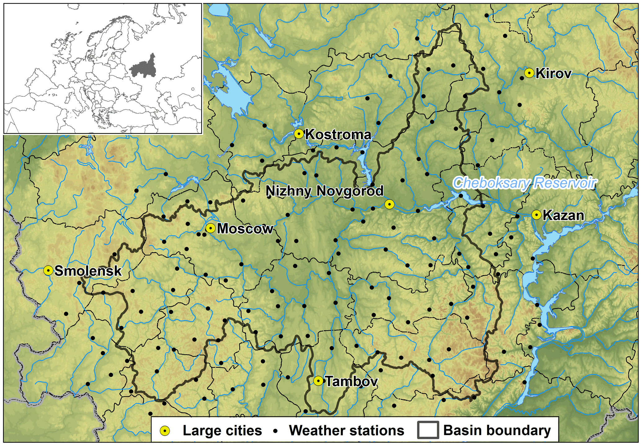
The Cheboksary Reservoir is located on the Volga River in the central part of the European part of Russia. It was constructed in 1982 to become the 11th member of Volga-Kama reservoir cascade, with Nizhegorodskoe reservoir upstream and Kujbysevskoe reservoir downstream of it. The total unregulated basin area of the Cheboksary Reservoir is 373 800 km2 (Fig. 1). Its main tributaries – Oka, Sura and Vetluga rivers – account for 80 to 90 % of annual inflow into the reservoir.
Local climate conditions can be described as moderately continental, with a cool snow-abundant winter and a relatively hot summer. Mean annual temperature ranges from 1.4 ∘C in the northern part of the basin to 4.8 ∘C in the southern part. During wintertime air temperature may fall as low as −35– −40 ∘C. The annual precipitation amount ranges between 650 and 750 mm throughout the territory. Around 60 % of the precipitation occurs as rain. Most winter precipitation is stored as snow cover, emerging in mid-December and lasting until mid-April. Snow water equivalent ranges from 50 mm in the south-western part up to 100–120 mm in the north. Springtime snowmelt contributes to the high-flow freshet – the dominating hydrological season accounting for around 65% of the total annual inflow into the reservoir (51.3 km3). Typically, the freshet commences around mid-April and lasts until June. The mean volume of inflow for the period of reservoir operation (1982–2016) is 33.4 km3, and the mean maximum inflow discharge is 9355 m3 s−1.
3.1 Operational data-driven forecast of spring inflow into the Cheboksary Reservoir: current practice
The methodology for forecasting the spring inflow into the Cheboksary Reservoir was developed by Chemerenko (1992) on the basis of the so-called physical–statistical approach, originally proposed for the reservoirs of Middle Volga in the mid-1960s (Zmieva, 1964; Gelfan and Motovilov, 2009). This approach is currently in use by the Russian hydrometeorological service (Roshydromet) for inflow forecasting into all reservoirs located on the Middle Volga River.
Water inflow volume Y into the Cheboksary Reservoir is forecasted according to the following linear equation:
where yi is the runoff forecast at streamflow gauge i, located on the reservoir tributaries, as follows: i = 1 – Oka River, Polovskoe gauge (drainage area F = 99 000 km2); i = 2 – Klyazma River, Kovrov gauge (F = 24 900 km2); i = 3 – Vetluga River, Vetluzhsky gauge (F = 27 400 km2); i = 4 – Sura River, Poretsky gauge (F = 50 100 km2); i = 5 – Tsna River, Knyazhevo gauge (F = 13 600 km2). αi and β are the regression coefficients estimated from the streamflow data observed at the corresponding gauge.
The runoff volume yi at the ith gauge is forecasted by a unified procedure. The predictors are basin-averaged snow water equivalent (S, mm), soil freezing depth, (FD, cm), soil moisture index (W, dimensionless) on a forecast issue date and total precipitation (x, mm) during the forecast horizon.
Runoff volume at each gauge is calculated as follows:
where S1 and S2 are the snow water equivalent at the forecast issue date within the deep frozen (FD ≥ 60 cm) and non-deep frozen (FD < 60 cm) parts of the river basin, respectively, derived from snow observations; x is the total precipitation for the forecast horizon, assigned as the climatic mean; f is the fraction of the basin area covered by deep-frozen soil, derived from soil freezing observations; θ is the soil moisture index, calculated from the precipitation amount during the preceding autumn period; η is the runoff coefficient from the basin fraction with non-deep frozen soil calculated as a function of θ; a, b, c, θmin are the parameters derived from hindcasts for the 30-year period before the reservoir filling in 1982.
The operational forecast of water inflow volume into the Cheboksary Reservoir for April–June period is issued just before the beginning of this period (27 March) and then updated 2–3 times during April–May. In this paper, the operational deterministic forecast (not updated, i.e. issued before the beginning of April) is compared with the deterministic forecast derived from the model-based ensemble-mean forecast described below (see Sect. 3.2.2).
3.2 Model-based ensemble forecast technique and verification measures
3.2.1 Modelling tools
Hydrological model
The ECOMAG (ECOlogical Model for Applied Geophysics) is a semi-distributed process-based hydrological model describing snow accumulation and melt, soil freezing and thawing, water infiltration into unfrozen and frozen soil, evapotranspiration, the thermal and water regime of soil and the overland, subsurface and channel flow with a daily time step (Motovilov et al., 1999). The model accounts for measurable watershed characteristics such as surface elevation, slope, aspect, land cover and land use, soil and vegetation properties. The parameters are spatially distributed by partitioning the watershed into sub-basins (elementary basins). Parameterization of the sub-grid processes is described by Motovilov (2016). The model is driven by time series of daily air temperature, air humidity and precipitation intensity.
The model was applied at an earlier time for hydrological simulations in many river basins with highly varying sizes and characteristics – from small- to medium-sized European basins (Gottschalk et al., 2001) to the large Volga, Lena and Mackenzie basins with watershed areas exceeding 1 million km2 (Motovilov 2016; Gelfan et al., 2017).
In this study, a digital elevation model with 1 km × 1 km spatial resolution was used for the basin discretization and river network construction. A total of 1045 elementary basins were delineated, with an average area of 340 km2. The model forcing data for each elementary basin were interpolated from the 157 weather stations' data (see Fig. 1), employing the inverse distance method. Most parameters are physically meaningful and were derived through available measurements of the basin characteristics (topography, soil and vegetation properties).
The model was calibrated and validated against the Cheboksary Reservoir daily water inflow observations beginning from 1 January 1982 (the first year after the reservoir was filled to capacity) to 31 December 2016: the calibration covered the period of 2000–2010; the rest of the data were used for the model evaluation. The ECOMAG calibration procedure is described in detail by Gelfan et al. (2015). It is worth emphasizing two specific aspects concerning this procedure. First, the values of several key parameters pre-assigned from literature or from the available measurements are considered as the initial approximations of the optimal values, and the latter are sought within the neighbourhood of the initial, pre-assigned values. Second, during the calibration process, the ratios between the initial values of the distributed parameter corresponding to different soils, landscapes and vegetation are preserved. This approach allows for the integration of important hydrological knowledge into the optimization procedure. The Nash and Sutcliffe (1970) efficiency criterion NSE is adopted to represent the goodness of fit of the simulated and measured variables.
Multi-site weather generator (MSFR_WG)
The Multi-Site FRagment-based stochastic Weather Generator (MSFR_WG) is a stochastic model that uses a Monte Carlo simulation to generate time series of daily weather variables (precipitation, air temperature and air humidity deficit), retaining statistical properties, both spatial and temporal, of the corresponding observed variables. This modelling procedure is based on the so-called “spatial fragments' (SFR) resampling method” initially presented by Gelfan et al. (2015). The SFR method is a modification of the temporal fragments' (TFR) method proposed by Svanidze (1980) for the stochastic simulation of highly autocorrelated time series.
The SFR resampling method includes the following steps.
-
N normalized fields (spatial fragments, SFRs) of weather variables are computed on the basis of the available meteorological data. SFRs are computed for each of N years of observations by dividing each daily value of the specific variable by the corresponding spatially averaged annual value.
-
Monte Carlo simulation of the synthetic time series of M spatially averaged annual weather variables, reproducing temporal statistical features of the corresponding annual variables derived from observation data, is conducted. Cross-correlation between annual values of the simulated weather variables is taken into account through the Cholesky's decomposition method (see e.g. Press et al., 2007).
-
The synthetic daily fields of weather variables are calculated by multiplying the computed SFRs (see step 1) by the Monte Carlo-simulated spatially averaged annual value of the corresponding variables (see step 2). SRFs are randomly chosen from the available set by the Latin hypercube method (McKay et al., 1979).
The advantage of MSFR_WG is that it has a small number of free parameters in comparison with the widely used multi-site weather generators (see e.g. Khalili et al., 2011 and references therein), and it does not require complex estimation procedures. Such features typically indicate that the model has high robustness.
3.2.2 Ensemble forecasting technique
The proposed ensemble forecasting procedure utilized in this study was verified by producing hindcasts of water inflow into the Cheboksary Reservoir from 1 April for 3 months ahead (up to 30 June). The hindcasts cover a 35-year period between 1982 and 2016. (Hereafter, we use the term “forecasts” for these hindcasts.) For each ith year of the verification period (i = 1, 2, …, 35), the procedure consists of the following steps:
-
Spin-up of ECOMAG-based simulations (“warm start”) is conducted using meteorological observations data prior to the forecast issue date (31 March) in order to calculate the initial watershed hydrological state (soil, snow and channel water contents, groundwater level, soil freezing depth, etc.) that initializes the forecast. The simulations start from the end of the previous freshet, i.e. 8–9 months before the forecast issue date.
-
A weather scenario1 is selected from the NESP-member ensemble of the observed weather or from the NWG-member ensemble of the generated weather for the forecast horizon (NESP = 51; NWG = 1000; see Sect. 4.3.1).
-
The daily inflow hydrograph is simulated by the ECOMAG model driven by the selected scenario.
-
The next weather scenario (step 2) is repeatedly selected from the ensemble and calculation of the corresponding inflow hydrograph (step 3). The corresponding ensemble of N inflow hydrographs is formed (N = NESP or N = NWG).
-
From each of the modelled hydrographs, the following inflow characteristics are derived: (1) inflow volume (hereafter referred to as W), (2) maximum inflow discharge (Qmax), (3) number of days with the inflow discharge above the mean observed discharge for the forecast horizon (Nq) and (4) number of days with the inflow discharge above the mean maximum observed discharge for the forecast horizon ().
-
Deterministic (ensemble mean) and probabilistic forecasts are derived and verified for each of the inflow characteristics.
3.2.3 Verification measures
To verify deterministic and probabilistic model-based forecasts, as well as to compare them with each other and with the operational data-driven forecast of water inflow into the Cheboksary Reservoir, we used the following, quite traditional, measures of the forecasts' efficiency and skill.
For the deterministic forecast verification, the mean error, relative bias, root-mean-squared error (RMSE) and Pearson's correlation coefficient r were used. In addition, for presentation, we used a Taylor diagram (Taylor, 2001), which combines three forecast characteristics in one chart, namely the forecast standard deviation, the RMSE and the correlation coefficient between the observations and the forecasted values.
For categorical forecast verification, we used measures that can be calculated from a contingency table (Ferro and Stephenson, 2011), such as the probability of detection (POD, which shows the correct forecast fraction of the observed events), the false alarm ratio (FAR, which shows the fraction of forecasts that did not occur), the frequency bias (which shows correspondence of the observed and the forecasted events), the Heidke skill score (HSS, which shows the advantage of the forecast as compared to a random forecast), the Hansen and Kuipers score (KSS, which can detect if the forecast is hedging) and the Symmetric Extremal Dependency Index (SEDI, which evaluates the performance of the forecast of rare binary events).
The probabilistic ensemble forecasts' performance was assessed by several verification measures. The ability of forecasts to correctly predict the category of events that occurred within several categories was measured by the ranked probability score (RPS) (Wilks, 1995), which can also be treated as the mean squared error of the probabilistic forecast. The probability forecast efficiency relating to streamflow climatology was measured by the ranked probability skill score (Wilks, 1995). To visualize the specifics of probabilistic forecasts, three diagrams were employed. A predictive Q–Q (quantile–quantile) plot (Laio and Tamea, 2007) was used to assess the degree of correspondence between the cumulative distribution function of predictions and the observed values. A reliability diagram (Hartmann et al., 2002) was used to plot the forecast probability against the relative frequency of the observations in the corresponding forecast probability bin. Finally, the discrimination diagram (Wilks, 1995) was used to show the frequency of each forecast probability for events and non-events.
A full list of the aforementioned verification measures and their formulations, units and value ranges are presented in Table S1 (Supplement).
4.1 Calibration and evaluation of the hydrological model
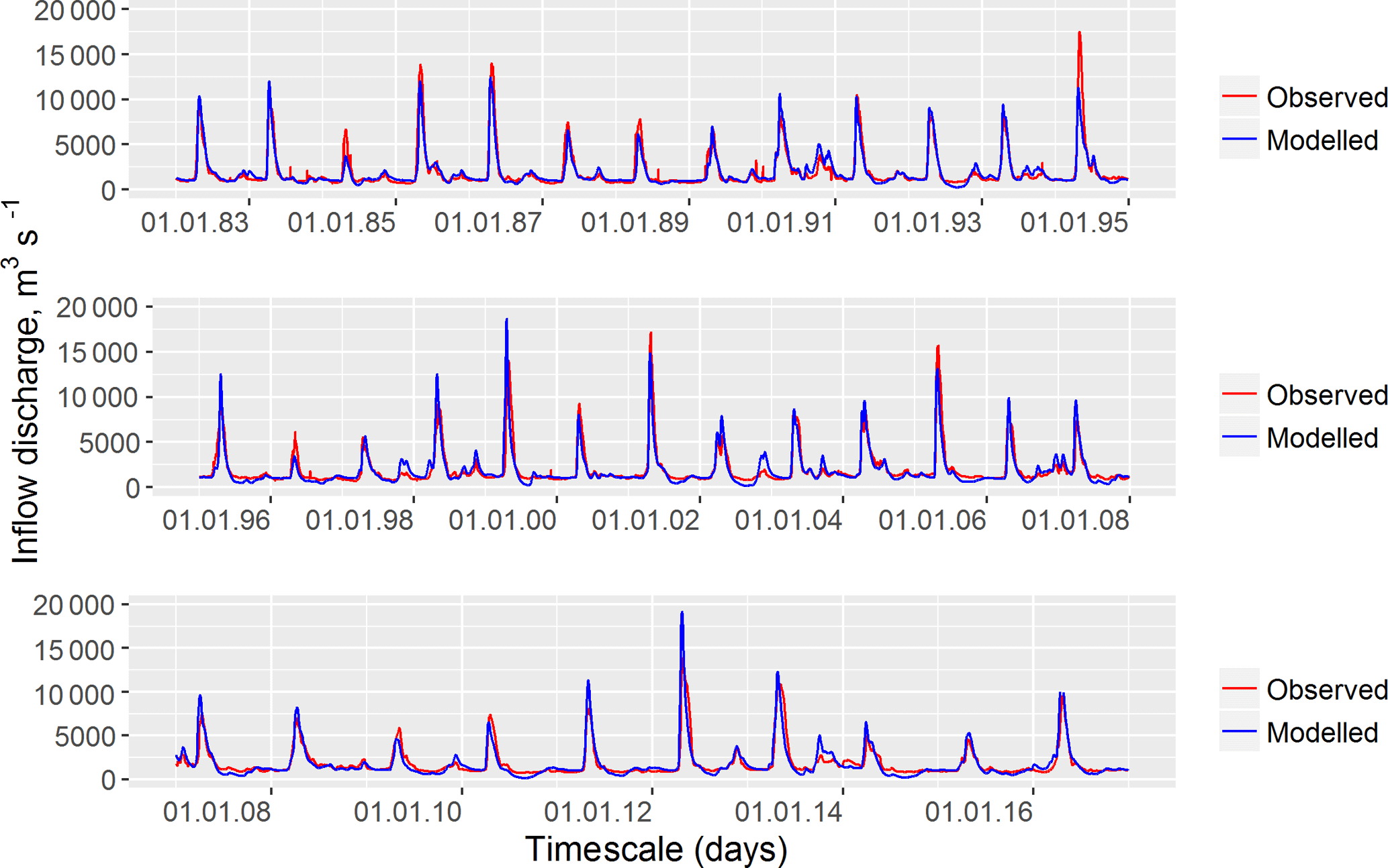
The hydrological model was calibrated and evaluated against the daily time series of water inflow into the Cheboksary Reservoir for the periods of 2000–2010, 1982–1999 and 2011–2016. The observed inflow data do not account for inflow from the upstream Nizhegorodskoe reservoir. Figure 2 compares hydrographs of the observed and the simulated daily inflow discharges. The Nash–Sutcliffe efficiency for daily inflow discharge is rather high (NSE = 0.80) and ranges from 0.79 for the evaluation period to 0.83 for the calibration. One can see that the model demonstrates good performance with respect to this criterion. Additionally, a small difference between the criteria estimated for the calibration and evaluation periods confirms the model robustness (Gelfan et al., 2015).
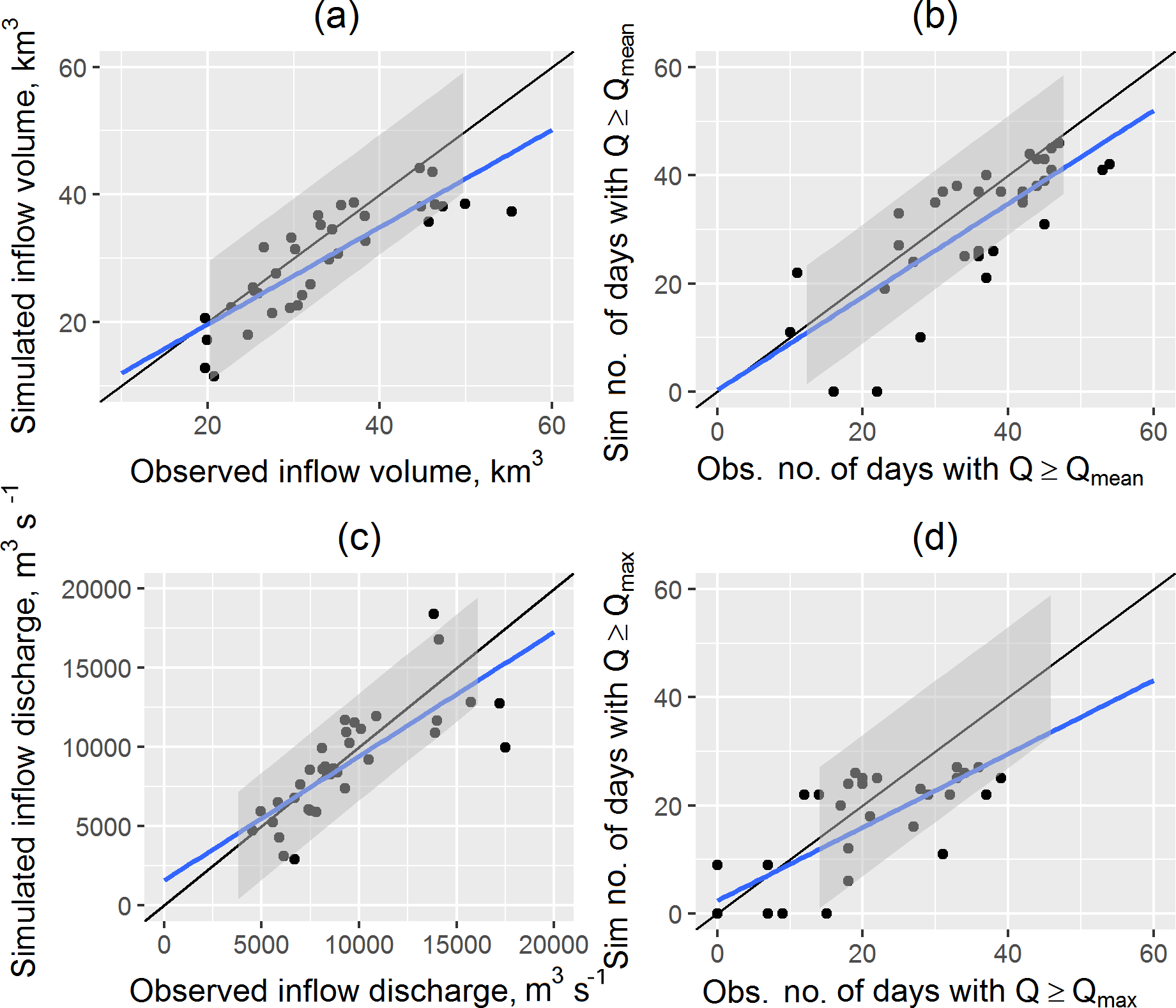
Figure 3Scatterplots for the observed and simulated characteristics of inflow into the Cheboksary Reservoir during April–June: volume W (a), the number of days above the mean inflow discharge Nq (b), the maximum discharge Qmax (c) and the number of days above the mean maximum inflow discharge (d). The blue line represents the linear fit. The black line represents the perfect fit. The grey shaded area denotes the variance band of ±1 SD (standard deviation) of the respective observed values.
The model performance was also tested by comparison of the observed and simulated inflow characteristics, which were then used for the forecast verification and are listed in Sect. 3.2.2. Figure 3 shows scatterplots of the observed and simulated characteristics of the inflow into the Cheboksary Reservoir in April–June. In general, the inflow volume is well simulated, yet slightly underestimated for the high flows (above 50 km3; see Fig. 3a). Maximum inflow discharge is a highly uncertain characteristic but is still well simulated by the model (Fig. 3c). The number of days above a certain inflow discharge threshold is a highly important characteristic for various uses, e.g. waterways' navigation and water supply. For the number of days above long-term (1982–2016) mean inflow discharge during the period between April and June, the model shows fewer days than the observed ones (Fig. 3b) – 31 compared to 36 days, on average for the whole period. For the number of days above long-term mean maximum inflow discharge the model also shows fewer days (Fig. 3d) – 13 compared to 17 days, on average.
The relative bias of the inflow volume in April–June for the whole period 1982–2016 is −3 %; the RMSE of the inflow volume (5.23 km3) is 55 % of the observed data standard deviation (σW = 9.41 km3). The relative bias of the maximum inflow discharge is 5 % m3 s−1; the RMSE is 2321 m3 s−1, that is 30 % lower than the standard deviation of the observed maximum inflow discharge (3385 m3 s−1).
The obtained results allow us to conclude that the developed model can be considered as a suitable tool for the long-term hydrological forecasting of spring water inflow into the Cheboksary Reservoir.
4.2 MSFR_WG: parameter estimation and model testing
Time series of daily precipitation, air temperature and humidity deficit observed at the meteorological stations located at the Cheboksary Reservoir basin for 51 years (1966–2016) are used to estimate the nine parameters of the developed stochastic model. The parameters estimated by the method of moments are shown in Table S2. The stochastic models were comprehensively tested for their ability to reproduce the main statistical characteristics of meteorological processes at the Cheboksary Reservoir basin. For testing, we only compared those characteristics of the observed and simulated time series, which are neither the parameters of the model, nor a single-valued function of the parameters as suggested in Gelfan (2010). Statistics of the 1000-member Monte Carlo-generated ensemble of the daily meteorological variables were compared with the following corresponding statistics derived from observations: mean and variation of annual and monthly values and autocorrelation functions of daily and monthly values of the specific variables. Results demonstrating comparison between statistical properties of the observed and simulated series are shown in the Supplement for spring months and for several selected stations (Figs. S1S–S8).
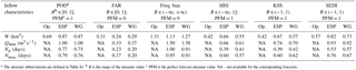
Table 1Statistics of the operational (Op.) and the ensemble (ESP and WG) deterministic forecasts of inflow into the Cheboksary Reservoir for April–June in 1982–2016.
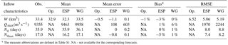
* The measure abbreviations are defined in Table S1. NA – not available for the corresponding forecasts.
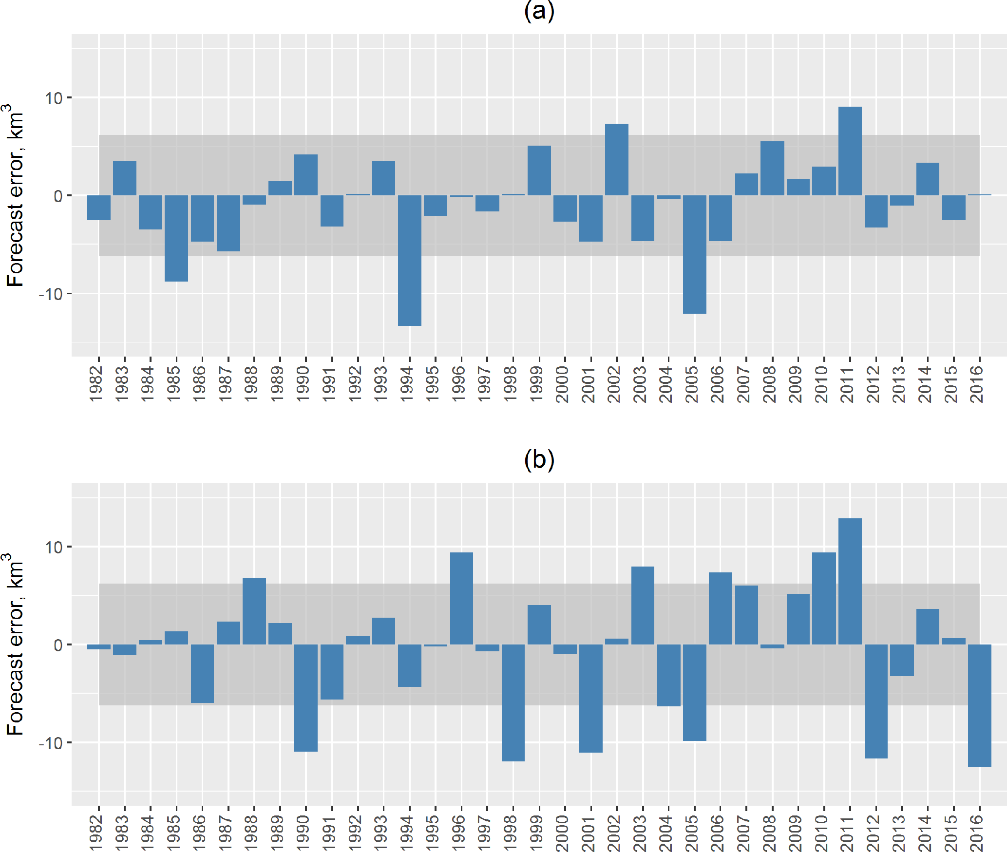
Figure 4Errors of the ESP-based (a) and operational (b) forecasts of the April–June volume of water inflow into the Cheboksary Reservoir. (Solid lines present boundaries of the acceptable error, which equalled ±0.674σW, where σW = 9.61 km3 is the standard deviation of the observed inflow volume.)
Figures S1 and S8 demonstrate the ability of the developed weather generator to reproduce annual and monthly mean values of air temperature, precipitation and humidity deficit. Figure S8 demonstrates good correspondence between the distributions of the observed and modelled precipitation, as well as Fig. S2, in which a good match between the observed and the modelled coefficient of variation can be seen. Despite some bias, the model errors do not appear to be systematic. The ability of the generator to preserve the spatial structure of the weather variables was examined by evaluating the spatial correlation curves (Fig. S7) for temperature and precipitation, which demonstrate a close match for both daily temperature and precipitation.
4.3 Forecast verification
4.3.1 Ensemble (model-based) and operational (data-driven) deterministic forecasts
We verified the two types of the ensemble forecasts (ESP-based and WG-based) and compared them with each other and with the operational forecasts of water inflow into the Cheboksary Reservoir for April–June 1982–2016. To make a deterministic forecast, the forecasted inflow characteristics were averaged over the corresponding ensembles (51-member in the case of the ESP-based forecast and 1000-member for the WG-based forecast) to produce a single-value forecast of the desired characteristic: W, Qmax, Nq, . Operational forecasts of inflow volume for the same April–June periods of 1982–2016 were obtained from official Roshydromet forecast bulletins (reports). All forecasts were analysed to assess the forecast performance measures: the mean absolute error, the bias and the RMSE. The results are presented in Table 1.
First, the deterministic forecasts of the inflow in April–June were compared to the operational forecasts for 1982–2016. As shown in Table 1, the mean error of the operational forecasts appears to be quite low (around 1 %) and close to those of the ESP and WG ensemble average values. However, the operational forecasts' RMSE values are significantly higher than those of the ESP and WG forecasts and account for almost 70 % of the observed inflow volume variability σW = 9.61 km3. For the ESP- and WG-based forecasts these values are around half of σW.
Figure 4 compares the inflow volume forecast errors of the operational forecasts (Fig. 4a) with the ESP-based forecast errors (Fig. 4b). The shaded area in the figures represents the area of the acceptable error [−0.674σW; 0.674σW] = [−6.48; 6.48 km3]. In Russian operational forecasting practice, a forecast is considered acceptable if its error falls into this area, and the forecast acceptability is calculated as the ratio of the acceptable forecasts to the whole number of forecasts. According to the assumption of the Gaussian distribution of the forecast errors, 50 % of the forecasts by climatology should fall into this interval. It can be seen from Fig. 4 that 5 of the 35 ESP-based forecasts (in 1985, 1994, 2002, 2005 and 2011) and every third (12 of 35) operational forecasts were not acceptable; i.e. the ESP-based forecast acceptability is 89 % and that of the operational forecast is 66 %. Note that the unacceptable forecasts in both cases occurred in the years when the spring precipitation amount was notably different from the corresponding climatic mean.

Figure 5Normalized Taylor diagram of ESP-based (in blue) and WG-based (in red) forecasts of the inflow volume W (circles), the maximum inflow discharge Qmax (triangles), the number of days with the inflow discharge above the mean Nq (squares) and the number of days with the inflow discharge above the maximum (diamonds).
To compare the ESP-based and the WG-based forecasts, we present them in the form of a Taylor diagram (Fig. 5; Taylor, 2001), which combines three forecast characteristics in one chart, namely, the forecast standard deviation, RMSE and the correlation coefficient between the observed and the forecasted values of the inflow characteristics. The values of all characteristics are normalized by dividing the RMSE by the standard deviation of the observations. This normalization provides a demonstration of the forecast efficiency expressed in fractions of the observed standard deviation. As long as the forecast RMSE is less than the standard deviation of the observations, the forecast can be considered efficient against climatology.
It can be seen from Fig. 5 that the ESP-based forecasts of W, Qmax and are slightly better correlated with the observations than the WG-based forecasts. Pearson's r values of the ESP-based forecasts are over 0.8 for all characteristics, except for Nq. Forecasts of Nq are less correlated with the observations, with r values for ESP-based and WG-based forecasts equal to 0.73 and 0.63, respectively. Forecasts of Qmax and show normalized RMSE values around 58–67 % of the standard deviation of the corresponding observed characteristics.
Table 2Verification measures for the binary forecasts (Cheboksary Reservoir, April–June of 1982–2016).
a The measure abbreviations are defined in Table S1. b R is the range of the measure value. c PFM is the perfect forecast measure value. NA – not available for the corresponding forecasts.
For the purpose of reservoir management, it is often crucial to determine whether the expected inflow characteristic will exceed the corresponding mean value. To verify the methodology's capability of predicting this exceedance, the observations and forecasts were converted into binary vectors, with a value of 0 representing the event of non-exceedance of the mean annual value and a value of 1 representing the event occurrence. For example, for W, the event occurs with the exceedance of mean inflow volume during April–June. The forecast binary measures assessed with the use of the contingency tables and described in Table S1 are shown in Table 2.
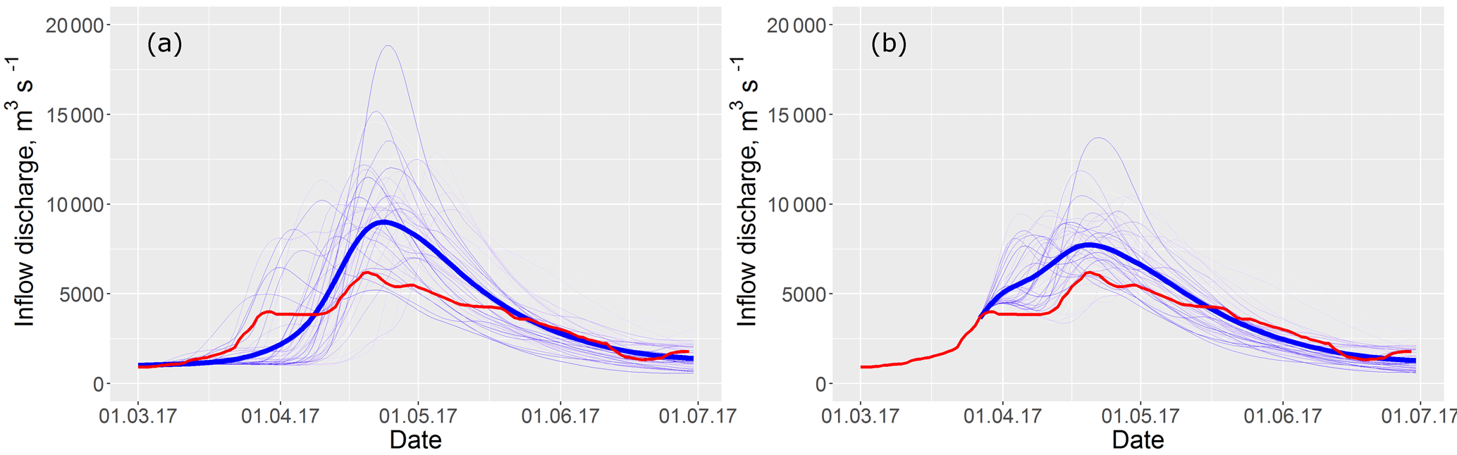
Figure 6The ESP-based forecast of daily inflow discharge for the period from 1 April till 30 June 2017 issued on 1 March (a) and 27 March (b). The thin blue lines represent the ensemble of the forecasted hydrographs, the bold blue line represents the mean ensemble hydrograph and the red line represents the observed hydrograph of inflow into the Cheboksary Reservoir.
The forecasts show good detection estimates (even perfect for Qmax) for both model-based methodologies. However, as the frequency bias is high, this might be the result of overprediction, as with the high values of the FAR and KSS. For W and Qmax, the forecast accuracy with a HSS of around 60 % is better than the accuracy of random chance; this means that the forecast is capable of detecting the occurrence of rare extreme events, which is shown by high values of the SEDI. Overall, the presented binary verification measures demonstrate a slight advantage of the ESP-based forecasts over the WG-based forecasts, though the differences are not substantial.
Binary measures of the operational forecasts of inflow volume are worse than those of the model-based forecasts. For instance, only 69 % of the observed events (exceedance of mean inflow volume) are correctly forecasted by the current operational methodology, and its accuracy relative to that of random chance is less then 50 %. The ability of a user to detect rare events on the basis of the operational forecast is also much lower than with the help of ensemble forecasts.
Thus, both continuous (Table 1) and binary (Table 2) model-based forecasts of inflow volume appear to be more preferable, in general, than the corresponding operational forecasts. However, as one can see from Fig. 4, there were several years when the operational forecasts were more accurate (in terms of the absolute error) than the ensemble ones. We found that most often the operational forecast outperforms the model-based forecast in those years when the modelled initial snow water equivalent (SWE) on the forecast issue date notably differed from the observed SWE. Since the latter is the main factor affecting the freshet volume, more accurate (observed) initial snow conditions used in Eq. (2) resulted in a more accurate forecast than the one initiated from the simulated SWE.
4.3.2 Freshet of 2017: testing the ensemble methodology
In the beginning of spring 2017, the basin's pre-melt conditions were close to climatology: snow water storage was 10 to 15 % above the long-term mean value, and soil water content and freezing depth were close to the corresponding mean values. However, the weather conditions during the spring freshet formation appeared to be significantly different from climatology. Anomalous warm and sunny weather that settled over the basin in the first half of March led to the commencement of snowmelt and river stage ascent at least half a month earlier than the mean dates. The last decade of months of March was, on the contrary, cold and damp, and the precipitation amount was twice above normal for this period. As a result, by the end of March the inflow volume (5.13 km3) into the reservoir exceeded mean March inflow by 32 %. Periods of intense snowmelt interchanged with cold spells and a large amount of precipitation, including snowfall during April and May 2017 (a number of stations even registered snowfall in June). Such diversity in weather conditions during the snowmelt period and their difference from the climatology resulted in a rather untypical regime of inflow into the Cheboksary Reservoir.
The ESP-based forecasting technique was tested in operational mode during the freshet period of 2017. The forecasts were issued on 1, 15 and 27 March for the period from 1 April till 30 June. Figure 6 shows daily forecast ensembles for this period compared to the observed inflow data.
Figure 6 shows the outcome of the anomalous weather conditions that led to an earlier increase of the inflow in mid-March (see Fig. 6a), which was not captured by the mean ensemble hydrograph of the forecast issued on 1 March. However, several scenarios of the ensemble show the behaviour of inflow to be similar to that observed. The forecast issued on 27 March showed the ongoing increase in inflow discharge; however the colder weather conditions led to inflow stabilization, not captured by the forecast. One can see visible improvement of the mean ensemble hydrograph issued on 27 March (Fig. 6b) compared with the one issued on 1 March (Fig. 6a).
Box plots of the ESP-based forecasts of different inflow characteristics are presented in Fig. 7. All forecasts of inflow volume showed low errors (Fig. 7a), unlike the maximum discharge forecasts (Fig. 7b); however, the Qmax forecast range envelops the observed maximum inflow discharge. Both forecasts of number of days over thresholds showed low errors (Fig. 7b and d); e.g. just before the beginning of April we correctly forecasted a low freshet with the absence of days when inflow discharge exceeds the mean maximum discharge for the period of observations.
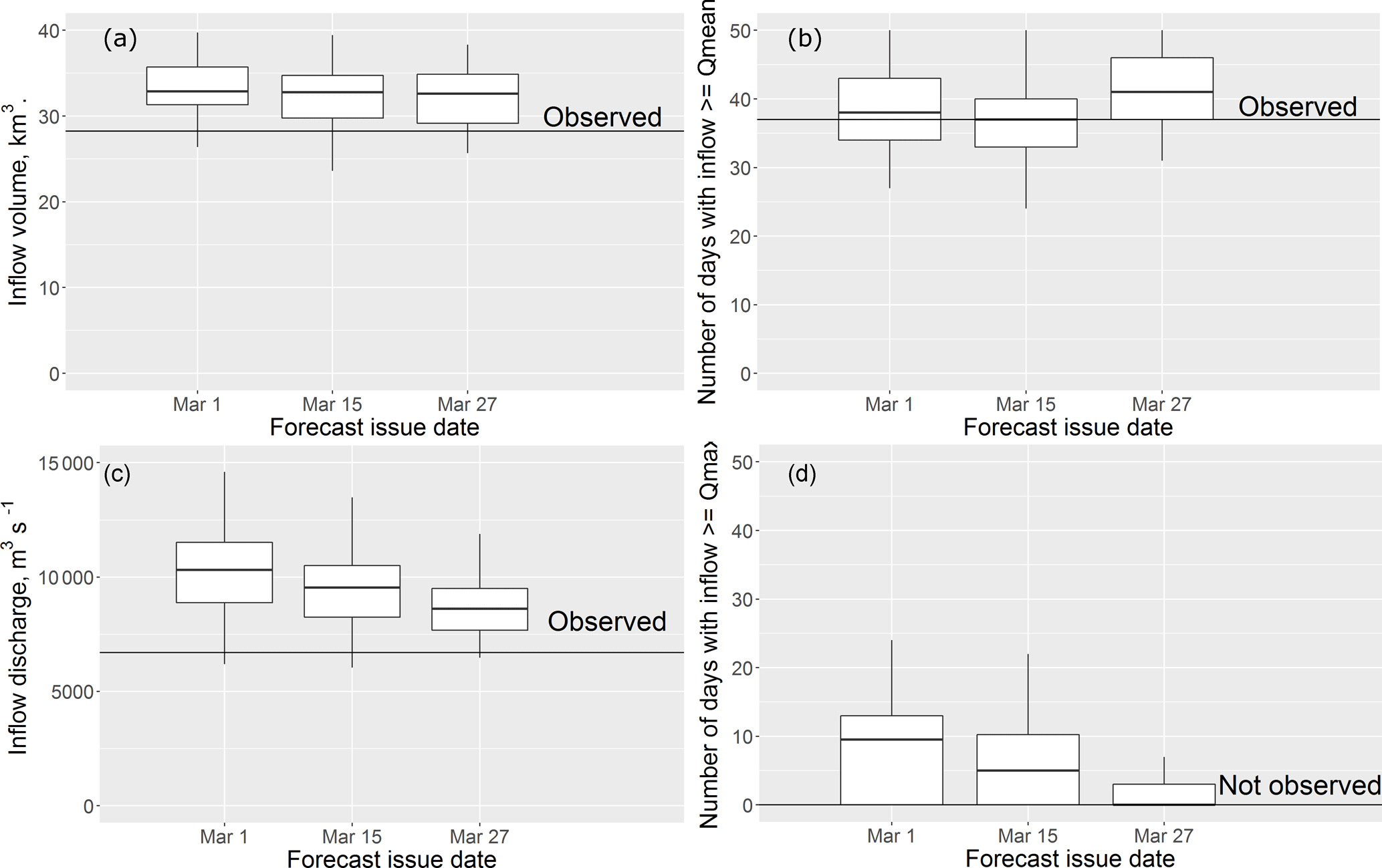
Figure 7Box plots of the ESP-based forecast of the inflow volume (a), the number of days with the inflow discharge above the mean observed discharge (b), the maximum inflow discharge (c) and the number of days with inflow discharge above the mean maximum observed discharge (d) for the period from 1 April till 30 June 2017. The solid horizontal line shows the observed value of the corresponding characteristic.
In 2017, Roshydromet also issued a forecast of spring water inflow into the Cheboksary Reservoir on the basis of the methodology presented above (Fig. 8). In contrast with the results presented in Table 1 and Fig. 4, which demonstrate the general advantage of the ESP-based forecasts over the operational forecasts for 1982–2016, in 2017, the operational forecast of the inflow volume appears to be better. A possible explanation is again found in the simulation errors of the pre-melt SWE used as initial conditions for the ESP-based forecast.
4.3.3 Probabilistic forecast
In this section, the operational forecast, which is issued in deterministic form only, is not discussed.
One of the main advantages of ensemble forecasting is the ability to assess the uncertainty that is nested in the future possible behaviour of the hydrological system. The resulting ensemble is used to create cumulative distribution functions (CDFs) of the desired characteristic in jth forecast as
where M refers to the forecast probability bins on the interval [0; 1], N is the total number of forecasts and fi is the probability of forecast in mth bin.
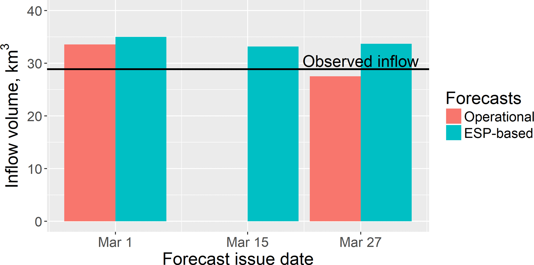
Figure 8The ESP-based and operational forecasts of volume of water inflow into the Cheboksary Reservoir for the period from 1 April till 30 June 2017 (the line indicates the observed value).
Table 3Ranked probability score and skill score for the forecasts.
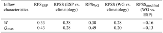
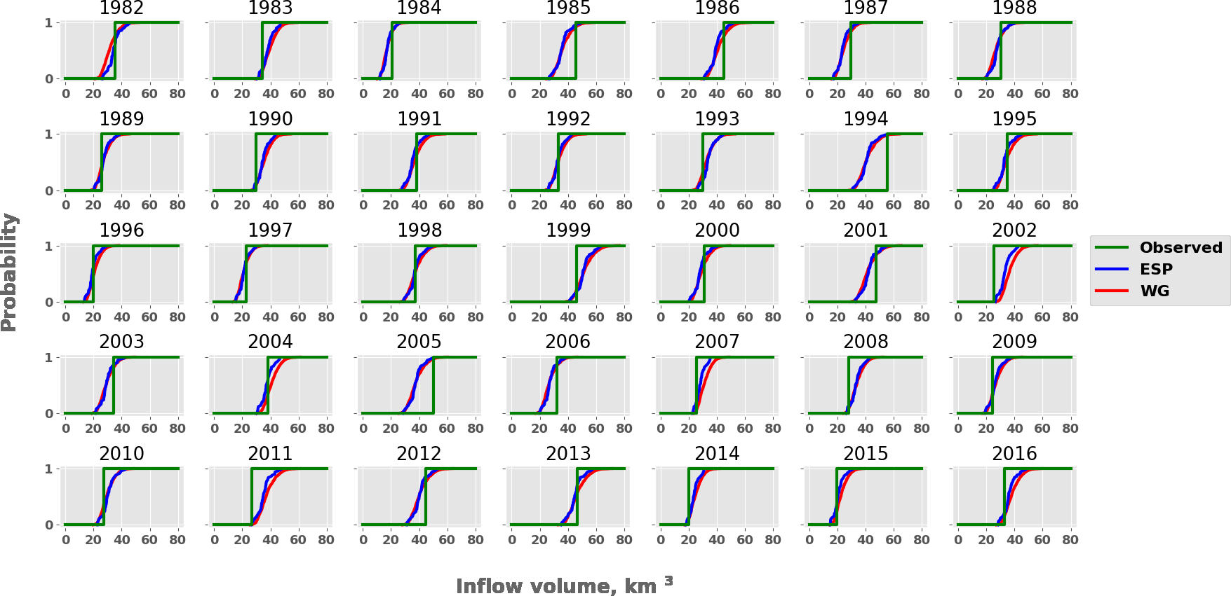
Figure 9Cumulative probability distribution functions for W in April–June for all years between 1982 and 2016. The green line represents the observed inflow, the blue line represents the ESP-based forecast and the red line represents the WG-based forecast.
CDFs of the forecasted inflow volume W for the period from 1 April to 30 June of 35 years (1982–2016) are shown in Fig. 9. Three CDFs are combined in each plot: two CDFs of forecasts calculated under ESP-based and WG-based weather scenarios and the CDF of the observed inflow volume in the specific year (CDFs of observations can be represented as the Heaviside step function). One can see from Fig. 9 that for most of the years, the inflow is not far from the most probable one; in other words, the CDF of the forecasts crosses the CDF of observations at around 50 % probability. For almost all years observed inflow lies within the range of the ensemble. Exceptions are 1994, 2002, 2005 and 2011; i.e. once every 8–9 years, on average, the ensemble forecast range does not cover the observed inflow because of large forecast errors.
To quantify the ability of forecasts to predict the probability of an event occurring within the pre-assigned inflow categories, we used the RPS measure. The forecast efficiency was measured by the RPSS criterion, relating the verified forecast to streamflow climatology (both RPS and RPSS formulations are presented in Table S1).
Both forecasts demonstrate a moderate improvement over climatology: according to the RPSS value, around 30 % on average both for W and for Qmax (Table 3). Probably, accounting for a seasonal weather forecast and conditioning historical weather patterns on this forecast could result in a greater improvement over the streamflow climatology; however a reliable seasonal weather forecast for the study region is not available.
In addition, we compared the ESP-based and the WG-based forecasts by setting the former one as a reference forecast. The modified RPSS is formulated in this case as
As one might expect from a comparison of the unmodified RPSS measures, the modified one showed that the WG forecasts are less skilful than the ESP, with modified RPSS values of −0.16 for W and −0.13 for Qmax.
To compare quantiles of the forecasted characteristics with the quantiles of the corresponding observations, we used the predictive Q–Q plot (Laio and Tamea, 2007). As one can see from Fig. 10a, the predictive Q–Q plot of the inflow volume forecasts demonstrates good agreement with the distribution of the observations. This is fairly consistent for both methodologies and for all quantiles, but for rare events there is an underestimation of the predictive uncertainty, expressed as an offset from the 1 : 1 line in the upper right corner of the plot. For the maximum inflow discharge (Fig. 10b), one can see overprediction in both methodologies. However, the behaviour of ESP-based and WG-based forecasts of rare events is different in terms of predictive uncertainty. In particular, the WG-based forecasts of the events of low exceedance probability appear to be closer to the 1 : 1 line.
Additionally, comparisons between the ensemble forecasts of both types can be made based on the reliability and discrimination diagrams presented in Figs. S9–S12.
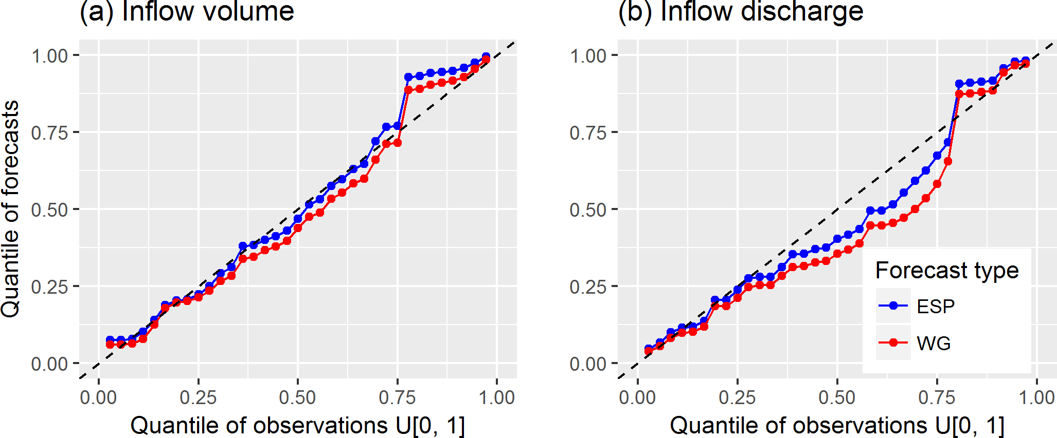
Figure 10Predictive quantile–quantile plots for inflow volume (a) and inflow discharge (b) forecasts.
Overall, all presented measures of the probabilistic forecast performance are slightly better for the ESP-based forecasts than for the WG-based forecasts, though the differences are not significant and hardly interpretable. At the same time, verification measures obtained from the large ensemble of the WG-based forecasts are expected to be more statistically reliable, which is demonstrated in the next section for the two measures, CDF and RPSS.
4.3.4 Ensemble size effect on the verification measures: two examples
It can be seen from Fig. 9 that the CDFs appear to be close to each other for both ensemble methodologies used. However, the sample variance of the CDF is significantly different due to a different number of scenarios in the ensembles: 51 in the ESP-based ensemble compared to 1000 in the WG-based ensemble. To illustrate this difference, we assessed confidence bands for CDFs derived from both forecasting approaches. Two-sided confidence bands were expressed through the Dvoretzky–Kiefer–Wolfowitz inequality as (e.g. Massart, 1990)
where F(x) and are the CDF's ordinate and its empirical estimation from a sample of size n, respectively; ε is the constant depending on the significance level α as
For the pre-assigned confidence probability p = (1 − α), the upper (U(x)) and the lower (L(x)) confidence bands of the empirical CDF are defined from Eqs. (5) and (6) as
Figure 11 demonstrates the difference between 95 % confidence intervals of the ESP-based inflow volume forecast as compared to the corresponding intervals of the WG-based forecast. We believe that the presence of the mentioned difference should be taken into account by the ensemble forecast developers when they use statistical verification measures for the assessment of forecast performance, as well as by the users when they interpret the forecasts.

Figure 11Cumulative probability distribution functions for W in April–June for selected years between 1982 and 2016 for the ESP-based forecast (a–c) and the WG-based forecast (d–f). The shaded area presents the interval of 95 % confidence probability.
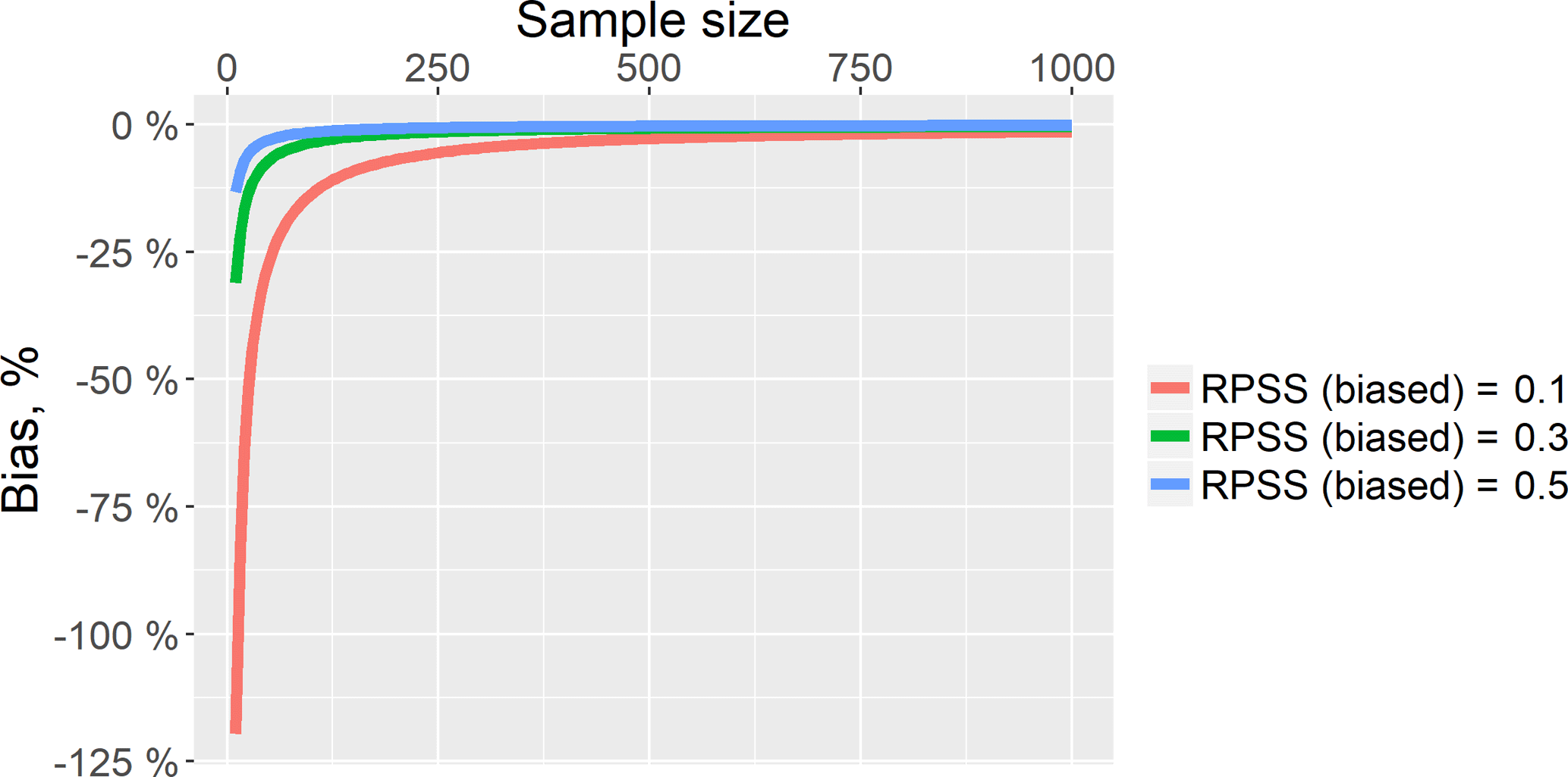
Figure 12Negative bias of the RPSS estimate in dependence on the ensemble size and the RPSS value.
One can conclude from Table 3 that the RPSS criterion demonstrates the advantage of the ESP-based probabilistic forecast over the WG-based one as compared to climatology. However, it is important to take into account that the RPSS measure is strongly dependent on ensemble size and negatively biased (see, for instance, Müller et al., 2005; Weigel et al., 2007). A de-biased estimate of the RPSS can be formulated as by Weigel et al. (2007):
where D is the correction term depending on the ensemble size, the climatological probabilities and the number of categories. For a very large ensemble size, the correction term D converges toward zero and the RPSSD converges towards the RPSS.
Figure 12 demonstrates the dependence of the RPSS bias on sample size built with the use of the approximation of D presented in Weigel et al. (2007).
One can see from this Fig. 12 that using the 51-member ensemble (i.e. the ESP-based ensemble), the bias can reach tens of percent depending on the RPSS estimate. Using the 1000-member ensemble, the bias is close to zero.
The paper describes the flow forecasting methodology and the preliminary results of its application to the long-term forecasting of the water inflow into the Cheboksary Reservoir, one of the eleven major river reservoirs of the Volga-Kama reservoir cascade. The methodology is based on a version of the semi-distributed hydrological model ECOMAG that allows an ensemble of inflow hydrographs to be generated using two different sets of weather ensembles for the lead time period: observed weather data, constructed on the basis of the ESP methodology, and synthetic weather data, simulated by a weather generator. As mentioned in the Introduction, we studied the following: (1) whether there is any advantage of the developed ensemble forecasts in comparison with the currently issued operational forecasts of water inflow into the Cheboksary Reservoir, and (2) whether there is any noticeable improvement in the probabilistic forecasts when using the WG-simulated ensemble compared to the ESP-based ensemble.
Our findings can be summarized as follows.
-
For the 35-year period starting from the reservoir filling in 1982, both continuous and binary model-based ensemble forecasts (issued in deterministic form) outperformed the operational forecasts (currently used in practice) of the April–June inflow volume. However, for several years (including 2017), the operational forecasts were more accurate in terms of the absolute error. We found that the larger errors of the ensemble forecasts in these years resulted from the errors in the modelled initial snow water equivalent on the forecast issue date compared with the observed SWE. The prospects for improving the ensemble forecasts are in the assimilation of the observation data (accounting for their reliability) on the forecast issue date. The model-based ensemble approach allows for the number of the forecasted inflow characteristics to be increased in comparison with the operational forecast. In addition to the inflow volume for the period of April–June, both the ESP-based and the WG-based methodology provided acceptable forecasts of the maximum inflow discharge, the number of days with the inflow discharge above the mean observed discharge and the number of days with the inflow discharge above the mean maximum observed discharge for this period. Thus, the ensemble methodology enhances the information content of the forecast in comparison with the operational one.
-
Overall, all the presented measures of the deterministic and probabilistic forecast performance are slightly better for the ESP-based forecasts than for the WG-based forecasts, though the differences are not significant and hardly interpretable. At the same time, the verification measures obtained from the large ensemble of the WG-based forecasts appear to be more statistically reliable than the measures obtained from the ensemble size limited to the number of the historical years.
Currently we are in the process of fine-tuning the presented forecast methodology for its practical tests during the freshet of 2018.
In terms of outlook, it would be beneficial to develop the further research and the corresponding procedures along the following lines.
-
The initial (on the forecast issue date) basin conditions can be refined through the assimilation of the available observation data (starting with the snow observations) into the hydrological model. Ensemble Kalman filtering is seen as a promising procedure for this (e.g. McMillan et al., 2013; Huang et al., 2017).
-
Medium-range and seasonal weather forecasts can be used for developing the additional families of the weather scenarios (both the ESP-based and the WG-based) following e.g. methods presented by Verkade et al. (2013) and Crochemore et al. (2016). This will allow the hydrological forecast lead time to be increased.
The data used are the property of Hydrometeorological Research Center of Russian Federation and PJSC RusHydro and were provided to the authors solely for the purpose of this study. Distribution of the detailed discharge data is regulated by national legislation and regulations and private companies managing hydropower plants, and unfortunately cannot be offered for public access.
The supplement related to this article is available online at: https://doi.org/10.5194/hess-22-2073-2018-supplement.
The authors declare that they have no conflict of interest.
This article is part of the special issue “Sub-seasonal to seasonal hydrological forecasting”. It is not associated with a conference.
The authors are very grateful to three anonymous reviewers for criticism and constructive comments. Also, we would like to thank Ilias Pechlivanidis (handling editor) for his valuable suggestions.
The research related to developing methods of the ensemble forecast and forecast verification technique was financially supported by the Russian Foundation for Basic Research (grant nos. 16-05-00679 and 16-05-00599, respectively). The other research components, including those related to the comparison of the ensemble forecast with the operational one, were financially supported by the Russian Science Foundation (grant no. 17-77-30006).
The present work was carried out within the framework of the Panta Rhei
Research Initiative of the International Association of Hydrological
Sciences (IAHS).
Edited by: Ilias Pechlivanidis
Reviewed by: four anonymous referees
Abrahart, R. J., Anctil, F., Coulibaly, P., Dawson, C. W., Mount, N. J., See, L. M., Shamseldin, A. Y., Solomatine, D. P., Toth, E., and Wilby, R. L.: Two decades of anarchy? Emerging themes and outstanding challenges for neural network river forecasting, Prog. Phys. Geogr., 36, 480–513, https://doi.org/10.1177/0309133312444943, 2012.
Arnal, L., Wood, A. W., Stephens, E., Cloke, H. L., and Pappenberger, F.: An Efficient Approach for Estimating Streamflow Forecast Skill Elasticity, J. Hydrometeorol., 18, 1715–1729, https://doi.org/10.1175/JHM-D-16-0259.1, 2017.
Avakyan, A. B.: Volga-Kama cascade reservoirs and their optimal use, Lakes Reserv. Res. Manage., 3, 113–121, 1998.
Beckers, J. V. L., Weerts, A. H., Tijdeman, E., and Welles, E.: ENSO-conditioned weather resampling method for seasonal ensemble streamflow prediction, Hydrol. Earth Syst. Sci., 20, 3277–3287, https://doi.org/10.5194/hess-20-3277-2016, 2016.
Borsch, S. and Simonov, Y.: Operational Hydrologic Forecast System in Russia, in: Flood Forecasting: A Global Perspective, Academic Press, London, UK, 169–181, 2016.
Buizza, R. and Palmer, T. N.: Impact of Ensemble Size on Ensemble Prediction, Mon. Weather Rev., 126, 2503–2518, https://doi.org/10.1175/1520-0493(1998)126<2503:IOESOE>2.0.CO;2, 1998.
Caraway, N. M., McCreight, J. L., and Rajagopalan, B.: Multisite stochastic weather generation using cluster analysis and k-nearest neighbor time series resampling, J. Hydrol., 508, 197–213, https://doi.org/10.1016/j.jhydrol.2013.10.054, 2014.
Chemerenko, E. P.: Long-term forecasting of spring inflow into the Cheboksary reservoir, Proc. Hydrometeorol. Centre Russia, 324, 16–21, 1992.
Crochemore, L., Ramos, M.-H., and Pappenberger, F.: Bias correcting precipitation forecasts to improve the skill of seasonal streamflow forecasts, Hydrol. Earth Syst. Sci., 20, 3601–3618, https://doi.org/10.5194/hess-20-3601-2016, 2016.
Day, G. N.: Extended Streamflow Forecasting Using NWSRFS, J. Water Resour. Pl. Manage., 111, 157–170, https://doi.org/10.1061/(ASCE)0733-9496(1985)111:2(157), 1985.
Demirel, M. C., Booij, M. J., and Hoekstra, A. Y.: The skill of seasonal ensemble low-flow forecasts in the Moselle River for three different hydrological models, Hydrol. Earth Syst. Sci., 19, 275–291, https://doi.org/10.5194/hess-19-275-2015, 2015.
Druce, D. J.: Insights from a history of seasonal inflow forecasting with a conceptual hydrologic model, J. Hydrol., 249, 102–112, https://doi.org/10.1016/S0022-1694(01)00415-2, 2001.
Ferro, C. A. T. and Stephenson, D. B.: Extremal Dependence Indices: Improved Verification Measures for Deterministic Forecasts of Rare Binary Events, Weather Forecast., 26, 699–713, https://doi.org/10.1175/WAF-D-10-05030.1, 2011.
Ferro, C. A. T., Richardson, D. S., and Weigel, A. P.: On the effect of ensemble size on the discrete and continuous ranked probability scores, Meteorol. Appl., 15, 19–24, 2008.
Franz, K. J., Hartmann, H. C., Sorooshian, S., and Bales, R.: Verification of National Weather Service Ensemble Streamflow Predictions for Water Supply Forecasting in the Colorado River Basin, J. Hydrometeorol., 4, 1105–1118, https://doi.org/10.1175/1525-7541(2003)004<1105:VONWSE>2.0.CO;2, 2003.
Gelfan, A. N. and Motovilov, Y. G.: Long-term hydrological forecasting in cold regions: Retrospect, current status and prospect, Geogr. Compass, 3, 1841–1864, https://doi.org/10.1111/j.1749-8198.2009.00256.x, 2009.
Gelfan, A. N., Motovilov, Y. G., and Moreido, V. M.: Ensemble seasonal forecast of extreme water inflow into a large reservoir, in: IAHS-AISH Proceedings and Reports, Vol. 369, 115–120, Copernicus GmbH, 2015.
Gelfan, A.: Extreme snowmelt floods: Frequency assessment and analysis of genesis on the basis of the dynamic-stochastic approach, J. Hydrol., 388, 85–99, https://doi.org/10.1016/j.jhydrol.2010.04.031, 2010.
Gelfan, A., Gustafsson, D., Motovilov, Y., Arheimer, B., Kalugin, A., Krylenko, I., and Lavrenov, A.: Climate change impact on the water regime of two great Arctic rivers: modeling and uncertainty issues, Climatic Change, 141, 499–515, https://doi.org/10.1007/s10584-016-1710-5, 2017.
Gottschalk, L., Beldring, S., Engeland, K., Tallaksen, L., Sælthun, N. R., Kolberg, S., and Motovilov, Y.: Regional/macroscale hydrological modelling: a Scandinavian experience, Hydrolog. Sci. J., 46, 963–982, https://doi.org/10.1080/02626660109492889, 2001.
Hanes, W. T., Fogel, M. M., and Duckstein, L.: Forecasting Snowmelt Runoff: Probabilistic Model, J. Irrig. Drain. Div., 103, 343–355, 1977.
Hartmann, H. C., Pagano, T. C., Sorooshian, S., and Bales, R.: Confidence builders: Evaluating seasonal climate forecasts from user perspectives, B. Am. Meteorol. Soc., 83, 683–698, https://doi.org/10.1175/1520-0477(2002)083<0683:CBESCF>2.3.CO;2, 2002.
Huang, C., Newman, A. J., Clark, M. P., Wood, A. W., and Zheng, X.: Evaluation of snow data assimilation using the ensemble Kalman filter for seasonal streamflow prediction in the western United States, Hydrol. Earth Syst. Sci., 21, 635–650, https://doi.org/10.5194/hess-21-635-2017, 2017.
Khalili, M., Brissette, F., and Leconte, R.: Effectiveness of multi-site weather generator for hydrological modeling, J. Am. Water Resour. Assoc., 47, 303–314, https://doi.org/10.1111/j.1752-1688.2010.00514.x, 2011.
Kuchment, L. S. and Gelfan, A. N.: Long-term probabilistic forecasting of snowmelt flood characteristics and the forecast uncertainty, in: Quantification and reduction of predictive uncertainty for sustainable water resources management, Vol. 313, edited by: Boegh, E., Kunstmann, H., Wagener, T., Hall, A., Bastidas, L., Franks, S., Gupta, H., Rosbjerg, D., and Schaake, J., IAHS Publishers, Wallingford, UK, 213–221, 2007.
Laio, F. and Tamea, S.: Verification tools for probabilistic forecasts of continuous hydrological variables, Hydrol. Earth Syst. Sci., 11, 1267–1277, https://doi.org/10.5194/hess-11-1267-2007, 2007.
Lettenmaier, D. P. and Waddle, T. J.: Forecasting Seasonal Snowmelt Runoff: A Summary of Experience with Two Models Applied to Three Cascade Mountain, Water Resources Series Technical Reports, WA Drainages, Seattle, Washington, p. 97, 1978.
Li, H., Luo, L., Wood, E. F., and Schaake, J.: The role of initial conditions and forcing uncertainties in seasonal hydrologic forecasting, J. Geophys. Res.-Atmos., 114, D04114, https://doi.org/10.1029/2008JD010969, 2009.
Massart, P.: The Tight Constant in the Dvoretzky-Kiefer-Wolfowitz Inequality, Ann. Probab., 18, 1269–1283, https://doi.org/10.1214/aop/1176990746, 1990.
McEnery, J., Ingram, J., Duan, Q., Adams, T., and Anderson, L.: NOAA's advanced hydrologic prediction service: Building pathways for better science in water forecasting, B. Am. Meteorol. Soc., 86, 375–385, https://doi.org/10.1175/BAMS-86-3-375, 2005.
McKay, M. D., Beckman, R. J., and Conover, W. J.: A comparison of three methods for selecting values of input variables in the analysis of output from a computer code, Technometrics, 21, 239–245, https://doi.org/10.2307/1268522, 1979.
McKay, M. D., Beckman, R. J., and Conover, W. J.: A comparison of three methods for selecting values of input variables in the analysis of output from a computer code, Technometrics, 42, 55–61, https://doi.org/10.1080/00401706.2000.10485979, 2000.
McMillan, H. K., Hreinsson, E. Ö., Clark, M. P., Singh, S. K., Zammit, C., and Uddstrom, M. J.: Operational hydrological data assimilation with the recursive ensemble Kalman filter, Hydrol. Earth Syst. Sci., 17, 21–38, https://doi.org/10.5194/hess-17-21-2013, 2013.
Mendoza, P. A., Wood, A. W., Clark, E., Rothwell, E., Clark, M. P., Nijssen, B., Brekke, L. D., and Arnold, J. R.: An intercomparison of approaches for improving operational seasonal streamflow forecasts, Hydrol. Earth Syst. Sci., 21, 3915–3935, https://doi.org/10.5194/hess-21-3915-2017, 2017.
Motovilov, Y. G.: Hydrological simulation of river basins at different spatial scales: 1. Generalization and averaging algorithms, Water Resour., 43, 429–437, https://doi.org/10.1134/S0097807816030118, 2016.
Motovilov, Y. G., Gottschalk, L., Engeland, K., and Belokurov, A.: ECOMAG – regional model of hydrological cycle. Application to the NOPEX region, Institute Report Series no. 105, Department of Geophysics, University of Oslo, Oslo, p. 88, 1999.
Müller, W. A., Appenzeller, C., Doblas-Reyes, F. J., and Liniger, M. A.: A debiased ranked probability skill score to evaluate probabilistic ensemble forecasts with small ensemble sizes, J. Climate, 18, 1513–1523, https://doi.org/10.1175/JCLI3361.1, 2005.
Najafi, M. R. and Moradkhani, H.: Ensemble Combination of Seasonal Streamflow Forecasts, J. Hydrol. Eng., 21, 4015043, https://doi.org/10.1061/(ASCE)HE.1943-5584.0001250, 2016.
Najafi, M. R., Moradkhani, H., and Piechota, T. C.: Ensemble Streamflow Prediction: Climate signal weighting methods vs. Climate Forecast System Reanalysis, J. Hydrol., 442–443, 105–116, https://doi.org/10.1016/j.jhydrol.2012.04.003, 2012.
Nash, J. E. and Sutcliffe, J. V.: River flow forecasting through conceptual models part I – A discussion of principles, J. Hydrol., 10, 282–290, https://doi.org/10.1016/0022-1694(70)90255-6, 1970.
Pappenberger, F., Pagano, T. C., Brown, J. D., Alfieri, L., Lavers, D. A., Berthet, L., Bressand, F., Cloke, H. L., Cranston, M., Danhelka, J., Demargne, J., Demuth, N., de Saint-Aubin, C., Feikema, P. M., Fresch, M. A., Garçon, R., Gelfan, A., He, Y., Hu, Y.-Z., Janet, B., Jurdy, N., Javelle, P., Kuchment, L., Laborda, Y., Langsholt, E., Le Lay, M., Li, Z. J., Mannessiez, F., Marchandise, A., Marty, R., Meißner, D., Manful, D., Organde, D., Pourret, V., Rademacher, S., Ramos, M.-H., Reinbold, D., Tibaldi, S., Silvano, P., Salamon, P., Shin, D., Sorbet, C., Sprokkereef, E., Thiemig, V., Tuteja, N. K., van Andel, S. J., Verkade, J. S., Vehviläinen, B., Vogelbacher, A., Wetterhall, F., Zappa, M., Van der Zwan, R. E., and Thielen-del Pozo, J.:: Hydrological Ensemble Prediction Systems Around the Globe, in: Handbook of Hydrometeorological Ensemble Forecasting, edited by: Duan, Q., Pappenberger, F., Thielen, J., Wood, A., Cloke, H. L., and Schaake, J. C., Springer, Berlin, Heidelberg, 1–35, 2016.
Press, W. H., Teukolsky, S. A., Vetterling, W. T., and Flannery, B. P.: Numerical Recipes 3rd Edition: The Art of Scientific Computing, Cambridge University Press, Cambridge, 2007.
Richardson, D. S.: Measures of skill and value of ensemble prediction systems, their interrelationship and the effect of ensemble size, Q. J. Roy. Meteorol. Soc., 127, 2473–2489, https://doi.org/10.1256/smsqj.57714, 2001.
Shukla, S. and Lettenmaier, D. P.: Seasonal hydrologic prediction in the United States: understanding the role of initial hydrologic conditions and seasonal climate forecast skill, Hydrol. Earth Syst. Sci., 15, 3529–3538, https://doi.org/10.5194/hess-15-3529-2011, 2011.
Svanidze, G. G.: Mathematical Modeling of Hydrologic Series, Water Resources Publications, Fort Collins, Colorado, USA, p. 324, 1980.
Taylor, K. E.: Summarizing multiple aspects of model performance in a single diagram, J. Geophys. Res.-Atmos., 106, 7183–7192, https://doi.org/10.1029/2000JD900719, 2001.
Verkade, J. S., Brown, J. D. Reggiani, P., and Weerts, A. H.: Post-processing ECMWF precipitation and temperature ensemble reforecasts for operational hydrologic forecasting at various spatial scales, J. Hydrol., 501, 73–91, https://doi.org/10.1016/j.jhydrol.2013.07.039, 2013.
Weigel, A. P., Liniger, M. A., and Appenzeller, C.: Generalization of the Discrete Brier and Ranked Probability Skill Scores for Weighted Multimodel Ensemble Forecasts, Mon. Weather Rev., 135, 2778–2785, https://doi.org/10.1175/MWR3428.1, 2007.
Wilks, D. S.: Statistical methods in the atmospheric sciences, Int. Geophys. Ser., 59, 467, 1995.
Wood, A. W. and Lettenmaier, D. P.: A test bed for new seasonal hydrologic forecasting approaches in the western United States, B. Am. Meteorol. Soc., 87, 1699–1712, https://doi.org/10.1175/BAMS-87-12-1699, 2006.
Yossef, N. C., Winsemius, H., Weerts, A., Van Beek, R., and Bierkens, M. F. P.: Skill of a global seasonal streamflow forecasting system, relative roles of initial conditions and meteorological forcing, Water Resour. Res., 49, 4687–4699, https://doi.org/10.1002/wrcr.20350, 2013.
Zmieva, E. S.: Forecasts of water inflow into the Kuibyshevskoe and Volgogradskoe reservoirs, Gidrometizdat, Moscow, p. 255, 1964.
Hereafter, by “weather scenario” we mean an array of weather time series (daily precipitation amount, air temperature and humidity deficit) that are used to drive the hydrological model for the forecast horizon.