the Creative Commons Attribution 4.0 License.
the Creative Commons Attribution 4.0 License.
 | 06 Apr 2018
Reconstruction of global gridded monthly sectoral water withdrawals for 1971–2010 and analysis of their spatiotemporal patterns
Zhongwei Huang
Xinya Li
Qiuhong Tang
Chris Vernon
Guoyong Leng
Yaling Liu
Petra Döll
Stephanie Eisner
Dieter Gerten
Naota Hanasaki
Yoshihide Wada
Human water withdrawal has increasingly altered the global water cycle in past decades, yet our understanding of its driving forces and patterns is limited. Reported historical estimates of sectoral water withdrawals are often sparse and incomplete, mainly restricted to water withdrawal estimates available at annual and country scales, due to a lack of observations at seasonal and local scales. In this study, through collecting and consolidating various sources of reported data and developing spatial and temporal statistical downscaling algorithms, we reconstruct a global monthly gridded (0.5∘) sectoral water withdrawal dataset for the period 1971–2010, which distinguishes six water use sectors, i.e., irrigation, domestic, electricity generation (cooling of thermal power plants), livestock, mining, and manufacturing. Based on the reconstructed dataset, the spatial and temporal patterns of historical water withdrawal are analyzed. Results show that total global water withdrawal has increased significantly during 1971–2010, mainly driven by the increase in irrigation water withdrawal. Regions with high water withdrawal are those densely populated or with large irrigated cropland production, e.g., the United States (US), eastern China, India, and Europe. Seasonally, irrigation water withdrawal in summer for the major crops contributes a large percentage of total annual irrigation water withdrawal in mid- and high-latitude regions, and the dominant season of irrigation water withdrawal is also different across regions. Domestic water withdrawal is mostly characterized by a summer peak, while water withdrawal for electricity generation has a winter peak in high-latitude regions and a summer peak in low-latitude regions. Despite the overall increasing trend, irrigation in the western US and domestic water withdrawal in western Europe exhibit a decreasing trend. Our results highlight the distinct spatial pattern of human water use by sectors at the seasonal and annual timescales. The reconstructed gridded water withdrawal dataset is open access, and can be used for examining issues related to water withdrawals at fine spatial, temporal, and sectoral scales.
- Article
(7476 KB) -
Supplement
(1918 KB) - BibTeX
- EndNote


With the rapid growth in population and income and the demand for energy, food, and livestock feed, global freshwater withdrawal increased from ∼ 2500 km3 yr−1 in 1970 to ∼ 4000 km3 yr−1 in 2010 (Shiklomanov, 2000; Döll et al., 2009; Wada and Bierkens, 2014). Such large-scale human water withdrawals have significant impacts on the water cycle, the associated ecosystems, and society. For example, irrigation has redistributed surface water and groundwater resources, and perturbed terrestrial hydrology via changes in evapotranspiration and streamflow (White et al., 1972; Stohlgren et al., 1998; Haddeland et al., 2006; Tang et al., 2008; Kustu et al., 2011; Wang and Hejazi, 2011; Döll et al., 2012, 2014; Taylor et al., 2013), which has in turn altered surface air temperature and precipitation at regional and global scales (Adams et al., 1990; Boucher et al., 2004; Kueppers et al., 2007; Lobell et al., 2009; DeAngelis et al., 2010). Rost et al. (2008) stated that irrigation increased global evapotranspiration by ∼ 2 % and decreased river discharge by 0.5 % during 1971–2000, while Müller Schmied et al. (2014) computed an increase in global evapotranspiration due to human water use (with approx. 90 % being due to irrigation) of about 1.3 % and a decrease in river discharge of about 1.8 %. Furthermore, increasing human water withdrawals can intensify water stresses and further limit economic development, particularly in arid or semi-arid regions, e.g., northern China, India, the Middle East (Rodell et al., 2009; Wada et al., 2011; Taylor et al., 2013; Yin et al., 2017). Although characterizing the impact of human water use on the hydrological cycle would entail a comprehensive assessment of the water life cycle from source (surface vs. groundwater) to end use sectors (irrigation, industrial, domestic), to changes to its quality (waste water), to its eventual return to the environment (return flow) or consumption (consumptive use) (Wada et al., 2014), we focus in this study on water withdrawal.
During the past years, many global hydrological models (GHMs), land surface models (LSMs), and integrated assessment models (IAMs) have incorporated water management modules to assess global water withdrawal by sectors (Döll and Siebert, 2002; Tang et al., 2007; Hanasaki et al., 2008b; Rost et al., 2008; Wada et al., 2011; Pokhrel et al., 2012; Flörke et al., 2013; Hejazi et al., 2014). However, large discrepancies exist among different modeling studies with respect to the magnitudes of water withdrawals, due to differences in model structure, input parameters, climate forcing, and assumptions to supplement the data deficiencies (Wada et al., 2016). Therefore, cross-comparison of estimated water withdrawal from large-scale models is critical for quantifying the impacts of human water withdrawal, which was hampered so far due to a lack of water withdrawal benchmark at fine spatial and temporal scales (Barnett et al., 2005; Wada et al., 2011; Voisin et al., 2013; Hejazi et al., 2015; Leng et al., 2016).
Historical water withdrawal records by sectors are reported by many agencies or organizations. Shiklomanov and Rodda (2003) published a global water resources assessment (including water withdrawal and consumption data) for 26 regions according to literature review and statistical surveys. Additionally, estimated water use by sectors (irrigation, livestock, domestic, industry, and hydroelectric power) at state and county level in the US has been reported by the US Geological Survey (USGS) every 5 years since 1950, and 1985, respectively. Similar historical water use reports are also published by the Ministry of Water Resources of China, the Statistisches Bundesamt of Germany, the Ministry of Land Infrastructure and Transportation in Japan, and the Water Security Agency of Canada. Consolidating these sub-national water withdrawal data, which are reported by various organizations and institutions, can be challenging due to the potential inconsistencies in the definition of sectoral water withdrawals. Another global water use inventory, AQUASTAT, which has been developed by the Food and Agriculture Organization (FAO), provides historical water withdrawals in particular sectors (agriculture, irrigation, domestic, and industry) every 5 years at the country level. Unfortunately, these historical records in some regions or water use sectors are often incomplete or missing. Recently, Liu et al. (2016) developed a country-scale water withdrawal dataset by sector at a 5-year interval for 1973–2012 by filling the missing values in the FAO AQUASTAT dataset. Furthermore, most existing water withdrawal inventories have been published at an annual scale or 5-year interval for a particular region, which ignores the seasonal and spatial variations (aside from the irrigation estimates by models). The coarseness in data granularity may cause inadequate understanding for finer-scale water use and hold back water management policy development.
Thus, establishing a comprehensive and consistent global dataset of historical water withdrawal time series, capturing both the seasonality and spatial variations, is important for multiple reasons. First, the reconstructed global historical gridded water withdrawal dataset can be used for cross–comparison of water withdrawal estimates of GHMs and also to supplement the water withdrawal estimates in LSMs due to a lack of domestic and industrial water withdrawal simulation in most LSMs. Furthermore, such a dataset is important for investigating water-use-related issues and patterns at high spatial, temporal, and sectoral resolutions, which is critical for developing sound water management strategies. The overarching goal of this study was to generate such a historical global monthly gridded water withdrawal data (0.5 × 0.5∘) for the period 1971–2010, distinguishing six water use sectors (irrigation, domestic, electricity generation, livestock, mining, and manufacturing).
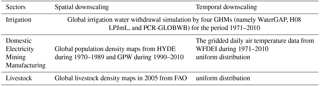
Table 1Datasets for spatial and temporal downscaling of reported water withdrawal by sectors.
The dataset constitutes the first reconstructed global water withdrawal data product at sub-annual (i.e., monthly) and sub-national (i.e., gridded) resolution that is derived from different models and data sources; it was generated by spatially and temporally downscaling country-scale estimates of sectoral water withdrawals from FAO AQUASTAT (and state-scale estimates of USGS for the US). In addition, the industrial sector was disaggregated into manufacturing, mining and cooling of thermal power plants. Downscaling was performed using the output of various models and new modeling approaches. This study adopts the spatial and temporal downscaling methodologies for water withdrawal in previous studies (Wada et al., 2011; Voisin et al., 2013; Hejazi et al., 2014; Wada and Bierkens, 2014), and further validates the temporal downscaling for water withdrawal domestic and electricity generation globally. Thus, with the application of the spatial and temporal downscaling methodologies, a reconstruction of a global monthly gridded water withdrawal dataset for the period 1971–2010 is generated based on multiple reported data sources. Then the spatial and temporal patterns of global water withdrawal by sectors as provided by the newly developed dataset are analyzed. In this paper, data and methods are described in Sect. 2. Section 3 presents the spatiotemporal patterns of water withdrawal by sectors based on the newly developed dataset, and Sect. 4 discusses the uncertainty and limitation of our work. Conclusions are presented in Sect. 5.
2.1 Data
Water withdrawal in the US is obtained from the USGS (http://water.usgs.gov/watuse/) at the state level for every 5 years since 1950, and by sector (irrigation, livestock, domestic, thermoelectric power, mining, and manufacturing). In addition, FAO AQUASTAT provides water withdrawal data for agriculture, irrigation, domestic, and industrial per 5-year interval for 200 countries (http://www.fao.org/nr/water/aquastat/data/query/), and the missing values were filled by Liu et al. (2016) using several techniques such as inverse weighting, linear interpolation, and proxies (e.g., irrigated land area, industrial value added, and population). Water withdrawal for electricity generation, mining, and manufacturing are retrieved from the industrial sector in FAO AQUASTAT in combination with the sectoral water withdrawal simulation of the Global Change Assessment Model (GCAM; Edmonds et al., 1997; Kim et al., 2006). Here, water withdrawal datasets from USGS and FAO AQUASTA, which are used to reconstruct the global gridded monthly water withdrawal dataset, are applied in the US and in the rest of the world, respectively. In this study, irrigation water withdrawal is defined as the water withdrawn for irrigation purposes, and is part of agricultural water withdrawal, together with water withdrawal for livestock (watering and cleaning) and for aquaculture (here lumped as is generally done in existing datasets). According to USGS and FAO definitions (Maupin et al., 2014; FAO, 2016), domestic water withdrawal here represents the water use for indoor household purposes (e.g., drinking, food preparation, bathing, washing clothes and dishes, and flushing toilets), outdoor purposes (e.g., watering lawns and gardens), and for industries and urban agriculture that are connected to the municipal system (e.g., water use by shops, schools, and public buildings). Electricity water withdrawal is the water use for the cooling of thermoelectric and nuclear power plants. Water withdrawal for mining is for the extraction of minerals that may be in the form of solids, liquids, and gases, such as coal, iron, and natural gas. Water withdrawal for manufacturing is for such purposes as fabricating, processing, washing, cooling or transporting a product, incorporating water into a product; or for sanitation needs within the manufacturing facility. These sectoral water withdrawal categories are consistent with the work of Liu et al. (2016).
The datasets used for spatial and temporal downscaling of sectoral water withdrawal are listed in Table 1. Global population density maps, which are applied for spatial downscaling of domestic, electricity generation, mining, and manufacturing sectors, were obtained from the History Database of the Global Environment (HYDE) during 1970–1980 and Gridded Population of the World (GPW) during 1990–2010 in Socioeconomic Data and Application Center (SEDAC). Global livestock density maps for six species (i.e., cattle, buffalo, goat, sheep, pig, and poultry) for the year 2005 were collected from the FAO's Animal Production and Health Division. The gridded daily air temperature data from WATCH Forcing Data methodology applied to ERA-Interim reanalysis data (WFDEI) from 1971 to 2010 is used for temporal downscaling of electricity and domestic water withdrawal from annual to monthly timescales (Weedon et al., 2014). Other sources of air temperature data, from WATCH (Weedon et al., 2010), Princeton (Sheffield et al., 2006), and GSWP3 (Compo et al., 2011), are also adopted to examine the uncertainty in different climate forcing on simulated global monthly water withdrawal for electricity and domestic sectors. In addition, four global gridded monthly irrigation water withdrawal simulations for the period 1971–2010, which are obtained from the Inter-Sectoral Impact Model Inter-comparison Project (ISI-MIP; Warszawski et al., 2014), are utilized for the reconstruction of irrigation water withdrawal. The four products were generated by four GHMs, i.e., WaterGAP (Döll and Siebert, 2002; Alcamo et al., 2003; Döll et al., 2009; Müller Schmied et al., 2014), LPJmL (Rost et al., 2008), H08 (Hanasaki et al., 2008a, b), and PCR-GLOBWB (Van Beek et al., 2011; Wada et al., 2011, 2014), and they are all forced by WFDEI climate data. To investigate the uncertainty derived from forcing data, we also use three other simulated irrigation water withdrawal by WaterGAP forced by three datasets (i.e., Princeton, GSWP3, and WATCH).
2.2 Methodology
Water withdrawal datasets from FAO AQUASTAT and USGS need to be spatially downscaled from country (or state) level to grid scale, and temporally downscaled from a 5-year interval to a monthly scale. As for the irrigation sector, correction factors are used to scale the irrigation water withdrawal estimates by GHMs according to reported data. For the other sectors, the spatial and temporal downscaling is applied to FAO AQUASTA and USGS estimates independently to get the monthly gridded dataset following three steps: firstly the individual sectoral water withdrawal is downscaled from country (or state) level to grid level (0.5∘ × 0.5∘) by using spatial downscaling algorithms, then annual time series of sector water withdrawal is obtained by using linear interpolation between the 5-year interval from reports, and finally a temporal downscaling procedure is adopted to generate monthly gridded water withdrawal data by sector. The sector-specific methodologies for the reconstruction of water withdrawal are described below in detail.
2.2.1 Irrigation
Global gridded monthly irrigation water withdrawals during the period 1971-2010 are generated based on FAO AQUASTAT and USGS estimates and values of gridded monthly irrigation water withdrawals as simulated by four GHMs. Irrigation water withdrawals simulated by these four GHMs all have reasonable agreement (correlation coefficient, r, more than 0.7) with FAO AQUASTAT and USGS estimates at the country level and US state level, respectively (Fig. S1 in the Supplement). Large discrepancies exist among GHMs at the seasonal and regional scales (Fig. S2) due to differences in model structure and parameters (Wada et al., 2013; Liu et al., 2017), so multiple GHMs are taken into account. By applying the correction factors between model estimates and reported estimates to the monthly gridded irrigation water withdrawals simulated by GHMs within a specific country (or state) (i.e., FAO AQUASTAT and USGS datasets), the reconstructed monthly gridded irrigation water withdrawals are calculated as follows:
where Wir is the reconstructed irrigation water withdrawal for the month i of year j at grid g (m3), and Wir_sim is the irrigation water withdrawal for the month i of year j at grid g simulated by four GHMs (m3); fm,p is the correction factor for the simulation by GHMs, calculated by fm,p = Wir_obvWir_simm,p, where Wir_obvm,p and Wir_simm,p are the 5-year irrigation water withdrawal (m3) reported by AQUASTAT (or USGS) and simulated by GHMs, respectively, for country (or state) m (where grid g is located in country m) and time period p (year j is in the period p). Thus, four reconstructed irrigation water withdrawal datasets are generated based on simulations from the four GHMs. The spatial and temporal pattern of the ensemble mean of these four datasets and the disagreement among them are discussed in the results and discussion sections, respectively.
2.2.2 Domestic
The spatial downscaling of domestic water withdrawal follows the methods in Hejazi et al. (2014), which used the population density maps as the proxy for disaggregating domestic water withdrawal from country (or state) level to grid level. A temporal downscaling algorithm for domestic water withdrawal is also used by Wada et al. (2011) and Voisin et al. (2013)
where is domestic water withdrawal in month i of year j (m3); is domestic water withdrawal in year j (m3); Tij is the average temperature in month i of year j; Tavg, Tmax, and Tmin are the average, the maximum, and the minimum monthly temperature in year j (all in ∘C), respectively; parameter R is the amplitude (dimensionless), which measures the relative difference of domestic water withdrawal between the warmest and coldest months in a given year.
Table 2Details of the observed monthly domestic water withdrawal for calibration of parameter R.
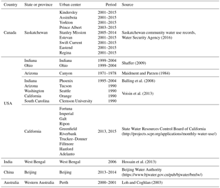
Table 3Calibrated R in different locations and their median value for temporal downscaling of domestic water withdrawal.
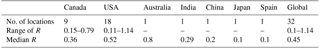
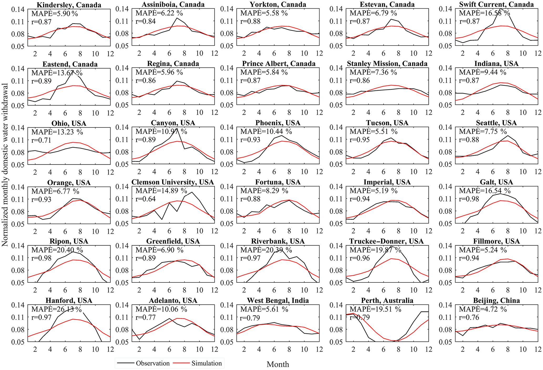
Figure 1Comparison between simulated and observed monthly domestic water withdrawal in 30 global regions: the normalized monthly water withdrawal is the proportion of monthly water withdrawal to the total annual water withdrawal.
Wada et al. (2011) reported that R = 0.1 could fit the variation in domestic water use in Japan and Spain. However, this term is different across regions as domestic water withdrawal is influenced not only by socioeconomic and climatic conditions but also by water policies and strategies (Babel et al., 2007). Here, we use the observed monthly water use data in 30 urban centers and counties (Table 2) to calibrate R in different regions. Table 3 shows the range of calibrated R values for each country, and we use the median value for the temporal downscaling of domestic water withdrawal for the remaining countries with unavailable historical observation. For Japan and Spain we used R = 0.1 as reported by Wada et al. (2011; Table 3). Monthly domestic water withdrawal was calculated using Eq. (2) for the 30 urban centers and counties, and the simulated mean monthly domestic water withdrawal shows reasonable agreement with observations with correlation coefficients (r) of more than 0.8 and mean absolute percentage errors (MAPE) less than 15 % in most urban centers and counties (Fig. 1).
2.2.3 Electricity
Similar to the domestic sector, spatial downscaling of water withdrawal for electricity generation (water withdrawal for cooling of thermal power plants) is based on population density maps (Hejazi et al., 2014). The temporal downscaling of water withdrawal for electricity generation follows Voisin et al. (2013) and Hejazi et al. (2015), which assume that the amount of water withdrawal for electricity generation is proportional to the amount of electricity generated. Here, the generated electricity is assumed to be consumed by three sectors, i.e., building, industry, and transportation. Electricity consumption by building is further divided into three categories: heating, cooling, and other home utilities. Electricity consumption for industry and transportation is assumed to be uniformly distributed within a year, while water withdrawal for building electricity use is dependent on heating degree days (HDD) and cooling degree days (CDD). HDD and CDD, which are derived from outdoor air temperature, are robust indicators for representing heating- and cooling-related energy consumption (Allen, 1976; Karimpour et al., 2014). Here, only electricity use for heating and cooling are assumed to be sensitive to the climatic factors. Equation (3) represents the temporal downscaling of electricity generation from annual to monthly timescales:
where Eij is the electricity use for the month of i and year of j; Ej is the annual electricity use; pb and pit are the proportions of total electricity use for building and transportation and industry together, respectively, with pb + pit = 1; ph, pc and pu are the proportions of total building electricity use for heating, cooling and other home utilities, respectively, with ph + pc + pu = 1; HDDij and CDDij are the HDD and CDD of month i in year j, respectively, and were calculated by using a base temperature of 18 ∘C:
where is the average temperature of the day d of month i in year j. Thus, the monthly water withdrawal for electricity generation is then calculated as follows:
where Wij is the water withdrawal of electricity generation for the month of i and year of j; and Wj is the total annual water withdrawal for electricity generation. The parameters pb, pit, ph, pu and pc are obtained from the International Energy Agency (IEA, 2012a, b). For some counties with low annual CDD (or HDD), there are almost no cooling (or heating) services. However, the parameters pc and ph (the proportions of total building electricity use for cooling and heating, respectively) are not equal to 0, which can lead to a failure in reproducing summer or winter peaks. Thresholds for annual HDD and CDD are defined by assuming that if ∑HDDij < 650 ∘C or ∑CDDij < 450 ∘C, then there is no electricity use for heating or cooling, respectively. Note, thresholds for annual HDD and CDD are obtained by calibration against reported monthly electricity generation data. The monthly water withdrawal for electricity generation is calculated as follows:
If ∑HDDij < 650 and ∑CDDij < 450, then
If ∑HDDij > 650 and ∑CDDij < 450, then
If ∑HDDij < 650 and ∑CDDij > 450, then
If ∑HDDij > 650 and ∑CDDij > 450, then
Voisin et al. (2013) and Hejazi et al. (2015) validated this method against observed data for the year 2005 in the US. To further validate this method globally, monthly electricity generation data during 2000–2012 in 33 OECD countries reported by IEA (http://www.iea.org/statistics/topics/Electricity/) were collected. Figure 2 shows the comparison between simulated and observed monthly mean electricity generation during 2000–2012 in 33 OECD countries. It is found that the simulations agree well (with the correlation coefficient above 0.6 and MAPE under 15 %) with observations in most of the countries. However, electricity generation shows considerable underestimation in summer for some regions (e.g., Austria, Chile, and Switzerland) where hydropower accounts for a large portion of the total electricity generations in summer and parts of electricity are exported to other countries (Bauer, 2009; Wagner et al., 2015; IEA, 2016). In general, the reasonable agreement between simulation and observation suggests the effectiveness of Eqs. (7)–(10) to temporally downscale water withdrawal for electricity generation.
2.2.4 Livestock, mining, and manufacturing
For the spatial downscaling, we apply the global maps of estimated livestock density to downscale water withdrawal of livestock (Alcamo et al., 2003; Hejazi et al., 2014), and population density to downscale water withdrawal of mining and manufacturing sectors. For the temporal downscaling of water withdrawal of livestock, mining, and manufacturing, a uniform distribution (i.e., the monthly value are the same within the year) is adopted following Voisin et al. (2013).
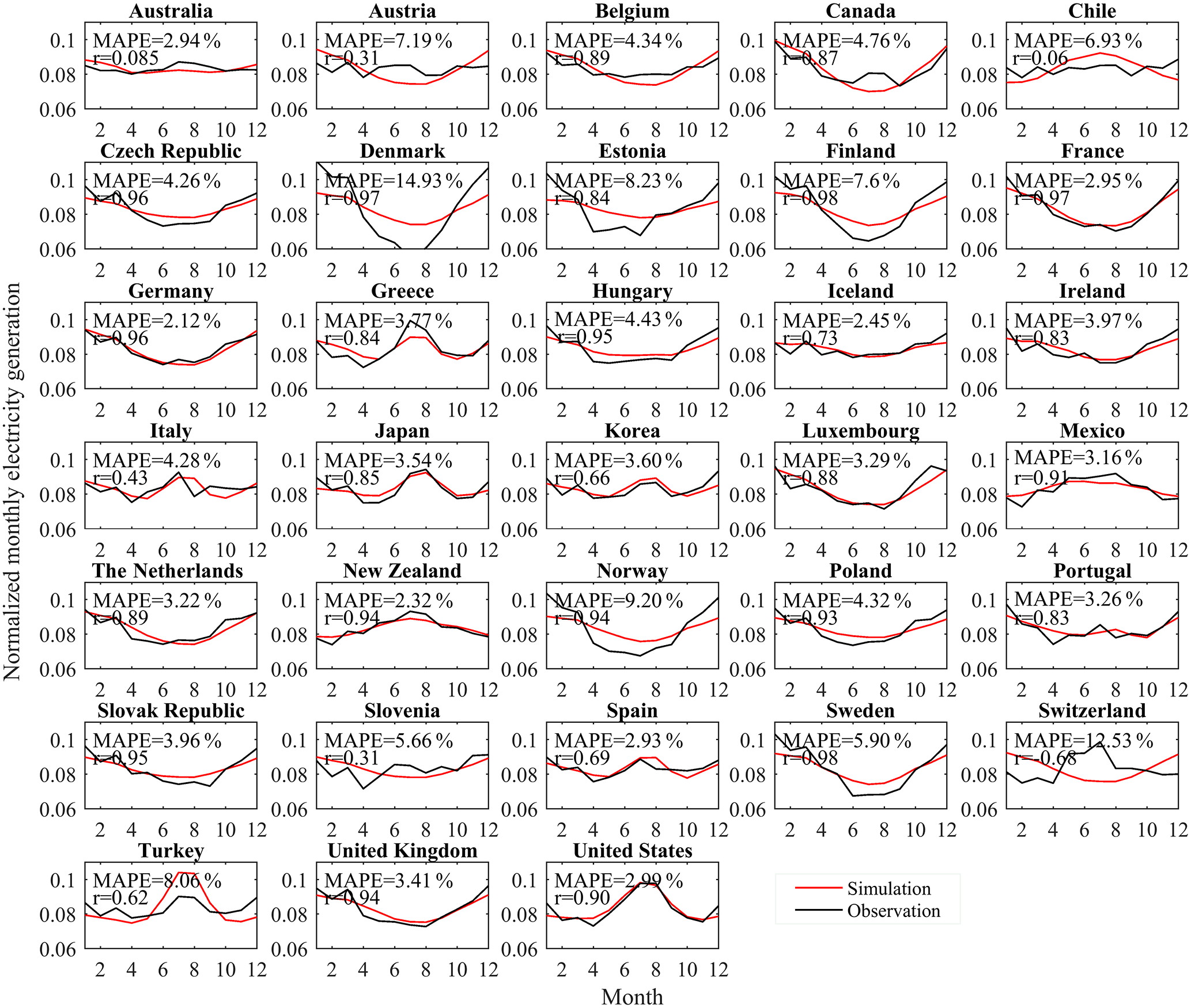
Figure 2Comparison between simulation and observation of normalized monthly mean electricity generation in 33 OECD countries during 2000–2012: the normalized monthly electricity generation is the proportion of monthly electricity generation to the total annual electricity generation.
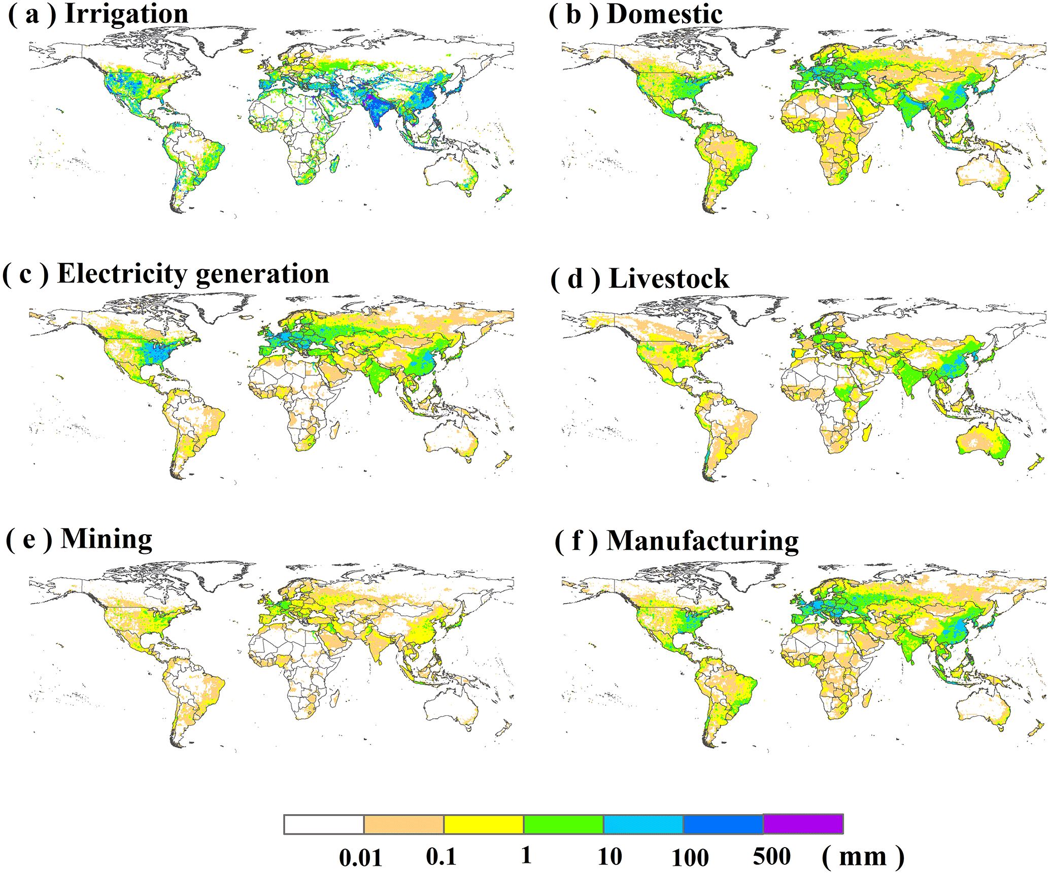
Figure 3Spatial distribution of annual mean water withdrawal by six sectors: (a) irrigation, (b) domestic, (c) electricity generation, (d) livestock, (e) mining, and (f) manufacturing during 1971–2010.
3.1 Spatial distribution of global water withdrawal by sectors
Figure 3 shows the spatial distribution of long-term mean annual water withdrawal by sector during 1971–2010. Total global water withdrawal has increased during the past 40 years, and on average 68 % of global water withdrawal has been used for irrigation, followed by electricity generation (11 %), domestic (9 %), and manufacturing (7 %), while less than 5 % of total global water withdrawal is for livestock and mining purposes (Figs. S3 and S4). Irrigation water withdrawal is highest in the western US, eastern China, and India due to low water availability during the crop growing season and the massive crop productions in these regions. For example, in the western US, the average annual precipitation is less than 400 mm, resulting in water stress for optimal crop growth without irrigation. Different irrigation techniques for crops contribute to the large spatial heterogeneity of water withdrawal (Jägermeyr et al., 2015). For example, large amounts of water are withdrawn for maintaining a certain water level on rice fields in south China and Southeast Asia (Shahid, 2011). In addition, there is almost no irrigation in cold or sparsely populated regions (e.g., north Canada and the Sahara). Domestic water withdrawals are high in the eastern US, eastern China, European countries, coastal regions of South America, and India, but are limited in northern Canada, northern Russia, and the Sahara due to spare population. The spatial distributions of water withdrawal for electricity generation, mining, and manufacturing are broadly similar to that of domestic, and consistent with the global population distribution that water withdrawal regions concentrating in urban areas or regions with denser populations. As for the livestock sector, water withdrawal is mainly used in India, eastern China, and the eastern US where livestock is densely concentrated (Robinson et al., 2014). Generally, the dominant water withdrawal sectors by land area are irrigation in the western US, eastern China, southern Brazil, and India, domestic in northern Brazil and most of Africa, electricity generation in Russia, Canada, and the eastern US, and livestock in Australia (Fig. S3).

Figure 4Relative seasonal distribution of global irrigation water withdrawal over the period 1971–2010 based on the ensemble mean of four GHMs: December to February (DJF), March to May (MAM), June to August (JJA), and September to November (SON), and grids with annual irrigation water withdrawal (AIWW) less than 0.01 mm are not taken into consideration.
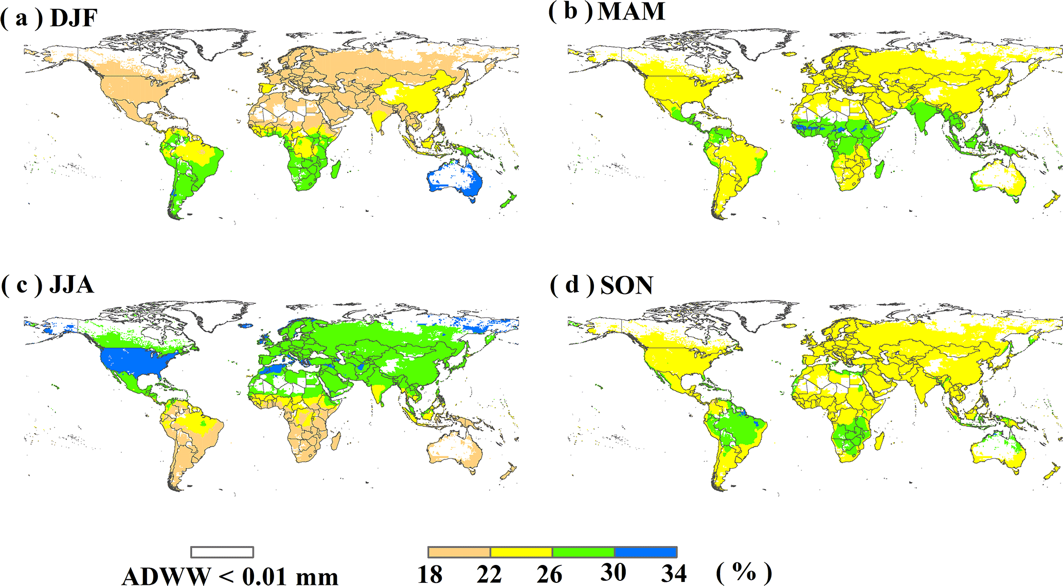
Figure 5Relative seasonal distribution of global domestic water withdrawal over the period 1971–2010: December to February (DJF), March to May (MAM), June to August (JJA), and September to November (SON), and grids with annual domestic water withdrawal (ADWW) less than 0.01 mm are not taken into consideration.
3.2 Seasonal patterns of water withdrawal for irrigation, domestic and electricity generation
An evident seasonal pattern is identified for irrigation water withdrawal during 1971–2010 (Fig. 4), concentrated in June to August (JJA) in the Northern Hemisphere and December to February (DJF) in Southern Hemisphere. In the US and European countries, due to large water requirement in crop growing stages, more than 75 % of annual irrigation water withdrawal occurs in JJA, while no irrigation takes place in DJF. In contrast, in the southern parts of South America and southern Africa, irrigation water is mainly withdrawn in DJF and accounts for about 70 % of total annual irrigation. In general, irrigation water withdrawal exhibits an evident seasonal pattern in mid- and high-latitude regions, but not in the tropical zone (e.g., Brazil and Southeast Asia) where irrigation is applied year-round due mainly to multi-cropping practices. The seasonal variation in irrigation water withdrawal is determined not only by crop calendar but also the climate conditions. For example, in India, most precipitation occurs in rainy seasons (monsoon) but crop water requirement is still large in September to November (SON), leading to a peak of irrigation water withdrawal in SON, especially in northwest India (Rodell et al., 2009; Famiglietti, 2014). The seasonal pattern of domestic water withdrawal (Fig. 5) is largely related to the seasonal temperature variation and the parameter R (i.e., representing the relative difference of domestic water withdrawal between the warmest and coldest months). On both hemispheres, domestic water withdrawal is larger in the respective summer seasons compared to winter, consistent with the seasonal evolution of temperatures. Water withdrawal for lawn and garden, which will take a large part of total domestic water withdrawal in summer, is the dominant factor for the summer peak, especially in developed countries (e.g., the US and Australia; Loh and Coghlan, 2003; Shaffer, 2009). Figure 6 shows the seasonal pattern of water withdrawal for electricity generation. Higher water withdrawal is found in winter than in summer in high-latitude regions (e.g., Canada, western Europe, and southern Australia), where heating is normally adopted in winter while cooling is rarely applied in summer time. On the contrary, electricity for heating is rarely used in winter in tropical regions (e.g., northern Africa and western Asia) as cooling is frequently applied in summer, resulting in dominant water withdrawal for electricity generation in summer. In fact, homes that have air conditioning use electricity as the main source of cooling in the summer, while electricity is also one of the main sources for heating in winter (e.g., the application of furnaces, boiler circulation pumps, and compressors; EIA, 2017), which leads to the summer and winter peak of electricity generation.
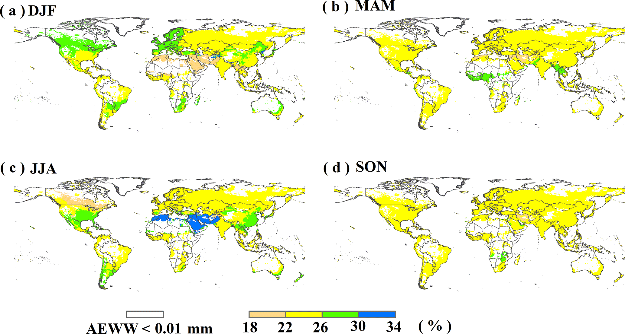
Figure 6Relative seasonal distribution of global electricity generation water withdrawal over the period 1971–2010: December to February (DJF), March to May (MAM), June to August (JJA), and September to November (SON), and grids with annual electricity water withdrawal (AEWW) are not taken into consideration.
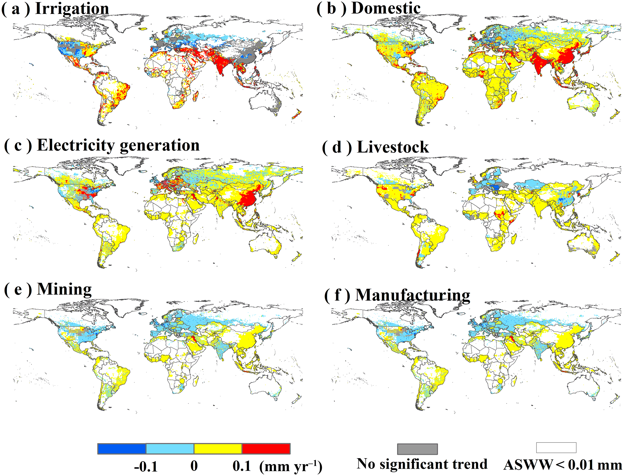
Figure 7Trend of global gridded water withdrawal by sectors: (a) irrigation, (b) domestic, (c) electricity generation, (d) livestock, (e) mining, and (f) manufacturing, grids with annual sectoral water withdrawal (ASWW) less than 0.01 mm are not taken into consideration.
3.3 Trend in water withdrawal during the period 1971–2010 by sectors
Total global water withdrawal has increased significantly from 2500 to 4000 km3 yr−1 during 1971–2010 (Fig. S5). A particularly strong increasing trend is found in China (from ∼ 400 to ∼ 550 km3 yr−1) and India (from ∼ 300 to ∼ 800 km3 yr−1). In contrast, total water withdrawal in the US increased before 1980 but then decreased during 1985–2010, and similar evolution is found for the European Union (EU27). Water withdrawal increased during the past 40 year in most regions (Figs. 7 and S5–S9) as a result of the increasing population, urbanization, the growing food demand, and expansion of irrigated cropland, which are in line with previous studies (Shiklomanov, 2000; Wada and Bierkens, 2014). However, sectoral water withdrawal also shows a decreasing trend in specific regions. Irrigation water withdrawal has exhibited a decreasing trend (about −0.3 mm yr−1) in western US and west Europe, partly due to the application of sprinkler and micro-irrigation systems (Pereira et al., 2002). A significant decreasing trend of domestic water withdrawal is found in most European countries (e.g., Sweden, Germany, and Poland), because of the low growth rate of population and the improvement of domestic water use efficiency and water management (e.g., water price and water meters; Herrington, 1997; Gleick, 2000; Dalhuisen et al., 2003). In addition, some European countries and the US, water withdrawal for electricity generation showed a decreasing trend, which could be attributed to shifts in cooling technologies and fuel mix. For instance, the penetration of more recirculating cooling technologies than once-through, and the shift to less water-intensive fuel mixes (e.g., wind, solar, and natural gas) improved the overall water use efficiency of the electricity sector (Liu et al., 2015).
The reconstructed global gridded monthly water withdrawal dataset by sector is generated by spatially and temporally downscaling country-scale estimates of sectoral water withdrawals from FAOSTAT (and state-scale estimates of USGS for the US). In this section, the uncertainties in the data sources (FAO AQUASTAT and USGS), including model estimates, and in the applied spatial and temporal downscaling methods by sectors are discussed.
4.1 Uncertainties in data sources
Water withdrawal estimates by sectors in the US are provided by the USGS at a high spatial resolution (state and county), and are often treated as a benchmark for model calibration and validation (Vassolo and Döll, 2005; Hejazi et al., 2014; Leng et al., 2016). Water withdrawal estimates from FAO AQUASTAT are mainly from national surveys and assessments (e.g., national yearbook, statistics, and reports) or model simulations (e.g., irrigation water withdrawal). Missing values in the FAO AQUASTAT water withdrawal dataset were filled by Liu et al. (2016) with empirical techniques (e.g., population and irrigated area). Water withdrawals for electricity generation, mining, and manufacturing were broken down from industrial estimates from FAO AQUASTAT with the aid of model simulations. Thus, uncertainties may arise from these procedures. To assess the level of uncertainty in the country-level data, we compared the domestic and industrial water withdrawal time series from 1971 to 2010 with estimates of Flörke et al. (2013) and Shiklomanov (2000; Fig. S10). Global domestic water withdrawal agrees well among these estimates both in trend and average value. Global industrial water withdrawal estimates by Flörke et al. (2013) and Shiklomanov (2000) are higher than estimates used in this study, but they all show a similar changing trend during 1970–2010. Estimates of thermoelectric water withdrawal in this study is lower than estimates from Flörke et al. (2013), and water withdrawal for manufacturing agrees well among these two datasets. In this study, only country-scale estimates from FAO AQUASTAT data and state-scale estimates of USGS for the US are used as basis for downscaling. Future research could explore the collection and consolidation of sub-national and sub-regional sectoral data for other countries or regions, as well as include other sectors beyond the six considered here. For example, water withdrawal for aquaculture is included in livestock, but separating the two sectors can be useful in countries with large freshwater fish production, e.g., China. Other sectors that can be distinguished, include water withdrawal for forestry (e.g., production of papers, furniture) and tourism (e.g., snowmaking, hotels, swimming pools, spas, and golf courses; Cazcarro et al., 2014; Vanham et al., 2009; Vanham, 2016).
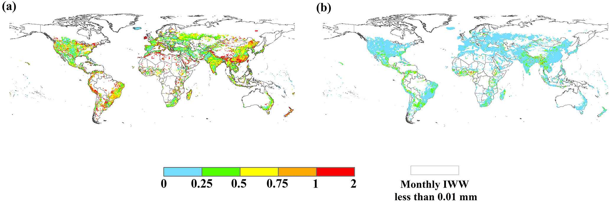
Figure 8Coefficient of variation (CV) in multi-annual average irrigation water withdrawal caused by (a) multi-model framework and by (b) multi-forcing data, and areas with monthly mean irrigation water withdrawal (IWW) less than 0.01 mm are not taken into consideration.
4.2 Uncertainties in reconstructed irrigation water withdrawal
The global gridded monthly irrigation water withdrawal data as produced in this study is based on various data sources, including both census national or state data and model estimates. Specifically, correction factors are used to adjust the irrigation water withdrawal estimates by GHMs to match the reported data at the country or state level. Therefore, besides the reliability of the data source, uncertainties among GHMs and different climate forcing would propagate into the newly developed dataset at the monthly timescale (Wada et al., 2013; Liu et al., 2017). Here, firstly four reconstructed irrigation water withdrawal datasets based on simulations of four GHMs, i.e., WaterGAP, H08, LPJmL, PCR-GLOBWB, forced by WFDEI, are compared to examine the uncertainties induced by model structure; then another four reconstructed irrigation water withdrawal datasets based on simulations of WaterGAP forced by four climatic datasets, namely WFDEI, WATCH, GSWP3, and Princeton, are used to investigate the uncertainties in reconstructed products induced by climate forcing. The coefficient of variation (CV) defined as the standard deviation divided by the ensemble mean value of these four generated datasets are used to evaluate the uncertainty. As shown in Fig. 8, the uncertainties arising from GHMs are rather high (CV > 0.5) in southeast China, the west coast of South America, the southeast of Brazil, and part of the US. Seasonally, CVs in the Northern Hemisphere are larger than those in the Southern Hemisphere in DJF and vice versa in JJA (Fig. S11). Uncertainties among GHMs in irrigation water withdrawal simulation mainly come from the parameterization and assumptions of the irrigation scheme, such as the crop calendar, irrigation area, and crop types (Wada et al., 2016). Although all four GHMs rely on approximately the same dataset of irrigated areas from Siebert et al. (2005; GMIA, http://www.fao.org/nr/water/aquastat/irrigationmap/index.stm), the crop types and the crop calendar definition in these GHMs are different. For example, LPJmL, H08, and WaterGAP use climate conditions to simulate crop calendars (Bondeau et al., 2007; Hanasaki et al., 2010), while PCR-GLOBWB use the crop calendar data from Portmann et al. (2010). In addition, the uncertainty arising from climate forcing is small in most regions (CV < 0.25) due to the high agreement of historical climate datasets (Müller Schmied et al., 2016). Therefore, it is evident that the uncertainty from model structure is larger than that induced by forcing data. To improve the reconstruction of irrigation water withdrawal data, more realistic irrigation parameterization in GHMs and more reliable input data are needed.
4.3 Uncertainties in the spatial and temporal downscaling methods
Although the applied spatial and temporal downscaling methods possess some level of uncertainty in how water withdrawals are distributed spatially within a region or within a year, we did not explore the role of different downscaling methods on the gridded water withdrawal results. Instead we relied on a set of methods that have been used in the literature (Wada et al., 2011; Voisin et al., 2013; Hejazi et al., 2014; Wada and Bierkens, 2014) due to the general lack of multiple methods. Thus, we limit our discussion here to some of the potential sources of uncertainties associated with the spatial and temporal downscaling methods.
The spatial downscaling of water withdrawal by sectors can benefit from considering additional factors to represent the spatial distribution of global water withdrawal. The spatial distribution of domestic water withdrawal is related not only to population density but also to incomes (GDP per capita; Flörke et al., 2013), which varies region by region. Water withdrawal for electricity generation is mainly for cooling purpose in thermoelectric power plants, and can also be affected by many factors besides population, including the location of power plants, the amount of generated electricity, generation type, cooling technology, and fuel type (Byers et al., 2014; Hejazi et al., 2014; Liu et al., 2015). For example, thermoelectric power plants are concentrated outside urban centers, for security reasons (e.g., nuclear power plants) and in proximity to large water quantities (e.g., along rivers). As for mining and manufacturing sectors, Vassolo and Döll (2005) found that the consideration of city nighttime lights works better than urban population. In addition, water withdrawals for manufacturing are also dependent on the location of industry, the purpose for water use (e.g., cleaning, diluting, and cooling), the output type (e.g., food and beverages), the raw materials, and the technical system of water use (Flörke et al., 2013). Thus, future research should also consider using other ancillary data in addition to population density maps for the spatial downscaling of domestic and industrial water withdrawals, such as the geographic locations and characteristics of power plants, manufacturing centers, and mines, and their historical evolutions.
The temporal downscaling methods by sectors can benefit from accounting for the intra-seasonal and inter-annual pattern of water withdrawal inter-annual variation of water withdrawal by sectors needs to be considered when downscaling FAO AQUASTAT and USGS data from of 5-year interval to an annual timescale. The inter-annual variability in human water withdrawal is of great significance for understanding the impacts of climate change (e.g., El Niño–Southern Oscillation, drought, and flood) on human behavior and economy (Vörösmarty et al., 2000; Jacob, 2001; Piao et al., 2010; Haddeland et al., 2014). Furthermore, temporal downscaling of domestic water withdrawal can benefit from considering additional factors besides air temperature , such as precipitation, population, and water availability to represent the seasonality of domestic water withdrawal (White et al., 1972; Hoekstra and Chapagain, 2006). Urban water use characteristics can actually be quite different from rural water characteristics. By only downscaling based upon urban water use characteristics, the reconstructed dataset could thus be biased in rural areas in terms of the temporal pattern. Also, the calibration of the parameter R in this study is rough due to the limitation of reported monthly water withdrawal data. For example, in the two major countries with water withdrawal, China and India, only data from West Bengal and Beijing were available. Given that domestic water withdrawal is roughly 7 % of total water withdrawal in India and 12 % in China, we acknowledge that more data would help improve the temporal downscaling of domestic water withdrawals, and future work should focus on collecting high-resolution water withdrawal data both spatially and temporally. As for electricity generation, the effects of electricity trade and hydropower generation need to be taken into account in future research. Although air temperature datasets used for temporal downscaling may add another source of uncertainty to the reconstructed water withdrawal data, our results show that the uncertainty induced by air temperature datasets is small in the temporal downscaling of water withdrawal for domestic and electricity generation (Fig. S12). This is mainly because of the high agreement in monthly variation in air temperature among the four different data sources (i.e., WFDEI, WATCH, GSWP3, Princeton) as all of them are bias corrected to (different) versions of the Climatic Research Unit (CRU) time series (Müller Schmied et al., 2016). For livestock, mining, and manufacturing sectors, uniform distribution is applied for temporal downscaling. Incorporating the sub-annual variations in these sectors would require collecting monthly water withdrawal datasets to establish formulas that relate monthly water withdrawal for livestock, mining, and manufacturing to climate signals (e.g., temperature, precipitation).
In this study, a reconstructed global gridded monthly sectoral water withdrawal dataset, which is open access online (https://doi.org/10.5281/zenodo.1209296), was produced for the period 1971–2010 by temporally and spatially downscaling country-level (FAO AQUASTAT) and state-level (USGS, only for USA) datasets using various models and new modeling approaches. Correction factors are used to scale irrigation water withdrawal estimates by GHMs to annual country (or state) estimates from FAO and USGS. Global population density maps are used for the spatial downscaling for water withdrawal for domestic, electricity generation, mining, and manufacturing; while livestock density maps are used for the livestock sector. In addition, air temperature is used to present the monthly variation in water withdrawal by domestic and electricity generation, which are validated against observations, and simulation results show reasonable agreements with observations in selected regions.
The reconstructed dataset, at 0.5∘ spatial resolution and monthly temporal resolution, includes water withdrawal by sector, i.e., irrigation, domestic, electricity generation, livestock, mining, and manufacturing. Based on the reconstructed dataset, the spatial and temporal change patterns of global water withdrawal by sectors were analyzed. Globally, most water withdrawal is used for irrigation, followed by electricity generation and domestic. Spatially, the dominant irrigation water withdrawal areas are regions with large irrigated cropland and massive crop productions, e.g., the western US, eastern China, and India. Water withdrawal for domestic, electricity generation, mining, and manufacturing are high in urban areas or regions with denser populations. Seasonally, irrigation water withdrawal exhibits an evident seasonal pattern in mid- and high-latitude regions, but not in the tropical zone. Domestic water withdrawal is larger in JJA than in DJF in the Northern Hemisphere, and vice versa in the Southern Hemisphere. Water withdrawal for electricity generation showed a winter peak in high-latitude regions and a summer peak in low-latitude regions.
In addition, the uncertainties in the reconstructed water withdrawal data are analyzed, and limitations for spatial and temporal downscaling of other sectors are discussed. Results show that the uncertainties arising from model structure are larger than that induced by forcing data in the reconstructed irrigation water withdrawal. More advanced models that capture the spatial pattern and intra- and inter-annual variabilities in sectoral water withdrawal are needed, and more frequently and spatially resolved observed water withdrawal data at the country or region scale are also required for improving the quality of the reconstructed dataset. In whole, despite the uncertainties and limitations, this study is of great significance not only for cross-comparison and validation for modeling and analyzing the impacts of human water use but also for investigating water-use-related issues at finer spatial, temporal, and sectoral scales.
Water withdrawal data in the US are obtained from the USGS (http://water.usgs.gov/watuse/), and water withdrawal data for agriculture, irrigation, domestic, and industrial sectors for 200 global countries are from FAO AQUASTAT (http://www.fao.org/nr/water/aquastat/data/query/). Historical global population density map data were obtained from the History Database of the Global Environment (HYDE) during 1970–1980 (http://themasites.pbl.nl/tridion/en/themasites/hyde/) and Gridded Population of the World (GPW) during 1990–2010 in the Socioeconomic Data and Application Center (SEDAC) (http://sedac.ciesin.columbia.edu/). Global livestock density maps for the year 2005 were collected from the FAO's Animal Production and Health Division (http://www.fao.org/ag/againfo/resources/en/glw/GLW_dens). Climate data and model outputs of GHMs were provided by the Inter-Sectoral Impact Model Inter-comparison Project (https://www.isimip.org).
The supplement related to this article is available online at: https://doi.org/10.5194/hess-22-2117-2018-supplement.
The authors declare that they have no conflict of interest.
This research was supported by the Office of Science of the US Department of
Energy through the Multi-Sector Dynamics, Earth and Environmental System Modeling
Program. PNNL is operated for DOE by the Battelle Memorial Institute under
contract DE-AC05-76RL01830. Support from the National Natural Science Foundation
of China (41730645, 41790424, and 41425002) are also acknowledged.
Edited by: Nadia Ursino
Reviewed by: three anonymous referees
Adams, R. M., Rosenzweig, C., Peart, R., Ritchie, J. T., and McCarl, B. A.: Global climate change and US agriculture, Nature, 345, 219–224, 1990.
Alcamo, J., Döll, P., Henrichs, T., Kaspar, F., Lehner, B., Rösch, T., and Siebert, S.: Development and testing of the WaterGAP 2 global model of water use and availability, Hydrolog. Sci. J., 48, 317–337, 2003.
Allen, J. C.: A modified sine wave method for calculating degree days, Environ. Entomol., 5, 388–396, 1976.
Babel, M., Gupta, A. D., and Pradhan, P.: A multivariate econometric approach for domestic water demand modeling: an application to Kathmandu, Nepal, Water Resour. Manage., 21, 573–589, 2007.
Balling, R. C., Gober, P., and Jones, N.: Sensitivity of residential water consumption to variations in climate: an intraurban analysis of Phoenix, Arizona, Water Resour. Res., 44, W10401, https://doi.org/10.1029/2007WR006722, 2008.
Barnett, T. P., Adam, J. C., and Lettenmaier, D. P.: Potential impacts of a warming climate on water availability in snow-dominated regions, Nature, 438, 303–309, 2005.
Bauer, C. J.: Dams and markets: Rivers and electric power in Chile, Nat. Resour. J., 49, 583–691, 2009.
Bondeau, A., Smith, P. C., Zaehle, S., Schaphoff, S., Lucht, W., Cramer, W., Gerten, D., Lotze Campen, H., Müller, C., and Reichstein, M.: Modelling the role of agriculture for the 20th century global terrestrial carbon balance, Global Change Biol., 13, 679–706, 2007.
Boucher, O., Myhre, G., and Myhre, A.: Direct human influence of irrigation on atmospheric water vapour and climate, Clim. Dynam., 22, 597–603, 2004.
Byers, E. A., Hall, J. W., and Amezaga, J. M.: Electricity generation and cooling water use: UK pathways to 2050, Global Environ. Change, 25, 16–30, 2014.
Cazcarro, I., Hoekstra, A. Y., and Chóliz, J. S.: The water footprint of tourism in Spain, Tourism Manage., 40, 90–101, 2014.
Compo, G. P., Whitaker, J. S., Sardeshmukh, P. D., Matsui, N., Allan, R. J., Yin, X., Gleason, B. E., Vose, R. S., Rutledge, G., and Bessemoulin, P.: The twentieth century reanalysis project, Q. J. Roy. Meteorol. Soc., 137, 1–28, 2011.
Dalhuisen, J. M., Florax, R. J., De Groot, H. L., and Nijkamp, P.: Price and income elasticities of residential water demand: a meta-analysis, Land Econ., 79, 292–308, 2003.
DeAngelis, A., Dominguez, F., Fan, Y., Robock, A., Kustu, M. D., and Robinson, D.: Evidence of enhanced precipitation due to irrigation over the Great Plains of the United States, J. Geophys. Res.-Atmos., 115, D15115, https://doi.org/10.1029/2010JD013892, 2010.
Döll, P. and Siebert, S.: Global modeling of irrigation water requirements, Water Resour. Res., 38, 1037, https://doi.org/10.1029/2001WR000355, 2002.
Döll, P., Fiedler, K., and Zhang, J.: Global-scale analysis of river flow alterations due to water withdrawals and reservoirs, Hydrol. Earth Syst. Sci., 13, 2413–2432, https://doi.org/10.5194/hess-13-2413-2009, 2009.
Döll, P., Hoffmann-Dobrev, H., Portmann, F. T., Siebert, S., Eicker, A., Rodell, M., Strassberg, G., and Scanlon, B.: Impact of water withdrawals from groundwater and surface water on continental water storage variations, J. Geodyn., 59, 143–156, 2012.
Döll, P., Müller Schmied, H., Schuh, C., Portmann, F. T., and Eicker, A.: Global-scale assessment of groundwater depletion and related groundwater abstractions: Combining hydrological modeling with information from well observations and GRACE satellites, Water Resour. Res., 50, 5698–5720, 2014.
Edmonds, J., Wise, M., Pitcher, H., Richels, R., Wigley, T., and Maccracken, C.: An integrated assessment of climate change and the accelerated introduction of advanced energy technologies, Mitig. Adapt. Strat. Global Change, 1, 311–339, 1997.
EIA: Electric Power Monthly with Data for May 2017, US Energy Information Administration (EIA), Washington, D.C., 2017.
Famiglietti, J.: The global groundwater crisis, Nat. Clim. Change, 4, 945–948, 2014.
FAO: AQUASTAT Main Database, Food and Agriculture Organization of the United Nations (FAO), http://www.fao.org/nr/water/aquastat/data/query/index.html?lang=en (last access: 28 March 2018), 2016.
Flörke, M., Kynast, E., Bärlund, I., Eisner, S., Wimmer, F., and Alcamo, J.: Domestic and industrial water uses of the past 60 years as a mirror of socio-economic development: A global simulation study, Global Environ. Change, 23, 144–156, 2013.
Gleick, P. H.: A look at twenty-first century water resources development, Water Int., 25, 127–138, 2000.
Haddeland, I., Lettenmaier, D. P., and Skaugen, T.: Effects of irrigation on the water and energy balances of the Colorado and Mekong river basins, J. Hydrol., 324, 210–223, 2006.
Haddeland, I., Heinke, J., Biemans, H., Eisner, S., Flörke, M., Hanasaki, N., Konzmann, M., Ludwig, F., Masaki, Y., and Schewe, J.: Global water resources affected by human interventions and climate change, P. Natl. Acad. Sci. USA, 111, 3251–3256, 2014.
Hanasaki, N., Kanae, S., Oki, T., Masuda, K., Motoya, K., Shirakawa, N., Shen, Y., and Tanaka, K.: An integrated model for the assessment of global water resources – Part 1: Model description and input meteorological forcing, Hydrol. Earth Syst. Sci., 12, 1007–1025, https://doi.org/10.5194/hess-12-1007-2008, 2008a.
Hanasaki, N., Kanae, S., Oki, T., Masuda, K., Motoya, K., Shirakawa, N., Shen, Y., and Tanaka, K.: An integrated model for the assessment of global water resources – Part 2: Applications and assessments, Hydrol. Earth Syst. Sci., 12, 1027–1037, https://doi.org/10.5194/hess-12-1027-2008, 2008b.
Hanasaki, N., Inuzuka, T., Kanae, S., and Oki, T.: An estimation of global virtual water flow and sources of water withdrawal for major crops and livestock products using a global hydrological model, J. Hydrol., 384, 232–244, 2010.
Hejazi, M., Edmonds, J., Clarke, L., Kyle, P., Davies, E., Chaturvedi, V., Wise, M., Patel, P., Eom, J., and Calvin, K.: Long-term global water projections using six socioeconomic scenarios in an integrated assessment modeling framework, Technol. Forecast. Social Change, 81, 205–226, 2014.
Hejazi, M. I., Voisin, N., Liu, L., Bramer, L. M., Fortin, D. C., Hathaway, J. E., Huang, M., Kyle, P., Leung, L. R., and Li, H.-Y.: 21st century United States emissions mitigation could increase water stress more than the climate change it is mitigating, P. Natl. Acad. Sci. USA, 112, 10635–10640, 2015.
Herrington, P.: Pricing water properly, in: Ecotaxation, edited by: O'Riordan, T., Earthscan, London, 263–286, 1997.
Hoekstra, A. Y. and Chapagain, A. K.: Water footprints of nations: water use by people as a function of their consumption pattern, Water Resour. Manage., 1, 35–48, 2006.
Hossain, M. A., Rahman, M. M., Murrill, M., Das, B., Roy, B., Dey, S., Maity, D., and Chakraborti, D.: Water consumption patterns and factors contributing to water consumption in arsenic affected population of rural West Bengal, India, Sci. Total Environ., 463, 1217–1224, 2013.
IEA: Energy Balances of OECD Countries 1960–2010, 2012 Edn., International Energy Agency, Paris, 2012a.
IEA: Energy Balances of non-OECD Countries 1971–2010, 2012 Edn., International Energy Agency, Paris, 2012b.
IEA: IEA statistics: Monthly electricity statistics, International Energy Agency, Paris, 2016.
Jacob, D.: A note to the simulation of the annual and inter-annual variability of the water budget over the Baltic Sea drainage basin, Meteorol. Atmos. Phys., 77, 61–73, 2001.
Jägermeyr, J., Gerten, D., Heinke, J., Schaphoff, S., Kummu, M., and Lucht, W.: Water savings potentials of irrigation systems: global simulation of processes and linkages, Hydrol. Earth Syst. Sci., 19, 3073–3091, https://doi.org/10.5194/hess-19-3073-2015, 2015.
Karimpour, M., Belusko, M., Xing, K., and Bruno, F.: Minimising the life cycle energy of buildings: Review and analysis, Build. Environ., 73, 106–114, 2014.
Kim, S. H., Edmonds, J., Lurz, J., Smith, S. J., and Wise, M.: The objECTS Framework for integrated Assessment: Hybrid Modeling of Transportation, Energy J., 27, 63–91, 2006.
Kueppers, L. M., Snyder, M. A., and Sloan, L. C.: Irrigation cooling effect: Regional climate forcing by land-use change, Geophys. Res. Lett., 34, L03703, https://doi.org/10.1029/2006GL028679, 2007.
Kustu, M. D., Fan, Y., and Rodell, M.: Possible link between irrigation in the US High Plains and increased summer streamflow in the Midwest, Water Resour. Res., 47, W03522, https://doi.org/10.1029/2010WR010046, 2011.
Leng, G., Zhang, X., Huang, M., Yang, Q., Rafique, R., Asrar, G. R., and Ruby Leung, L.: Simulating county-level crop yields in the Conterminous United States using the Community Land Model: The effects of optimizing irrigation and fertilization, J. Adv. Model. Earth Syst., 8, 1912–1931, 2016.
Liu, L., Hejazi, M., Patel, P., Kyle, P., Davies, E., Zhou, Y., Clarke, L., and Edmonds, J.: Water demands for electricity generation in the US: Modeling different scenarios for the water–energy nexus, Technol. Forecast. Social Change, 94, 318–334, 2015.
Liu, X., Tang, Q., Cui, H., Mu, M., Gerten, D., Gosling, S. N., Masaki, Y., Satoh, Y., and Wada, Y.: Multimodel uncertainty changes in simulated river flows induced by human impact parameterizations, Environ. Res. Lett., 12, 025009, https://doi.org/10.1088/1748-9326/aa5a3a, 2017.
Liu, Y., Hejazi, M., Kyle, P., Kim, S. H., Davies, E., Miralles, D. G., Teuling, A. J., He, Y., and Niyogi, D.: Global and regional evaluation of energy for water, Environ. Sci. Technol., 50, 9736–9745, 2016.
Lobell, D., Bala, G., Mirin, A., Phillips, T., Maxwell, R., and Rotman, D.: Regional differences in the influence of irrigation on climate, J. Climate, 22, 2248–2255, 2009.
Loh, M. and Coghlan, P.: Domestic water use study in Perth, Western Australia 1998–2001, Water Corporation of Western Australia, Perth, 2003.
Maidment, D. R. and Parzen, E.: Cascade model of monthly municipal water use, Water Resour. Res., 20, 15–23, 1984.
Maupin, M. A., Kenny, J. F., Hutson, S. S., Lovelace, J. K., Barber, N. L., and Linsey, K. S.: Estimated use of water in the United States in 2010, US Geological Survey Circular 1405, US Geological Survey, Reston, p. 56, 2014.
Müller Schmied, H., Eisner, S., Franz, D., Wattenbach, M., Portmann, F. T., Flörke, M., and Döll, P.: Sensitivity of simulated global-scale freshwater fluxes and storages to input data, hydrological model structure, human water use and calibration, Hydrol. Earth Syst. Sci., 18, 3511–3538, https://doi.org/10.5194/hess-18-3511-2014, 2014.
Müller Schmied, H., Adam, L., Eisner, S., Fink, G., Flörke, M., Kim, H., Oki, T., Portmann, F. T., Reinecke, R., Riedel, C., Song, Q., Zhang, J., and Döll, P.: Variations of global and continental water balance components as impacted by climate forcing uncertainty and human water use, Hydrol. Earth Syst. Sci., 20, 2877–2898, https://doi.org/10.5194/hess-20-2877-2016, 2016.
Pereira, L. S., Oweis, T., and Zairi, A.: Irrigation management under water scarcity, Agr. Water Manage., 57, 175–206, 2002.
Piao, S., Ciais, P., Huang, Y., Shen, Z., Peng, S., Li, J., Zhou, L., Liu, H., Ma, Y., and Ding, Y.: The impacts of climate change on water resources and agriculture in China, Nature, 467, 43–51, 2010.
Pokhrel, Y., Hanasaki, N., Koirala, S., Cho, J., Yeh, P. J.-F., Kim, H., Kanae, S., and Oki, T.: Incorporating anthropogenic water regulation modules into a land surface model, J. Hydrometeorol., 13, 255–269, 2012.
Portmann, F. T., Siebert, S., and Döll, P.: MIRCA2000 – Global monthly irrigated and rainfed crop areas around the year 2000: A new high-resolution data set for agricultural and hydrological modeling, Global Biogeochem. Cy., 24, GB1011, https://doi.org/10.1029/2008GB003435, 2010.
Robinson, T. P., Wint, G. W., Conchedda, G., Van Boeckel, T. P., Ercoli, V., Palamara, E., Cinardi, G., D'Aietti, L., Hay, S. I., and Gilbert, M.: Mapping the global distribution of livestock, PloS One, 9, e96084, https://doi.org/10.1371/journal.pone.0096084, 2014.
Rodell, M., Velicogna, I., and Famiglietti, J. S.: Satellite-based estimates of groundwater depletion in India, Nature, 460, 999–1002, 2009.
Rost, S., Gerten, D., Bondeau, A., Lucht, W., Rohwer, J., and Schaphoff, S.: Agricultural green and blue water consumption and its influence on the global water system, Water Resour. Res., 44, W09405, https://doi.org/10.1029/2007WR006331, 2008.
Shaffer, K.: Variations in Withdrawal, Return Flow, and Consumptive Use of Water in Ohio and Indiana, with Selected Data from Wisconsin, 1999–2004, US Geological Survey, Reston, 2009.
Shahid, S.: Impact of climate change on irrigation water demand of dry season Boro rice in northwest Bangladesh, Climatic Change, 105, 433–453, 2011.
Sheffield, J., Goteti, G., and Wood, E. F.: Development of a 50-year high-resolution global dataset of meteorological forcings for land surface modeling, J. Climate, 19, 3088–3111, 2006.
Shiklomanov, I. A.: Appraisal and assessment of world water resources, Water Int., 25, 11–32, 2000.
Shiklomanov, I. A. and Rodda, J. C.: World Water Resources at the Beginning of the 21st Century, International Hydrology Series, Cambridge University Press, Cambridge, UK, 2003.
Siebert, S., Döll, P., Hoogeveen, J., Faures, J.-M., Frenken, K., and Feick, S.: Development and validation of the global map of irrigation areas, Hydrol. Earth Syst. Sci., 9, 535–547, https://doi.org/10.5194/hess-9-535-2005, 2005.
Stohlgren, T. J., Chase, T. N., Pielke, R. A., Kittel, T. G., and Baron, J.: Evidence that local land use practices influence regional climate, vegetation, and stream flow patterns in adjacent natural areas, Global Change Biol., 4, 495–504, 1998.
Tang, Q., Oki, T., Kanae, S., and Hu, H.: The influence of precipitation variability and partial irrigation within grid cells on a hydrological simulation, J. Hydrometeorol., 8, 499–512, 2007.
Tang, Q., Oki, T., Kanae, S., and Hu, H.: Hydrological cycles change in the Yellow River basin during the last half of the twentieth century, J. Climate, 21, 1790–1806, 2008.
Taylor, R. G., Scanlon, B., Döll, P., Rodell, M., Van Beek, R., Wada, Y., Longuevergne, L., Leblanc, M., Famiglietti, J. S., and Edmunds, M.: Ground water and climate change, Nat. Clim. Change, 3, 322–329, 2013.
Van Beek, L., Wada, Y., and Bierkens, M. F.: Global monthly water stress: 1. Water balance and water availability, Water Resour. Res., 47, W07517, https://doi.org/10.1029/2010WR009791, 2011.
Vanham, D.: Does the water footprint concept provide relevant information to address the water–food–energy–ecosystem nexus?, Ecosyst. Serv., 17, 298–307, 2016.
Vanham, D., Fleischhacker, E., and Rauch, W.: Impact of snowmaking on alpine water resources management under present and climate change conditions, Water Sci. Technol., 59, 1793–801, 2009.
Vassolo, S. and Döll, P.: Global-scale gridded estimates of thermoelectric power and manufacturing water use, Water Resour. Res., 41, W04010, https://doi.org/10.1029/2004WR003360, 2005.
Voisin, N., Liu, L., Hejazi, M., Tesfa, T., Li, H., Huang, M., Liu, Y., and Leung, L. R.: One-way coupling of an integrated assessment model and a water resources model: evaluation and implications of future changes over the US Midwest, Hydrol. Earth Syst. Sci., 17, 4555–4575, https://doi.org/10.5194/hess-17-4555-2013, 2013.
Vörösmarty, C. J., Green, P., Salisbury, J., and Lammers, R. B.: Global water resources: vulnerability from climate change and population growth, Science, 289, 284–288, 2000.
Wada, Y. and Bierkens, M. F.: Sustainability of global water use: past reconstruction and future projections, Environ. Res. Lett., 9, 104003, W07518, https://doi.org/10.1029/2010WR009792, 2014.
Wada, Y., Van Beek, L., Viviroli, D., Dürr, H. H., Weingartner, R., and Bierkens, M. F.: Global monthly water stress: 2. Water demand and severity of water stress, Water Resour. Res., 47, W00J12, https://doi.org/10.1029/2010WR010283, 2011.
Wada, Y., Wisser, D., Eisner, S., Flörke, M., Gerten, D., Haddeland, I., Hanasaki, N., Masaki, Y., Portmann, F. T., and Stacke, T.: Multimodel projections and uncertainties of irrigation water demand under climate change, Geophys. Res. Lett., 40, 4626–4632, 2013.
Wada, Y., Wisser, D., and Bierkens, M. F. P.: Global modeling of withdrawal, allocation and consumptive use of surface water and groundwater resources, Earth Syst. Dynam., 5, 15–40, https://doi.org/10.5194/esd-5-15-2014, 2014.
Wada, Y., Flörke, M., Hanasaki, N., Eisner, S., Fischer, G., Tramberend, S., Satoh, Y., van Vliet, M. T. H., Yillia, P., Ringler, C., Burek, P., and Wiberg, D.: Modeling global water use for the 21st century: the Water Futures and Solutions (WFaS) initiative and its approaches, Geosci. Model Dev., 9, 175–222, https://doi.org/10.5194/gmd-9-175-2016, 2016.
Wagner, B., Hauer, C., Schoder, A., and Habersack, H.: A review of hydropower in Austria: Past, present and future development, Renew. Sustain. Energy Rev., 50, 304–314, 2015.
Wang, D. and Hejazi, M.: Quantifying the relative contribution of the climate and direct human impacts on mean annual streamflow in the contiguous United States, Water Resour. Res., 47, W00J12, https://doi.org/10.1029/2010WR010283, 2011.
Warszawski, L., Frieler, K., Huber, V., Piontek, F., Serdeczny, O., and Schewe, J.: The inter-sectoral impact model intercomparison project (ISI–MIP): project framework, P. Natl. Acad. Sci. USA, 111, 3228–3232, 2014.
Water Security Agency: Saskatchewan Community Water use Records 2001 to 2015, Report 29, The Water Security Agency, Moose Jaw, Saskatchewan, 2016.
Weedon, G. P., Gomes, S., Viterbo, P., Osterle, H., Adam, J. C., Bellouin, N., Boucher, O., and Best, M.: The WATCH forcing data 1958–2001: a meteorological forcing dataset for land surface- and hydrological-models, WATCH technical report, available at: http://www.eu-watch.org/publications/technical-reports (last access: March 2018), 2010.
Weedon, G. P., Balsamo, G., Bellouin, N., Gomes, S., Best, M. J., and Viterbo, P.: The WFDEI meteorological forcing data set: WATCH Forcing Data methodology applied to ERA-Interim reanalysis data, Water Resour. Res., 50, 7505–7514, 2014.
White, G. F., Bradley, D. J., and White, A. U.: Drawers of water. Domestic water use in East Africa, University of Chicago Press, Chicago, Illinois, 1972.
Yin, Y., Tang, Q., Liu, X., and Zhang, X.: Water scarcity under various socio-economic pathways and its potential effects on food production in the Yellow River basin, Hydrol. Earth Syst. Sci., 21, 791–804, https://doi.org/10.5194/hess-21-791-2017, 2017.