the Creative Commons Attribution 3.0 License.
the Creative Commons Attribution 3.0 License.
Numerical modeling and sensitivity analysis of seawater intrusion in a dual-permeability coastal karst aquifer with conduit networks
Bill X. Hu
Ming Ye
Long-distance seawater intrusion has been widely observed through the subsurface conduit system in coastal karst aquifers as a source of groundwater contaminant. In this study, seawater intrusion in a dual-permeability karst aquifer with conduit networks is studied by the two-dimensional density-dependent flow and transport SEAWAT model. Local and global sensitivity analyses are used to evaluate the impacts of boundary conditions and hydrological characteristics on modeling seawater intrusion in a karst aquifer, including hydraulic conductivity, effective porosity, specific storage, and dispersivity of the conduit network and of the porous medium. The local sensitivity analysis evaluates the parameters' sensitivities for modeling seawater intrusion, specifically in the Woodville Karst Plain (WKP). A more comprehensive interpretation of parameter sensitivities, including the nonlinear relationship between simulations and parameters, and/or parameter interactions, is addressed in the global sensitivity analysis. The conduit parameters and boundary conditions are important to the simulations in the porous medium because of the dynamical exchanges between the two systems. The sensitivity study indicates that salinity and head simulations in the karst features, such as the conduit system and submarine springs, are critical for understanding seawater intrusion in a coastal karst aquifer. The evaluation of hydraulic conductivity sensitivity in the continuum SEAWAT model may be biased since the conduit flow velocity is not accurately calculated by Darcy's equation as a function of head difference and hydraulic conductivity. In addition, dispersivity is no longer an important parameter in an advection-dominated karst aquifer with a conduit system, compared to the sensitivity results in a porous medium aquifer. In the end, the extents of seawater intrusion are quantitatively evaluated and measured under different scenarios with the variabilities of important parameters identified from sensitivity results, including salinity at the submarine spring with rainfall recharge, sea level rise, and a longer simulation time under an extended low rainfall period.


Many serious environmental issues have been caused by seawater intrusion in coastal regions, such as soil salinization, marine and estuarine ecological changes, and groundwater contamination (Bear, 1999). Werner et al. (2013) pointed out that climate variations, groundwater pumping, and fluctuating sea levels are important factors in the mixing of seawater and freshwater in the aquifer. Custodio (1987) and Shoemaker (2004) summarized the control factors of seawater intrusion into a coastal aquifer, including the geologic and lithological heterogeneity, localized surface recharge, paleohydrogeological conditions, and anthropogenic influences. Particularly, seawater intrusion in a coastal aquifer is significantly impacted by sea level rise, which has been recognized as a serious environmental threat in the 21st century (Voss and Souza, 1987; Bear, 1999; IPCC, 2007). In the Ghyben–Herzberg relationship, a small rise of sea level causes extended seawater intrusion and significantly moves the mixing interface position further landward in a coastal aquifer (Werner and Simmons, 2009). For example, Essink et al. (2010) systematically studied the exacerbated seawater intrusion under sea level rise and global climate change. Likewise, high tides associated with hurricanes or tropical storms have been found to temporarily affect the extent of seawater intrusion in a coastal aquifer (Moore and Wilson, 2005; Wilson et al., 2011).
Modeling seawater intrusion in a coastal aquifer requires a coupled density-dependent flow and salt transport groundwater model. The simulated salinity is computed by the groundwater velocity field from flow modeling, and salinity in turn determines water density and affects the simulation of flow field. Several variable-density numerical models have been developed and widely used to study seawater intrusion, including SUTRA (Voss and Provost, 1984) and FEFLOW (Diersch, 2002). SEAWAT is a widely used density-dependent model, which solves flow equations with a finite difference method and transport equations with three major classes of numerical techniques (Guo and Langevin, 2002; Langevin et al., 2003). Generally speaking, most variable-density models are numerically complicated and computationally expensive. These models require a smaller timestep and an implicit procedure for solving flow and transport equations iteratively many times in each timestep (Werner et al., 2013).
In addition, a karst aquifer is particularly vulnerable to groundwater contamination including seawater intrusion in a coastal region since sinkholes and karst windows are usually connected by well-developed subsurface conduit networks. Some karst caves are found open to the sea and become submarine springs below sea level, connected with the conduit network as natural pathways for seawater intrusion. Fleury et al. (2007) reviewed the studies of freshwater discharge and seawater intrusion through karst conduits and submarine springs in coastal karst aquifers, and they summarized the important control factors, including the hydraulic gradient of the equivalent freshwater head, hydraulic conductivity, and seasonal precipitation variation. For example, seawater intrudes through the conduit network as preferential flow and contaminates the fresh groundwater resources in a coastal karst aquifer (Calvache and Pulido-Bosch, 1997). As an indicator of rainfall and regional freshwater recharges, salinity at the outlet of a conduit system is diluted by freshwater discharge during a rainfall season, but it remains constant as saline water during a low rainfall period (Martin and Dean, 2001; Martin et al., 2012).
Modeling groundwater flow in a dual-permeability karst aquifer is a challenging issue since groundwater flow in a karst conduit system is often non-laminar (Davis, 1996; Shoemaker et al., 2008; Gallegos et al., 2013). Several discrete-continuum numerical models, such as MODFLOW-CFPM1 (Shoemaker et al., 2008) and CFPv2 (Reimann et al., 2014, 2013; Xu et al., 2015a, b), have been developed to simultaneously solve the non-laminar flow in the conduit, the Darcian flow in a porous medium, and the exchanges between the two systems. However, these constant-density karst models have limitations in simulating the density-dependent seawater intrusion processes in a coastal aquifer. The VDFST-CFP, developed by Xu and Hu (2017), is based on a density-dependent discrete-continuum modeling approach to study seawater intrusion in a coastal karst aquifer with conduits. However, VDFST-CFP is not able to simulate the seawater intrusion processes addressed in this study due to the computational constraints and the numerical method limitations associated with the aquifer geometry and the domain scale. Therefore, the variable-density SEAWAT model is still applied in this study, in which Darcy's equation is used to compute flow not only in the porous medium, but also in the conduit with large values of hydraulic conductivity and effective porosity.
Since simulating seawater intrusion in karst aquifers is challenging, sensitivity analysis is important to provide guidelines for understanding the hydrology model, data collection, and groundwater resources management. Several sensitivity studies have evaluated the parameters in karst aquifers. Kaufmann and Braun (2000) reported that boundary conditions and sink recharges are important to the preferential flow path in a karst aquifer. Scanlon et al. (2003) also confirmed that recharge is important to karst spring discharge. Regional sensitivity analysis has been widely used to show this relationship of karst spring discharge with different hydrological processes in a local karst catchment (Chang et al., 2017). Chen et al. (2017) and Hartmann et al. (2015) applied Sobol's global sensitivity method to evaluate parameters using different objective functions under different hydrodynamic conditions. However, very few studies have addressed the parameters' sensitivities for modeling seawater intrusion in a coastal karst aquifer. Shoemaker (2004) performed a sensitivity analysis of the SEAWAT model for seawater intrusion in a homogeneous porous aquifer, concluding that dispersivity is an important parameter in the head, salinity, and groundwater flow simulations and observations in the transition zone. Shoemaker (2004) also concluded that salinity observations are more effective than head observations, and head and salinity simulations and observations are more sensitive to parameters at the “toe” of the transition zone. The sensitivity results in this study confirm some conclusions in Shoemaker (2004) and highlight the significance of a conduit network for seawater intrusion in a coastal karst aquifer with interaction between a karst conduit and a porous medium.
The parameter sensitivities are evaluated to address the impacts of the two major challenges in this study, the density-dependent flow and transport coupled seawater intrusion processes and the dual-permeability karst system. This study aims to strengthen the understanding of the roles of model parameters and boundary conditions in simulating seawater intrusion in the coastal karst region. To the best of our knowledge, this is the first attempt to assess the parameters' sensitivities for modeling seawater intrusion in a vulnerable dual-permeability karst aquifer. The rest of the paper is arranged as follows: the details of local and global sensitivity analysis methods are introduced in Sect. 2. The model setup, hydrological conditions, model discretization, and initial and boundary conditions are discussed in Sect. 3. The results of local and global sensitivity analysis are discussed in Sect. 4. The scenarios of seawater intrusion simulation with different boundary conditions and simulation time are presented in Sect. 5. Conclusions are made in Sect. 6.
The governing equations used in the SEAWAT model can be found in Guo and Langevin (2002), including the variable-density flow equation with additional density terms and the advection-dispersion solute transport equation. The local and global sensitivity methods used in this study are briefly introduced below. Note that the sensitivity analysis does not necessarily need field observations; it only evaluates the model simulations with respect to parameters instead. Field observational data, especially head and salinity measurements in the conduit, are seldom available considering the difficulties of sensor installation in the deep subsurface conduit network. Model calibration is beyond the scope of this study, due to the lack of observational data in the Woodville Karst Plain (WKP).
2.1 Local sensitivity analysis
In this study, UCODE_2005 (Poeter and Hill, 1998) is used in the local sensitivity analysis to evaluate the derivatives of model simulations with respect to parameters at the specified values (Hill and Tiedeman, 2006). The forward difference approximation of sensitivity is calculated as the derivative of the ith simulation with respect to the jth model parameters:
where is the value of the ith simulation; xj is the jth estimated parameter; x is a vector of the specified values of estimated parameter; Δx is a vector of zeros except that the jth parameter equals Δxj.
Since parameters can have different units, scaled sensitivities are used to compare the parameter sensitivities. In UCODE_2005, a scaling method is used to calculate the dimensionless scaled sensitivity (DSS) values with the following equation:
where dssij is the dimensionless scaled sensitivity of the ith simulation with respect to the jth parameter; and ωii is the weight of the ith simulation, which is computed by the inverse of error variances (square of error standard deviation) as . The values of error standard deviation used in this study are referenced from Shoemaker (2004). The head measurement error was assumed to be normally distributed with a mean of zero and a standard deviation of ∼ 0.003 m. The standard deviation was based on standard error estimates for water levels measured in wells by the USGS in Florida. The salinity measurement error was assumed to be normally distributed with a mean of zero and a standard deviation of ∼ 0.1 PSU (Practical Salinity Unit). Shoemaker et al. (2004) believed that a 0.1 PSU standard deviation was thought to be appropriate for a salinity range from 3 to 35 PSU. In this study, the eleven evaluated locations (column no. 25 to no. 75 with an interval of five cells) have the same weights for each simulation, in terms of the head and salinity in this study. The DSS values of different simulations with respect to each parameter are accumulated as the composite scaled sensitivity (CSS) values, which reflect the total amount of information provided by the simulation for the estimation of one parameter. The CSS of the jth parameter is evaluated via
where ND is the number of simulated quantities, in terms of the head and salinity simulations in this study.
2.2 Morris method for global sensitivity analysis
The local sensitivity analysis is conceptually straightforward and easy to perform without expensive computational cost; however, it only calculates the parameter sensitivities at one specified value for each parameter instead of the ranges. In addition, the local sensitivity indices are based on the first-order derivative only, assuming a linear relationship of simulated quantities with respect to parameters.
The global sensitivity analysis evaluates the nonlinear relationship of parameters with simulations, and/or parameters involved in interaction with other factors. The Morris method is applied in this study to evaluate the global parameter sensitivities (Morris, 1991). The design of the Morris method is made up of an individually randomized “one-step-at-a-time” (OAT) experiment, which perturbs only one input parameter and computes a new simulated output in each run. The Morris method is composed of a number r of local changes at different points of the possible range values. For each parameter, a discrete number of values called levels are chosen within the parameter range.
In the Morris method, the k-dimensional vector x of the model parameters has components xi to be divided into p uniform intervals. The global parameter sensitivity is evaluated from the difference of simulation results by changing one parameter at a time, which is called an elementary effect (EE), di, defined as
where Δ is the relative distance in the parameter coordinate; τy is the output scaling factor; is the parameter set selected in a sampling method.
To compute the EE for the k parameters, (k+1) simulations will run with the perturbation of each parameter, which is called one “path” (Saltelli et al., 2004). An ensemble of EEs is generated with multiple paths of a parameter set. The total number of model runs is r(k+1), where r is the number of paths.
Two sensitivity measures are proposed by the Morris method to approximate parameter sensitivities: the mean μ estimates the overall influence of the factor on the output, and the standard deviation σ estimates the nonlinear effect between input and output and/or the parameter interactions (Saltelli et al., 2004). The mean μ and standard deviation σ of the EEs are evaluated with the r-independent paths in the Morris method:
In this study, the EEs for the Morris method are not generated by Monte Carlo random sampling, which usually needs an extremely large number (> 250) of paths for the eleven parameters in this study and takes a very long time to complete sensitivity computation without parallelization. To save the running time and computational cost, a more efficient trajectory sampling is developed by Saltelli et al. (2004), which has become a widely used method to generate the ensemble of EEs in the Morris method but ensure the confidence of global sensitivity results. In the trajectory method, the choice of parameter p is usually even, and Δ is equal to , either positive or negative. The trajectory method starts by randomly selecting a “seed” value x∗ for the vector x. Each component xi of x∗ is randomly sampled from the set (). The randomly selected vector x∗ is used to generate the other sampling points but not one of them, which means that the model is never evaluated at vector x∗. The first sampling point, x(1), is obtained by changing one or more components of x∗ by Δ. The second sampling point, x(2), is generated from x∗ but differs from x(1) in its ith component that has been either increased or decreased by Δ, but conditioned on the domain, and the index i is randomly selected in the set . In other word, . The third sampling point, x(3), differs from x(2) for only one component j; for any j≠i, it will be . A succession of (k+1) sampling points is produced in the input parameters' space called a trajectory, with the key characteristic that two consecutive points differ in only one component. Note that the choice of components x∗ to be increased or decreased has the condition that xi is still within the domain. In the trajectory sampling, any component i of the “base” vector x∗ has been selected at least once by Δ in order to calculate one EE for each parameter.
Once a trajectory has been constructed and evaluated by the Morris method, an EE for each parameter , can be computed. If x(l) and x(l+1), with l in the set in (), are two sampling points differing in their ith component, the EEs associated with the parameter i is computed as
A random ensemble of r EEs is preselected at the beginning of sampling, but the starting point of each trajectory sampling is also randomly generated. In other words, the points belonging to the same trajectory are not independent, but the r points sampled from each distribution belonging to different trajectories are independent.
3.1 Study site
The numerical model developed in this paper is based on the parameter values of a porous medium and conduit measured in the aquifer at the Woodville Karst Plain (WKP). The Spring Creek Springs (SCS) is a system consisting of 14 submarine springs located in the Gulf of Mexico (Fig. 1). SCS is an outlet of the subsurface conduit network and the entrance of seawater intrusion, exactly located at the shoreline beneath the sea level. Davis and Verdi (2014) described a groundwater cycling conceptual model to explain the hydrogeological conditions in the WKP. In this conceptual model of seawater and freshwater interaction, seawater intrudes through subsurface conduit networks during low precipitation periods, while rainfall recharge dilutes and pushes the intruded seawater out from the submarine spring during high rainfall periods, usually after a heavy storm event. Later on, the conceptual model was quantitatively simulated by a constant-density CFPv2 numerical model in Xu et al. (2015b). Tracer test studies and cave diving investigations indicate that the conduit system starts from the submarine spring and extends 18 km landward, connecting with an inland spring called Wakulla Spring, although the exact locations of the subsurface conduits are unknown and difficult to explore (Kernagis et al., 2008; Kincaid and Werner, 2008). Evidence shows that seawater intrusion has been observed through the subsurface conduit system for more than 18 km in the WKP (Xu et al., 2016). In addition, Davis and Verdi (2014) also point out that sea level rise in the Gulf of Mexico in the 20th century could be a reason for increasing discharge at an inland karst spring (Wakulla Spring) and decreasing discharge at SCS, when the hydraulic gradient between the two springs is directed towards the gulf.
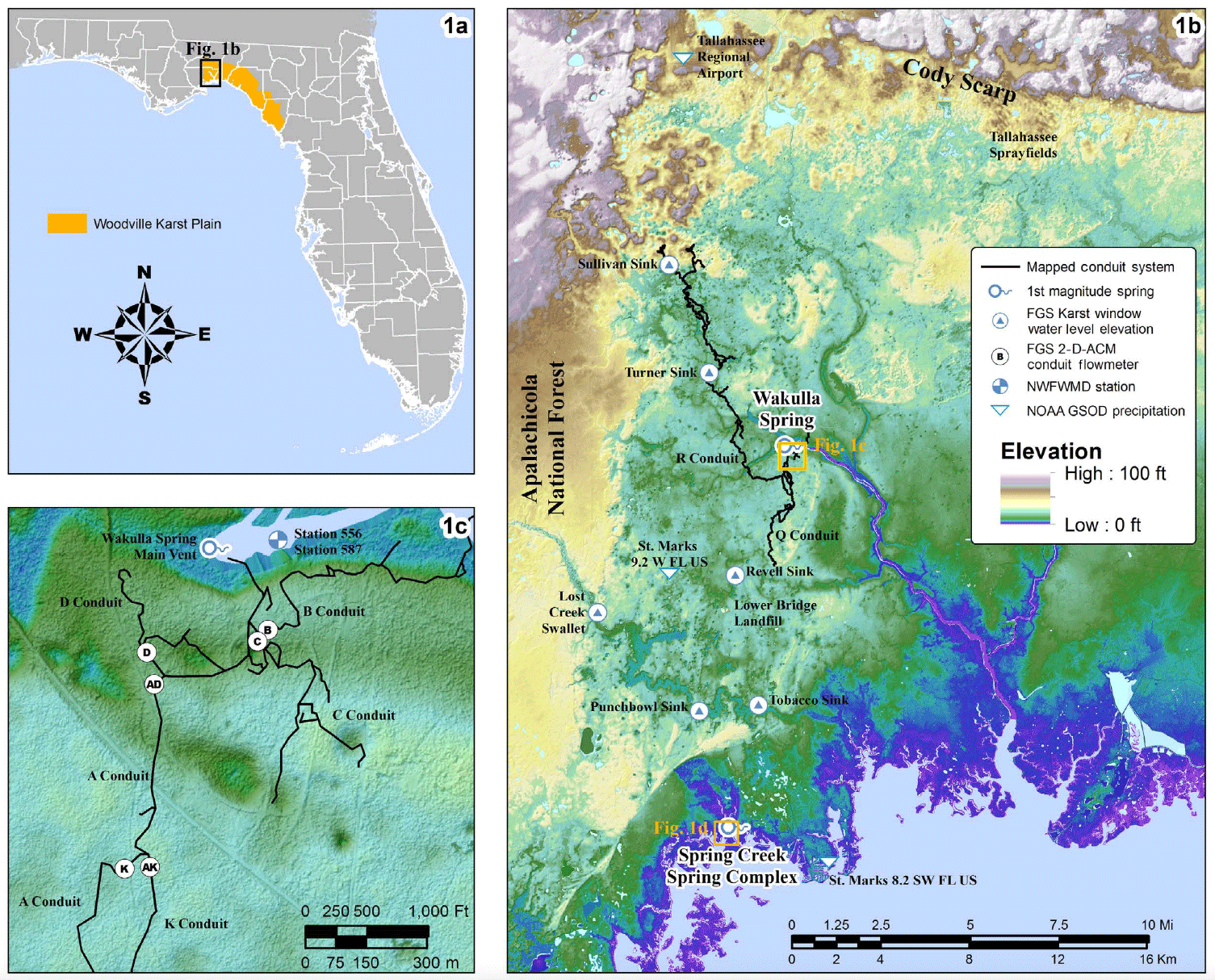
Figure 1(a) Locations of the Woodville Karst Plain (WKP) and the study site. (b) The map of the Woodville Karst Plain showing the locations of features of note in the study. (c) Details of the cave system near Wakulla Spring. Modified from Xu et al. (2016).
In this study, a two-dimensional SEAWAT model is set up to simulate seawater intrusion via the SCS through the major subsurface conduit network in the WKP (Fig. 1). Figure 2 presents the cross section schematic figure in a coastal karst aquifer with a conduit network and a submarine spring opening to the sea. The model spatial domain is not a straight line from the SCS to Wakulla Spring, but it is a cross section along the major conduit pathway of seawater intrusion between the two springs. The conduit geometry in the model is set as 18 km long and 91 m deep, with a height of 10 m in the horizontal part and a width of 50 m in the vertical part.
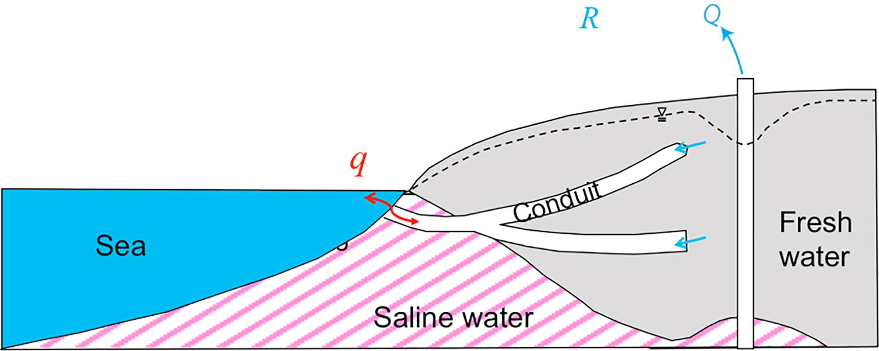
Figure 2Schematic figure of a coastal karst aquifer with conduit networks and a submarine spring opening to the sea in a cross section. Flow direction q would be seaward when sea level drops, pumping rate Q is low, and precipitation recharge R is large; however, reversal flow occurs when sea level rises, pumping rate Q is high, or precipitation recharge R is small.
The two-dimensional model has some limitations on simulating seawater intrusion in the entire aquifer, usually assuming that the quantities are constant parallel to the shoreline. The simulation of seawater intrusion in a perpendicular direction to the cross section as well as three-dimensional flow and transport in the porous matrix are ignored and beyond the scope of this study. However, most SEAWAT models are set up for a two-dimensional cross section with finer resolution vertical discretization. Note that this study only aims to evaluate the parameter sensitivities and simulate seawater intrusion within the vertical cross section of a karst conduit in the aquifer, including flow and transport through the conduit network, the salinity plume in the porous medium, and the exchanges between the two systems. In addition, the two-dimensional assumption is reasonable in the study site since relatively large hydraulic conductivity layers are found at nearly the same depth as the conduit network (Werner, 2001). The permeable layers indicate the possibility of a large extension of the conduit network parallel to the shoreline, although no direct evidence has been found.
3.2 Hydrological parameters
Table 1 presents the hydrological parameter values of the Upper Floridan aquifer (UFA) in the WKP and boundary conditions used in the model. These parameters were calibrated in the regional-scale groundwater flow and solute transport models by Davis et al. (2010) and have been applied in many previous modeling studies (Gallegos et al., 2013; Xu et al., 2015a, b). It should be pointed out that model calibration has not been conducted in this study since the head and salinity observational field data are insufficient, particularly in the conduit, considering the difficulties of monitoring devices' installation in the subsurface conduit. The parameter values in Table 1 are evaluated in the following local sensitivity analysis and then applied in the seawater intrusion scenarios in Sect. 5.
Table 1The symbols and definitions of parameters used in this study, the specified evaluated values in local sensitivity study, and evaluation ranges (the lower and upper constraints) of each parameter in global sensitivity analysis.
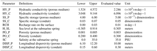
The values of hydrological parameters (hydraulic conductivity, specific storage, and effective porosity) in the conduit are generally greater than those of the surrounding porous medium. Hydraulic conductivity of the porous medium is assigned as 2286 m day−1 and as large as 610 000 m day−1 for the conduit system. Note that even the hydraulic conductivity of the porous medium in the study region is larger than most alluvial aquifers, due to numerous small fractures and relatively large pores existing in the karst aquifer associated with the dissolution of carbonate rocks. Specific storage and effective porosity in the porous medium are assumed to be and 0.003, respectively. Specific storage and effective porosity are 0.005 and 0.300 in the conduit layer, respectively. The longitudinal dispersivity is estimated to be 10 m in the porous medium, but it is assumed to be a very small value (0.3 m) in the conduit because advection is dominating and dispersion is negligible in the solution of transport in the conduit.
3.3 Spatial and temporal discretization
The grid discretization and boundary conditions of the two-dimensional SEAWAT numerical model are shown in Fig. 3, with 140 columns and 37 layers in the cross section. Guo and Langevin (2002) and Werner et al. (2013) pointed out that a fine-resolution vertical grid is required for accurately modeling the density-dependent flow and solute transport. The vertical thickness of each grid cell is set uniformly as 3.048 m (10 ft) in this study, significantly smaller than the large thickness of 152 m in many previous constant-density modeling studies in the WKP, for example, Davis and Katz (2007); Davis et al. (2010); Xu et al. (2015a, b); and Gallegos et al. (2013).
Based on the field scale, the horizontal discretization for each cell is set uniformly at 152 m, except columns no. 22 and no. 139, which are 15.2 m in the vertical conduit network connecting the submarine spring (SCS) and inland spring (Wakulla Spring), respectively. The sizes of spring outlets and the conduit network are based on the observational field data and the calibrated values from the previous modeling studies (Gallegos et al., 2013). For model simplicity, the size of horizontal conduit network is assumed constant in this study. The outlet of vertical conduit system is the submarine spring (SCS) located at the shoreline at column no. 22. The conduit system starts from the submarine spring, descends downward to layer no. 29 (nearly 100 m below sea level), horizontally extends nearly 18 km from column no. 22 to column no. 139, and then rises upward to the top through column no. 139. Seawater intrudes at the SCS on the first layer of column no. 22 and then flows vertically downward into the conduit system. The inland spring is simulated by the DRAIN package as the general head boundary condition in the SEAWAT model. All layers are simulated as confined aquifer since the conduit is fully saturated, which is consistent with the previous numerical models used in Davis et al. (2010) and Xu et al. (2015a, b) in the WKP.
A transient 7-day stress in the SEAWAT model is evaluated throughout this study, except the scenarios of longer simulation time for evaluating seawater intrusion under an extended low rainfall period in Sect. 5.4. The timestep of flow model is set as 0.1 days, and the timestep of transport model is determined by SEAWAT automatically.
3.4 Initial and boundary conditions
The initial condition of head is constant within each layer, set as 0.0 m as the present-day sea level for the cells from the boundary on the left (column no. 1) to the shoreline (column no. 22), and it gradually rises to 1.52 m at inland boundary on the right, determined by the elevation of Wakulla Spring. Note that the head values are written in the input files of the SEAWAT model instead of the equivalent freshwater head. The initial conditions of salinity are assumed to be a constant value of 35.0 PSU, assuming no freshwater dilution at the sea boundary and the leftmost 10 columns. The seawater–freshwater mixing zone is assumed to be from 35 PSU at column no. 11 to 0 PSU at column no. 45, with a gradient of 1.0 PSU per column. Salinity is set uniformly as 0.0 PSU from column no. 46 to the inland boundary on the right, as uncontaminated freshwater before seawater intrudes. Several test cases have been made to confirm that the initial conditions do not significantly affect the modeling results.
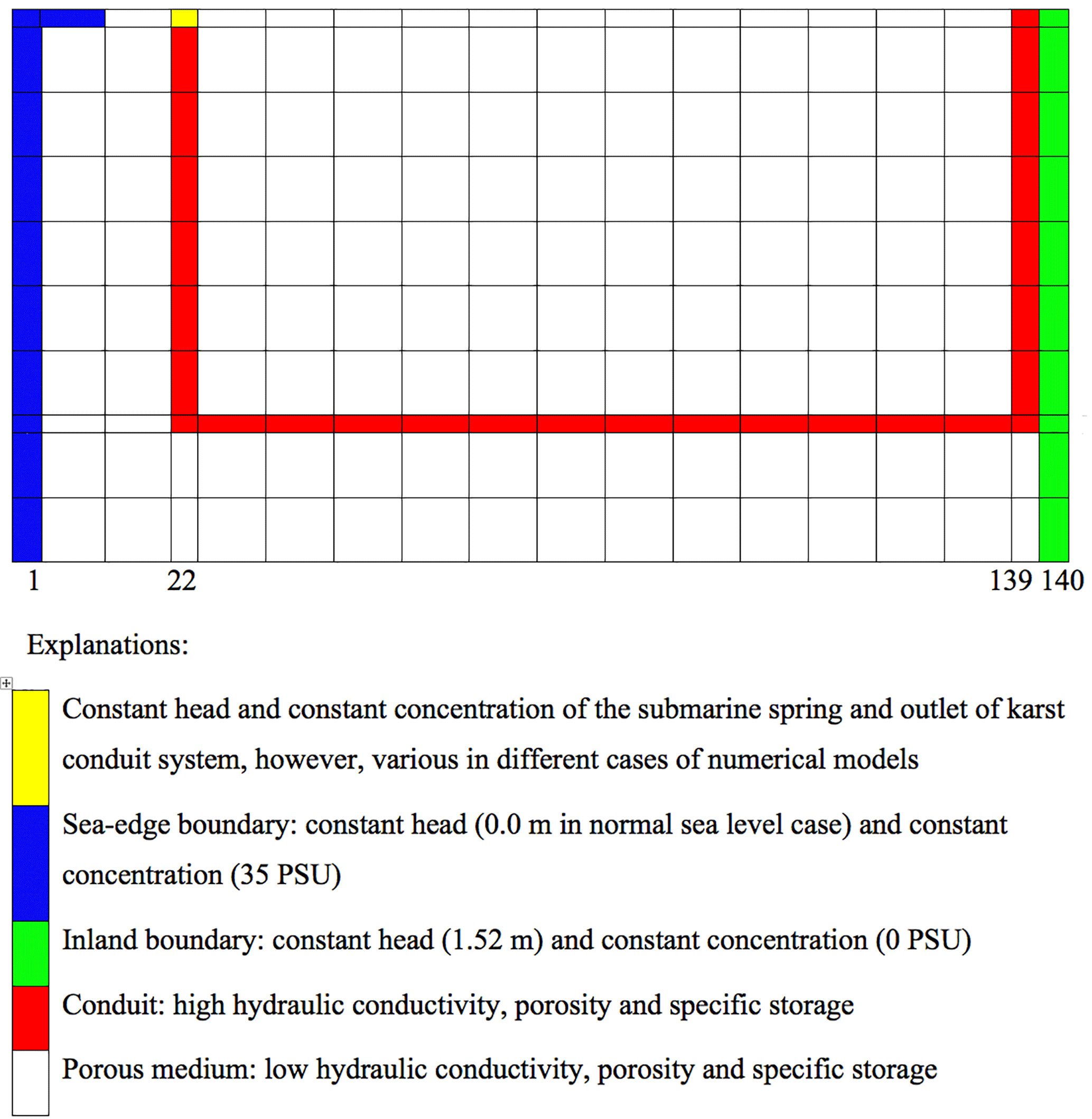
Figure 3Schematic figure of finite difference grid discretization and boundary conditions applied in the SEAWAT model. Every cell represents 10 horizontal cells and 4 vertical cells, except the boundary and conduit layer in color with smaller width. The submarine spring is located at column no. 22, layer no. 1, and the inland spring is located at column no. 139, layer no. 1. The conduit system starts from the top of column no. 22, descends downward to layer no. 29, horizontally extends to column no. 139, and then rises upward to the top through column no. 139.
The boundary conditions are also presented in Fig. 3. The less permeable confining unit of the UFA base is simulated at the bottom of the model domain as the no-flow boundary condition. The constant head and concentration inland boundary condition on the right is 1.5 m as the elevation of inland spring and 0.0 PSU as uncontaminated freshwater. The seawater boundary on the left is 3.38 km away from the shoreline, set as 0.0 m constant head as the present-day sea level and 35.0 PSU constant concentration as seawater without mixing. The boundary conditions of head and salinity at the submarine spring (column no. 22, layer no. 1) are adjusted and evaluated in the scenarios of different sea level, salinity, and rainfall conditions in Sect. 5.
Sensitivity analysis evaluates the uncertainties of salinity and head simulations with respect to eleven parameters, and it helps to understand the effects of variations and interactions of aquifer parameters and boundary conditions on simulations. The symbols and definitions of the eleven parameters are listed in Table 1, as well as the values computed in the local sensitivity analysis and the parameter ranges evaluated in the global sensitivity analysis (Table 1). There are six parameters in the groundwater flow model, including hydraulic conductivity (HY_P and HY_C), specific storage (SS_P and SS_C) of the conduit and of the porous medium, recharge rate (RCH), and the sea level at the submarine spring (H_SL). The other five parameters, including effective porosity (PO_P and PO_C), dispersivity (DISP_P and DISP_C) of the conduit and the porous medium, and the salinity at the submarine spring (SC), are in the solute transport model.
4.1 Local sensitivity analysis
In the local sensitivity analysis, the CSS values of parameters with respect to head and salinity simulations are calculated at several locations along the conduit network and the porous medium, respectively. The CSS values are computed for the parameter values in the maximum seawater intrusion benchmark case in Sect. 5.1, which is developed to quantitatively evaluate the extent of seawater intrusion specifically in the WKP after a 7-day low precipitation period. The parameters to be adjusted and evaluated in the scenarios are also determined based on the local sensitivity result.
Parameter sensitivities are computed at several locations, from column no. 25 to column no. 75 with an interval of five cells along the horizontal conduit (layer no. 29), where column no. 25 is close to the shoreline as fully contaminated by seawater, and column no. 75 is assumed to be the uncontaminated freshwater aquifer. The parameter sensitivities of simulations in a porous medium are evaluated at layer no. 24, 15.2 m, or five layers above the conduit layer, from column no. 25 to column no. 75, with an interval of five cells along the horizontal direction.
4.2 Local sensitivity analysis of simulations in the conduit
Figure 4 shows the arithmetic mean of CSS values computed in the evaluated locations along the conduit layer. The largest CSS value indicates that salinity at the submarine spring (SC) is the most important parameter in both salinity and head simulations. Hydraulic conductivity, specific storage, and effective porosity of the conduit (HY_C, SS_C, and PO_C), as well as the sea level at the submarine spring (H_SL), are also important parameters. Simulations are not sensitive to hydraulic conductivity, specific storage, and effective porosity of the porous medium (HY_P, SS_P, and PO_P), recharge rate (RCH), and dispersivity (DISP_C and DISP_P). Generally speaking, the parameter sensitivities with respect to head simulations are similar and consistent with salinity simulations.
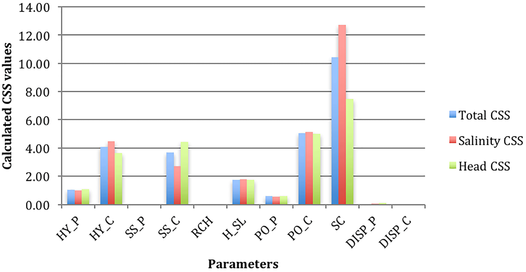
Figure 4The CSS (composite scaled sensitivity) values of all parameters with respect to simulations in the conduit (layer no. 29) in the local sensitivity analysis.
The boundary conditions of the conduit system, including salinity and sea level at the submarine spring (SC and H_SL), are important in modeling seawater intrusion in the WKP. Seawater enters the conduit system at the submarine spring and intrudes landward through the subsurface conduit system. The most important parameter is identified as the salinity at the submarine spring (SC), which affects the equivalent freshwater head in terms of water density at the inlet of the conduit system and affects flow simulation within the conduit system. The salinity at the submarine spring (SC) is determined by freshwater mixing and dilution from the conduit network; in other words, it is controlled by rainfall recharge and freshwater discharge from the aquifer to the sea. In this study, rainfall recharge is represented by salinity at the submarine spring with freshwater dilution instead of the recharge flux on the surface (RCH), which is not an important parameter and not applicable to represent the total rainfall recharge in the two-dimensional SEAWAT model. On the other hand, the sea level at the submarine spring (H_SL) has an intermediate CSS, indicating that it is also important in flow field and salinity transport simulations. However, sea level is not as important as the salinity at the submarine spring (SC). In other words, the extent of seawater intrusion in the conduit is more sensitive to rainfall recharge and freshwater discharge represented by the parameter SC, rather than the sea level and/or tide level variations.
Dispersivity is usually an important parameter in the sensitivity analysis of transport modeling in a porous medium aquifer (Shoemaker et al., 2004). However, the conduit and porous medium dispersivities (DISP_C and DISP_P) are not evaluated as important parameters in the dual-permeability model in this study. Advection dominates in the transport of seawater in the high permeability conduit network, while dispersion is negligible in such a high-velocity flow condition. Moreover, the dispersion solution and dispersivity sensitivities in the conduit are inaccurately calculated when conduit flow becomes turbulent. On the other hand, the numerical dispersion is significantly greater than the physical dispersion in the conduit. The Peclet number can be as great as 2500, far beyond the theoretical criterion (< 4) for solving the advection dispersion transport equation using the finite difference method (Zheng and Bennett, 2002). Dispersivity sensitivities have large uncertainty in this study, indicating that the continuum SEAWAT model is not applicable to accurately compute the salinity dispersion in the conduit. An experiment of deactivating the DSP (dispersion) package in SEAWAT confirms that dispersion is negligible within the conduit network in this study. Instead of the dispersion computed by dispersivity, numerical dispersion is the major reason for the range of mixing interface shown in this study.
The parameters with the six largest CSS values are presented in Fig. 5, with respect to the combination of head and salinity simulations in the evaluated locations along the conduit network, from column no. 25 to column no. 75. The largest CSS values are found at either column no. 50 or no. 55 within the conduit, which matches with the position of the seawater–freshwater mixing zone along the conduit network in the maximum seawater intrusion case (Sect. 5.1). The largest CSS values are found at the mixing zone more than anywhere else for all parameters because head and salinity simulations only change significantly near the mixing zone but remain constant in other locations.
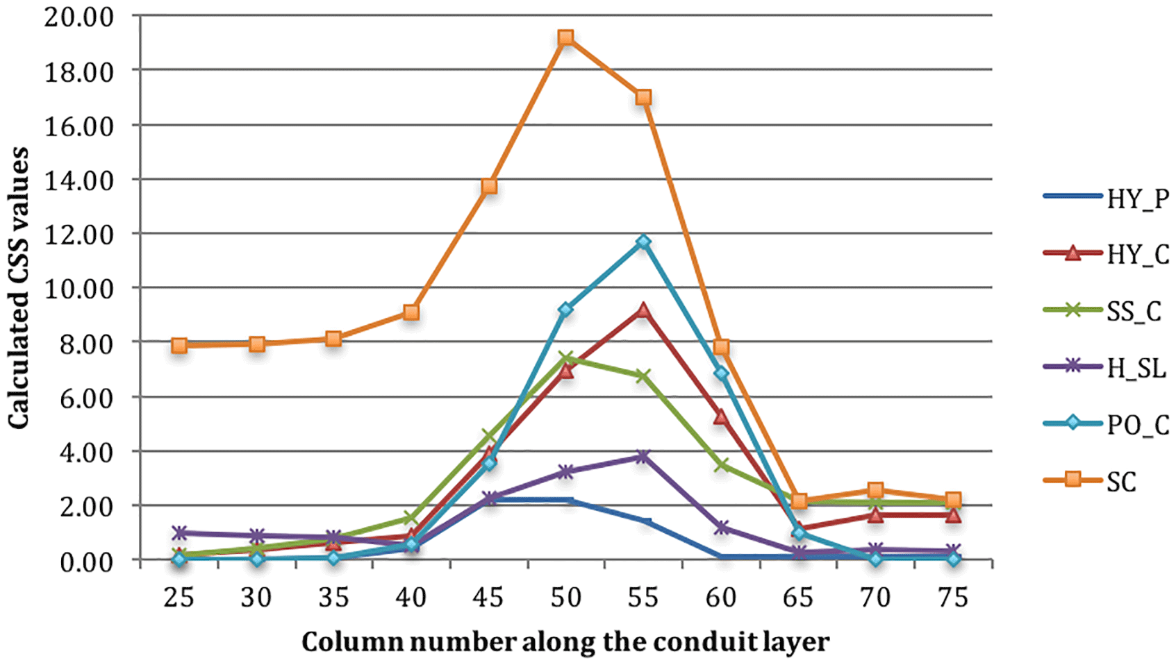
Figure 5The CSS (composite scaled sensitivity) values of selected parameters at different locations along the conduit layer (from column no. 25 to column no. 75) in the local sensitivity analysis.
4.3 Local sensitivity analysis of simulations in the porous medium
Figure 6 shows the arithmetic mean of CSS values computed in the evaluated locations in the porous medium (layer no. 24). The largest CSS value indicates that salinity at the submarine spring (SC) is also the most important parameter with respect to simulations in the porous medium, although it is a boundary condition of the conduit system. However, some parameter sensitivities exhibit different patterns compared to the results of simulations in the conduit. The hydraulic conductivity and effective porosity of both the conduit and porous medium (HY_ C, HY_P, PO_C and PO_P), specific storage of the conduit (SS_C), and dispersivity of the porous medium (DISP_P), have intermediate CSS values. The CSS values at different evaluated locations along the layer of the porous medium are plotted in Fig. 7, except the three unimportant parameters. Similar to the sensitivity analysis of simulations along the conduit, the largest CSS values are found at either column no. 35 or no. 40, which is the mixing zone position in the porous medium in the maximum seawater intrusion case (Sect. 5.1).
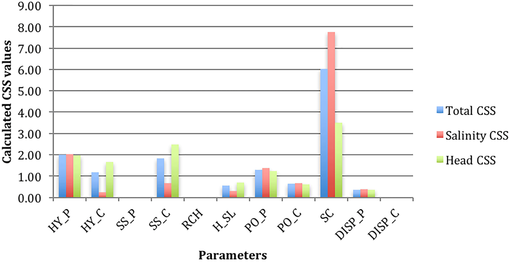
Figure 6The CSS (composite scaled sensitivity) values of all parameters with respect to simulations in the porous medium (layer no. 24) in the local sensitivity analysis.
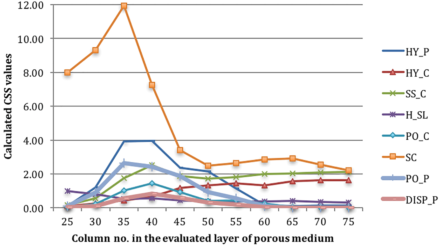
Figure 7The CSS (composite scaled sensitivity) values at different locations in the porous medium (from column no. 25 to column no. 75 at layer no. 24) in the local sensitivity analysis.
The important rules of the boundary condition and hydrological parameters of the conduit system on simulations in the porous medium are highlighted in the local sensitivity analysis. Salinity at the submarine spring (SC) remains the most important parameter and determines the seawater intrusion plume in the porous medium. The conduit parameters, such as hydraulic conductivity, effective porosity, and specific storage (HY_C, PO_C, and SS_C), are also important to the simulations in the porous medium. The CSS values of conduit parameters indicate that groundwater flow and seawater transport through the conduit system have a significant impact on the simulations in the surrounding porous medium. In summary, simulations in the porous medium are sensitive to both the conduit and porous medium parameters, highlighting the interaction between the two domains in simulating seawater intrusion in the dual-permeability WKP coastal karst aquifer. As a result, simulations and observations of salinity and head in the conduits and other karst features have significance for calibrating numerical models and values for understanding seawater intrusion.
4.3.1 Parameter correlations
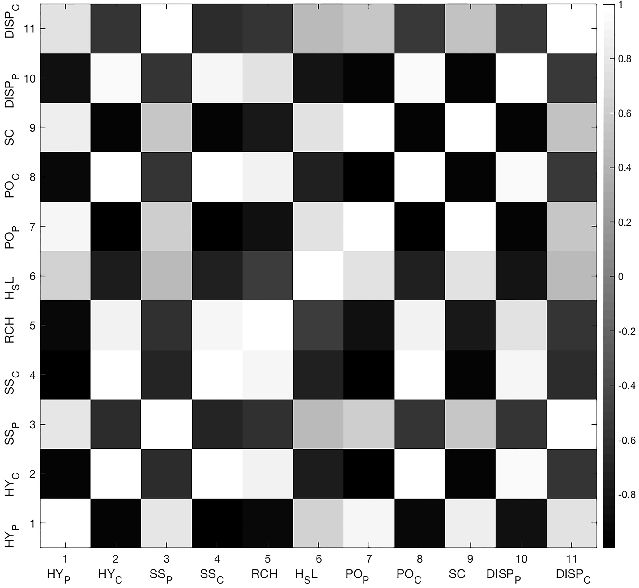
The correlation coefficients and covariance matrix of all parameters are calculated and presented in Fig. 8. The white and black colors represent positive and negative parameter correlations, respectively. Generally speaking, hydrological parameters of the porous medium are positively correlated with the other parameters of the porous medium but negatively correlated with conduit parameters, and vice versa. On the other hand, hydraulic conductivity, specific storage, and porosity have a similar correlation pattern among all evaluated parameters, while the correlation of dispersion is different to others. For example, hydraulic conductivity (HY_P) has a strong positive correlation with specific storage (SS_P) and porosity (PO_P); however, it has a negative correlation with dispersivity (DISP_P). The correlations of conduit parameters exhibit a similar relationship as well. The results can be explained such that a larger hydraulic conductivity would result in higher seepage velocity in either the conduit or the porous medium by Darcy's law; therefore, salt transport from the submarine springs also results in higher salinity in both the conduit porous medium domains. However, larger dispersivity could decrease the peak values of salinity concentration but enlarge contaminant plumes due to stronger dispersion and diffusion.
4.4 Global sensitivity analysis
The local sensitivity analysis analyzes the parameter sensitivities specifically for the seawater intrusion in the WKP, as the maximum seawater intrusion case in Sect. 5.1. However, the local sensitivity result is not representative of the entire parameter range and higher order derivatives of simulations. The global sensitivity analysis is essential to provide a comprehensive understanding of the relationship between simulations and parameters for modeling seawater intrusion in a coastal karst aquifer.
The derivatives of simulations with respect to the selected parameters in Fig. 9 clearly indicate that local sensitivity results are not representative of the entire parameter range. For example, both head and salinity simulations in the conduit are nearly constant in relation to the variation of an unimportant parameter (DISP_P) in the local sensitivity study. However, simulations are nonlinear to salinity at the submarine spring (SC). Parameter SC is identified as the most important parameter in the local sensitivity analysis, partially because the CSS value is computed at the largest derivative value where salinity is 35 PSU.
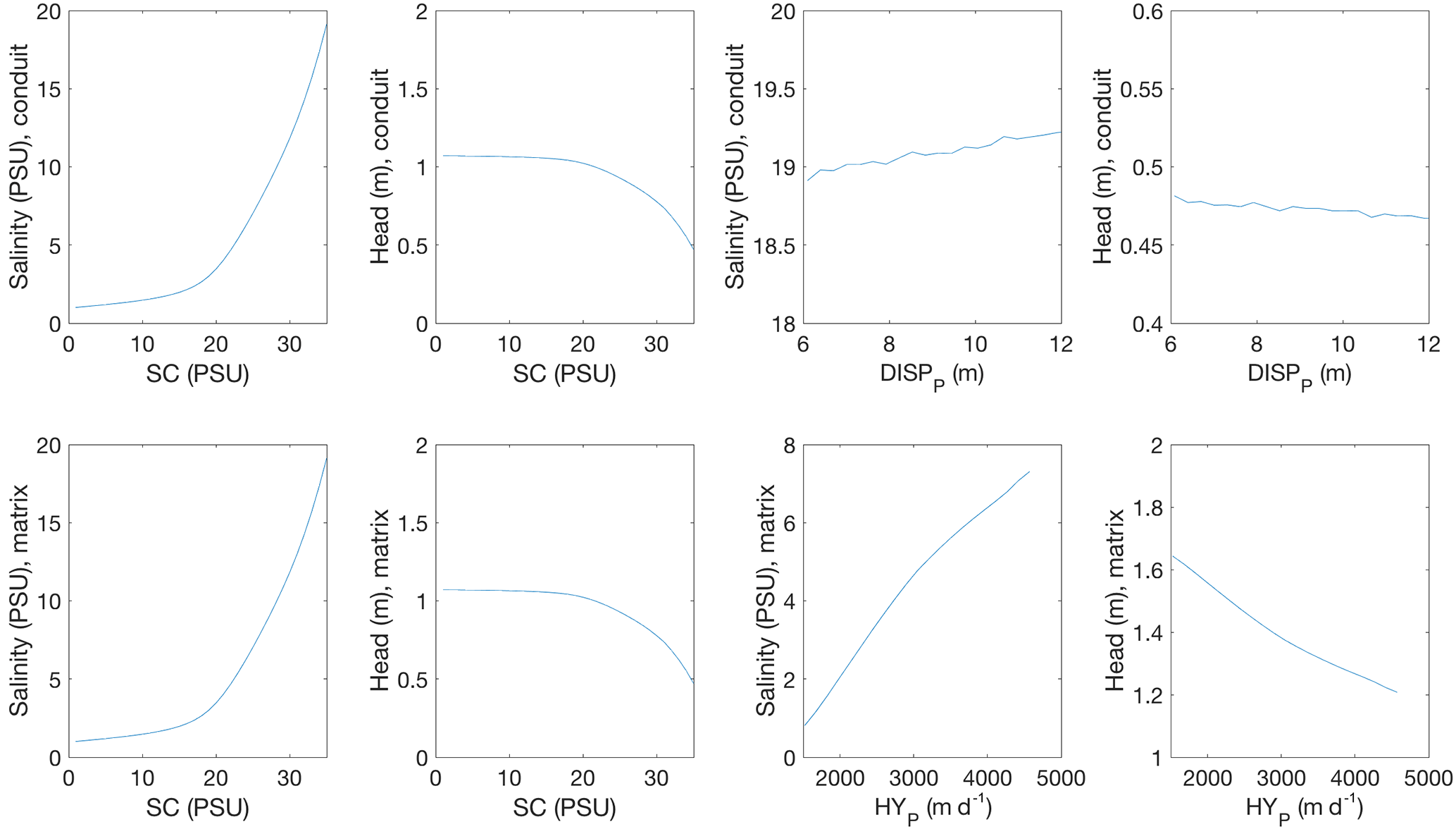
Figure 9The nonlinear relationship between head and salinity simulations with respect to parameters SC, DISP_P, and HY_P. (Note that the scale for each plot is different.)
The locations in the conduit and porous medium systems with the largest CSS values from the local sensitivity analysis are evaluated in the global sensitivity analysis. Parameter sensitivities are computed at the locations with largest CSS values in the previous local sensitivity analysis, specifically, column no. 50, layer no. 29 in the conduit and column no. 35, layer no. 24 in the porous medium, respectively. The trajectory sampling method developed by Saltelli et al. (2004) is introduced in Sect. 2.2 and applied in the global sensitivity analysis, with the recommended choice of p=4 and r=10 by Saltelli et al. (2004).
4.4.1 Global sensitivity analysis of simulations in the conduit
In the global sensitivity analysis, the mean and standard deviation of the EEs for salinity simulation in the conduit (column no. 50, layer no. 29) are presented in Fig. 10a. Consistent with the local sensitivity analysis, the largest mean value of EEs indicates that parameter SC is the most important parameter in salinity simulations. Parameter SC also has the largest standard deviation of the EEs due to the nonlinear relationship between the salinity simulation and parameter SC shown in Fig. 9, in which the derivatives vary with different parameter values. The hydraulic conductivity and effective porosity of the conduit (HY_C and PO_C), as well as sea level (H_SL), are all important to salinity simulation with relatively large mean and standard deviation values of EEs. Generally speaking, the local and global sensitivity study results for salinity simulation in the conduit are similar; however, the standard deviation of EEs provides additional information of parameter sensitivities in the global sensitivity study.
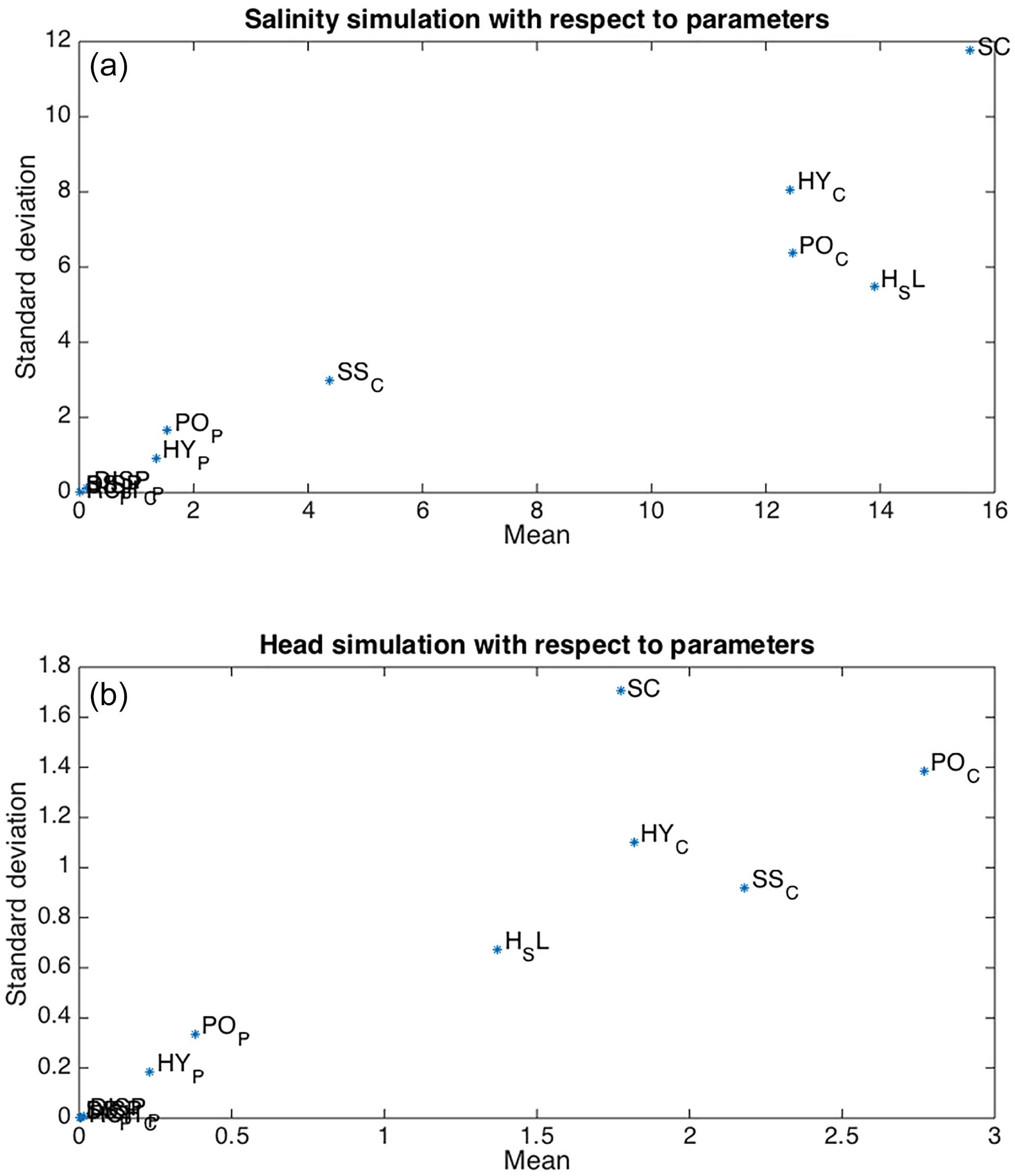
Figure 10Mean and standard deviation of the EEs (elementary effects) of parameters with respect to simulations in the conduit (column no. 50, layer no. 29) in the global sensitivity analysis by the Morris method: (a) salinity simulation (top); (b) head simulation (bottom).
The global sensitivities for head simulations with respect to parameters are more complicated than salinity simulations (Fig. 9b). The mean and standard deviation of EEs for head simulations are smaller than those for salinity simulations, consistent with the conclusion of Shoemaker (2004) that salinity simulations are more effective than head simulations. The two largest mean values of EEs show that the specific storage (SS_C) and effective porosity (PO_C) of the conduit are the two most important parameters. As mentioned in the local sensitivity analysis, parameters in the transport model are also important to the head simulation in a coupled density-dependent flow and transport model. For example, effective porosity is important in head simulation since the solution of salinity transport in turn determines the density and impact flow calculation in the model, particularly in the study of density-dependent seawater intrusion. In addition, head simulations are also sensitive to the boundary conditions of salinity in the transport model since equivalent freshwater head is a function of density in terms of salinity in the coupled variable-density flow and transport model for simulating seawater intrusion. Different from salinity simulation, salinity at the submarine spring (SC) no longer has the largest mean of EEs. However, the standard deviation of EEs for parameter SC is still the largest due to the nonlinear relationship with head simulation shown in Fig. 9.
One of the major findings in the global sensitivity analysis is that the hydraulic conductivity of the conduit (HY_C) has smaller means and standard deviations of EEs than the other two parameters (PO_C and SS_C), and it no longer becomes the most important parameter as shown in the previous local sensitivity analysis. This is different from common knowledge and empirical experience in hydrogeological modeling but is actually reasonable in the karst aquifer with a non-laminar conduit flow. In the SEAWAT model, the Darcy equation is used to calculate the flow velocity in the whole model domain including the conduit system; however, it is only accurate for laminar seepage flow in the porous medium. Groundwater flow is usually non-laminar and even turbulent in the conduit system when the conduit flow rate is nonlinear to the head gradient and hydraulic conductivity. The simulation of conduit flow is beyond the applicability of the Darcy equation in the SEAWAT model, with relatively large error and uncertainty in the relationship between hydraulic conductivity and head simulation. Then, the uncertainty of hydraulic conductivity sensitivities can be too large and difficult to be accurately measured.
4.4.2 Global sensitivity analysis of simulations in the porous medium
The hydraulic conductivity of the porous medium (HY_P) and salinity at the submarine spring (SC) are identified as the two most important parameters for salinity simulations in the porous medium (Fig. 11a). Compared to parameter HY_P, parameter SC has a much larger CSS value at 35.0 PSU with the largest derivative in the local sensitivity analysis (Fig. 6) and also a larger standard deviation of EEs in the global sensitivity analysis. Local sensitivity analysis overestimates the sensitivity of parameter SC within the range, and global sensitivity analysis provides a more comprehensive understanding of the physical meaning of parameter SC, for example, variability of rainfall recharge and freshwater discharge. As the boundary condition of the conduit system, salinity at the submarine spring (SC) determines the equivalent freshwater head at the inlet of seawater intrusion and affects simulations in the conduit and also the surrounding porous medium via exchanges between the two systems. The global sensitivity results highlight the significance of conduit and porous medium interactions in a dual-permeability aquifer. Similar to salinity at the submarine spring (SC), dynamic interactions between the conduit and the porous medium in this study are clearly shown in the relatively large mean of EEs for sea level (H_SL), effective porosity, and specific storage of the conduit (PO_C and SS_C). Effective porosity is important for head simulations in this study since the density-dependent flow and transport models are coupled for simulating seawater intrusion.
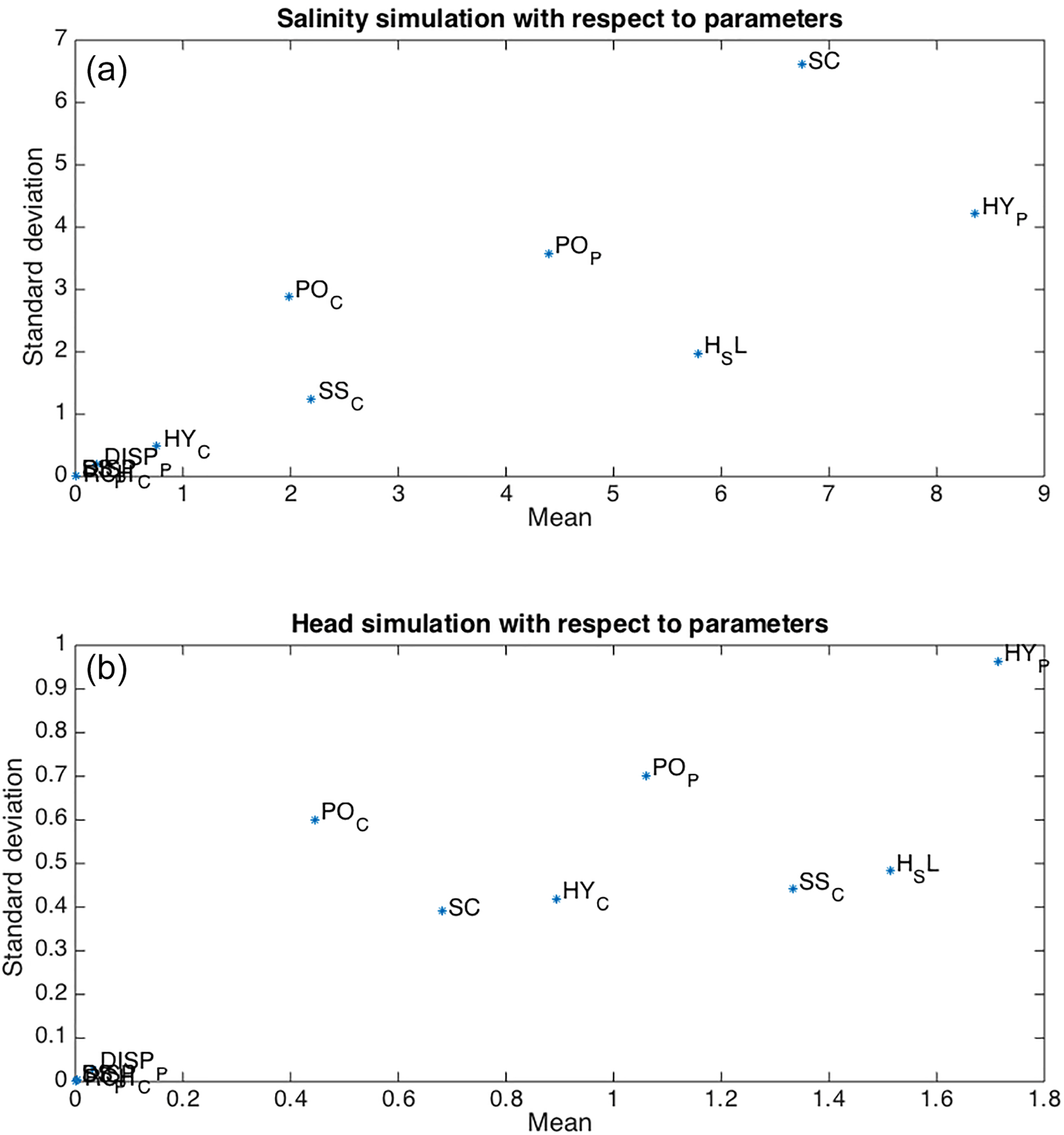
Figure 11Mean and standard deviation of the EEs (elementary effects) of parameters with respect to simulations in the porous medium (column no. 35, layer no. 24) in the global sensitivity analysis by the Morris method: (a) salinity simulation (top); (b) head simulation (bottom).
On the other hand, parameter sensitivities for simulations in the porous medium are different to the sensitivities for simulations in the conduit. The porous medium hydraulic conductivity (HY_P) is an important term in the flow equation for solving head and advective velocity for the transport equation (Fig. 11b), similar to most sensitivity results of hydrological modeling for flow in a porous medium. For the simulations in the conduit, effective porosity and specific storage of the conduit (PO_C and SS_C) are more important than hydraulic conductivity (HY_C) because of the large uncertainty in conduit flow computation by Darcy's equation in the continuum SEAWAT model.
In this section, the extents of seawater intrusion are quantitatively measured and evaluated under different scenarios of boundary conditions, which are identified as the important parameters in the local sensitivity analysis. In each scenario, only one parameter is adjusted and others are constant, as in the maximum seawater intrusion benchmark case in Sect. 5.1.
5.1 The maximum seawater intrusion benchmark case
The local sensitivity analysis computes the sensitivities of parameter values in the maximum seawater intrusion benchmark case, which assumes the head and salinity boundary conditions are 0.0 m as the present-day sea level, and 35.0 PSU as seawater without dilution at the conduit system outlet, respectively. Salinity and sea level at the submarine spring (SC and H_SL) are identified as two important parameters and then adjusted in the following two scenarios. In this case, the longest distance of seawater intrusion is simulated with the assumption that freshwater recharge is negligible, and the outlet of conduit system is filled with undiluted seawater. Figure 12 presents the simulated salinity and head profile in the cross section after a 7-day simulation.
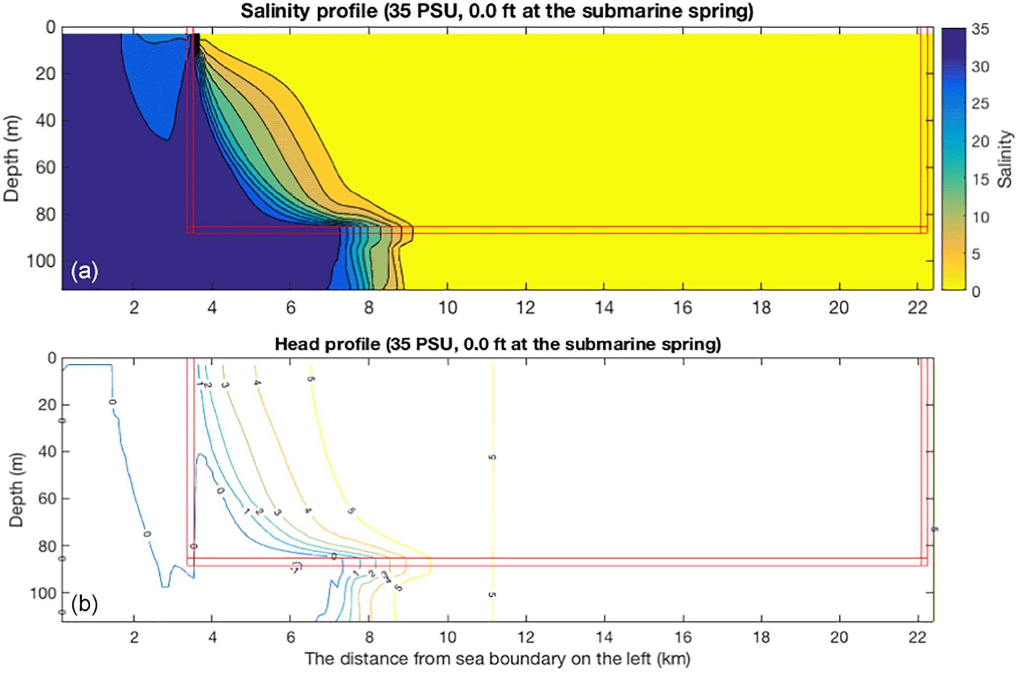
Figure 12Salinity (a) and head (b) simulations of the maximum seawater intrusion benchmark case (35 PSU, 0.0 m at the submarine spring).
According to the Ghyben–Herzberg relationship, landward seawater intrusion is on the bottom of the aquifer beneath the seaward freshwater on the top. The equivalent freshwater head at the submarine spring is calculated as 2.29 m when salinity is 35.0 PSU at the submarine spring, and undiluted seawater is filled within the 91 m deep submarine cave and conduit network. The equivalent freshwater head at the submarine spring is higher than the 1.52 m constant head at the inland spring, diverts the hydraulic gradient landward, and causes seawater to intrude into the aquifer. Seawater intrudes further landward through the highly permeable conduit network; it also contaminates the surrounding porous medium via exchange on the conduit wall. The seawater–freshwater mixing zone in the deep porous medium beneath the conduit is only slightly behind the seawater front in the conduit because high-density saline water easily descends from the conduit and flows downward. The area with relatively smaller salinity to the left of the vertical conduit network nearshore is due to the freshwater discharge dilution from the aquifer to the sea since the equivalent freshwater head is only 2.29 m at the submarine spring but remains 0 m in other areas. The mixing zone position in the conduit, defined as the location with a salinity of 5.0 PSU, is measured at nearly 5.80 km landward from the shoreline. The width of mixing interfaces, defined as the distance between the locations with a salinity of 1.0 and 25.0 PSU, is roughly the same as seven grid cells or 1.13 km in both the conduit and porous medium.
5.2 Salinity variation at the submarine spring (SC)
Sensitivity analysis indicates that the salinity at the submarine spring (SC) is generally the most important parameter for simulations in both the conduit and the porous medium. Salinity at the submarine spring is diluted by a large amount of rainfall recharge and freshwater discharge after a significant precipitation event, but it remains highly saline after an extended low rainfall period, as shown in the maximum seawater intrusion benchmark case in Sect. 5.1. The equivalent freshwater head at the submarine spring is 2.29 m when salinity is 35.0 PSU, and it proportionally decreases to 0.0 m when salinity is 0.0 PSU and freshwater is filled within the conduit system. The impact of freshwater recharge on seawater intrusion is evaluated in four scenarios with salinity levels of 0.0, 10.0, 20.0, and 30.0 PSU at the submarine spring (Fig. 13). The mixing zone in both the conduit and porous medium is measured at 4.0 (4.5) km away from the shoreline in the case of a salinity of 10.0 (20.0) PSU at the submarine spring. Compared to the maximum seawater intrusion benchmark case, rainfall recharge and freshwater discharge dilute seawater intrusion and move the interface significantly seaward. The mixing zone is very close to the shoreline when salinity is 0.0 PSU at the submarine spring and seawater intrusion is blocked by a large amount of freshwater dilution. The shape of the mixing interface is similar to the maximum seawater intrusion benchmark, but the width of the mixing interface is wider due to the slower advective flow with a smaller or even reversed hydraulic gradient from the aquifer to the sea. In the scenarios of freshwater dilution, the solution of dispersion becomes more accurate and important in salinity transport with slower groundwater seepage flow. Generally speaking, a heavy rainfall event dilutes the intruded seawater and moves the mixing interface seaward.
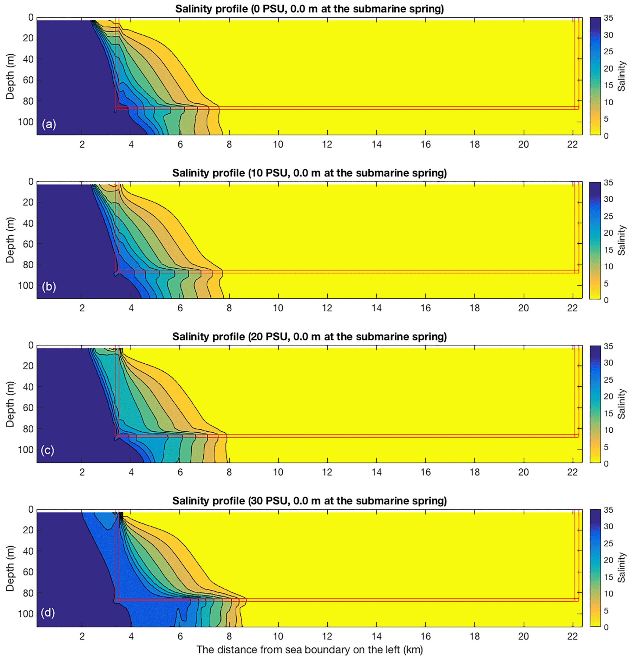
Figure 13Salinity simulation of seawater intrusion with various salinities at the submarine spring, indicating different rainfall recharge and freshwater discharge conditions: (a) 0.0 PSU, 0.0 m at the submarine spring; (b) 10.0 PSU, 0.0 m at the submarine spring; (c) 20.0 PSU, 0.0 m at the submarine spring; (d) 30.0 PSU, 0.0 m at the submarine spring (from top to bottom).
5.3 Sea level variation at the submarine spring (H_SL)
In addition to salinity, sensitivity analysis indicates that sea level at the submarine spring is also an important parameter. IPCC (2007) predicted an approximation of 1.0 m sea level rise by the end of 21st century, which has significant impacts on seawater intrusion in a coastal karst aquifer. The extents of seawater intrusion in the conduit and porous medium under 0.91 and 1.82 m sea level rise conditions are quantitatively evaluated in this study (Fig. 14). Salinity at the submarine spring remains 35.0 PSU, but the head at the submarine spring increases to simulate rising sea level. The simulated salinity profiles show that the width and shape of the mixing zone are similar to the results in the maximum seawater intrusion benchmark. However, the mixing zone is intruded landward along the conduit to almost 7.08 km from the shoreline with 0.91 m sea level rise, which is 1.28 km further inland than the simulation under present-day sea level. In the other extreme case of 1.82 m sea level rise, seawater intrudes an additional 0.97 km further inland along the conduit than the simulated result with 0.91 m sea level rise, or 2.25 km further landward than the simulation under present-day sea level. Compared to the porous alluvial aquifer, seawater intrudes further landward through the conduit network in the a dual-permeability karst aquifer under sea level rise. This scenario confirms the concerns of severe seawater intrusion in the coastal karst aquifer under sea level rise, and it also highlights the value of the conduit system as the major pathway for long-distance seawater intrusion. In addition, sea level rise might have great impacts on the regional flow field and hydrological conditions in a coastal aquifer. Davis and Verdi (2014) reported an increasing groundwater discharge at the inland Wakulla Spring in the WKP associated with the rising sea level in the past decades. The relationship between spring discharge and sea level was quantitatively simulated by a CFPv2 numerical model in Xu et al. (2015b); however, this is beyond the scope of this study.
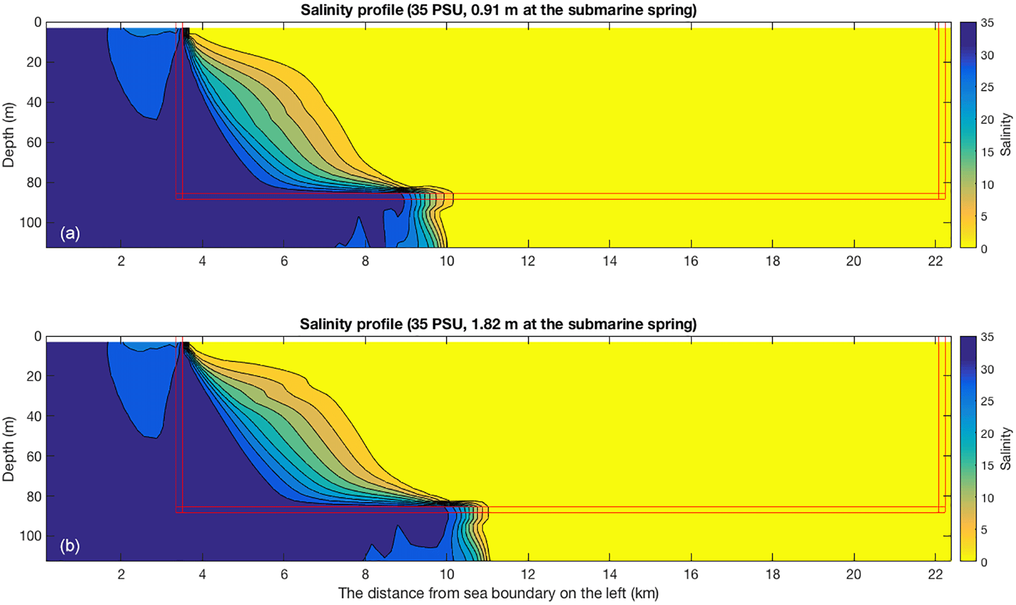
Figure 14Salinity simulation of seawater intrusion with various sea level conditions: (a) 35.0 PSU, 0.91 m at the submarine spring; (b) 35.0 PSU, 1.82 m at the submarine spring (from top to bottom).
5.4 Extended low rainfall period
The elapsed time in simulations is set at constant in the sensitivity analysis and the previous scenarios for consistent comparison purposes. However, extents of seawater intrusion under scenarios of extended low rainfall periods are presented in Fig. 15, with the extended simulated time of 14, 21, and 28 days. The boundary conditions of salinity and sea level at the submarine spring remain 35.0 PSU and 0.0 m, respectively, as the maximum seawater intrusion benchmark.
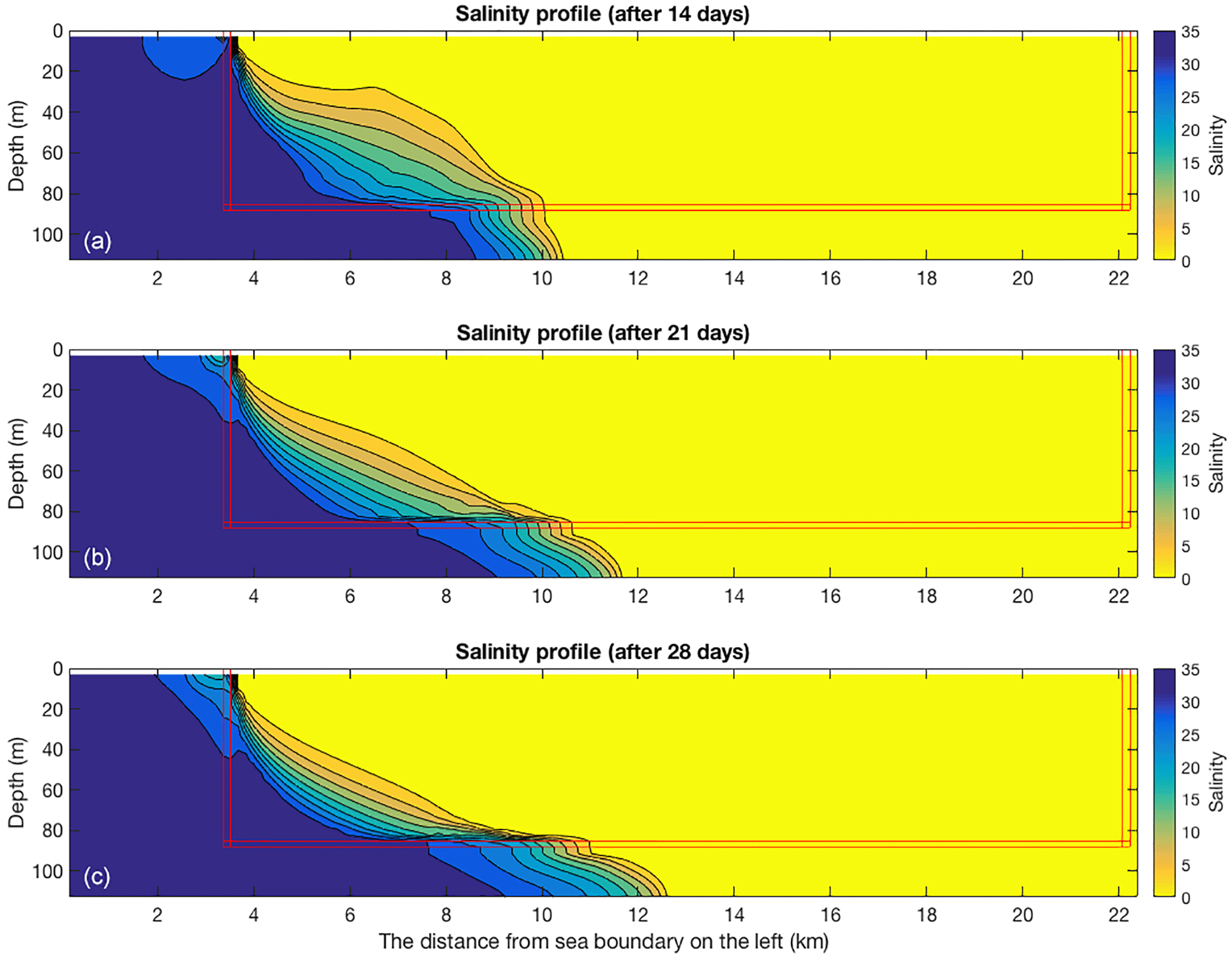
Figure 15Salinity simulation of the maximum seawater intrusion benchmark case (35 PSU, 0.0 m at the submarine spring) with extended simulation time during a low rainfall period: (a) 14-day simulation period; (b) 21-day simulation period; (c) 28-day simulation period (from top to bottom).
Seawater persistently intrudes through both the conduit and the porous medium domains during the extended low rainfall period since the 2.29 m equivalent freshwater head at the submarine spring is higher than the inland freshwater boundary. Compared to the maximum seawater intrusion benchmark with a stress period of 7-day elapsed time in the simulation, the mixing zone position moves an additional 1.29 km landward in the conduit and the surrounding porous medium in the 14-day simulation. In the predictions of 21-day (28-day) extended low rainfall period, the mixing zone finally arrives at 7.56 (7.89) km from the shoreline. Above all, seawater intrudes further inland through the conduit network during an extended low rainfall period, contaminates fresh groundwater resources in the aquifer, and becomes an environmental issue in coastal regions.
In this study, a two-dimensional SEAWAT model is developed to study seawater intrusion in a dual-permeability coastal karst aquifer with a conduit network. Local and global sensitivity analyses are used to evaluate the parameter sensitivities and then understand the roles of hydrogeology conditions and karst features in seawater intrusion. Some major conclusions from the sensitivity analysis are summarized here.
-
Compared to the one specified parameter value computed in the local sensitivity analysis, the global sensitivity analysis is important to accurately estimate the parameter sensitivities in wide ranges, due to the parameter interactions and nonlinear relationship between simulations and parameters shown in Fig. 9. Different from constant-density karst studies, head simulations are sensitive to the boundary conditions and parameters of transport equation since the solution of salinity in terms of density determines the equivalent freshwater head in the coupled density-dependent flow and transport SEAWAT model.
-
Overall, salinity at the submarine spring (SC) is the most important parameter. The boundary conditions and hydrological parameters of the conduit system are not only important to the simulations in the conduit, but also to the porous medium via exchanges between the two systems. The submarine spring and conduit system are the major entrance and pathway, respectively, for seawater intrusion in the coastal karst aquifer. Sensitivity analysis indicates that the simulations of seawater intrusion through the conduit are important for understanding the hydrogeological processes in the dual-permeability karst aquifer, and field observational data, particularly within the conduit system, are essential for the model calibration.
-
Different from the previous studies in Shoemaker (2004), dispersivity is no longer an important parameter for simulations in the conduit. Advection is dominant but dispersion is negligible in salinity transport under the conditions of turbulent flow in the conduit and also the relatively fast seepage flow in the surrounding porous medium. The interaction between the conduit and the porous medium significantly changes the flow field and affects the applicability of the transport model. In the simulated salinity profile, mixing process is mostly due to numerical dispersion instead of the solution of dispersion equation since the Peclet number is extremely large in the domain and beyond the criteria of solving transport equation by finite difference method.
-
Hydraulic conductivity is no longer an important parameter for simulations in the conduit. Conduit flow is usually non-laminar and beyond the applicability range of the Darcy equation used in the SEAWAT model, which assumes a linear relationship between specific discharge and head gradient. Therefore, the uncertainty and sensitivity of conduit permeability is difficult to be accurately evaluated by hydraulic conductivity in the continuum model.
The extents of seawater intrusion and width of mixing interface are quantitatively measured with a different salinity and sea level at the submarine spring, which are identified as important parameters in the sensitivity study. In the maximum seawater intrusion benchmark case with salinity and head as 35.0 PSU and 0.0 m at the submarine spring, respectively, the mixing zone in the conduit moves to 5.80 km from the shoreline with a width of 1.13 km after a 7-day low rainfall period. Rainfall and regional recharges dilute the salinity at the submarine spring (SC) and significantly shift the mixing zone position seaward to 4.0 (4.5) km away from the shoreline with a salinity of 10.0 (20.0) PSU. Compared to the benchmark, seawater intrudes an additional 1.29 (2.25) km further landward along the conduit under 0.91 (1.82) m sea level rise at the submarine spring (H_SL). In addition, the impacts of extended low rainfall on seawater intrusion through the conduit network are also quantitatively assessed with a longer elapsed time in simulations. The mixing zone moves to 7.56 (7.89) km from the shoreline after a 21 (28)-day low precipitation period.
In summary, the modeling and field observations of the karst features, including the subsurface conduit network, the submarine spring, and karst windows, are critical for understanding seawater intrusion in a coastal karst aquifer and important for model calibration. The discrete-continuum density-dependent flow and transport model, for example, the VDFST-CFP in Xu and Hu (2017), is important to accurately simulate seawater intrusion and assess parameter sensitivities in the coastal karst aquifer with conduit networks. Advanced numerical methods and/or high-performance computing are expected to solve the issue of Peclet number limitation and reduce the uncertainty of the dispersion solution with a finer spatial resolution in this study.
The SEAWAT model, UCODE files, and global sensitivity codes can be obtained by contacting the corresponding author Zexuan Xu (xuzexuan@gmail.com).
The authors declare that they have no conflict of interest.
The authors would like to thank associate editor Mauro Giudici and two
anonymous reviewers for their constructive comments and suggestions in the
review process. Bill X. Hu is partially supported by the National Natural
Science Foundation of China (grant no.
41530316).
Edited by: Mauro Giudici
Reviewed by: two anonymous referees
Bear, J.: Seawater intrusion in coastal aquifers, Springer Science & Business Media, 1999.
Calvache, M. and Pulido-Bosch, A.: Effects of geology and human activity on the dynamics of salt-water intrusion in three coastal aquifers in southern Spain, Environ. Geol., 30, 215–223, 1997.
Chang, Y., Wu, J., Jiang, G., and Kang, Z.: Identification of the dominant hydrological process and appropriate model structure of a karst catchment through stepwise simplification of a complex conceptual model, J. Hydrol., 548, 75–87, 2017.
Chen, Z., Hartmann, A., and Goldscheider, N.: A new approach to evaluate spatiotemporal dynamics of controlling parameters in distributed environmental models, Environ. Model. Softw., 87, 1–16, 2017.
Custodio, E.: Salt-fresh water interrelationships under natural conditions, Groundwater Problems in Coastal Areas, UNESCO Studies and Reports in Hydrology, 45, 14–96, 1987.
Davis, J. H.: Hydraulic investigation and simulation of ground-water flow in the Upper Floridan aquifer of north central Florida and southwestern Georgia and delineation of contributing areas for selected City of Tallahassee, Florida, Water-Supply Wells, U.S. Geological Survey, Tallahassee, Florida, 95-4296, 55 pp., 1996.
Davis, J. H. and Katz, B. G.: Hydrogeologic investigation, water chemistry analysis, and model delineation of contributing areas for City of Tallahassee public-supply wells, Tallahassee, Florida, Geological Survey (US)2328-0328, 2007.
Davis, J. H. and Verdi, R.: Groundwater Flow Cycling Between a Submarine Spring and an Inland Fresh Water Spring, Groundwater, 52, 705–716, 2014.
Davis, J. H., Katz, B. G., and Griffin, D. W.: Nitrate-N movement in groundwater from the land application of treated municipal wastewater and other sources in the Wakulla Springs Springshed, Leon and Wakulla counties, Florida, 1966–2018, US Geol Surv Sci Invest Rep, 5099, 90 pp., 2010.
Diersch, H.: FEFLOW reference manual, Institute for Water Resources Planning and Systems Research Ltd, 278, 2002.
Essink, G., Van Baaren, E., and De Louw, P.: Effects of climate change on coastal groundwater systems: a modeling study in the Netherlands, Water Resour. Res., 46, W00F04, https://doi.org/10.1029/2009WR008719, 2010.
Fleury, P., Bakalowicz, M., and de Marsily, G.: Submarine springs and coastal karst aquifers: a review, J. Hydrol., 339, 79–92, 2007.
Gallegos, J. J., Hu, B. X., and Davis, H.: Simulating flow in karst aquifers at laboratory and sub-regional scales using MODFLOW-CFP, Hydrogeol. J., 21, 1749–1760, 2013.
Guo, W. and Langevin, C.: User's guide to SEWAT: a computer program for simulation of three-dimensional variable-density ground-water flow, Water Resources Investigations Report. United States Geological Survey, 2002.
Hartmann, A., Gleeson, T., Rosolem, R., Pianosi, F., Wada, Y., and Wagener, T.: A large-scale simulation model to assess karstic groundwater recharge over Europe and the Mediterranean, Geosci. Model Dev., 8, 1729–1746, https://doi.org/10.5194/gmd-8-1729-2015, 2015.
Hill, M. C. and Tiedeman, C. R.: Effective groundwater model calibration: with analysis of data, sensitivities, predictions, and uncertainty, John Wiley & Sons, 2006.
IPCC: Contribution of Working Groups I, II and III to the Fourth Assessment Report of the Intergovernmental Panel on Climate Change, Geneva, Switzerland, 104 pp., 2007.
Kaufmann, G. and Braun, J.: Karst aquifer evolution in fractured, porous rocks, Water Resour. Res., 36, 1381–1391, 2000.
Kernagis, D. N., McKinlay, C., and Kincaid, T. R.: Dive Logistics of the Turner to Wakulla Cave Traverse, 2008.
Kincaid, T. R. and Werner, C. L.: Conduit Flow Paths and Conduit/Matrix Interactions Defined by Quantitative Groundwater Tracing in the Floridan Aquifer, Sinkholes and the Engineering and Environmental Impacts of Karst: Proceedings of the Eleventh Multidisciplinary Conference, Am. Soc. of Civ. Eng. Geotech. Spec. Publ., 288–302, 2008.
Langevin, C. D., Shoemaker, W. B., and Guo, W.: MODFLOW-2000, the US Geological Survey Modular Ground-Water Model–Documentation of the SEAWAT-2000 Version with the Variable-Density Flow Process (VDF) and the Integrated MT3DMS Transport Process (IMT), US Department of the Interior, US Geological Survey, 2003.
Martin, J. B. and Dean, R. W.: Exchange of water between conduits and matrix in the Floridan aquifer, Chem. Geol., 179, 145–165, 2001.
Martin, J. B., Gulley, J., and Spellman, P.: Tidal pumping of water between Bahamian blue holes, aquifers, and the ocean, J. Hydrol., 416, 28–38, 2012.
Moore, W. S. and Wilson, A. M.: Advective flow through the upper continental shelf driven by storms, buoyancy, and submarine groundwater discharge, Earth Planet. Sc. Lett., 235, 564–576, 2005.
Morris, M. D.: Factorial sampling plans for preliminary computational experiments, Technometrics, 33, 161–174, 1991.
Poeter, E. P. and Hill, M. C.: Documentation of UCODE, a computer code for universal inverse modeling, DIANE Publishing, 1998.
Reimann, T., Liedl, R., Giese, M., Geyer, T., Maréchal, J.-C., Dörfliger, N., Bauer, S., and Birk, S.: Addition and Enhancement of Flow and Transport processes to the MODFLOW-2005 Conduit Flow Process, 2013 NGWA Summit – The National and International Conference on Groundwater, 2013.
Reimann, T., Giese, M., Geyer, T., Liedl, R., Maréchal, J. C., and Shoemaker, W. B.: Representation of water abstraction from a karst conduit with numerical discrete-continuum models, Hydrol. Earth Syst. Sci., 18, 227–241, https://doi.org/10.5194/hess-18-227-2014, 2014.
Saltelli, A., Tarantola, S., Campolongo, F., and Ratto, M.: Sensitivity analysis in practice: a guide to assessing scientific models, John Wiley & Sons, 2004.
Scanlon, B. R., Mace, R. E., Barrett, M. E., and Smith, B.: Can we simulate regional groundwater flow in a karst system using equivalent porous media models? Case study, Barton Springs Edwards aquifer, USA, J. Hydrol., 276, 137–158, 2003.
Shoemaker, W. B.: Important observations and parameters for a salt water intrusion model, Ground Water, 42, 829–840, 2004.
Shoemaker, W. B., Kuniansky, E. L., Birk, S., Bauer, S., and Swain, E. D.: Documentation of a conduit flow process (CFP) for MODFLOW-2005, U.S. Geological Survey Techniques and Methods, Book 6, chap. A24, 50 pp., 2008.
Voss, C. I. and Provost, A. M.: SUTRA, US Geological Survey Water Resources Investigation Reports, 84-4369, 1984.
Voss, C. I. and Souza, W. R.: Variable density flow and solute transport simulation of regional aquifers containing a narrow freshwater–saltwater transition zone, Water Resour. Res., 23, 1851–1866, 1987.
Werner, A. D. and Simmons, C. T.: Impact of sea–level rise on sea water intrusion in coastal aquifers, Groundwater, 47, 197–204, 2009.
Werner, A. D., Bakker, M., Post, V. E., Vandenbohede, A., Lu, C., Ataie-Ashtiani, B., Simmons, C. T., and Barry, D. A.: Seawater intrusion processes, investigation and management: recent advances and future challenges, Adv. Water Resour., 51, 3–26, 2013.
Werner, C. L.: Preferential flow paths in soluble porous media and conduit system development in carbonates of the Woodville Karst Plain, Florida, Master of Science, Department of Earth, Ocean and Atmosphere Science, Florida State University, Tallahassee, FL, 2001.
Wilson, A. M., Moore, W. S., Joye, S. B., Anderson, J. L., and Schutte, C. A.: Storm-driven groundwater flow in a salt marsh, Water Resour. Res., 47, W02535, https://doi.org/10.1029/2010WR009496, 2011.
Xu, Z. and Hu, B. X.: Development of a discrete-continuum VDFST-CFP numerical model for simulating seawater intrusion to a coastal karst aquifer with a conduit system, Water Resour. Res., 53, 688–711, https://doi.org/10.1002/2016WR018758, 2017.
Xu, Z., Hu, B. X., Davis, H., and Cao, J.: Simulating long term nitrate-N contamination processes in the Woodville Karst Plain using CFPv2 with UMT3D, J. Hydrol., 524, 72–88, 2015a.
Xu, Z., Hu, B. X., Davis, H., and Kish, S.: Numerical study of groundwater flow cycling controlled by seawater/freshwater interaction in a coastal karst aquifer through conduit network using CFPv2, J. Contam. Hydrol., 182, 131–145, 2015b.
Xu, Z., Bassett, S. W., Hu, B., and Dyer, S. B.: Long distance seawater intrusion through a karst conduit network in the Woodville Karst Plain, Florida, Scientific Reports, 6, 2016.
Zheng, C. and Bennett, G. D.: Applied contaminant transport modeling, Wiley-Interscience New York, 2002.