the Creative Commons Attribution 4.0 License.
the Creative Commons Attribution 4.0 License.
 | 20 Apr 2018
Analytical flow duration curves for summer streamflow in Switzerland
Ana Clara Santos
Maria Manuela Portela
Andrea Rinaldo
Bettina Schaefli
This paper proposes a systematic assessment of the performance of an analytical modeling framework for streamflow probability distributions for a set of 25 Swiss catchments. These catchments show a wide range of hydroclimatic regimes, including namely snow-influenced streamflows. The model parameters are calculated from a spatially averaged gridded daily precipitation data set and from observed daily discharge time series, both in a forward estimation mode (direct parameter calculation from observed data) and in an inverse estimation mode (maximum likelihood estimation). The performance of the linear and the nonlinear model versions is assessed in terms of reproducing observed flow duration curves and their natural variability. Overall, the nonlinear model version outperforms the linear model for all regimes, but the linear model shows a notable performance increase with catchment elevation. More importantly, the obtained results demonstrate that the analytical model performs well for summer discharge for all analyzed streamflow regimes, ranging from rainfall-driven regimes with summer low flow to snow and glacier regimes with summer high flow. These results suggest that the model's encoding of discharge-generating events based on stochastic soil moisture dynamics is more flexible than previously thought. As shown in this paper, the presence of snowmelt or ice melt is accommodated by a relative increase in the discharge-generating frequency, a key parameter of the model. Explicit quantification of this frequency increase as a function of mean catchment meteorological conditions is left for future research.
- Article
(3011 KB) -
Supplement
(32529 KB) - BibTeX
- EndNote


Knowledge of the availability and variability of daily discharges in a given stream section proves useful for many engineering applications (e.g., the design of hydropower plants or water supply systems) and for studies about stream ecology alterations and sediment transport or about water quality and allocation (Basso et al., 2015; Ceola et al., 2010; Searcy, 1959; Vogel and Fennessey, 1995). For many such applications, knowledge of the probability distribution of daily discharges rather than of their exact temporal occurrence is sufficient.
In hydrology, the probability distribution of daily discharges is traditionally not represented as a probability density function (pdf), but in terms of flow duration curves (FDCs) that assign an exceedance probability to each discharge value (Vogel and Fennessey, 1994) and that correspond to the complement of the cumulative distribution function (cdf).
Different methods exist to estimate FDCs (ie. to estimate their shape), the most straightforward method being the assignment of empirical probabilities to observed ranked data (yielding empirical FDCs; Vogel and Fennessey, 1994). FDCs can also be obtained from statistical methods that relate the FDC shape to catchment characteristics (Castellarin et al., 2013).
An important category of FDC models are process-based models that combine climate controls and catchment characteristics to estimate the shape of FDCs. Such models describe the shape of FDCs either based on long-term simulations of the system behavior or based on a direct parameterization of the FDC shape as a function of key hydrological controls. One such model is the model developed by Botter et al. (2007c), who derived an analytical description of streamflow distributions as the result of subsurface flow pulses triggered by stochastic rainfall and censored by the soil moisture dynamics. The resulting streamflow distribution is characterized by only a few parameters: the mean rainfall depth and the frequency of rainfall events that produce discharge, the area of the catchment and the mean residence time of the catchment.
This modeling framework has been applied successfully for a range of case studies in Italy (Botter et al., 2007c, 2009; Ceola et al., 2010; Schaefli et al., 2013), Switzerland (Basso et al., 2015; Doulatyari et al., 2017; Schaefli et al., 2013) and the US (Botter et al., 2007a, 2013; Ceola et al., 2010). Müller et al. (2014) expanded the framework to seasonally dry climates with an application in Nepal. According to Müller and Thompson (2016), the benefits of such a process-based approach, as opposed to purely statistical or empirical methods, can be summarized as follows: (i) it provides an explicit link between the FDC shape, rainfall characteristics and catchment recession characteristics rather than an empirical or statistical link to regional FDC shapes; (ii) the method is applicable to periods characterized by different meteorological conditions, thanks to the explicit treatment of rainfall and evapotranspiration characteristics.
The original model framework was developed for rainfall-driven catchments that show a linear recession behavior. Besides the aforementioned extension to seasonally dry climates, the framework has namely been extended to nonlinear recessions (Botter et al., 2009) and to the description of winter low flow resulting from seasonal snow accumulation (Schaefli et al., 2013).
In the previous applications of the model, the focus was generally on the study of signatures of discharge regimes under different climates and landscape conditions (Botter et al., 2007a, 2013), where the shape of the pdf was more important than the accuracy of the predicted discharge probabilities. Furthermore, all previous applications deliberately excluded all catchments or seasons that were snowmelt affected (Botter et al., 2007a, 2013; Ceola et al., 2010; Doulatyari et al., 2015).
The objective of this research is to assess and compare the performance of the model in its linear and nonlinear forms for summer streamflows for a range of Alpine discharge regimes. The selected set of case studies covers all Swiss catchments that have a natural (unperturbed) discharge regime and long-term discharge monitoring. Compared to existing studies (e.g., Basso et al., 2015; Ceola et al., 2010; Doulatyari et al., 2017), this paper provides a systematic analysis of all model parameters and of their seasonality, and a comprehensive analysis of a wide range of discharge regimes, including namely rainfall-driven and snowfall-influenced regimes. This allows for the first detailed view of the suitability of the modeling framework for Alpine summer discharges (influenced by rain and snow) and an assessment of the model performance as a function of the discharge regime.
The paper is organized as follows: Sect. 2 provides a description of the analytical model, together with the methods adopted in this paper to estimate the model parameters and to assess the model performance, followed by a presentation of the Swiss case studies (Sect. 3). The obtained results for the linear and nonlinear model versions (Sect. 4) are discussed in Sect. 5 with a particular focus on the model performance under different hydrological regimes. The conclusions are summarized in Sect. 6.
Here, we first give a short overview of the used analytic modeling framework, followed by the two different methods adopted for parameter estimation and for model performance assessment. All methods are applied only to the summer season (1 June to 31 August; see also Sect. 3). The model evaluation framework adopted here is synthesized in Fig. 1, starting from the empirical cdfs as references for performance evaluation. Next, the precipitation frequency λp (Sect. 2.1) is estimated from precipitation and the discharge-producing frequency λ from observed discharge (Eq. 7, Sect. 2.2). The recession parameters are obtained in forward mode (Sect. 2.2) or inverse mode (Sect. 2.3). Based on these parameters, the model cdf is calculated from the linear model (Eq. 4) or from the nonlinear model (Eq. 6). The model performance is evaluated based on two classical performance indicators and by comparison to the natural variability of the observed cdfs (Sect. 2.4).

Figure 1Sketch of the adopted workflow for model parameter estimation and performance assessment.
2.1 Model framework
The analytical modeling framework of Botter et al. (2007c) for probabilistic characterization of rainfall-driven daily discharges is based on a soil moisture model originally proposed by Rodriguez-Iturbe et al. (1999). This point-scale model represents the dynamics of soil moisture as the result of a deterministic, state-dependent loss function, combined with stochastic increments triggered by rainfall events. Rodriguez-Iturbe et al. (1999) showed that the corresponding spatially averaged soil moisture s(t) can be obtained from the water balance equation as follows:
where −ρ[s(t)] is the loss function, due to evapotranspiration, surface runoff and deep percolation, and where ξt represents the stochastic instantaneous increments due to infiltration from rainfall.
Botter et al. (2007c) proposed describing the dynamics of daily streamflow with a similar stochastic differential equation, supposing that rainfall acts as a stochastic forcing for discharge production and that, at the catchment scale, the water is released following a linear decay:
where Q is the daily streamflow, k is the inverse of the time constant associated with the loss function and is the stochastic process associated with discharge-producing precipitation events (i.e., the sequence of events that trigger a flow response in the river).
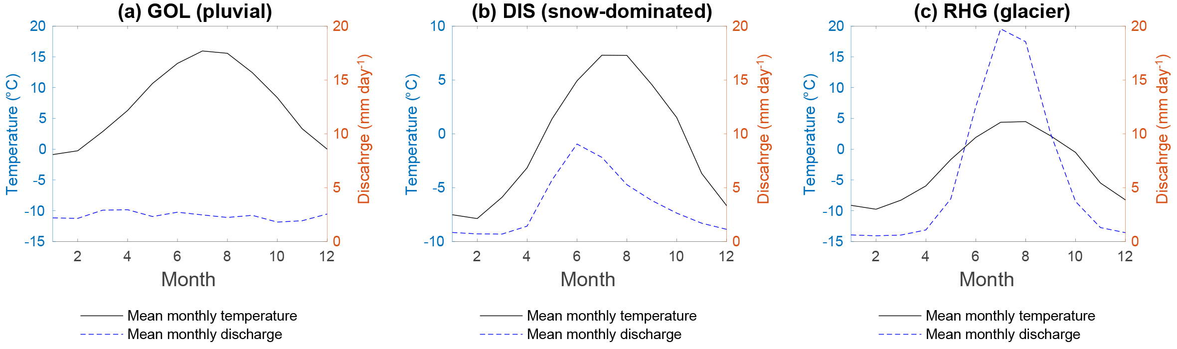
Figure 2Annual cycle of discharge and air temperature for three selected catchments representing three different hydrologic regimes (pluvial, snow-dominated and glacier). The mean monthly values computed over the entire observation period for each catchment are shown (see Table 1).
It is assumed here that discharge Q is the result of a series of rainfall inputs () that deliver enough water to fill the water deficit in the soil, i.e., that deliver enough water to raise the soil moisture level above its retention capacity. The excess water is removed from the soil as subsurface runoff and becomes river discharge. This description of the streamflow response neglects any direct surface flow.
The overall rainfall forcing ξ is modeled as a marked Poisson process with frequency λp and exponentially distributed rainfall depths with average α (average rainfall on rain days). Nevertheless, not all the rainfall events trigger streamflow responses, and the discharge-producing precipitation events ξ” are also modeled as a marked Poisson process with a decreased frequency λ<λp and the same α. λ is influenced by the soil storage capacity and soil drying time and can be written as (Botter et al., 2007a)
where Γ(a,b) is a lower incomplete Gamma function with parameters a and b, , and . E is the maximum evapotranspiration rate and nZr(s1−sw) synthesizes the soil volume liable to be filled by water before drainage starts; n is the porosity of the soil, Zr is the effective soil depth, s1 is the retention capacity and sw the permanent wilting point.

As discussed in detail by Botter et al. (2007c), this framework results in the following probability distribution of daily discharges at the catchment scale:
where A is the catchment area. This corresponds to a Gamma distribution with shape parameter λ∕k and a scale parameter αkA. The corresponding expected mean discharge equals . The model is suitable for steady-state conditions, at the annual or seasonal scale, depending on the temporal variability of the model parameters (Botter et al., 2007a).
Nonlinear storage–discharge relationships at the catchment scale are commonly observed (Botter et al., 2009; Brutsaert and Nieber, 1977; Mutzner et al., 2013). Accordingly, Botter et al. (2009) proposed an extension of the above modeling framework assuming that
where kn and a are the constants of the nonlinear recession. As for the linear model, it is possible to obtain an equation for the pdf of the daily discharges:
where C is a normalizing constant (Botter et al., 2009).
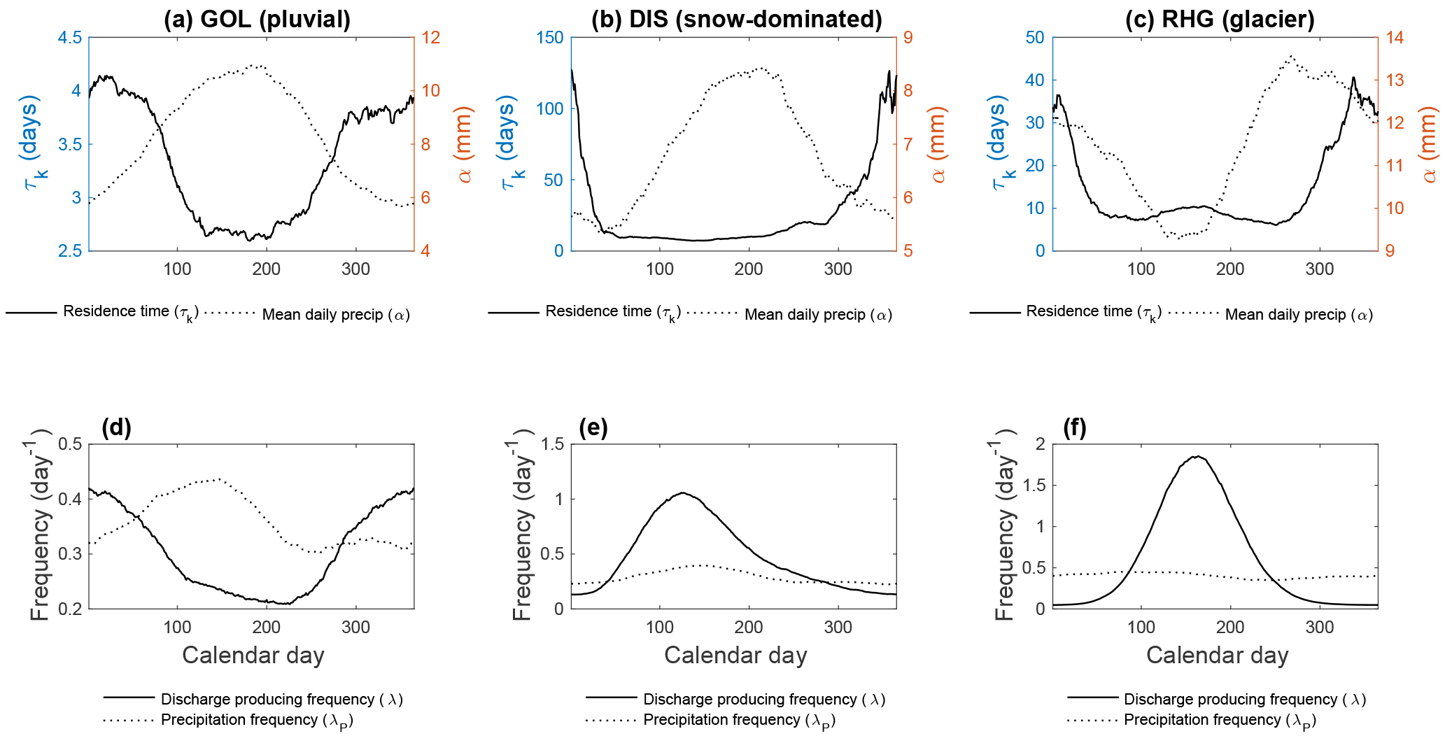
Figure 4Examples of the temporal variation of the model parameters over the course of a year. The parameters are calculated for 90-day intervals beginning at the calendar day for which the value is plotted; for a given time window, the data points corresponding to this window in all available civil years are pooled together. (a–c) Residence time τk and mean daily precipitation depth α. (d–f) Precipitation frequency λp and discharge-producing frequency λ.
2.2 Parameter estimation 1: forward estimation
We use the term “forward parameter estimation” to emphasize that the parameters are estimated directly from observed data, without calibration. This method is generally used in the context of this modeling framework for the estimation of the parameters related to the stochastic inputs (λp, α, λ), and this method is always used for these parameters in the present paper. However, the recession parameters (k, kn and a) are either estimated in a forward mode (Botter et al., 2007c, 2009; Ceola et al., 2010; Schaefli et al., 2013) or in an inverse mode (Ceola et al., 2010) (see Sect. 2.3).
The computation of the precipitation parameters first involves the computation of a reference catchment-scale precipitation time series (here obtained from gridded data; see Sect. 3). Then interception losses (I) are subtracted from the observed daily precipitation depths. These losses are in fact evaporated (or sublimated in case of snow) before participating to soil moisture dynamics. Following Rodriguez-Iturbe et al. (1999), previous model applications generally assumed that these losses are accounted for when the frequency of precipitation events is corrected to the frequency of discharge-producing events. In view of understanding how the model parameters vary in space, it was decided here to treat interception losses explicitly with minimal assumptions about this process: different maximum interception depths are attributed to four different land covers: 4 mm for forests, 2 mm for low vegetation, 1 mm for impervious areas and 0 mm for water bodies (Gerrits, 2010). The catchment-scale maximum interception depth is obtained as the land-use-weighted average of these values, but a minimum interception depth of 1 mm is imposed. This catchment-scale interception depth is subtracted from daily precipitation depths, assuming that at a daily time step, all intercepted water re-evaporates during the same time step.
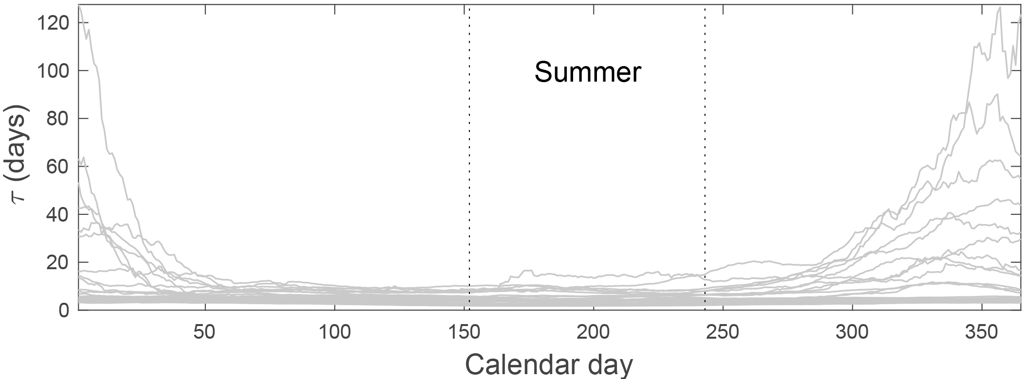
Figure 5Temporal variation of the residence time () for the 25 catchments. The temporal variation is obtained as in Fig. 4.
Instead of correcting the frequency of precipitation events λp according to Eq. (3), the frequency of discharge-producing events λ is estimated directly from the theoretical relationship between the mean discharge and the precipitation parameters, (see Eq. 4). Replacing the mean modeled discharge with the mean observed discharge , it follows that
Estimating λ from the above equation rather than directly from the soil properties as in Eq. (3) has been shown by Ceola et al. (2010) to provide much better results, and this method has been used by the majority of studies since then (e.g., Ceola et al., 2010; Botter et al., 2013; Basso et al., 2015).
The recession parameter for the linear model is calculated directly from observed daily discharge based on a classical Brutsaert–Nieber recession analysis (Brutsaert and Nieber, 1977; Biswal and Marani, 2010, 2014; Mutzner et al., 2013), considering, however, only discharges below a certain threshold, fixed to 95 %. The nonlinear recession parameters kn and a are also obtained from a recession analysis, using the same discharge threshold via linear regression of the logarithm of () versus the logarithm of Q, where a is the slope and kn the intercept.
2.3 Parameter estimation 2: inverse estimation
To objectively compare the potential of the linear and the nonlinear model formulations to capture observed flow-duration curves, the recession parameters for the linear model (k) and for the nonlinear model (kn,a) are also estimated in a classical inverse estimation mode where the model parameters are obtained by maximizing the likelihood function formulated for the model. For the linear model, the likelihood function is obtained from the model as follows:
where the probability p(.) is obtained from Eq. (4) and is the parameter vector containing all parameters that are estimated directly from observed data (i.e., not maximized). For the nonlinear case, the likelihood is obtained analogously by replacing k with kn and a and using p(.) from Eq. (6).
2.4 Model evaluation criteria
To objectively compare different models, we propose using the Kolmogorov–Smirnov distance between the cdfs corresponding to different models (Ceola et al., 2010; Schaefli et al., 2013), i.e., the maximum difference between the values of the empirical and the modeled cumulative distributions:
where corresponds to the empirical cumulative distribution of the discharges and F(Q) to the modeled cumulative distribution of the discharges. A good model should have a low cKS value.
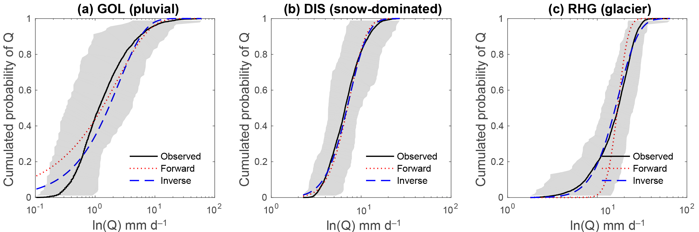
Figure 7Modeled cdfs with forward and inverse parameter estimation for the three selected catchments. The shaded area is located between the cdf envelopes and represents the natural variability of the daily discharges.
This comparison of the cdfs overcomes an important limitation inherent in the comparison of analytic pdfs and empirical pdfs. In fact, the choice of the number of classes for the calculation of the empirical pdf from observed data (via a so-called frequency polygon; Naghettini, 2016) can change the shape of the empirical pdf. The problem does not arise for cdfs given their cumulative nature.
Since the nonlinear model formulation has an additional parameter, the linear and the nonlinear models are also compared based on the Akaike information criterion (Burnham and Anderson, 2004; Laio et al., 2009; Ceola et al., 2010):
where n is the number of parameters of the model and ln is the logarithm of the maximum likelihood function obtained by maximizing Eq. (8). As for cKS, a good model should have a low cAIC value.
Based on the above criterion, we measure the relative performance increase from the linear to the nonlinear model as follows:
where is the Akaike criterion for the nonlinear model and for the linear model. Taking the opposite of the relative difference between the Akaike criteria ensures that a higher rAIC value indicates a stronger performance increase (recall that the Akaike criterion is to be minimized).
In addition, to assess the performance difference between different models, the obtained models are compared to the natural variability of the observed discharge cdfs. Therefore, an empirical long-term cdf is constructed, obtained by ranking the observed data in ascending order and dividing the rank numbers by the total sample size. Furthermore, to assess the natural yearly variability, individual cdfs are constructed for each summer season of each civil year (Vogel and Fennessey, 1994). From this collection of annual cdfs, envelopes are based on the maximum and minimum values of discharge for each probability class of the annual cdfs. A reliable model should yield a cdf contained between these curves and should be as close as possible to the long-term cdf.
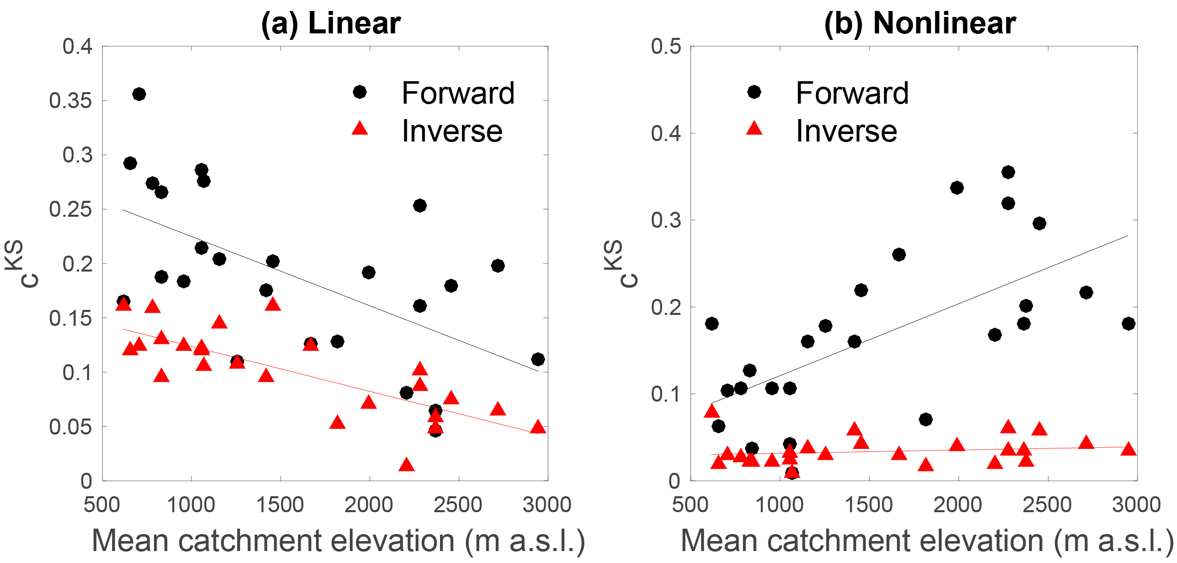
Figure 9Performance of the linear model and nonlinear model as a function of mean catchment elevation. The performance measure shown, cKS, is zero for a perfect model.
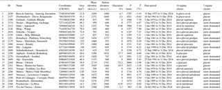
In this paper, we analyze 25 Swiss catchments with areas ranging from 1.05 to 377 km2 and with mean elevations ranging from 615 m a.s.l. (meters above sea level) to 2945 m a.s.l. (Table 1, Fig. 3). These catchments correspond to all streamflow gauging stations run by the Swiss Federal Office for the Environment (FOEN, 2017) and that have unperturbed discharges (i.e., minimal anthropogenic influence).
Table 1Characteristics of Swiss case study catchments as given in the FOEN database, including the FOEN identification code (ID), the catchment name, the Swiss coordinates of the gauging station, the drainage area, the mean elevation of the catchment and the gauging station elevation, the percentage of glacier-cover of the catchment, the mean annual precipitation, the mean annual temperature and the period of data acquisition. The 16 regime classes of Weingartner and Aschwanden (1992) are regrouped here into three classes (details are available in the Supplement).
The average precipitation at the country scale is around 1300 mm yr−1 (Blanc and Schädler, 2013). The complex topography leads to a high diversity of hydrologic regimes (Weingartner and Aschwanden, 1992), which can be grouped into (i) pluvial or rainfall-driven regimes, (ii) snow-dominated regimes and (iii) glacier regimes. Pluvial regimes are rainfall-dominated with sporadic snowfall events during winter; these regimes occur on the Swiss Plateau and in the Jura region (Fig. 3). Snow-dominated regimes result from seasonal snow cover, roughly at elevations above 900 m a.s.l. In these catchments, solid precipitation accumulates over several weeks up to several months during the cold season (winter) and is released entirely in the following spring and early summer. Glacier regimes result from perennial snow and ice accumulation at elevations roughly beyond 3000 m a.s.l. Most snow-dominated and glacier regimes are located in the Alps region (Fig. 3), few of them are located south of the Alps, which overall has a warmer climate and presents higher precipitation than the other two regions.
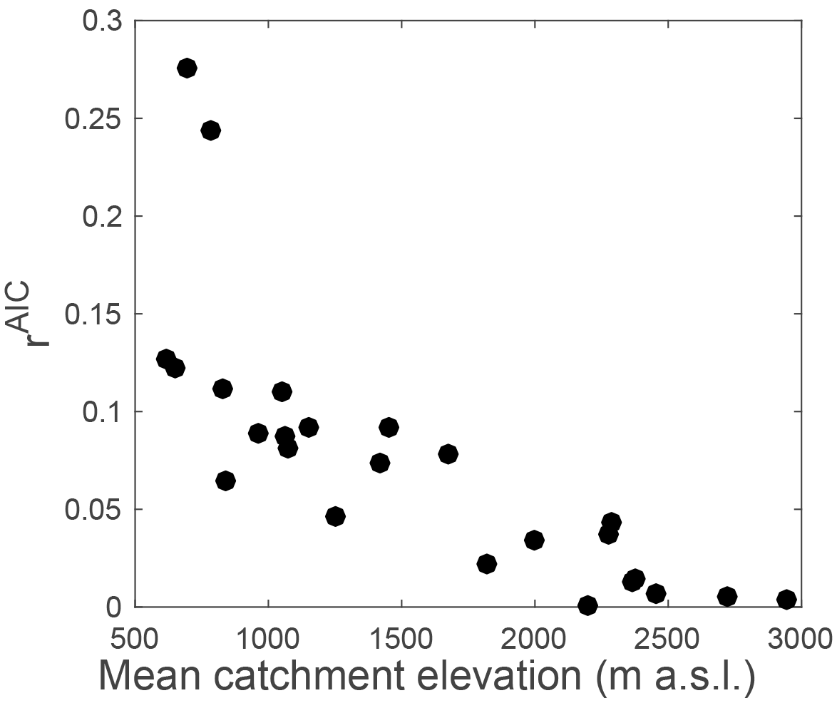
Figure 10Relative increase in the performance of the nonlinear model with respect to the linear model (as measured by rAIC) as a function of mean catchment elevation. All model parameters are estimated in inverse mode.
Most Swiss discharge regimes show a strong seasonality (Weingartner and Aschwanden, 1992), illustrated in Fig. 2 for typical examples of the three regime main types; air temperature is shown here as a proxy for snow and evapotranspiration processes. The pluvial Goldach River (GOL) shows the typical summer low flow resulting from evapotranspiration; the Dischmabach shows a snow regime with high summer flows resulting from the release of snowmelt stored in the subsurface during the main snowmelt period (spring) and from residual snowmelt during summer. The Rhône River (RHG) with its 50 % glacier cover shows a glacier regime, with significant ice melt during summer, and with monthly discharge peaking for the same month as air temperature (July).
It is noteworthy that surface runoff processes definitely can play a certain role in extreme events in all regions of Switzerland (Bernet et al., 2017), but all hydrologic regimes are dominated by subsurface runoff processes, a precondition for the application of the modeling framework developed by Botter et al. (2007c).
Besides observed daily discharge, the model requires catchment-scale daily precipitation as input. Most of the previous applications of the models used precipitation from one or several meteorological stations as input (Botter et al., 2007c, a, 2013; Ceola et al., 2010; Basso et al., 2015; Schaefli et al., 2013), which is potentially limiting for the model performance since good area-averaged input estimates are critical. Recent progress in spaceborne precipitation observation, and in particular the Global Precipitation Measurement (GPM) mission, potentially offers an interesting new data source for area-averaged precipitation estimates, even in such complex terrain as the Swiss Alps (Gabella et al., 2017), with the drawback of covering only short historical periods. Here, we use the relatively new spatial precipitation data set of MeteoSwiss with a nominal resolution of 2.2 km and an effective resolution between 15 and 20 km and extending back to 1961 (MeteoSwiss, 2011a). This data set can be assumed to give relatively good estimates of area-averaged precipitation (Paschalis et al., 2014; Addor and Fischer, 2015), even in mountainous areas where there are only few meteorological stations.
Corresponding catchment-scale average precipitation time series per case study catchment are obtained by averaging the daily precipitation time series of all pixels contained in the catchment (a list of pixels per catchment is included in the Supplement). In addition, we also used the corresponding gridded temperature data set (MeteoSwiss, 2011b) to support the analysis of parameter seasonality. As for precipitation, the catchment-scale average temperature data set is obtained by averaging the daily time series of all pixels.
Before estimating rainfall frequency (λp) and average rainfall depth on rain days (α), the catchment-scale precipitation time series are pre-processed to remove losses from interception. This step requires information about land use. Of the retained 25 case study catchments, 22 are part of what is called “hydrological study areas” and have an associated extended data set, including land use (Aschwanden, 1996). For the other catchments (i.e., the Areuse, Rhône-Gletsch and Venoge), land use is obtained from the Swiss land use database (Federal Statistical Office, 2001). Details about the land use estimation are available in the Supplement).
4.1 Discharge regimes and parameter seasonality
To gain further insights into the hydrological processes underlying the different regimes, Fig. 4 shows the within-year variability of the model parameters obtained by estimating the parameters in forward mode for moving and overlapping 90-day windows. The precipitation parameters α and λp do not show strong seasonal patterns, except for a few catchments such as the Goldach River (Fig. 4a). For snow and glacier regimes, the frequency of discharge-producing events, λ, increases strongly at the beginning of spring (Fig. 4b and c), which indicates the release of water from snowmelt or ice melt.
The inverse of the linear recession coefficient shows a coherent annual cycle for all catchments, independent of the underlying discharge regime (Fig. 5). This seasonal pattern with consistently low τ values during summer for all catchments clearly justifies the choice of a common summer season (June, July, August) for all regimes. The amplitude of the annual cycle (the difference between high and low τ values) is stronger for snow or glacier regimes, which reflects the fact that in these regimes, parts of the catchment are effectively dormant during the winter (Schaefli et al., 2013).
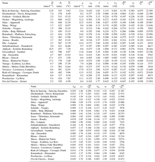
Table 2Parameter values and performance indicators for all the catchments for summer with linear model and forward estimation, summer linear model and inverse estimation, summer nonlinear model and forward estimation, winter nonlinear model and inverse estimation and winter linear model and forward estimation. stands for the mean observed discharge, Ps the mean total precipitation during summer, the mean temperature during summer, I for interception depth and cKS for the Kolmogorov–Smirnov distance. The indices stand for f, forward estimation; i, inverse estimation; l, linear model; n, nonlinear model.
4.2 Linear model
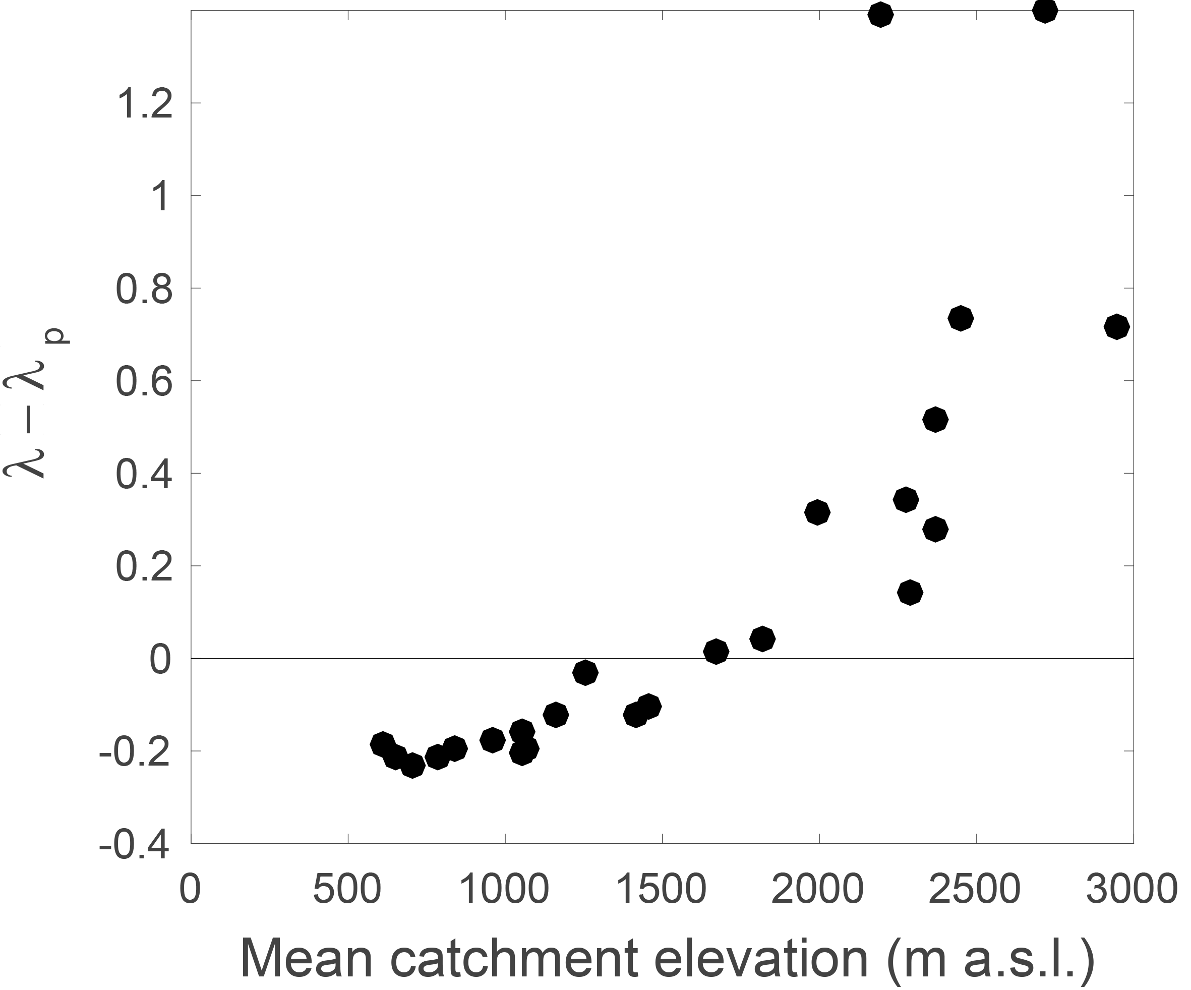
All estimated parameters for both forward and inverse estimations are summarized in Table 2, together with the values of the performance indicator cKS. It can be noted that for 11 catchments (i.e., Rein da Sumvitg, Dischmabach, Alpbach, Grosstalbach, Rhône à Gletsch, Massa, Verzasca, Riale di Calneggia, Krummbach, Poschiavino and Ova da Cluozza), λ exceeds λp, contradicting the original description of the model (Botter et al., 2007b), which states that the discharge-producing frequency λ is smaller than the precipitation frequency λp. Such an exceedance of λ over λp should only happen in catchments or seasons with an additional source of water (in addition to rainfall), which in the present case is snowmelt or ice melt.
The exceedance of λ over λp increases with mean catchment elevation (Fig. 6), the limit of λ=λp being at around 1500 m a.s.l. This important result is further discussed in Sect. 5.
The cdfs obtained from all estimated parameters are presented in Fig. 7 for the three example case studies. For the catchment with rainfall-driven discharges (GOL), it can be seen that the probabilities of occurrence of low flows are largely overestimated with forward estimation (Fig. 7a). This is a typical indication that the recession timescale is underestimated. The model values even exceed the envelopes that represent the natural variability of the discharges. In the presence of snow, the linear model in forward estimation mode tends to underestimate low flows, with satisfactory results for some cases, such as the Dischmabach (Fig. 7b).
Overall, there is a strong increasing trend of the linear model performance with mean catchment elevation (Fig. 9a). Despite this, the results of the linear model are not satisfactory for the forward estimation method for any of the regimes.
The inverse estimation of the model parameters improves the results significantly, but the cKS performance indicator shows relatively high values and the curves are visually not accurate, especially for pluvial regimes. This suggests that the model with a linear discharge decay is overall not suitable for the studied catchments.
4.3 Nonlinear models
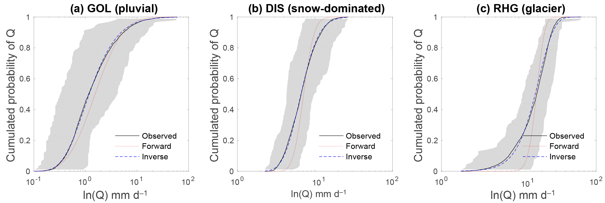
The results obtained from inverse parameter estimation for the nonlinear model are very good (Fig. 8, Table 2), and the nonlinear model outperforms the linear model for all catchments, both in terms of the KS performance and in terms of the Akaike criterion (Table 2). The relative model performance increase (as measured by rAIC) shows furthermore a strong inverse trend with mean catchment elevation (Fig. 10), which results from the increasing performance of the linear model with increasing elevation (Fig. 9b).
It is noteworthy that the two catchments for which the performance increase in the nonlinear model over the linear models exceeds 20 % are the two catchments that have a strongly karst-influenced regime (Scheulte at Vicques and Venoge at Ecublens).
As for the linear model, the forward estimation mode gives worse results than the inverse estimation mode. For some catchments (i.e., Murg-Wängi, Gürbe, Sense, Ilfis, and Grosstalbach), the forward estimation mode gives nevertheless very good results with cKS below 0.1. In general, for the catchments where the discrepancies between modeled and observed cdfs are due to an underestimation of τ, the nonlinear model yields a significant improvement. For catchments where the recession timescale is overestimated with the linear model, the nonlinear model in forward mode leads to a performance decrease.
Our results show that analytical modeling framework for streamflow distributions proposed by Botter et al. (2007c) performs well for the 25 Swiss catchments across all studied discharge regimes. A detailed comparison between the performance of the linear and the nonlinear models considering the optimized parameters obtained from the inverse approach shows that the results for the nonlinear model are always better than for the linear model. This underlines that the nonlinear recession is better suited for the hydrological conditions of all studied catchments, which is in line with previous results (Ceola et al., 2010; Basso et al., 2015).
In forward estimation mode, the linear model outperforms the nonlinear model for catchments with summer high flows; the nonlinear model outperforms the linear model for catchments with rainfall-driven regimes (i.e., summer low flows). This results from the fact that for regimes with summer high flow, the linear model overestimates the recession timescale (resulting in a underestimation of the discharge variance). For regimes with summer low flow, the linear model in exchange underestimates the recession timescale. Given that the nonlinear model yields longer recessions, the nonlinear model shows accordingly a better performance for regimes with summer low flow.
The comparison between the forward and inverse estimation methods shows a clear underestimation of kn for most of the catchments, which was already discussed by Dralle et al. (2015) and which is in line with previous work that tried to improve the results of the model in forward estimation mode, for the linear and the nonlinear formulation (Ceola et al., 2010; Basso et al., 2015). There is clearly a need to further improve the methods to estimate the recession parameters. Our results pinpoint that a key here might be the detailed investigation of recession analysis methods along elevational gradients and related hydrologic regimes.
Overall, good model performance in many different catchments with different regimes indicates that the modeling framework is suitable for the prediction of FDCs in Switzerland. A more detailed temporal model validation (e.g., with a split sample test; Klemeš, 1986) is not possible for this framework since the model parameters are obtained directly from observed data for each time period (i.e., they vary from period to period). The obtained model performances are comparable to the results obtained in previous studies, e.g., in the work of Ceola et al. (2010). For different case studies in Italy and the US, they obtained cKS values varying between 0.030 and 0.409 for the nonlinear model using different methods of forward estimation, and cKS values between 0.021 to 0.051 for inverse estimation. For the linear model, Ceola et al. (2010) obtained cKS values between 0.054 and 0.567. Basso et al. (2015) and Doulatyari et al. (2017) studied some case studies that are included in the present paper (Sitter at Appenzell and Murg at Wängi).
Recomputing their results with their model parameters yields slightly different cKS values for the nonlinear model for the Sitter (0.12 compared to our 0.19) and for the Murg (0.05 to 0.06 compared to our 0.06). These differences are small and can be explained by different data periods and by the methodological choices in the calculation of parameters.
The most remarkable result of the presented analysis is the fact that the modeling framework is applicable in its original formulation to catchments where summer flow is influenced by snow processes. The additional source of water from snow or ice melt is accommodated by increasing the frequency λ of discharge-producing events. This is in line with a common assumption in catchment-scale precipitation–runoff modeling (e.g., Schaefli et al., 2005), which is that runoff from snowmelt can be modeled with exactly the same functional relationships as for rainfall, by simply feeding so-called equivalent precipitation (sum of rainfall and simulated snowmelt) into the runoff-generation module.
Furthermore, the increase in the discharge-producing frequency to account for snow or ice melt is also coherent with the original description of the analytic modeling framework, which incorporates losses as a decrease in the discharge-producing frequency. This type of behavior can be identified in previous studies. For the Sitter at Appenzell, Basso et al. (2015) obtained λ values that are close to the precipitation frequency λp during spring; for the Thur at Jonschwil they obtained λ=λp for spring. Both catchments have a mean elevation above 1000 m a.s.l., which suggests the presence of snow processes. Later on, Doulatyari et al. (2017) discussed that snow accumulation and melt could be affecting the streamflow pdf estimation for the Sitter at Appenzell, without, however, exploring the issue further.
As can be seen in Fig. 6, the switch from λ<λp to λp to λ>λp is located at around 1500 m a.s.l. This corresponds to a relatively low mean catchment elevation; for this mean elevation, it can a priori not be assumed that significant snowmelt continues throughout the summer. In fact, for most snow-influenced catchments, the majority of snowmelt happens during spring. Summer flows are nevertheless directly influenced by spring snowmelt since the summer discharge results from a continuous release of melt water stored in the catchment during the preceding snowmelt period. For high elevation catchments, the exceedance of λ over λp is directly related to significant snowmelt and ice melt inputs throughout the summer.
It should be kept in mind here that for the present study, λ is estimated directly from the relationship between discharge and precipitation (see Sect. 2.2 and Eq. 7). The question of how to estimate this parameter directly from catchment characteristics based on long-term snow cover statistics and data on glacier cover remains to be answered in future work.
Besides the important result that the model is applicable to snow-influenced catchments, additional insights can be obtained from the highlighted model performance trends with mean catchment elevation (Figs. 9 and 10). These performance trends are explained by the evolution of the regimes with mean catchment elevation, from rainfall-dominated (pluvial) regimes with summer low flow to snowfall-influenced (nival and glacier) regimes with summer high flow. This result suggests that mean catchment elevation is a good proxy for regime shifts, despite the fact that many other catchment characteristics vary strongly across the set of studied catchments (area, hypsometric curve, land use, etc.). Given the strong link between mean catchment elevation, mean catchment air temperature and snow accumulation, this opens interesting perspectives for parameter regionalization.
This application of the analytic framework of Botter et al. (2007c) to estimate summer streamflow probability distributions for 25 Swiss catchments shows that this framework performs well without any further methodological adjustments across a wide range of discharge regimes, including rainfall-driven regimes with summer low flows, but also regimes with snowmelt- and glacier-melt-influenced summer high flows. Given that the original framework was developed for purely rainfall-driven regimes, this result is unexpected. For snow-influenced catchments, the model has been shown here to accommodate the additional source of water from snowmelt by a relative increase in the discharge-producing frequency, which is coherent with the underlying analytic framework.
The detailed comparison between the performance of the linear and the nonlinear model formulation shows that the description of Swiss summer flows strongly benefits from using a nonlinear storage–discharge relationship, in particular for catchments with summer low flow and for the karst catchments. In general, the linear model performance increases for increasing total summer flows or, equivalently, for catchments with higher mean elevation. Future work will focus on improving the model parameter estimation directly from observed data (without parameter optimization), which is a precondition for parameter regionalization. Better insights into the physical drivers of the different parameters will also open new potential for extending the model framework to all four seasons for all Swiss streamflow regimes.
The meteorological data used are not currently freely available; they require a license from MeteoSwiss. The discharge data are available upon request from the Swiss Federal Office for the Environment at https://www.hydrodaten.admin.ch/en/ (last access: 15 December 2017, FOEN, 2017). The basin boundaries used, obtained from the Swiss Federal Office for the Environment, are available in the Supplement as vector files.
The supplement related to this article is available online at: https://doi.org/10.5194/hess-22-2377-2018-supplement.
The authors declare that they have no conflict of interest.
The work of the first author is funded by the Portuguese Science and
Technology Foundation (FCT), grant no. PD/BD/52663/2014. The work of
Bettina Schaefli is funded by the Swiss National Science Foundation (SNSF), grant
no. PP00P2_157611. We thank the editor, Fabrizio Fenicia, and two anonymous
reviewers for their detailed comments on an earlier version of this
manuscript.
Edited by: Fabrizio Fenicia
Reviewed by: two anonymous referees
Addor, N. and Fischer, E. M.: The influence of natural variability and interpolation errors on bias characterization in RCM simulations, J. Geophys. Res.-Atmos., 120, 10180–10195, https://doi.org/10.1002/2014JD022824, 2015. a
Aschwanden, A.: Caractéristiques physiographiques des bassins de recherches hydrologiques en Suisse, Berne, Service hydrologique et géologique national, Communications hydrologiques, 23, 1996. a
Basso, S., Schirmer, M., and Botter, G.: On the emergence of heavy-tailed streamflow distributions, Adv. Water Res., 82, 98–105, https://doi.org/10.1016/j.advwatres.2015.04.013, 2015. a, b, c, d, e, f, g, h, i
Bernet, D. B., Prasuhn, V., and Weingartner, R.: Surface water floods in Switzerland: what insurance claim records tell us about the damage in space and time, Nat. Hazards Earth Syst. Sci., 17, 1659–1682, https://doi.org/10.5194/nhess-17-1659-2017, 2017. a
Biswal, B. and Marani, M.: Geomorphological origin of recession curves, Geophys. Res. Lett., 37, 24, https://doi.org/10.1029/2010gl045415, 2010. a
Biswal, B. and Marani, M.: “Universal” recession curves and their geomorphological interpretation, Adv. Water Res., 65, 34–42, https://doi.org/10.1016/j.advwatres.2014.01.004, 2014. a
Blanc, P. and Schädler, B.: Water in Switzerland – an overview, Tech. rep., available at: http://www.naturalsciences.ch/topics/water/ (in English; last access: 18 August 2015), 2013. a
Botter, G., Peratoner, F., Porporato, A., Rodriguez-Iturbe, I., and Rinaldo, A.: Signatures of large-scale soil moisture dynamics on streamflow statistics across U.S. climate regimes, Water Resour. Res., 43, https://doi.org/10.1029/2007wr006162, 2007a. a, b, c, d, e
Botter, G., Porporato, A., Daly, E., Rodriguez-Iturbe, I., and Rinaldo, A.: Probabilistic characterization of base flows in river basins: Roles of soil, vegetation, and geomorphology, Water Resour. Res., 43, https://doi.org/10.1029/2006wr005397, 2007b. a
Botter, G., Porporato, A., Rodriguez-Iturbe, I., and Rinaldo, A.: Basin-scale soil moisture dynamics and the probabilistic characterization of carrier hydrologic flows: Slow, leaching-prone components of the hydrologic response, Water Resour. Res., 43, w02417, https://doi.org/10.1029/2006WR005043, 2007c. a, b, c, d, e, f, g, h, i, j
Botter, G., Porporato, A., Rodriguez-Iturbe, I., and Rinaldo, A.: Nonlinear storage-discharge relations and catchment streamflow regimes, Water Resour. Res., 45, https://doi.org/10.1029/2008wr007658, 2009. a, b, c, d, e, f
Botter, G., Basso, S., Rodriguez-Iturbe, I., and Rinaldo, A.: Resilience of river flow regimes, P. Natl. Acad. Sci. USA, 110, 12925–12930, https://doi.org/10.1073/pnas.1311920110, 2013. a, b, c, d, e
Brutsaert, W. and Nieber, J. L.: Regionalized drought flow hydrographs from a mature glaciated plateau, Water Resour. Res., 13, 637–643, https://doi.org/10.1029/wr013i003p00637, 1977. a, b
Burnham, K. P. and Anderson, D. R. (Eds.): Model Selection and Multimodel Inference, Springer New York, https://doi.org/10.1007/b97636, 2004. a
Castellarin, A., Botter, G., Hughes, D. A., Liu, S., Ouarda, T. B. M. J., Parajka, J., Post, D. A., Sivapalan, M., Spence, C., Viglione, A., and Vogel, R. M.: Prediction of flow duration curves in ungauged basins, Runoff prediction in ungauged basins: Synthesis across processes, places and scales, Cambridge University Press, 135–162, 2013. a
Ceola, S., Botter, G., Bertuzzo, E., Porporato, A., Rodriguez-Iturbe, I., and Rinaldo, A.: Comparative study of ecohydrological streamflow probability distributions, Water Resour. Res., 46, https://doi.org/10.1029/2010wr009102, 2010. a, b, c, d, e, f, g, h, i, j, k, l, m, n, o, p
Doulatyari, B., Betterle, A., Basso, S., Biswal, B., Schirmer, M., and Botter, G.: Predicting streamflow distributions and flow duration curves from landscape and climate, Adv. Water Res., 83, 285–298, https://doi.org/10.1016/j.advwatres.2015.06.013, 2015. a
Doulatyari, B., Betterle, A., Radny, D., Celegon, E. A., Fanton, P., Schirmer, M., and Botter, G.: Patterns of streamflow regimes along the river network: The case of the Thur river, Environ. Modell. Softw., 93, 42–58, https://doi.org/10.1016/j.envsoft.2017.03.002, 2017. a, b, c, d
Dralle, D., Karst, N., and Thompson, S. E.: a, b careful: The challenge of scale invariance for comparative analyses in power law models of the streamflow recession, Geophys. Res. Lett., 42, 9285–9293, 2015. a
Swiss Federal Office for Statistics: Geostat – Version 1997, Swiss spatial land use statistics data-base (Arealstatistik der Schweiz 1979/85 und Arealstatistik der Schweiz 1992/97), Neuchâtel, Switzerland, 35 p, 2001. a
Federal Office for the Environment: Biogeographical regions of Switzerland (CH), available at: https://opendata.swiss/en/dataset/biogeographische-regionen-der-schweiz-ch (last access: 15 December 2017), 2004. a
FOEN: Hydrological data and forecasts, Federal Office for the Environment (FOEN), Bern, Switzerland, available at: https://www.hydrodaten.admin.ch/en/stations-and-data.html, last access: 15 December 2017. a, b
Gabella, M., Speirs, P., Hamann, U., Germann, U., and Berne, A.: Measurement of Precipitation in the Alps Using Dual-Polarization C-Band Ground-Based Radars, the GPM Spaceborne Ku-Band Radar, and Rain Gauges, Remote Sens., 9, 1147, https://doi.org/10.3390/rs9111147, 2017. a
Gerrits, A. M. J.: The role of interception in the hydrological cycle, TU Delft, Delft University of Technology, 2010. a
Helbling, A.: Topographical catchments of the FOEN gauging stations. Geodataset EZG hydrometrische Stationen, Tech. rep., available at http://www.bafu.admin.ch/wasser/13462/13496/15010/ index.html?lang=en, last access: 11 May 2017, 2016. a
Klemeš, V.: Operational testing of hydrological simulation models, Hydrol. Sci. J., 31, 13–24, https://doi.org/10.1080/02626668609491024, 1986. a
Laio, F., Baldassarre, G. D., and Montanari, A.: Model selection techniques for the frequency analysis of hydrological extremes, Water Resour. Res., 45, https://doi.org/10.1029/2007wr006666, 2009. a
MeteoSwiss, F. O. o. M. a. C.: Documentation of MeteoSwiss Grid-Data Products: Daily mean, minimum and maximum temperature, MeteoSwiss, Zürich, 4, 2011a. a
MeteoSwiss, F. O. o. M. a. C.: Documentation of MeteoSwiss Grid-Data Products: Daily Precipitation (final analysis): RhiresD, MeteoSwiss, Zürich, 4, 2011b. a
Müller, M. F. and Thompson, S. E.: Comparing statistical and process-based flow duration curve models in ungauged basins and changing rain regimes, Hydrol. Earth Syst. Sci., 20, 669–683, https://doi.org/10.5194/hess-20-669-2016, 2016. a
Müller, M. F., Dralle, D. N., and Thompson, S. E.: Analytical model for flow duration curves in seasonally dry climates, Water Resour. Res., 50, 5510–5531, https://doi.org/10.1002/2014wr015301, 2014. a
Mutzner, R., Bertuzzo, E., Tarolli, P., Weijs, S. V., Nicotina, L., Ceola, S., Tomasic, N., Rodriguez-Iturbe, I., Parlange, M. B., and Rinaldo, A.: Geomorphic signatures on Brutsaert base flow recession analysis, Water Resour. Res., 49, 5462–5472, https://doi.org/10.1002/wrcr.20417, 2013. a, b
Naghettini, M.: Preliminary Analysis of Hydrologic Data, in: Fundamentals of Statistical Hydrology, 21–56, Springer International Publishing, https://doi.org/10.1007/978-3-319-43561-9_2, 2016. a
Paschalis, A., Fatichi, S., Molnar, P., Rimkus, S., and Burlando, P.: On the effects of small scale space-time variability of rainfall on basin flood response, J. Hydrol., 514, 313–327, https://doi.org/10.1016/j.jhydrol.2014.04.014, 2014. a
Rodriguez-Iturbe, I., Porporato, A., Ridolfi, L., Isham, V., and Coxi, D. R.: Probabilistic modelling of water balance at a point: the role of climate, soil and vegetation, P. Roy. Soc. A-Math. Phy., 455, 3789–3805, https://doi.org/10.1098/rspa.1999.0477, 1999. a, b, c
Schaefli, B., Hingray, B., Niggli, M., and Musy, A.: A conceptual glacio-hydrological model for high mountainous catchments, Hydrol. Earth Syst. Sci., 9, 95–109, https://doi.org/10.5194/hess-9-95-2005, 2005. a
Schaefli, B., Rinaldo, A., and Botter, G.: Analytic probability distributions for snow-dominated streamflow, Water Resour. Res., 49, 2701–2713, https://doi.org/10.1002/wrcr.20234, 2013. a, b, c, d, e, f, g
Searcy, J. K.: Flow-duration curves, US Government Printing Office, 1959. a
SwissTopo: DHM25- The digital height model of Switzerland DHM25, Product information, Wabern, Bern, 15, 2005. a
Vogel, R. M. and Fennessey, N. M.: Flow-Duration Curves I: New Interpretation and Confidence Intervals, J. Water Res. Plann. Manage., 120, 485–504, https://doi.org/10.1061/(asce)0733-9496(1994)120:4(485), 1994. a, b, c
Vogel, R. M. and Fennessey, N. M.: Flow duration curves II: a review of the applications in water resources planning, J. Am. Water Res. Assoc., 31, 1029–1039, https://doi.org/10.1111/j.1752-1688.1995.tb03419.x, 1995. a
Weingartner, R. and Aschwanden, H.: Discharge regime–the basis for the estimation of average flows, Hydrological Atlas of Switzerland, Plate, 5, 26, 1992. a, b, c