the Creative Commons Attribution 3.0 License.
the Creative Commons Attribution 3.0 License.
Analyzing the future climate change of Upper Blue Nile River basin using statistical downscaling techniques
Dagnenet Fenta Mekonnen
Markus Disse
Climate change is becoming one of the most threatening issues for the world today in terms of its global context and its response to environmental and socioeconomic drivers. However, large uncertainties between different general circulation models (GCMs) and coarse spatial resolutions make it difficult to use the outputs of GCMs directly, especially for sustainable water management at regional scale, which introduces the need for downscaling techniques using a multimodel approach. This study aims (i) to evaluate the comparative performance of two widely used statistical downscaling techniques, namely the Long Ashton Research Station Weather Generator (LARS-WG) and the Statistical Downscaling Model (SDSM), and (ii) to downscale future climate scenarios of precipitation, maximum temperature (Tmax) and minimum temperature (Tmin) of the Upper Blue Nile River basin at finer spatial and temporal scales to suit further hydrological impact studies. The calibration and validation result illustrates that both downscaling techniques (LARS-WG and SDSM) have shown comparable and good ability to simulate the current local climate variables. Further quantitative and qualitative comparative performance evaluation was done by equally weighted and varying weights of statistical indexes for precipitation only. The evaluation result showed that SDSM using the canESM2 CMIP5 GCM was able to reproduce more accurate long-term mean monthly precipitation but LARS-WG performed best in capturing the extreme events and distribution of daily precipitation in the whole data range.
Six selected multimodel CMIP3 GCMs, namely HadCM3, GFDL-CM2.1, ECHAM5-OM, CCSM3, MRI-CGCM2.3.2 and CSIRO-MK3 GCMs, were used for downscaling climate scenarios by the LARS-WG model. The result from the ensemble mean of the six GCM showed an increasing trend for precipitation, Tmax and Tmin. The relative change in precipitation ranged from 1.0 to 14.4 % while the change for mean annual Tmax may increase from 0.4 to 4.3 ∘C and the change for mean annual Tmin may increase from 0.3 to 4.1 ∘C. The individual result of the HadCM3 GCM has a good agreement with the ensemble mean result. HadCM3 from CMIP3 using A2a and B2a scenarios and canESM2 from CMIP5 GCMs under RCP2.6, RCP4.5 and RCP8.5 scenarios were downscaled by SDSM. The result from the two GCMs under five different scenarios agrees with the increasing direction of three climate variables (precipitation, Tmax and Tmin). The relative change of the downscaled mean annual precipitation ranges from 2.1 to 43.8 % while the change for mean annual Tmax and Tmin may increase in the range from 0.4 to 2.9 ∘C and from 0.3 to 1.6 ∘C respectively.


The impacts of climate change on the hydrological cycle in general and on water resources in particular are of high significance due to the fact that all natural and socioeconomic systems critically depend on water. The direct impact of climate change can be variation and changing pattern of water resources availability and hydrological extreme events such as floods and droughts, with many indirect effects on agriculture, food and energy production and overall water infrastructure (Ebrahim et al., 2013). The impact may be worse on transboundary rivers like the Upper Blue Nile River where competition for water is becoming high from different economic, political and social interests of the riparian countries and when runoff variability of upstream countries can greatly affect the downstream countries (Kim, 2008; Semenov and Barrow, 1997).
According to IPCC (2007), between 75 and 250 million people are projected to be exposed to increased water stress due to climate change in Africa by 2020. The increasing water demand of upstream countries in the Nile Basin coupled with climate change impacts can affect the availability of water resources for downstream countries and in the basin, which could result in resource conflicts and regional insecurities. Moreover, climate variability (i.e., the way climate fluctuates yearly and seasonally above or below a long-term average value, caused by changes in forcing factors such as variation in seasonal extent of the intertropical convergence zone like El Niño and La Niña events) is already imposing a significant challenge to Ethiopia by affecting food security, water and energy supply, poverty reduction, and sustainable socioeconomic development efforts. To mitigate these challenges, the Ethiopian government therefore carried out a series of studies on Upper Blue Nile River basin (UBNRB), which has been identified as an economic “growth corridor”, focused on identifying irrigation and hydropower potential of the basin (BCEOM, 1998; USBR, 1964; WAPCOS, 1990). As a result, large-scale irrigation and hydropower projects including the Grand Ethiopian Renaissance Dam (GERD), the largest hydroelectric power plant in Africa, have been identified and are being constructed as mitigation measures for the impacts of climate change. However, most studies have put less emphasis on climate change and its impact on the hydrology of the basin, and hence identifying local impacts of climate change at basin level is quite important. This is especially important in the UBNRB for the sustainability of large-scale water resource development projects, for proper water resource management leading to regional security and for finding possible mitigation measures to avoid catastrophic consequences.
To this end, several individual studies have been done to study the impacts of climate change on the water resources of Upper Blue Nile River basin. Taye et al. (2011) reviewed some of the research outputs and concluded that clear discrepancies were observed, particularly on the projection of precipitation. For instance, as the results obtained from Bewket and Conway (2007), Conway (2000) and Gebremicael et al. (2013) showed, there is no significant trend observed in the amount of seasonal and annual rainfall, while Mengistu et al. (2014) reported statistically nonsignificant increasing trends in annual and seasonal rainfall. For the future projection, expected changes in precipitation amount are unclear. For instance, Kim (2008) used the outputs of six GCMs for the projection of future precipitations and temperature, and the result suggested that the changes in mean annual precipitation from the six GCMs range from −11 to 44 % with a change of 11 % from the weighted average scenario in the 2050s. However, the changes in mean annual temperature range from 1.4 to 2.6 ∘C with a change of 2.3 ∘C from the weighted average scenario. Likewise, Yates and Strzepek (1998a) used three GCMs and the result revealed that the changes in precipitation range from −5 to 30 % and the changes in temperature range from 2.2 to 3.5 ∘C. Yates and Strzepek (1998b) also used six GCMs and the result showed in the range from −9 to 55 % for precipitation while temperature increased from 2.2 to 3.7 ∘C. Another study done by Elshamy et al. (2009), used 17 GCMs and the result showed that changes in total annual precipitation range between −15 to 14 % but the ensemble mean of all models showed almost no change in the annual total rainfall, while all models predict the temperature to increase between 2 and 5 ∘C. Gebre and Ludwig (2015) used five bias-corrected 50 km × 50 km spatial resolution GCMs for RCP4.5 and RCP8.5 scenarios to downscale the future climate change of four watersheds (Gilgel Abay, Gumara, Ribb and Megech) located in Tana subbasin for the time period of 2030s and 2050s (the time periods of 2011–2040, 2041–2070 and 2071–2100 are referred to throughout as the 2030s, 2050s and 2080s, respectively). The result suggested that the selected five GCMs disagree on the direction of future prediction of precipitation, but multimodal average monthly and seasonal precipitation may generally increase over the watersheds.
For the historical context, the discrepancies could be due to the period and length of data analyzed and the failure to consider stations which can represent the spatial variability of the basin and also errors induced from observed data. For the future context, besides the abovementioned reasons, discrepancies could be due to the differences in GCMs and scenarios used for downscaling, the downscaling techniques applied (can be dynamical and statistical), selection of representative predictors, the period of analysis, and spatial and temporal resolution of observed and predictor data sets.
To address uncertainty in projected climate changes, the IPCC (2014) thus recommends using a large ensemble of climate change scenarios produced from various combinations of atmospheric ocean general circulation models (AOGCMs) and forcing scenarios. However, it can become prohibitively time consuming to assess the climate change using many climate change scenarios and many statistical downscaling models simultaneously. As a result, researchers typically assess climate change and its impacts under only one or a few climate change scenarios, selected arbitrarily with no justification, for instance those that used only A1B and A2 scenarios. Yet there is no any hard rule to select an appropriate subset of climate change scenarios among the wide range of possibilities (Casajus et al., 2016).
GCMs perform reasonably well at larger spatial scales but poorly at finer spatial and temporal scales, especially precipitation, which is of interest in hydrological impact analysis (Goly et al., 2014). Hence, the processes of downscaling that ensure that the scale discrepancy between the coarse-scale GCMs and the required local-scale climate variables for hydrological models will be narrowed down should be investigated for their contribution, which has often been overlooked in previous studies on climate change analysis in the UBNRB. Many researchers have tried to compare the comparative skill of downscaling methods in different study areas (Dibike and Coulibaly, 2005; Ebrahim et al., 2013; Fiseha et al., 2012; Goodarzi et al., 2015; Hashmi et al., 2011; Khan et al., 2006; Qian et al., 2004; Wilby et al., 2004; Wilby and Wigley, 1997; Xu, 1999). However, no single model has been found to perform well over all the regions and timescales. Thus, evaluations of different models is critical to understanding the applicability of the existing models.
Apart from the GCMs and downscaling techniques, most of the previous studies (e.g., Beyene et al. (2010), Elshamy et al. (2009) and Kim (2008)) used CRU, NFS and other gridded data sets constructed based on the interpolation of a few stations in Ethiopia, which are relatively less accurate compared with the station-based data (Worqlul et al., 2014). Therefore, the objective of this study is (i) to evaluate the comparative performance of two widely used statistical downscaling techniques, namely the Long Ashton Research Station Weather Generator (LARS-WG) and the Statistical Downscaling Model (SDSM) over the UBNRB, and (ii) to downscale future climate scenarios of precipitation, maximum temperature (Tmax) and minimum temperature (Tmin) at acceptable spatial and temporal resolution, which can be used directly for further hydrological impact studies. This can be achieved through applying a multimodel approach, to minimize the uncertainty of GCMs and incorporate acceptable number of weather stations which have long time series and reliable observed climate data to minimize the errors coming from the less accurate gridded data sets.
Generally, downscaling methods are classified into dynamic and statistical downscaling (Fowler et al., 2007; Wilby et al., 2002). Dynamic downscaling nests higher-resolution regional climate models (RCMs) into coarse-resolution GCMs to produce complete set of meteorological variables which are consistent with each other. The outputs from this method are still not at the scale that the hydrological model requires. Statistical downscaling overcomes this challenge; moreover it is computationally undemanding, simple to apply and provides the possibility of uncertainty analysis (Dibike et al., 2005; Semenov et al., 1997; Wilby et al., 2002). Extensive details on the strength and weakness of the two methods can be found in Wilby et al. (2007, 1997). Among the different possibilities, two well-recognized statistical downscaling tools, a regression-based SDSM (Wilby et al., 2002) and a stochastic weather generator, LARS-WG (Semenov et al., 1997, 2002) were chosen for this study. They have been tested in various regions (e.g., Chen et al., 2013; Dibike et al., 2005; Dile et al., 2013; Elshamy et al., 2009; Fiseha et al., 2012; Hashmi et al., 2011; Hassan et al., 2014; Maurer and Hidalgo, 2008; Yimer et al., 2009) under different climatic conditions of the world.
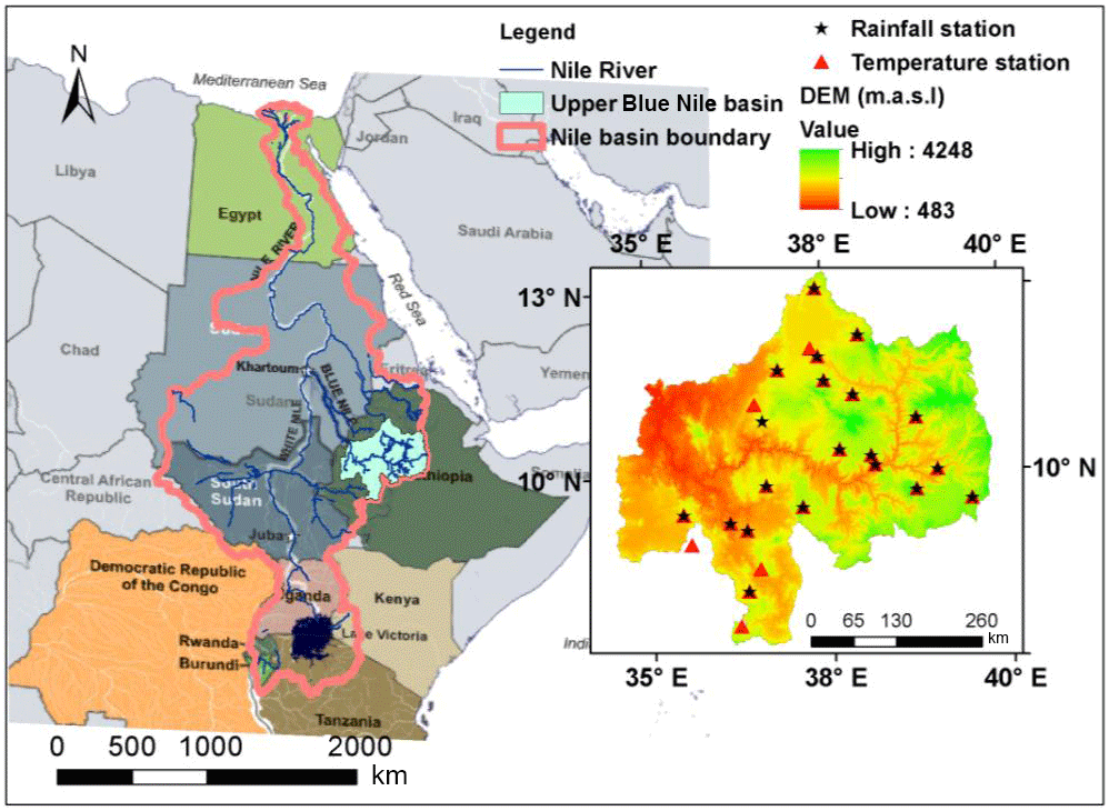
The Upper Blue Nile River basin extends from 7∘45′ to 13∘ N and 34∘30′ and 37∘45′ E; see Fig. 1. It is one of the most important major basins of Ethiopia because it contributes to 45 % of the countries surface water resources, 20 % of the population, 17 % of the landmass, 40 % of the nation's agricultural product and a large portion of the hydropower and irrigation potential of the country (Elshamy et al., 2009). The whole UBNRB has an area coverage of 199 812 km2 (BCEOM, 1998). For this study, Rahad, Gelegu and Dinder subcatchments that do not flow through the main river stem to the Republic of Sudan are excluded. Hence, the basin area coverage is 176 000 km2 which is about 15 % of total area of 1.12 million km2 (Awulachew et al., 2007) of Ethiopia. The elevation ranges between 489 downstream on the western side to 4261 upstream at Mount Ras Dashen in the northeastern part.
Table 1Selected global climate models from IPCC AR4 incorporated into LARS-WG.

B: baseline; T1: 2011–2030; T2: 2046–2065; T3: 2081–2100
The Upper Blue Nile River itself has an average annual runoff of about 49 billion m3. In addition, the Dinder, Galegu and Rahad rivers have a combined annual runoff of about 5 billion m3. The rivers of the UBNRB contribute on average about 62 % of the Nile total at Aswan. Together with the contributions of the Baro-Akobo and Tekeze rivers, Ethiopia accounts for 86 % of runoff at Aswan (BCEOM, 1998). The climate of Ethiopia is mainly controlled by the seasonal migration of the intertropical convergence zone, following the position of the sun relative to the earth and the associated atmospheric circulation. It is also highly influenced by the complex topography. The whole UBNRB has long-term mean annual rainfall, minimum temperature and maximum temperature of 1452 mm yr−1, 11.4 and 24.7 ∘C respectively, as calculated by this study from 15 rainfall and 26 temperature gauging stations from the period 1984–2011. The mean seasonal rainfall based on the above data showed that about 238, 1065 and 148 mm occurred in Belg (October–January), Kiremit (June–September) and Bega (February–May) respectively, in which about 74 % of rainfall is concentrated between June and September (Kiremit season).
3.1 Local data sets
The historical precipitation, maximum temperature and minimum temperature data for the study area were obtained from the Ethiopian Meteorological Agency (EMA), which were analyzed and checked for further quality control. A considerable length of time series data were missed in almost all available stations, and hence 15 rainfall and 25 temperature stations which have long time series and relatively short time missing records were selected. Filling missed or gap records was the first task for further meteorological data analysis. This task was done using the well-known methodology of the inverse distance weighting method. To check the quality of the data, the double mass curve (DMC) analysis was used. DMC analysis is a cross correlation between the accumulated totals of the gauge in question against the corresponding totals for a representative group of nearby gauges.
3.2 Large-scale data sets
A new version of the LARS-WG5.5 was applied for this study that incorporates predictions from 15 GCMs which were used in the IPCC's Fourth Assessment Report (AR4) based on Special Emissions Scenarios SRES B1, A1B and A2 for three time windows as listed in Table 1. However, the fifth phase of Coupled Model Intercomparison Project (CMIP5) climate models, based on the new radiative forcing scenarios (Representative Concentration Pathway, RCP) which were used for IPCC Fifth Assessment Report (AR5), were not incorporated into LARS-WG at the time of the study.
As it is difficult to process all the incorporated 15 CMIP3 GCMs and large differences in predictions of climate variables among the GCMs are expected, the performance of GCMs in simulating the current climate variables of the study area (UBNRB) should be evaluated, and the best-performing GCMs were selected. The MAGICC/SCEGEN computer program tool was used for the performance evaluation of the 15 GCMs found in the LARS WG5.5 database, as it is a standard method for selecting models on the basis of their ability to accurately represent current climate, either for a particular region or for the globe. In this study, we used a semiquantitative skill score that rewards relatively good models and penalizes relatively bad models as suggested by the Wigley (2008) user manual. The statistics used for model selection are pattern correlation (R2), Root mean square error (RMSE), bias (B), and a bias-corrected RMSE (RMSE-corr). The analysis was done separately for precipitation and temperature and finally an average score value was taken for model selection. The six best-performing GCMs have been selected for this study, namely HadCM3, GFDL-CM2.1, ECHAM5-OM, CCSM3, MRI-CGCM2.3.2 and CSIRO-MK3 in the order of their performance to construct future precipitation, maximum temperature and minimum temperature in the UBNRB for the time periods of the 2030s, 2050s and 2080s under A1B, A2 and B1 scenarios; see Table 1.
Table 2Name and description of all NCEP predictors on HadCM3 and canESM2 grid.
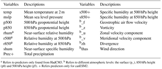
a Refers to predictors only found from HadCM3. b Refers to different atmospheric levels: the surface (p_), 850 hPa height (p8) and 500 hPa height (p5). + Refers predictors only for canESM2.
Moreover, atmospheric large-scale predictor variables used for representing the present condition were obtained from the National Centre for Environmental Prediction (NCEP) reanalysis data set. CanESM2, a second-generation Canadian earth system model (ESM) developed by Canadian Centre for Climate Modelling and Analysis (CCCma) of Environment Canada that represents CMIP5 and HadCM3 outputs from the Hadley Centre, United Kingdom (UK) representing CMIP3 were used in SDSM for the construction of daily local meteorological variables corresponding to their future climate scenario.
The reason for selecting these two GCMs was that they are models that made daily predictor variables freely available to be directly fed into the SDSM, covering the study area with a better resolution. Additionally, HadCM3 is the most-used GCM in previous studies such as Dibike et al. (2005), Dile et al. (2013), Hassan et al. (2014) and Yimer et al. (2009), and HadCM3 ranked first in performance evaluation done by MAGICC/SCEGEN computer program tools and its downscaled results match with the ensemble mean of the six GCMs used in the LARS-WG model. Furthermore, they can represent two different scenario generations describing the amount of greenhouse gases (GHGs) in the atmosphere in the future. HadCM3 GCM used emission scenarios of A2 (separated world scenario), in which the CO2 concentration was projected to be 414, 545 and 754 ppm, and B2 (the world of technological inequalities), where the CO2 concentration was expected to be 406, 486 and 581 ppm at the time periods of the 2020s, 2050s and 2080s respectively (Semenov and Stratonovitch, 2010) that were used in the CMIP3 for the IPCC's AR4 (IPCC, 2007). The canESM2 GCM represents the latest plausible radiative forcing scenarios, a wide range which includes a very low forcing level (RCP2.6), where radiative forcing peaks at approximately 3 W m−2, peaks approximately 490 ppm CO2 equivalent before 2100, and then declines to 2.6 W m−2; two medium stabilization scenarios were used for the IPCC's AR5, RCP6 and RCP 4.5, in which radiative forcing is stabilized at 6 W m−2 (approximately 850 ppm CO2 equivalent) and 4.5 W m−2 (approximately 650 ppm CO2 equivalent) after 2100 respectively, and one very high baseline emission scenario (RCP8.5) was used for which radiative forcing reaches > 8.5 W m−2 (1370 ppm CO2 equivalent) by 2100 and continues to rise for some time (IPCC, 2014).
The NCEP data set was normalized over the complete 1961–1990 period data, and interpolated to the same grid as HadCM3 (2.5∘ latitude × 3.75∘ longitude) and canESM2 (2.8125∘ latitude × 2.8125∘ longitude) from its horizontal resolution of (2.5∘ latitude × 2.5∘ longitude), to represent the current climate conditions. NCEP reanalysis data were normalized and interpolated as follows (Hassan et al., 2014):
in which un is the normalized atmospheric variable at time t, ut is the original data at time t, ua is the multiyear average during the period, and σu is the standard deviation.
The canESM2 outputs for three different climate scenarios are RCP 2.6, RCP 4.5 and RCP 8.5 for the period 2006–2100, while the outputs of HadCM3 for A2a (medium–high) and B2a (medium–low) emission scenarios for the period 1961–2099 were obtained on a grid-by-grid-box basis for the study area from the Environment Canada website http://ccds-dscc.ec.gc.ca/index.php?page=dst-sdi (the “a” in A2a and B2a refers the ensemble member in the HadCM3 A2 and B2 experiments). The archive of canESM2 and HadCM3 GCM output contains 26 daily predictor variables, each listed in Table 2.
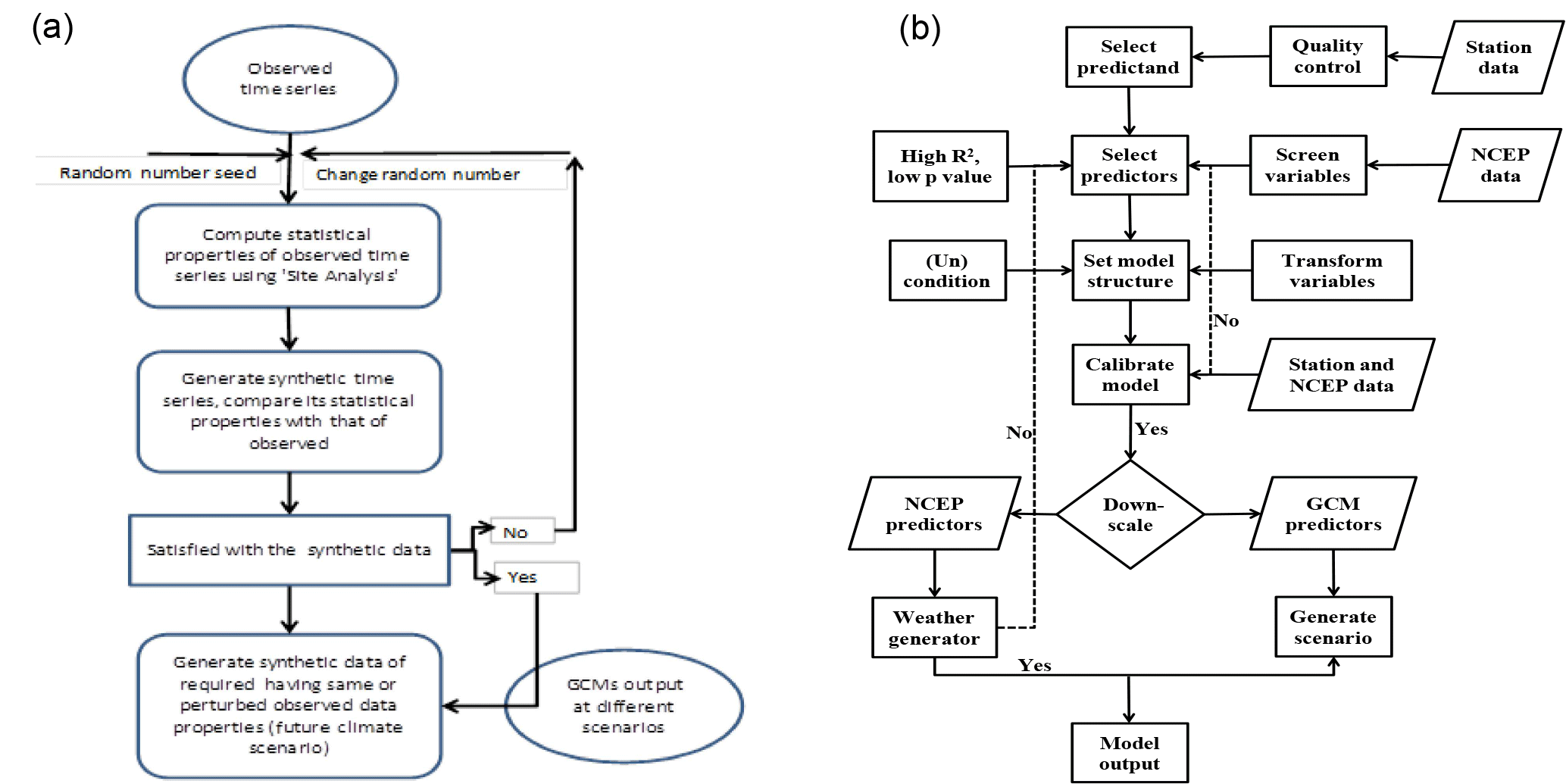
Figure 2Schematic diagram of (a) LARS WG analysis and (b) SDSM analysis. Source: Wilby et al. (2002).
4.1 Description of LARS-WG model
LARS-WG is a stochastic weather generator which can be used for the simulation of weather data at a single station under both current and future climate conditions. These data are in the form of daily time series for a group of climate variables, namely precipitation, maximum temperature and minimum temperature, and solar radiation (Chen et al., 2013; Semenov et al., 1997). LARS-WG uses a semiempirical distribution (SED) that is defined as the cumulative probability distribution function (CDF) to approximate probability distributions of dry and wet series, daily precipitation, minimum temperatures and maximum temperatures.
EPM is a histogram of the distribution of 23 different intervals (ai−1, ai) where ai−1 < ai (Semenov et al., 2002), which offers a more accurate representation of the observed distribution compared with the 10 used in the previous version. By perturbing parameters of distributions for a site with the predicted changes of climate derived from global or regional climate models, a daily climate scenario for this site could be generated and used in conjunction with a process-based impact model for assessment of impacts. In general, the process of generating synthetic weather data can be categorized into three distinct steps: model calibration, model validation and scenario generation as represented in Fig. 2a, which are briefly described by (Semenov et al., 2002) as follows.
The inputs to LARS-WG are the series of daily observed data (precipitation, minimum temperature and maximum temperature) of the base period (1984–2011) and site information (latitude, longitude and altitude). After the input data preparation and quality control, the observed daily weather data at a given site were used to determine a set of parameters for probability distributions of weather variables. These parameters are used to generate a synthetic weather time series of arbitrary length by randomly selecting values from the appropriate distributions, with the same statistical characteristics as the original observed data but differing on a day-to-day basis. The LARS-WG distinguishes wet days from dry days based on whether the precipitation is greater than zero. The occurrence of precipitation is modeled by alternating wet and dry series approximated by semiempirical probability distributions. The statistical characteristics of the observed and synthetic weather data during calibration of the model are analyzed to determine if there are any statistically significant differences using a chi-square goodness-of-fit test (Kolmogorov–Smirnov, KS) and the means and standard deviation using t and F test respectively. This can be done by changing the parameters of LARS-WG (number of years and seed number).
To generate climate scenarios at a site for a certain future period with a selected emission scenario, the LARS-WG baseline parameters, which are calculated from observed weather for a baseline period (1984–2011), are adjusted by the Δ-changes for the future period and the emissions predicted by a GCM for each climatic variable for the grid covering the site. In this study, the local-scale climate scenarios based on the SRES A2, A1B and B1 scenarios simulated by the selected six GCMs are generated for the time periods of 2011–2030, 2046–2065 and 2080–2099 to predict the future change of precipitation and temperature in UBNRB.
Δ-changes were calculated as relative changes for precipitation and absolute changes for minimum and maximum temperatures (Eqs. 3 and 3) respectively. No adjustments for distributions of dry and wet series and temperature variability were made, because this would require daily output from the GCMs which is not readily available from the LARS-WG data set (Semenov et al., 2010).
In the above equations, ΔTi and ΔPi are climate change scenarios of the temperature and precipitation, respectively, for long-term averages for each month (); and are the long-term average temperature and precipitation respectively, simulated by the GCM in the future periods per month for three time periods, and are the long-term average temperature and precipitation respectively, simulated by the model in the period similar to observation period (in this study 1984–2011) for each month. For obtaining time series of future climate scenarios, climate change scenarios are added to the observed values by employing the change factor (CF) method (Eqs. 3 and 3) (in this study 1984–2011).
T and P are time series of the future climate scenarios of temperature and precipitation (2011–2100), and Tobs and Pobs are observed temperature and precipitation. So, in LARS-WG downscaling, unlike in SDSM, large-scale atmospheric variables are not directly used in the model, but rather are based on the relative mean monthly changes between current and future periods predicted by a GCM. Local station climate variables are adjusted proportionately to represent climate change (Dibike et al., 2005).
4.2 Description of SDSM
The SDSM is best described as a hybrid of the stochastic weather generator and regression based on the family of transfer function methods, due to the fact that a multiple linear regression model is developed between a few selected large-scale predictor variables (Table 2) and local-scale predictands such as temperature and precipitation in order to condition local-scale weather parameters from large-scale circulation patterns. The stochastic component of SDSM enables the generation of multiple simulations with slightly different time series attributes, but the same overall statistical properties (Wilby et al., 2002). It requires two types of daily data: the first type corresponds to local predictands of interest (e.g., temperature, precipitation) and the second type corresponds to the data of large-scale predictors (NCEP and GCM) of a grid box closest to the station.
The SDSM model categorizes the task of downscaling into a series of discrete processes such as quality control and data transformation, screening of predictor variables, model calibration, and weather and scenario generation as shown in Fig. 2b. Detail procedures and steps can be found in Wilby et al. (2002) for further reading. Screening potentially useful predictor–predictand relationships for model calibration is one of the most challenging but very crucial stages in the development of any statistical downscaling model. It is because of the fact that the selection of appropriate predictor variables largely determines the success of SDSM and also the character of the downscaled climate scenario (Wilby et al., 2007). After routine screening procedures, the predictor variables that provide physically sensible meaning in terms of their high explained variance, correlation coefficient (r) and the magnitude of their probability (p value) were selected.
The model calibration process in SDSM was used to construct downscaled data based on multiple regression equations given daily weather data (predictand) and the selected predictor variables at each station. The model was structured as a monthly model for both daily precipitation and temperature using the same set of the selected NCEP predictors for the calibration period. Hence, 12 regression equations were developed for 12 months. Bias correction and variance inflation factor were adjusted until the model replicated the observed data. Model validation was carried out by testing the model using an independent data set. To compare the observed and simulated data, SDSM has provided a summary statistics function that summarizes the result of both the observed and simulated data. Time series of station data and large-scale predictor variables (NCEP reanalysis data) were divided into two groups: for the periods 1984–1995 (1984–2000) and 1996–2001 (2001–2005) for model calibration and validation of HadCM3 (canESM2) GCMs.
The scenario generator operation produces ensembles of synthetic daily weather series given observed daily atmospheric predictor variables supplied by a GCM for either current or future climates (Wilby et al., 2002). The scenario generation produced 20 ensemble members of synthetic weather data for 139 years (1961–2099) from HadCM3 A2a and B2a scenarios and for 95 years (2006–2100) from canESM2 for RCP2.6, 4.5 and 8.5 scenarios, and the mean of the ensemble members was calculated and used for further climate change analysis. The generated scenario was divided into three time windows of 30 years of data: 2011–2040, 2041–2070 and 2071–2100.
4.3 Downscaling model performance evaluation criteria
A number of statistical tests were carried out to compare the skills of the two downscaling models categorized into two main classes. First, quantitative statistical tests using metrics, such as mean absolute error (MAE), root mean square error and bias. These metrics are by far the most widely used and accepted of the many possible numerical metrics (Amirabadizadeh et al., 2016; Bennett et al., 2013) to evaluate the comparative performance of the models to simulate the current climate variable of precipitation on the basis of long-term monthly averages defined by using Eqs. (3)–(3). In this study correlation and correlation-based measures such as coefficient of determination (R2) and coefficient of efficiency (Nash–Sutcliffe efficiency, NSE) are not included due to the fact that these measures are oversensitive to extreme values and are insensitive to additive and proportional differences between model simulations and observations (Legates and McCabe, 1999). Evaluation was done in two steps as suggested by Goly et al. (2014): (i) equally weighing the metrics and (ii) varying the weights of metrics. For the case of equally weighted the following steps were applied. (a) Comparison of the values of the performance metrics among the models and ranking (obtaining individual model rankings for each performance metrics) at station level. Here, score 1 will be given to the model that has smaller metrics value and score 3 to the one having larger value and 2 for the model having the value in between. (b) Summing up the score pertaining to each model across all the stations. (c) Once the final scores are obtained for each evaluation metric, the models are ranked again based on the totals by summing up the metrics score value for each models.
In the above equations Xi and Yi are the ith observation and simulated data by the model, respectively, μx and μy are the average of all data of Xi and Yi in the study population, and n is the number of all samples to be tested.
Additionally, the varying weights technique was applied to the performance metrics as given in Eq. (3) to rank the models according to their skills. To avoid the discrepancy in weighing the performance measures because of differences in the order of their magnitudes, each performance measure is normalized (divided by the maximum value) and then the cumulative weighted performance measure for each downscaling model is calculated (Goly et al., 2014). The weights of metrics are arranged in such a way that more emphasis is given to MAE and RMSE, followed by bias (0.5, 0.35 and 0.15 respectively).
where the index i refers to a downscaling model, Wi refers to overall performance measure, and .
Secondly, qualitative tests, comparing the skill of models in regard to capturing the distribution of the observed data to the whole range and in capturing the extreme precipitation events. For this purpose, statistical metrics such as IRF, ABC, 99p, 95p, 1daymax, R1, R10, R20 and SDII and graphical representations of box–whisker plots and KS cumulative distribution test were applied. KS is used to compare the probability distribution function (PDF) of the observations to the PDF of the simulated precipitation (Simard and L'Ecuyer, 2011). These plots provide a convenient visual summary of several statistical properties of the data set as they vary over time. A scoring technique is applied to compare the accuracy of the models. In this scoring technique, the bias of an evaluation metric for each station is used: score 1 will be given to the model that has smaller bias, score 3 to the one with a larger bias and 2 for the model with a value in between. Afterwards, evaluation was carried out using an equally weighted method only due to the assumption that the metrics have equal weights, as discussed above for model ranking. For the Kolmogorov–Smirnov cumulative distribution test, the observed and the simulated precipitation data from each model were compared using a p value at the significance level of 5 % for each station. The computed p value is lower than the significance level α = 0.05, which indicates the simulated fail to follow the same distribution as the observed. Furthermore, the F test and t test are applied to test the equality of monthly variances of precipitation and equality of monthly mean respectively.
Table 3Calibration results of the average statistical tests comparing the observed data from 26 stations with synthetic data generated through LARS-WG. The numbers in the table show the average numbers of tests gave a p value of less than 5 % significance level.
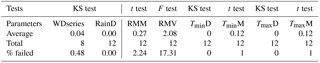
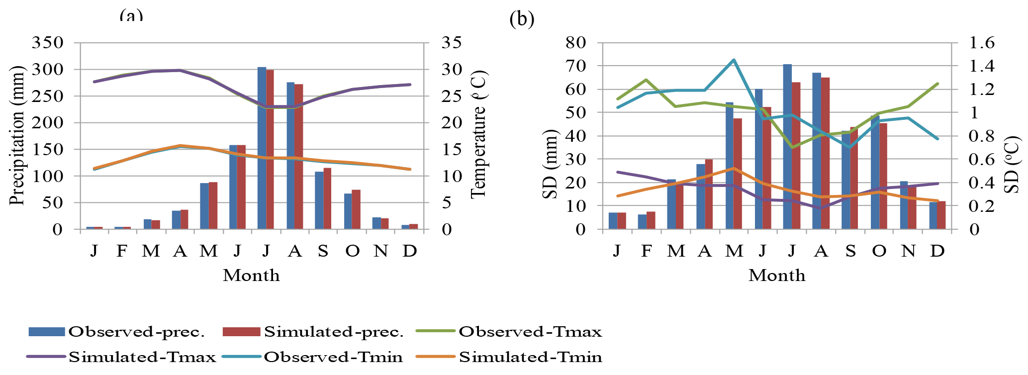
Figure 3Observed and simulated (a) mean monthly precipitation, Tmax and Tmin; (b) standard deviation of precipitation, Tmax and Tmin using LARS-WG.
IRF and ABC are recommended by Campozano et al. (2016), while 95p, 99p, 1day max, R1, R10, R20 and SDII are recommended by Expert on Climate Change Detection and Indices (ETCCDI). The interquartile relative fraction (IRF): to evaluate the modeled variability representation relative to the observed is defined by Eq. (3):
where and are the 75th modeled and observed percentile, and and are the 25th modeled and observed percentile respectively. A value of IRF > 1 represents overestimation of the variability, IRF = 1 is a perfect representation of the variability, and IRF < 1 is an underestimation of the variability. To evaluate the bias of the 25th, 50th and 75th percentiles, the absolute cumulative bias (ACB) is defined as Eq. (4):
where and are the 75th modeled and observed percentile, and are the 50th modeled and observed percentile , and are the 25th modeled and observed percentile respectively. A value of ACB = 0 is a perfect representation of the modeled and observed distributions, while under- or overestimation indicates a divergence of ACB from zero to positive values. The terms 95p and 99p denote the 95th and 99th percentiles of daily precipitation amount respectively; 1 daymax is the highest 1-day precipitation amount; R1, R10 and R20 are number of precipitation days (≥ 1 mm), heavy precipitation days (≥ 10 mm) and extreme heavy precipitation days ≥ 20 mm respectively; and SDII is the simple daily intensity index calculated as the ratio of total precipitation to the number of wet days (≥ 1 mm).
5.1 Calibration and validation of LARS-WG
To verify the performance of LARS-WG, in addition to the graphic comparison, some statistical tests were performed. The KS test is performed to test equality of the seasonal distributions of wet and dry series (WDSeries), distributions of daily rainfall (RainD), and distributions of daily maximum (TmaxD) and minimum (TminD) temperature. The F test is performed to test equality of monthly variances of precipitation (RMV) while the t test is performed to verify equality of monthly mean rainfall (RMM), monthly mean of daily maximum temperature (TmaxM), and monthly mean of daily minimum temperature (TminM). All of the tests calculate a p value, which is used to accept or reject the hypotheses that the two sets of data (observed and generated) could have come from the same distribution at the 5 % significance level. Therefore, the average number of p values less than 5 % recorded from 26 stations and the percentage that failed from the total of 8 seasons or 12 months have been presented in Table 3. The result revealed that LARS-WG performs very well for all parameters except RMM and RMV. However, an average of 2.2 and 17.3 % of the months of a year obtained a p value < 5 % for the monthly mean and variance of precipitation respectively. From these numbers, it can be noted that the model is less capable of simulating the monthly variances than the other parameters.
For illustrative purposes, a graphical representation of monthly mean and standard deviation of the simulated and observed precipitation, Tmax and Tmin, was constructed (see Fig. 3) for the randomly chosen Gondar station as it has been difficult to present the result of all stations. It can be seen from the result that observed and simulated monthly mean precipitation, Tmax and Tmin, match very well. However, as it is known to be difficult to simulate the standard deviations in most statistical downscaling studies, the performance of the standard deviation is less accurate compared to the mean (Fig. 3b).

Figure 4(a) Relative change mean annual precipitation and (b) change in Tmax and Tmin modeled from six GCMs for three time periods of UBNRB compared from the reference period of 1984–2011 by using LARS-WG.
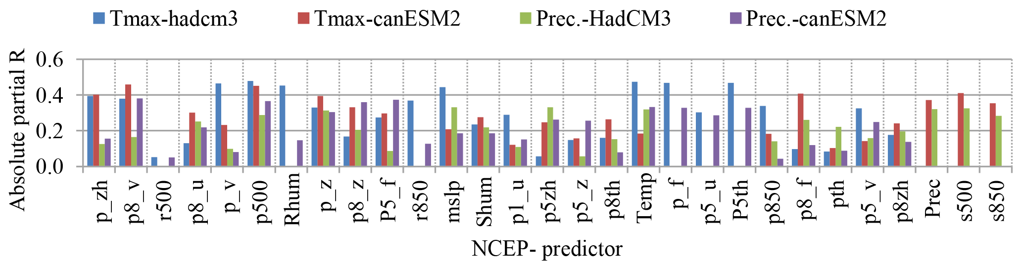
Figure 5Average partial correlation coefficient values of all stations for precipitation and Tmax with NCEP predictors.
5.2 Screening variable, model calibration and validation of SDSM
Initially, offline correlation analysis was performed using SPSS software between predictands and NCEP reanalysis predictors to identify an optimal lag and physically sensible predictors for climate variables of precipitation, Tmax and Tmin. Analysis of the offline correlation revealed that an optimal lag or time shift does not improve the correlation of predictands and predictors for this particular study. Average partial correlation of observed precipitation with predictors as shown in Fig. 5 indicates all stations followed the same correlation pattern (both in magnitude and direction) that illustrates all stations can have identical physically sensible predictors, with a few exceptions. Furthermore, there are a number of predictors that have correlation coefficient values in the range of 20 to 45 % for precipitation across all stations. This range is considered to be acceptable when dealing with precipitation downscaling (Wilby et al., 2002) because of its complexity and high spatial and temporal variability to downscale.
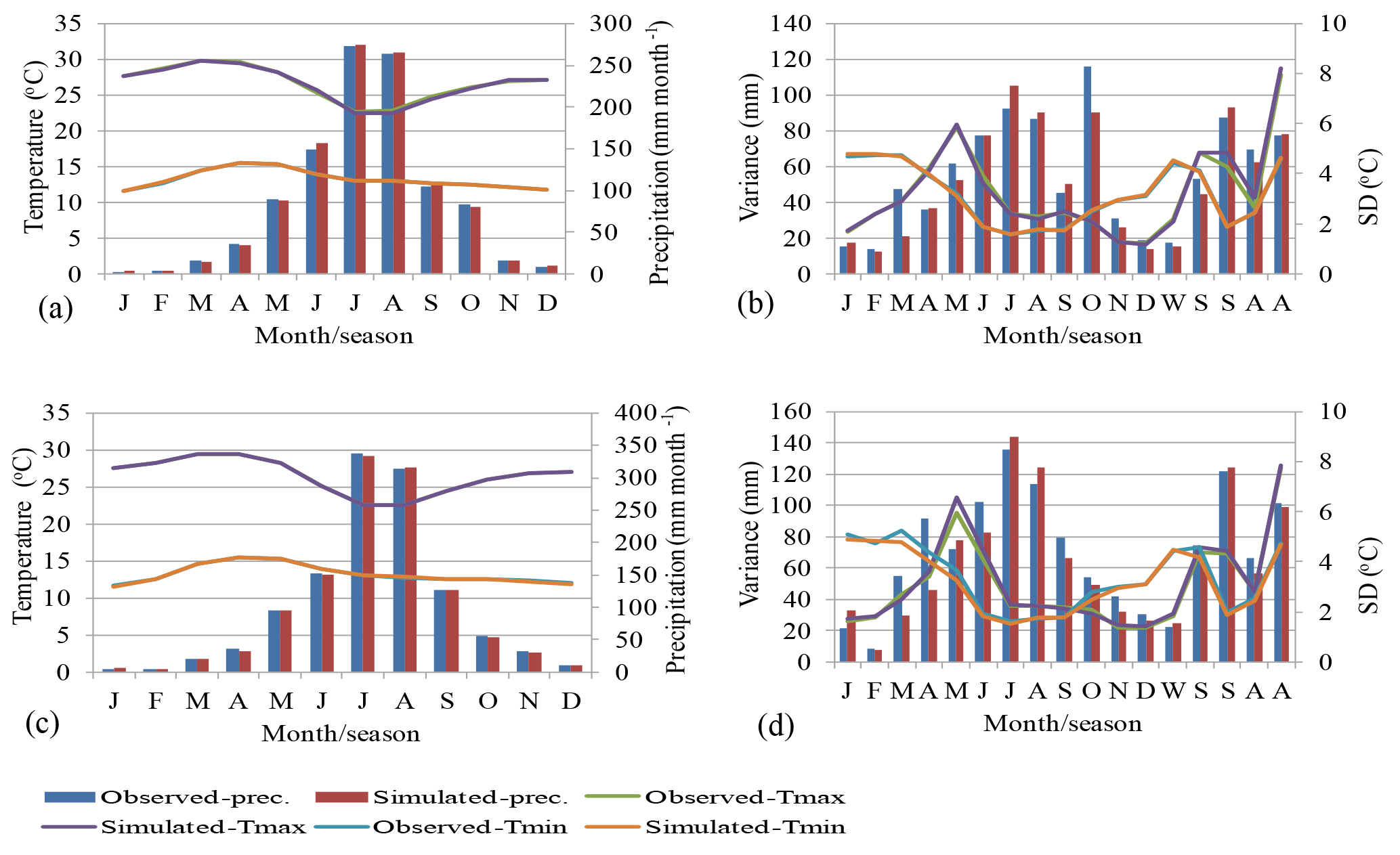
Figure 6Calibration of observed and simulated of precipitation, maximum temperature and minimum temperature for the Gondar station using SDSM from canESM2 and HadCM3 from (a, b) to (c, d).
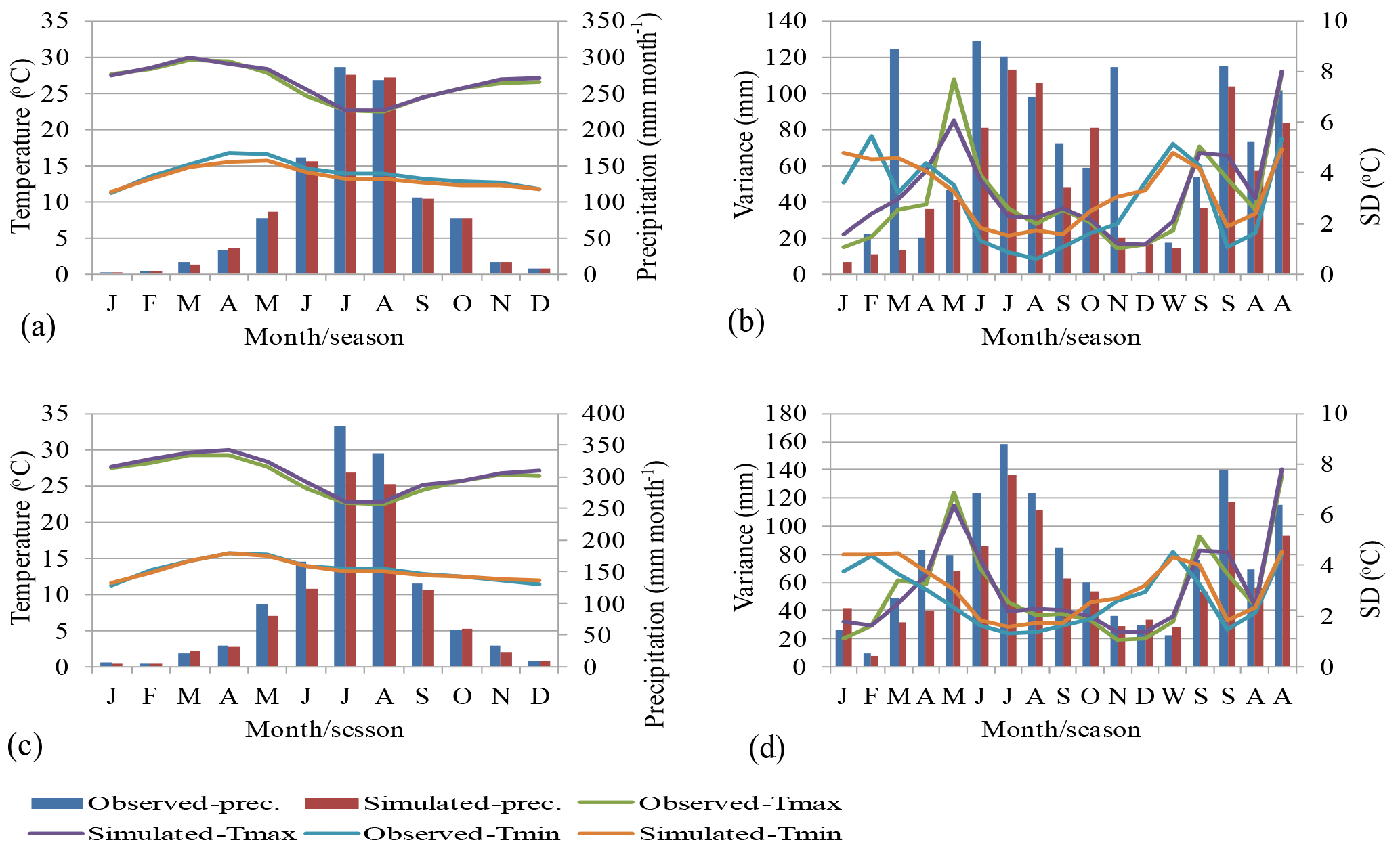
Figure 7Validation of observed and simulated of precipitation, maximum temperature and minimum temperature for Gondar station using SDSM from canESM2 and HadCM3 from(a, b) to (c, d) respectively.

Figure 8(a) Relative change of mean annual precipitation, and (b) change of mean annual Tmax and Tmin for three time periods compared to the baseline period of UBNRB using SDSM for HadCM3 and canESM2 GCMs under different scenarios.
The predictor variables identified for each downscaling GCM and for the corresponding local climate variables showed that different large-scale atmospheric variables control different local variables. For instance, the set of temp, mslp, s500, s850, p8_v, p500, shum comprises the most potential or meaningful predictors for temperature, and the set of s500, s850, p8_u, p_z, pzh, p500 performs best for predicting precipitation of the study area, which is consistent with the result of offline correlation analysis. After carefully screening predictor variables, model calibration and validation was carried out. The graphical comparison between the observed and generated rainfall, Tmax and Tmin, was run to enhance the confidence of the model performance, as shown in Figs. 6 and 7 for Gondar station only. Examination of Fig. 6 shows that the calibrated model reproduces the monthly mean precipitation and mean standard deviation of daily Tmax and Tmin values quite well. However, the model is less accurate in reproducing variance of observed precipitation. As Wilby et al. (2004) point out, downscaling models are often regarded as less able to model the variance of the observed precipitation with great accuracy.
The statistical performance metrics of MAE and RMSE values for the monthly precipitation modeled from canESM2 range from 3.5 to 14.8 mm and 4.9 to 22.4 mm, which shows that canESM2 performs better than HadCM3, with the MAE and RMSE values ranging from 6.2 to 48.6 mm and 7.6 to 73.4 mm respectively. The result of statistical analysis revealed that the model is much better in simulating Tmax and Tmin than precipitation, because the high dynamical properties of precipitation make it difficult to simulate. After accomplishing a satisfactory calibration, the multiple regression model is validated using an independent set of data outside the period for which the model is calibrated. The validation result revealed that the model is successfully validated but with less accuracy compared to calibration for both GCMs as shown in Fig. 7. In general, the result analysis of performance measure and graphical representation of observed and simulated scenarios, both for calibration and validation, revealed that the model performs very well in simulating the climate variables.
5.3 Downscaling with LARS-WG
Since the performance of LARS-WG during calibration and validation was very good, downscaling of the climate scenario can be done from six selected multimodel CMIP3 GCMs under three scenarios (A1B, B1 and A2) for three time periods. After downscaling the future climate scenarios at all stations from the selected six GCMs, the projected precipitation analysis for the areal UBNRB was calculated from the point rainfall stations using the Thiessen polygon method. The result analysis (Fig. 4a) revealed that GCMs disagree on the direction of precipitation change: two GCMs (CSMK3 and GFCM21) showed decreasing trends, and a majority, or four, GCMs (NCCSM, Hadcm3, MPEH5 and MIHR) showed increasing trends from the reference period in all three time periods. By the 2030s, the relative change in mean annual precipitation is projected in the range between −2.3 and 6.5 % for A1B, −2.3 and 7.8 % for B1, and −3.7 and 6.4 % for A2 emission scenarios. In the 2050s, the relative changes in precipitation range between −8 and 22.7 % for A1B, −2.7 and 22 % for B1, and −7.4 and 8.7 % for A2 scenarios. In the time of 2080s, the relative changes in precipitation projected may vary between −7.5 and 29.9 % for A1B, −5.3 and 13.7 % for B1, and −5.9 and 43.8 % for A2 emission scenarios. The multimodel average result showed that in the future precipitation may generally increase over the basin in the range of 1 to 14.4 %, which is in line with the result from the HadCM3 GCM (0.8 to 16.6 %).
In a different way from precipitation, the projections of mean annual Tmax and Tmin have showed coherent increasing trends from the six GCMs under all scenarios in all three future time periods (Fig. 4b). The result calculated from the ensemble mean showed that mean annual Tmax may increase up to 0.5, 1.8 and 3.6 ∘C by 2030s, 2050s and 2080s respectively under the A2 scenario, which is in line with the results from both GFCM21 and HadCM3 GCMs. Likewise, the UBNRB may experience an increase in mean annual Tmin up to 0.6, 1.8 and 3.6 ∘C by the 2030s, 2050s and 2080s respectively from the multimodel average.
Table 4Performance measure and ranking of models during the baseline period (1984–2011) for evaluation metric RMSE.
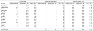
Table 5Statistical downscaling models ranking during the baseline period (1984–2011) for quantitative measures. The numbers in the table show the total ranking scores summed up from 15 stations.
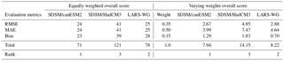
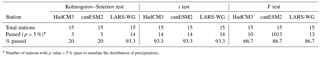
Table 6Ranking of statistical downscaling models during the baseline period (1984–2011) for qualitative measures (distribution and extreme events of daily precipitation). The numbers in the table show the total ranking scores obtained from 15 stations.
5.4 Downscaling with SDSM
Here, as it is difficult to process all the selected six CMIP3 GCM3 using SDSM, we choose the HadCM3 GCM as the best due to the fact that the downscaling result of HadCM3 using LARS-WG fits with the downscaling result of the ensemble mean model. Also, canESM2 from the CMIP5 GCMs was selected to test the improvements of CMIP5 over CMIP3. Results of downscaling future climate scenario of areal UBNRB using SDSM calculated from all stations using Thiessen polygon methods are summarized in Fig. 8. The overall analysis of the result indicates a general increase in mean annual precipitation for three time windows (2030s, 2050s and 2080s) for all five scenarios (A2a and B2a for HadCM3 and RCP2.6, RCP4.5 and RCP8.5 for canESM2) in the range of 2.1 to 43.8 %. The maximum (minimum) relative change of mean annual precipitation is projected to be 43.8 % (6.2 %), 29.5 % (3.5 %) and 19 % (2.1 %) in the 2080s, 2050s and 2030s under the RCP8.5 scenario of canESM2 (B2a) scenario of HadCM3. In general, the RCP8.5 scenario of canESM2GCM resulted in pronounced increases in all three time periods, whereas scenario B2a of the HadCM3 GCM reported minimum change over the study area.
Regarding temperature, the downscaling result of Tmax and Tmin showed an increasing trend consistently in all months and seasons in three time periods under all scenarios with mean annual value ranging from 0.5 to 2.6 ∘C and 0.3 to 1.6 ∘C under scenario RCP8.5 and B2a respectively. The RCP 8.5 scenario reported maximum change while B2a scenario reported minimum change both for Tmax and Tmin in all three time periods compared to other scenarios. The analysis of the downscaling result illustrates maximum temperature may become much hotter compared to minimum temperature in all scenarios and time periods in the future across the UBNRB.
5.5 Comparative performance evaluation of LARS-WG and SDSM models
Chen et al. (2013) argued that though major sources of uncertainty are linked to GCMs and emission scenarios, uncertainty related to the choice of downscaling methods give less attention to climate change analysis. Therefore, in this study, comparative performance evaluation of the downscaling methods has been given due emphasis and carried out in a number of statistical and graphical tests both quantitatively and qualitatively. The model skill was evaluated and ranked at each site for each metric as shown in Table 4 for metrics of RMSE. The overall rank obtained by summing up the score of each model for each metric is presented in Tables 5 and 6, for quantitative and qualitative measures respectively.
The result revealed that SDSM/canESM2 narrowly performed best in simulating the long-term average values in both equally weighted and varying weights of the quantitative metrics. However, LARS-WG performed best in qualitative measures in reproducing the distribution and extreme events of daily precipitation. For instance, absolute bias for the 95th percentile of daily precipitation (95p) ranges from 4.35 to 12.4 mm for SDSM/canESM2, from 3.2 to 12.2 mm for SDSM/HadCM3 and from 0.07 to 3.7 mm for LARS-WG; for the mean of daily precipitation amount (SDII), absolute bias ranges from 1.3 to 6.3 mm for SDSM/canESM2, from 2.1 to 5.6 mm for SDSM/HadCM3 and from 0.01 to 3 mm for LARS-WG.
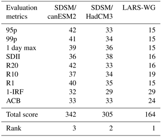
Table 7Kolmogorov–Smirnov, t and F tests during the baseline period (1984–2011) for qualitative measures.
* Number of stations with p value > 5 % (pass to simulate the distribution of precipitation).
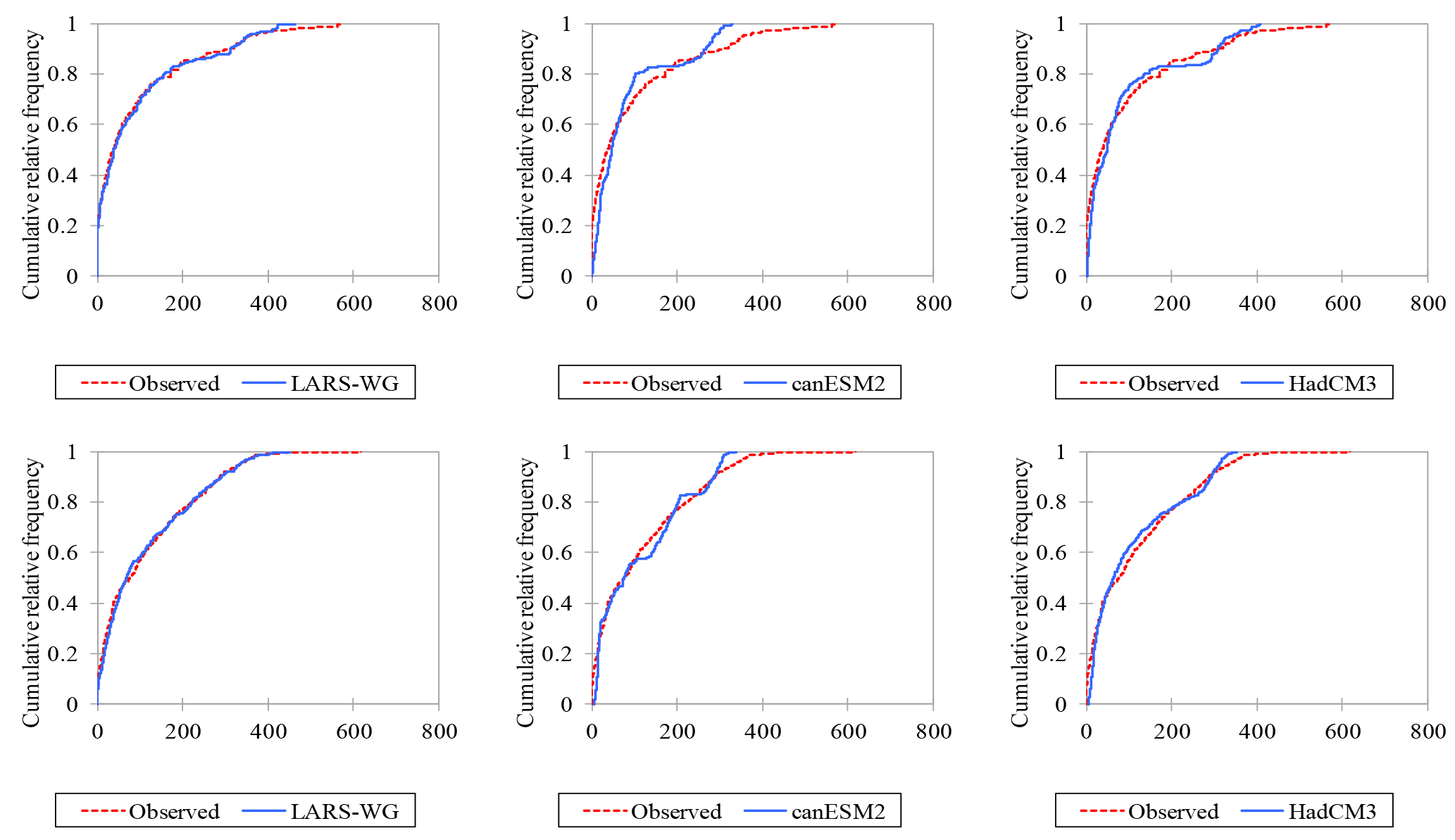
Figure 9Kolmogorov–Smirnov test to compare the skill of the models for the observed precipitation distribution (upper three Alemketema stations, lower three Debre Markos stations).
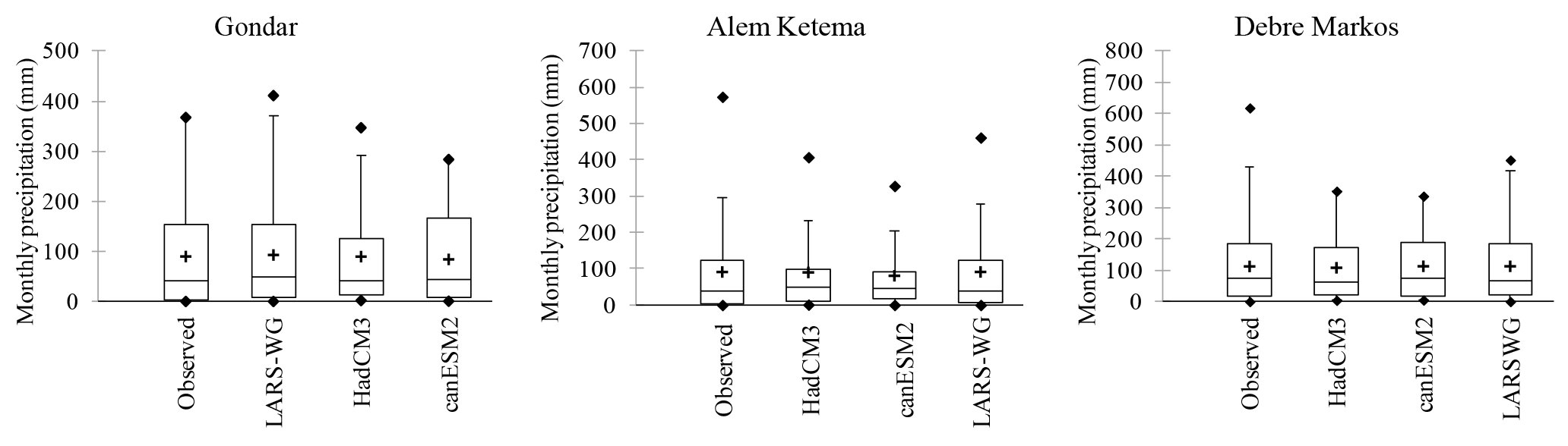
Figure 10Box plot showing the model performance for three stations on a monthly basis. Box boundaries indicate the 25th and 75th percentiles, the line within the box marks the median, whiskers below and above the box indicate the 10th and 90th percentiles, and dots indicate the extremes.
Furthermore, as the Kolmogorov–Smirnov test from Table 7 shows, LARS-WG captures the distribution of the observed precipitation of 93.3 % from all stations while SDSM captures only 20 % of the 15 stations equally both from canESM2 and HadCM3 GCMs at 5 % significance level. The t test result revealed that 86.7 % of the simulated precipitation by LARS-WG and SDSM/HadCM3 models are capturing their perspective mean values from all stations while the SDSM and hadCM3 models capture only 66.7 %. The F test showed 93.3 % of the simulated and the observed precipitation are normally distributed around their respective variance value in all three models. In general, the comparative performance test revealed that the LARS-WG model performed best in qualitative measures while SDSM/canESM2 is best in quantitative measures in UBNRB. In addition, Figs. 9 and 10 confirmed graphically the ability of the LARS-WG model in capturing the distribution and extreme events of the precipitation in representative stations (randomly chosen) by a whisker box plot and Kolmogorov–Smirnov test respectively.
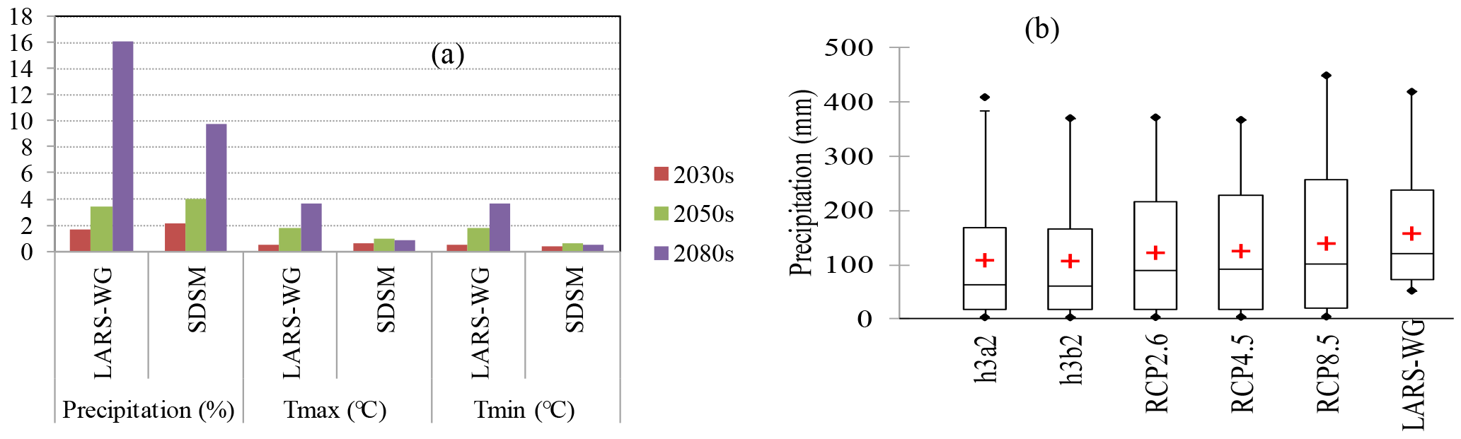
Figure 11Comparison of climate change scenarios (a) downscaled using LARS-WG and SDSM from HadCM3 GCM for the a2 scenario and (b) downscaled from different scenarios (LARS-WG using hadCM3 a2 scenario).
For future simulation, the HadCM3 GCM A2 scenario was used in common for two (LARS-WG and SDSM) downscaling methods to test whether the downscaling methods may affect the GCM result under the same forcing scenario. The results obtained from the two downscaling models were found reasonably comparable and both approaches showed increasing trends for precipitation, Tmax and Tmin. However, the magnitude of the downscaled climate data from the two methods as presented in Fig. 11 indicates that LARS-WG overpredicts precipitation and temperature compared to SDSM. The relative change of mean annual precipitation using LARS-WG is about 16.1 % and an average increase in mean annual Tmax and Tmin is about 3.7 and 3.6 ∘C respectively in the 2080s. SDSM predicts the relative change of mean annual precipitation of only about 9.7 % and an average increase in Tmax and Tmin of about 2 and 1.3 ∘C respectively in the same period. The differences in the future predictions are the result of the differences in the basic concepts behind the two downscaling techniques. The SDSM uses large-scale predictor variables from GCM outputs which can be considered as more reliable for climate change prediction using multiple linear regression. However, the LARS WG uses the relative change factors (RCFs) derived from the direct GCM output of only those variables which directly correspond to the predictands. Hence, because of the well-known fact that GCMs are not very reliable in simulating precipitation, the error induced from the GCM output for precipitation will propagate the error of downscaling that makes the performance of LARS-WG to downscale precipitation needs more caution (Dibike et al., 2005).
The uncertainty related to climate change analysis can be due to climate models and downscaling methods among many other factors. In this study, we employed a multimodel approach to see that the uncertainties came from different GCMs. In total, 21 systematically selected future climate scenarios were produced for each time period, which we might think representative to understand fully and to project plausibly the future climate change in the study area and to retain information about the full variability of GCMs. Moreover, we applied two widely used statistical downscaling methods, namely the regression downscaling technique (SDSM) and the stochastic weather generation method (LARS WG) for this particular study.
The performance of the three models (HadCM3/SDSM, canESM2/SDSM and LARS-WG) were tested for the baseline period of 1984–2011 in representing the current situation, particularly for precipitation, as it is the most difficult climate variable to model. The result suggested that SDSM using canESM2 GCM captures the long-term monthly average very well at most of the stations and it ranked first from others. This could be attributed to the increasing performance of GCMs from time to time (i.e., CMIP5 GCMs performs better than CMIP3 GCMs) due to the fact that modeling was based on the new set of radiative forcing scenarios that replaced SRES emission scenarios, constructed for IPCC AR5 where the impacts of land use and land cover change on the environment and climate are explicitly included. However, LARS-WG performed best in qualitative measures in capturing the distribution and extreme events of the daily precipitation than SDSM. The better performance of LARS-WG in capturing the distribution and extreme events of the daily precipitation may be associated with the use of 23 interval histograms for the construction of semiempirical distribution, which offers a more accurate representation of the observed distribution compared with the 10 intervals used in the previous version (Semenov et al., 2010). The poor performance of SDSM would indicate the difficulty in finding climate variables from the NCEP data that could explain the variability of daily precipitation well. Therefore, LARS-WG would be more preferred in areas of the UBNRB where there is high climatic variability to correctly simulate the distribution and extreme events of the precipitation, which is crucial for a realistic assessment of flood events and agricultural production.
The downscaling result reported from the six GCMs used in LARS-WG showed large intermodel differences: two GCMs reported that precipitation may decrease while four GCMs reported that precipitation may increase in the future. The large intermodel differences in the GCMs showed the uncertainties of GCMs associated with their differences of resolution and assumptions of physical atmospheric processes to represent local-scale climate variables, which are typical characteristics for Africa and because of low convergence in climate model projections in the area of UBNRB (Gebre and Ludwig, 2015). These results further reinforce multimodel strategies for conducting climate change studies. The multimodel average result showed that in the future precipitation may generally increase over the basin in the range of 1 to 14.4 % which is in line with the result from HadCM3 GCM (0.8 to 16.6 %); this indicates that HadCM3 from CMIP3 GCMs has a better representation of local-scale climate variables in the study area, consistent with the previous study result by Kim and Kaluarachchi (2009) and Dile et al. (2013) in the same study area.
LARS-WG produces synthetic climate data of any length with the same characteristics as the input record, and it simulates weather separately for a single site. Therefore, the resulting weather series for different sites are independent of each other, which can cause loss of a very strong spatial correlation that exists in real weather data during simulation. However, a few stochastic models have been developed to produce weather series simultaneously at multiple sites, preserving the spatial correlation, mainly for daily precipitation, such as space–time models, nonhomogeneous hidden Markov models and nonparametric models that typically use a K nearest-neighbor (K-NN) procedure (King et al., 2015). They are complicated in both calibration and implementation and are unable to adequately reproduce the observed correlations (Khalili et al., 2007). In this study, the simple Pearson's correlation coefficient (R2) value was checked in two stations before and after simulation of the observed data to test the capability of LARS-WG in preserving the spatial correlation of stations. The result revealed that the spatial correlation of the stations distorted or decreased from the original is insignificant.
In conclusion, a multimodel average from LARS-WG and individual model result from SDSM showed a general increasing trend for all three climatic variables (precipitation, Tmax and Tmin) in all three time periods. The positive change in precipitation in future can be a good opportunity for the farmers who are engaged in rainfed agriculture to maximize their agricultural production and to change their livelihoods. However, this information cannot be a guarantee for irrigation farming because precipitation is not the only factor affecting the flow of the river, which is the main source for irrigation. Evapotranspiration, dynamics of land use land cover, proper water resource management and other climatic factors which are not yet assessed by this study can influence the flow of the river directly and indirectly. Furthermore, the result from this study revealed that maximum positive precipitation change may occur in Autumn (September–November), when most agricultural crops mature and harvesting begins, while minimum precipitation change may occur during summer (June–August), when about 80 % of the annual rainfall occurs; this climate variability can be a potential threat to the farmers, who have limited ability to cope with the negative impacts of climate variability and overall ongoing economic development efforts in the basin.
In general, this study has shown that climate change will likely occur that may affect the water resources and hydrology of the UBNRB. On the basis of the results obtained in this study, both SDSM and LARS-WG models can be adopted with reasonable confidence as downscaling tools to undertake climate change impact assessment studies for the future. However, LARS-WG is more suitable for extreme precipitation impact assessment studies, such as those dealing with floods and droughts. Moreover, the paper provides substantial information that the choice of downscaling methods has a contribution in the uncertainty of future climate prediction. The authors would also like to suggest further assessment of the study area using a large ensemble of CMIP5 GCMs. Further relative performance of downscaling techniques for other climatic variables such as Tmax, Tmin, dry spell length, wet spell length, inter-annual and seasonal cycle of precipitation using additional PDF-based metrics such as the Brier score and the skill score might counteract the limitations of this paper.
The data can be made available upon request to the corresponding author.
The authors declare that they have no conflict of interest.
We are grateful to the Ethiopian Meteorological Agency (EMA) for providing us
the meteorological data for free. The first author received financial support
for traveling money from the DAAD water–food–energy NeXus project. The
authors are indebted to the two anonymous reviewers and the editor, Dimitri
Solomatine, for their critique and constructive suggestions and comments on
earlier versions of this paper, which were helpful in the improvement of the
manuscript.
This work was supported by the
German Research
Foundation (DFG) and the Technische
Universität
München within the funding programme
Open Access Publishing.
Edited
by: Dimitri Solomatine
Reviewed by: two anonymous referees
Amirabadizadeh, M., Ghazali, A. H., Huang, Y. F., and Wayayok, A.: Downscaling daily precipitation and temperatures over the Langat River Basin in Malaysia: a comparison of two statistical downscaling approaches, International Journal of Water Resources and Environmental Engineering, 8, 120–136, 2016.
Awulachew, S. B., Yilma, A. D., Loulseged, M., Loiskandl, W., Ayana, M., and Alamirew, T.: Water Resources and Irrigation Development in Ethiopia, Working Paper 123, International Water Management Institute, Colombo, Sri Lanka, 78 pp., 2007.
BCEOM: Abbay River Basin Integrated Development Master Plan, section II, volume V – Water Resources Development, part 1 – Irrigation and Drainage, Ministry of Water Resources, Addis Ababa, Ethiopia, 1998.
Bennett, N. D., Croke, B. F., Guariso, G., Guillaume, J. H., Hamilton, S. H., Jakeman, A. J., Marsili-Libelli, S., Newham, L. T., Norton, J. P., and Perrin, C.: Characterising performance of environmental models, Environ. Modell. Softw., 40, 1–20, 2013.
Bewket, W. and Conway, D.: A note on the temporal and spatial variability of rainfall in the drought-prone Amhara region of Ethiopia, Int. J. Climatol., 27, 1467–1477, 2007.
Beyene, T., Lettenmaier, D. P., and Kabat, P.: Hydrologic impacts of climate change on the Nile River Basin: implications of the 2007 IPCC scenarios, Climatic Change, 100, 433–461, 2010.
Campozano, L., Tenelanda, D., Sanchez, E., Samaniego, E., and Feyen, J.: Comparison of statistical downscaling methods for monthly total precipitation: case study for the Paute River Basin in southern Ecuador, Adv. Meteorol., 2016, 6526341, https://doi.org/10.1155/2016/6526341, 2016.
Casajus, N., Périé, C., Logan, T., Lambert, M.-C., de Blois, S., and Berteaux, D.: An objective approach to select climate scenarios when projecting species distribution under climate change, PloS one, 11, e0152495, https://doi.org/10.1371/journal.pone.0152495, 2016.
Chen, H., Guo, J., Zhang, Z., and Xu, C.-Y.: Prediction of temperature and precipitation in Sudan and South Sudan by using LARS-WG in future, Theor. Appl. Climatol., 113, 363–375, 2013.
Conway, D.: The climate and hydrology of the Upper Blue Nile River, Geogr. J., 166, 49–62, 2000.
Dibike, Y. B. and Coulibaly, P.: Hydrologic impact of climate change in the Saguenay watershed: comparison of downscaling methods and hydrologic models, J. Hydrol., 307, 145–163, 2005.
Dile, Y. T., Berndtsson, R., and Setegn, S. G.: Hydrological response to climate change for Gilgel Abay River, in the Lake Tana Basin–Upper Blue Nile Basin of Ethiopia, PloS one, 8, e79296, https://doi.org/10.1371/journal.pone.0079296, 2013.
Ebrahim, G. Y., Jonoski, A., van Griensven, A., and Di Baldassarre, G.: Downscaling technique uncertainty in assessing hydrological impact of climate change in the Upper Beles River Basin, Ethiopia, Hydrol. Res., 44, 377–398, 2013.
Elshamy, M. E., Seierstad, I. A., and Sorteberg, A.: Impacts of climate change on Blue Nile flows using bias-corrected GCM scenarios, Hydrol. Earth Syst. Sci., 13, 551–565, https://doi.org/10.5194/hess-13-551-2009, 2009.
Fiseha, B., Melesse, A., Romano, E., Volpi, E., and Fiori, A.: Statistical downscaling of precipitation and temperature for the Upper Tiber Basin in Central Italy, International Journal of Water Sciences, 1, https://doi.org/10.5772/52890, 2012.
Fowler, H., Blenkinsop, S., and Tebaldi, C.: Linking climate change modelling to impacts studies: recent advances in downscaling techniques for hydrological modelling, Int. J. Climatol., 27, 1547–1578, 2007.
Gebre, S. L. and Ludwig, F.: Hydrological response to climate change of the Upper Blue Nile River Basin: based on IPCC Fifth Assessment Report (AR5), Journal of Climatology & Weather Forecasting, 3, 121, https://doi.org/10.4172/2332-2594.1000121, 2015.
Gebremicael, T., Mohamed, Y., Betrie, G., van der Zaag, P., and Teferi, E.: Trend analysis of runoff and sediment fluxes in the Upper Blue Nile Basin: a combined analysis of statistical tests, physically-based models and landuse maps, J. Hydrol., 482, 57–68, 2013.
Goly, A., Teegavarapu, R. S., and Mondal, A.: Development and evaluation of statistical downscaling models for monthly precipitation, Earth Interact., 18, 1–28, 2014.
Goodarzi, E., Dastorani, M., and Talebi, A.: Evaluation of the change-factor and LARS-WG methods of downscaling for simulation of climatic variables in the future (Case study: Herat Azam Watershed, Yazd-Iran), Ecopersia, 3, 833–846, 2015.
Hashmi, M. Z., Shamseldin, A. Y., and Melville, B. W.: Comparison of SDSM and LARS-WG for simulation and downscaling of extreme precipitation events in a watershed, Stoch. Env. Res. Risk A., 25, 475–484, 2011.
Hassan, Z., Shamsudin, S., and Harun, S.: Application of SDSM and LARS-WG for simulating and downscaling of rainfall and temperature, Theor. Appl. Climatol., 116, 243–257, 2014.
IPCC: Climate Change 2007. Synthesis Report. Contribution of Working Groups I, II and III to the Fourth Assessment Report of the Intergovernmental Panel on Climate Change, edited by: Core Writing Team, Pachauri, R. K., and Reisinger, A., 104 pp., IPCC, Geneva, Switzerland, 2007.
IPCC: Climate Change 2014: Synthesis Report. Contribution of Working Groups I, II and III to the Fifth Assessment Report of the Intergovernmental Panel on Climate Change, edited by: Core Writing Team, Pachauri, R. K., and Meyer, L. A., 151 pp., IPCC, Geneva, Switzerland, 2014.
Khalili, M., Leconte, R., and Brissette, F.: Stochastic multisite generation of daily precipitation data using spatial autocorrelation, J. Hydrometeorol., 8, 396–412, 2007.
Khan, M. S., Coulibaly, P., and Dibike, Y.: Uncertainty analysis of statistical downscaling methods, J. Hydrol., 319, 357–382, 2006.
Kim, U. and Kaluarachchi, J. J.: Climate change impacts on water resources in the Upper Blue Nile River Basin, Ethiopia, Wiley Online Library, 45, 1361–1378, https://doi.org/10.1111/j.1752-1688.2009.00369.x, 2009.
Kim, U., Kaluarachchi, J. J., and Smakhtin, V. U.: Climate change impacts on hydrology and water resources of the Upper Blue Nile River Basin, Ethiopia, IWMI Research Report 126, International Water Management Institute, Colombo, Sri Lanka, 27 pp., 2008.
King, L. M., McLeod, A. I., and Simonovic, S. P.: Improved weather generator algorithm for multisite simulation of precipitation and temperature, J. Am. Water Resour. As., 51, 1305–1320, 2015.
Legates, D. R. and McCabe, G. J.: Evaluating the use of “goodness-of-fit” measures in hydrologic and hydroclimatic model validation, Water Resour. Res., 35, 233–241, 1999.
Maurer, E. P. and Hidalgo, H. G.: Utility of daily vs. monthly large-scale climate data: an intercomparison of two statistical downscaling methods, Hydrol. Earth Syst. Sci., 12, 551–563, https://doi.org/10.5194/hess-12-551-2008, 2008.
Mengistu, D., Bewket, W., and Lal, R.: Recent spatiotemporal temperature and rainfall variability and trends over the Upper Blue Nile River Basin, Ethiopia, Int. J. Climatol., 34, 2278–2292, 2014.
Qian, B., Hayhoe, H., and Gameda, S.: Evaluation of the stochastic weather generators LARS-WG and AAFC-WG for climate change impact studies, Clim. Res., 29, 3–21, 2004.
Semenov, M. A. and Barrow, E. M.: Use of a stochastic weather generator in the development of climate change scenarios, Climatic Change, 35, 397–414, 1997.
Semenov, M. A. and Barrow, E. M.: LARS-WG: a stochastic weather generator for use in climate impact studies, Version 3.0, User Manual, Hertfordshire, UK, 2002.
Semenov, M. A. and Stratonovitch, P.: Use of multi-model ensembles from global climate models for assessment of climate change impacts, (Open Access for articles 4 years old and older), Clim. Res., 41, 1–14, https://doi.org/10.3354/cr00836, 2010.
Simard, R. and L'Ecuyer, P.: Computing the two-sided Kolmogorov–Smirnov distribution, J. Stat. Softw., 39, 1–18, 2011.
Taye, M. T., Ntegeka, V., Ogiramoi, N. P., and Willems, P.: Assessment of climate change impact on hydrological extremes in two source regions of the Nile River Basin, Hydrol. Earth Syst. Sci., 15, 209–222, https://doi.org/10.5194/hess-15-209-2011, 2011.
USBR: Land and Water Resources of the Blue Nile Basin, Ethiopia, Main Report, United States Bureau of Reclamation, Washington, DC, 1964.
WAPCOS: Preliminary Water Resources Development Master Plan for Ethiopia, Prepared for EVDSA, Addis Ababa, Final report, 1990.
Wigley, T. M.: MAGICC/SCENGEN 5.3: User manual (version 2), NCAR, Boulder, CO, 80, 2008.
Wilby, R., Charles, S., Zorita, E., Timbal, B., Whetton, P., and Mearns, L.: Guidelines for Use of Climate Scenarios Developed from Statistical Downscaling Methods, available from the DDC of IPCC TGCIA 27, 2004.
Wilby, R., Dawson, C., and Barrow, E.: SDSM User Manual – a Decision Support Tool for the Assessment of Regional Climate Change Impacts, London, UK, 2007.
Wilby, R. L. and Wigley, T.: Downscaling general circulation model output: a review of methods and limitations, Prog. Phys. Geogr., 21, 530–548, 1997.
Wilby, R. L., Dawson, C. W., and Barrow, E. M.: SDSM – a decision support tool for the assessment of regional climate change impacts, Environ. Modell. Softw., 17, 145–157, 2002.
Worqlul, A. W., Maathuis, B., Adem, A. A., Demissie, S. S., Langan, S., and Steenhuis, T. S.: Comparison of rainfall estimations by TRMM 3B42, MPEG and CFSR with ground-observed data for the Lake Tana basin in Ethiopia, Hydrol. Earth Syst. Sci., 18, 4871–4881, https://doi.org/10.5194/hess-18-4871-2014, 2014.
Xu, C.-Y.: From GCMs to river flow: a review of downscaling methods and hydrologic modelling approaches, Prog. Phys. Geogr., 23, 229–249, 1999.
Yates, D. N. and Strzepek, K. M.: An assessment of integrated climate change impacts on the agricultural economy of Egypt, Climatic Change, 38, 261–287, 1998a.
Yates, D. N. and Strzepek, K. M.: Modeling the Nile Basin under climatic change, J. Hydrol. Eng., 3, 98–108, 1998b.
Yimer, G., Jonoski, A., and Van Griensven, A.: Hydrological response of a catchment to climate change in the Upper Beles River Basin, Upper Blue Nile, Ethiopia, Nile Basin Water Engineering Scientific Magazine, 2, 49–59, 2009.