the Creative Commons Attribution 4.0 License.
the Creative Commons Attribution 4.0 License.
 | 20 Apr 2018
Automatic design of basin-specific drought indexes for highly regulated water systems
Marta Zaniolo
Matteo Giuliani
Andrea Francesco Castelletti
Manuel Pulido-Velazquez
Socio-economic costs of drought are progressively increasing worldwide due to undergoing alterations of hydro-meteorological regimes induced by climate change. Although drought management is largely studied in the literature, traditional drought indexes often fail at detecting critical events in highly regulated systems, where natural water availability is conditioned by the operation of water infrastructures such as dams, diversions, and pumping wells. Here, ad hoc index formulations are usually adopted based on empirical combinations of several, supposed-to-be significant, hydro-meteorological variables. These customized formulations, however, while effective in the design basin, can hardly be generalized and transferred to different contexts. In this study, we contribute FRIDA (FRamework for Index-based Drought Analysis), a novel framework for the automatic design of basin-customized drought indexes. In contrast to ad hoc empirical approaches, FRIDA is fully automated, generalizable, and portable across different basins. FRIDA builds an index representing a surrogate of the drought conditions of the basin, computed by combining all the relevant available information about the water circulating in the system identified by means of a feature extraction algorithm. We used the Wrapper for Quasi-Equally Informative Subset Selection (W-QEISS), which features a multi-objective evolutionary algorithm to find Pareto-efficient subsets of variables by maximizing the wrapper accuracy, minimizing the number of selected variables, and optimizing relevance and redundancy of the subset. The preferred variable subset is selected among the efficient solutions and used to formulate the final index according to alternative model structures. We apply FRIDA to the case study of the Jucar river basin (Spain), a drought-prone and highly regulated Mediterranean water resource system, where an advanced drought management plan relying on the formulation of an ad hoc “state index” is used for triggering drought management measures. The state index was constructed empirically with a trial-and-error process begun in the 1980s and finalized in 2007, guided by the experts from the Confederación Hidrográfica del Júcar (CHJ). Our results show that the automated variable selection outcomes align with CHJ's 25-year-long empirical refinement. In addition, the resultant FRIDA index outperforms the official State Index in terms of accuracy in reproducing the target variable and cardinality of the selected inputs set.


A drought is a slowly developing natural phenomenon that occurs in all climatic zones and can be defined as a temporary significant decrease in water availability (Tallaksen and Van Lanen, 2004; Van Loon and Van Lanen, 2012). Drought impacts can propagate to virtually every water-related sector, such as farming and livestock production, industry, power generation, and public water supply (Spinoni et al., 2016). During the period 1976–2006, droughts in Europe affected more than 11 % of the population, and their economic cost was estimated to exceed EUR 100 billion, considering damages endured by the consumer, tourism, industry, energy, and agricultural sectors. Moreover, climate change is expected to produce longer, more frequent, and severe drought events, especially in southern Europe (Giorgi and Lionello, 2008; Spinoni et al., 2016; Marcos-Garcia et al., 2017). Recent drought cost trends show a significant increasing tendency, reaching an average of EUR 6.2 billion per year in the years 1991–2006 (EU, 2007). These estimates, however, only account for the economic damages, (i.e., situations in which a water deficit induced by droughts affects production, sales, and business in a variety of sectors), neglecting environmental and social costs (Spinoni et al., 2016). A comprehensive quantification of drought impacts is, in fact, complicated by the considerable lag occurring between the realization of dry climatic conditions and the impacts on economy and society (Changnon, 1987; Stahl et al., 2016).
We can distinguish four types of droughts: meteorological, agricultural, hydrological, and operational (or anthropogenic) drought, depending on the time horizon and the variable of interest (Heim Jr, 2002; Mishra and Singh, 2010; Pedro-Monzonìs et al., 2015; Spinoni et al., 2016). The development chain of droughts through time is exemplified in Fig. 1.
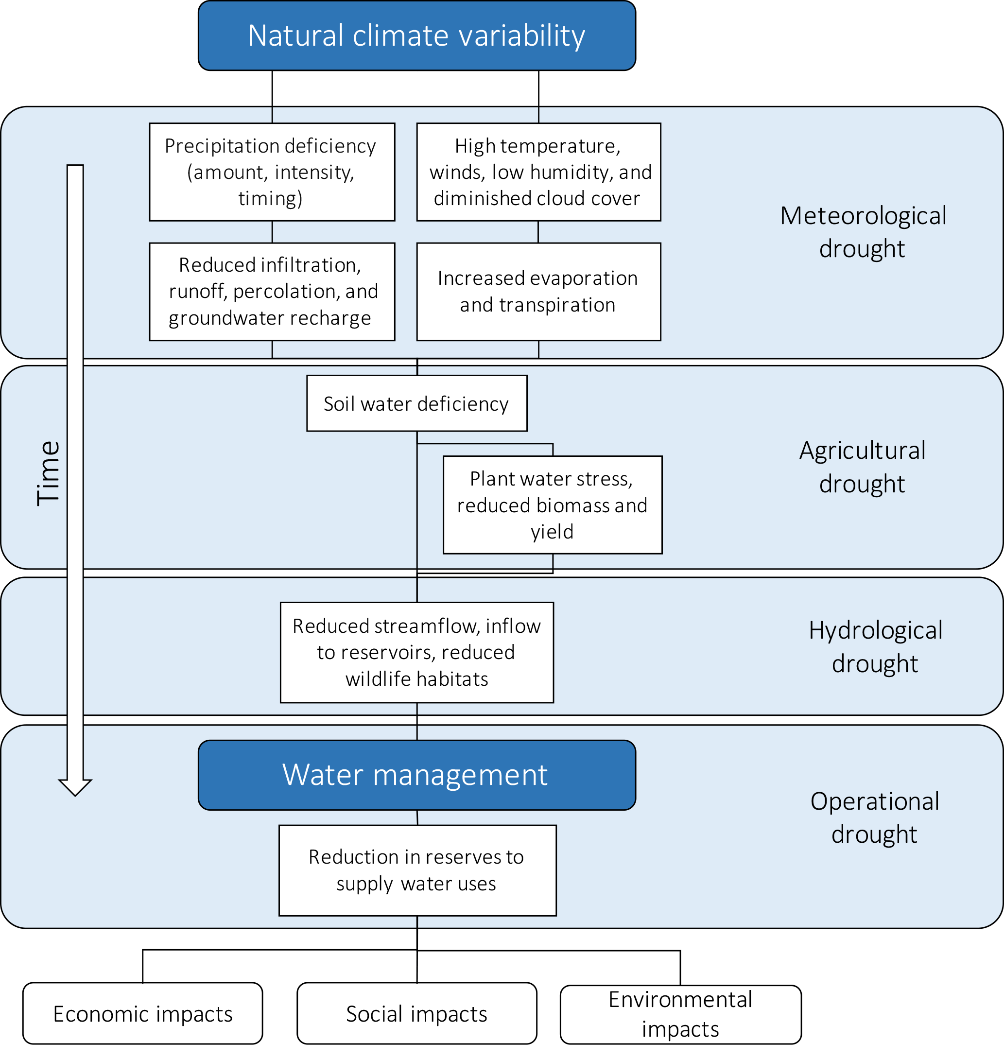
Figure 1Development chain of droughts through time. Meteorological drought, defined as a lack of precipitation over a region for a certain period of time, develops in the short term. Agricultural drought accounts for the plants and crops water stress; it develops in the medium term. Hydrological drought, defined as a period of low streamflow in watercourses as well as lake and groundwater levels below normal, develops in the long term. Operational drought, defined as a period with anomalous supply failures in a developed water exploitation system, develops in the long term. Figure adapted from Spinoni et al. (2016) to include operational drought.
A meteorological drought is defined as a lack of precipitation over a region for a certain period of time (Mishra and Singh, 2010). It develops over the short term (1–3 months) and can extend to longer periods, and is usually associated with the global behavior of the atmospheric circulation (Pedro-Monzonìs et al., 2015). Precipitation is always the core variable to characterize this drought type, with most meteorological drought indexes based on precipitation only (Byun and Wilhite, 1999; McKee et al., 1993). In some cases, especially in regions where droughts can be strongly influenced by evapotranspiration, additional variables such as temperature trends are also considered (Vicente-Serrano et al., 2010; Lorenzo-Lacruz et al., 2010).
Agricultural drought affects, and is defined through, the state of soils and crops in the medium term (3–6 months; Pedro-Monzonìs et al., 2015). This drought type manifests itself with dryness in the root zone and, although rainfall deficiency is a primary cause, precipitation alone is often not enough to describe it. Approaches to characterize agricultural droughts focus on monitoring soil water balance and the subsequent deficit (Palmer, 1965; Narasimhan and Srinivasan, 2005; Hao and AghaKouchak, 2013). The factors involved in this case include vegetation type, soil water holding capacity, wind intensity, evapotranspiration rate, and air humidity (Heim Jr, 2002). In regulated systems, agricultural droughts can usually be restrained with irrigation (Keyantash and Dracup, 2002).
Hydrological drought is defined as a period of exceptionally low flows in watercourses, and lake and groundwater levels below normal (Dracup et al., 1980; Van Loon and Van Lanen, 2012). Related indicators mainly focus on streamflow, as the by-product of every hydro-meteorological process taking place in water catchments (Heim Jr, 2002; Vicente-Serrano and López-Moreno, 2005). More comprehensive indexes can also include snowpack extent, reservoir storage, and groundwater level (Shafer and Dezman, 1982; Keyantash and Dracup, 2004; Staudinger et al., 2014). This drought takes place after a prolonged time of low precipitation and deficient soil moisture and its effects are witnessed in the long-term (6–12 months; Zargar et al., 2011).
These three categories refer to droughts as a natural hazard, i.e., a threat of a naturally occurring event that negatively effects people or the environment (Gustard and Demuth, 2009; Van Loon and Van Lanen, 2013; Laaha et al., 2016). On the other hand, particularly in highly regulated contexts, a dry spell may be caused by natural scarcity of precipitation as well as inconsiderate overuse and/or mismanagement of water resources. Another interesting way to approach drought analysis is, therefore, through the concept of operational (or anthropogenic) drought. Operational drought is defined as a period with anomalous supply failures in a developed water system (Pedro-Monzonìs et al., 2015). It is caused by a combination of two factors: lack of water resources and excess of demand (Mishra and Singh, 2010; AghaKouchak, 2015a). Moreover, it can be further worsened by an inadequate design and management of the water exploitation system and its operating rules (Mishra and Singh, 2010). Operational drought indicators aim at comparing water availability to human water needs and serve as a measure of water well-being, rather than a measure of natural fluctuation as in the case of meteorological, agricultural, and hydrological indicators (Sullivan et al., 2003; Rijsberman, 2006). In the computation of operational drought indicators, the available water is often represented by the streamflow, or a fraction of it, and the water need is usually quantified by a standard per capita or by a fixed nominal demand (Falkenmark et al., 1989; Raskin et al., 1997). Depending on the application scope, operational drought indicators are either river-basin-specific (Garrote et al., 2007; Haro-Monteagudo et al., 2017) or used in studies covering continental or global areas with an annual time resolution (Yang et al., 2003; Oki and Kanae, 2006; Alcamo et al., 2007; Kummu et al., 2010).
When considering a highly regulated water system, i.e., a system where natural water availability is altered by the presence and operation of water infrastructures, traditional drought indicators (e.g., SPI, Standardized Precipitation Index; SPEI, Standardized Precipitation and Evapotranspiration Index; SRI, Standardized Runoff Index) present different shortcomings. On the one hand, meteorological, agricultural, and hydrological indexes often fail at representing drought conditions when regulated lake releases and/or groundwater pumping filter water availability and play a role in magnifying or smoothing drought impacts. Anthropic systems have, in fact, a demonstrated ability to endure meteorological droughts for months, or even years, without suffering consequences, i.e., without incurring a situation of water shortage perceived by the users. An effective planning and management of water resources enables such systems to wisely exploit the combined storage capacities of surface and groundwater reserves and restrain drought (Rijsberman, 2006; Haro et al., 2014a). On the other hand, operational drought indexes are often designed to operate analyses over coarse spatiotemporal resolutions, thus being unsuitable for real-time basin-level drought detection, characterization, and management. Highly regulated systems need ad hoc index formulations tailored to basin characteristics (Wanders et al., 2010; AghaKouchak, 2015b), combining human-controlled variables (e.g., reservoirs and groundwater levels) with uncontrolled hydro-meteorological variables (e.g., precipitation, temperature, natural inflows) to reflect both regulation effects and natural fluctuations in the basin.
A paradigmatic example of a practical and systematic policy for the identification and mitigation of operational droughts is provided by Spain, where public river basin management authorities (Confederaciones Hidrográficas) are bound by law (Ministerio del Medio Ambiente, 2000) to design basin-specific state indexes associated with each main river basin (Ie, Índice de Estado). Most of the basins in Spain are highly regulated and these state indexes are computed as a weighted average of relevant observed variables at selected control points, e.g., precipitation, streamflow, reservoir level, and groundwater level. Each river basin authority has designed its customized formulation for the state index which reflects the hydroclimatic conditions and the water uses of the region (Estrela and Vargas, 2012). The value of the state indexes is monitored monthly and used to trigger water demand and supply measures when entering a drought period, according to the district drought management plan (Garrote et al., 2007; Gómez and Blanco, 2012; Haro et al., 2014a).
Each drought management plan and the relative state index formulation is the result of a long collaborative process including public participation, basin experts, and stakeholders, and provides an effective multi-sector partnership approach for managing drought risk (Carmona et al., 2017). State indexes are the result of a long trial-and-error process mostly begun in the 80s, through which the variable choice and combination have been progressively adjusted to best suit the basin drought management requirements. In the case of the Jucar basin, for instance, the final form of the associated index was established in 2007 with a report by the Confederación Hidrográfica del Júcar (CHJ, 2007a), after 25 years of refinements. This long empirical process produced an index formulation tailored for the Jucar system, which cannot be generalized to different contexts. Similarly, other main Spanish river basins (e.g., the Duero, Ebro, and Guadalquivir river basins) underwent an analogous process and formulated their own state indexes (CHD, 2007; CHE, 2007; CHG, 2007).
Since their establishment in 2007, state indexes have represented the most consistent and extensively applied paradigm of index-based drought management. Thus, Ie constitutes the state of the art for basin-customized operational drought indexes. A reasonable research question is whether the empirical process leading to their design can be formalized, automated, and easily exported to different water systems.
In this study, we contribute the FRamework for Index-based Drought Analysis (FRIDA), which allows for the automatic construction of basin-customized drought indexes for highly regulated water systems. In contrast to traditional empirical approaches, FRIDA uses an advanced feature extraction method that completely automatizes and generalizes the variable selection process for the construction of the index. The selected variables are then combined into a new index that can effectively represent the state of water resources in the basin as well as support the characterization of drought conditions. The feature extraction step is key in FRIDA as it guides the construction of a skillful (highly accurate) and parsimonious (with low input dimensionality) drought index by performing the selection of the best input subset to build a model of a predefined target output representing the drought conditions in the basin.
Specifically, FRIDA is structured in three steps. First, we define a target variable, an appropriately chosen water deficit acting as a proxy for the drought conditions of the considered basin (e.g., water supply deficit, soil moisture deficit), and a dataset of hydro-meteorological variables and traditional drought indicators. Second, we identify Pareto-optimal subsets of variables balancing predictive accuracy and parsimony. In this study, we employed the Wrapper for Quasi-Equally Informative Subset Selection (W-QEISS) to perform this operation (Karakaya et al., 2015; Taormina et al., 2016). Traditional variable selection algorithms are conceived to select only one optimal subset of predictors, while W-QEISS identifies one subset with the highest predictive accuracy, and multiple subsets with similar information content, thus providing more informative results. Moreover, W-QEISS includes two metrics of relevance and redundancy in the search process in addition to the commonly used objectives of accuracy and cardinality, fostering the diversification among the provided solutions (Sharma and Mehrotra, 2014). Third, we choose the preferred predictor subset among the non-dominated solutions based on accuracy, cardinality (i.e., dimensionality), and, possibly, additional factors, including cost and availability of the variable observations. The subset is finally used to calibrate a chosen model class with respect to the target variable, and the drought index is thus completed.
The potential of the proposed framework is demonstrated by the highly regulated Mediterranean basin of the Jucar river, in eastern Spain, where the state-index-based drought management system provides an ideal benchmark for testing the FRIDA index (Andreu et al., 2009; Haro et al., 2014b; Pedro-Monzonís et al., 2014; Macian-Sorribes and Pulido-Velazquez, 2017; Haro-Monteagudo et al., 2017; Carmona et al., 2017). The Jucar state index provides guidelines for the application of FRIDA. First, it facilitates the target variable choice and candidate variable retrieval; second, it allows for the validation of FRIDA predictors selection, and index design steps. FRIDA and state indexes are compared in terms of accuracy in reproducing the drought conditions of the basin, number of variables required for their computation, and general reliability and portability of the methods. The outcome of this analysis consists of demonstrating the validity of a completely automated procedure (i.e., no information on system topology or basin characteristics is required) in recognizing the main drought drivers, and predicting a deficit with accuracy and limited computational effort.
2.1 FRamework for Index-based Drought Analysis
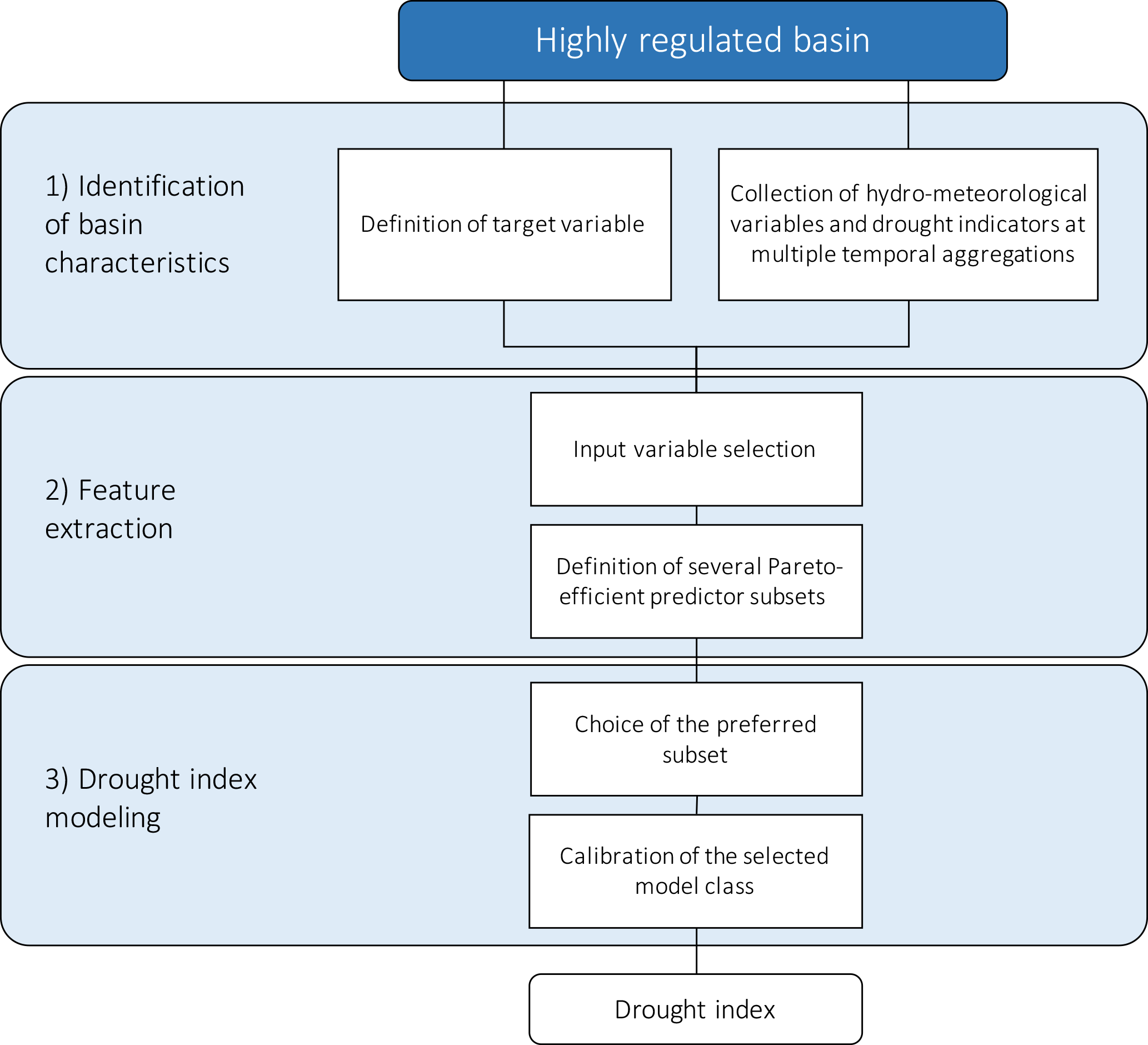
Figure 2FRamework for Index-based Drought Analysis (FRIDA): 1. Identification of basin characteristics, 2. feature extraction, and 3. drought index modeling.
FRIDA designs drought indexes in three steps as reported in Fig. 2.
The identification of basin characteristics is a preliminary empirical process, which consists of the selection of a target variable and the collection of candidate predictors. The target variable is an appropriately chosen water deficit, representative of the actual drought conditions in the basin (e.g., water supply deficit, soil moisture deficit). The dataset of predictors contains the candidate features to reproduce the target variable and consists of observed hydro-meteorological variables and composite drought indicators over different spatiotemporal scales.
Target variable and candidate predictors constitute the input to the “feature extraction” step, the second building block of the framework. This block employs an input variable selection (IVS) algorithm that explores the space of candidate predictors to select Pareto-efficient subsets of predictors with respect to multiple assessment metrics. Most commonly, these metrics quantify the subset accuracy in reproducing the target and the parsimony (i.e., the cardinality of the subset), crucial characteristics for an operational index expected to balance precision and ease of use. In some cases, relevance and redundancy can also be considered in order to explore the input space more effectively. In particular, the metric of relevance favors highly informative subsets (i.e., constituted by predictors that are highly correlated with the target), while the redundancy metric ensures low intra-subset similarity. The objectives of relevance and redundancy are essential to stimulate the search process towards the identification of a diversified and comprehensive set of solutions, which would not be achieved by optimizing cardinality and accuracy only.
In this work, we use an advanced IVS algorithm called the Wrapper for Quasi-Equally Informative Subset Selection. W-QEISS provides as output a number of efficient subsets that are collected in a selection matrix.
In the “drought index” modeling block, the preferred efficient solution is selected by the user, balancing the trade-off between competing objectives and, possibly, considering additional operative needs neglected in the IVS search (e.g., cost and reliability of the variable monitoring). Lastly, an appropriate regressor is fit to the sample dataset of Pareto-efficient inputs and the target variable. The choice of model class is determined by the application of interest. In general, highly non-linear learning machines like artificial neural networks (ANNs) provide a good balance between accuracy and flexibility. On the other hand, such black-box models lack intuitive interpretability and might be unsuitable for applications that affect several stakeholders and require a wide acceptance of the tool to be employed (Estrela and Vargas, 2012). In these cases, a simpler model (e.g., a linear model) might be preferred, as it grants an immediate understanding of the physical meaning, though at the price of poorer approximation skills.
2.2 Feature extraction via the Wrapper for Quasi-Equally Informative Subset Selection
Feature extraction techniques, employed in the second block of FRIDA, are an ensemble of data pre-processing algorithms that transform the original input dataset into a more compact, while still highly informative, subset (Cunningham, 2008). Among the feature extraction algorithms, IVS techniques specifically address the problem of the reduction of the input space by identifying the relevant predictors to be used to calibrate a model of the target variable (Bowden et al., 2005). There are two main classes of IVS techniques: “filters” and “wrappers”. Filters evaluate the relevance of each variable separately, computing an error metric on the features (Yang and Pedersen, 1997; Sharma, 2000; Galelli and Castelletti, 2013). Wrappers, on the other hand, assess the relevance of a variables ensemble, evaluating the prediction performance of a given learning machine calibrated on the input set, and thus considering the interactions and dependencies between variables (Guyon, 2003). In terms of performance, wrappers are often more accurate than filters, although computationally more intensive (Galelli et al., 2014).
In this study, we used W-QEISS as a wrapper (Karakaya et al., 2015; Taormina et al., 2016). The W-QEISS algorithm receives as input the set X of candidate predictors, i.e., and the trajectory y of the target variable. The algorithm is composed of three main steps (Karakaya et al., 2015), as illustrated in Fig. 3.
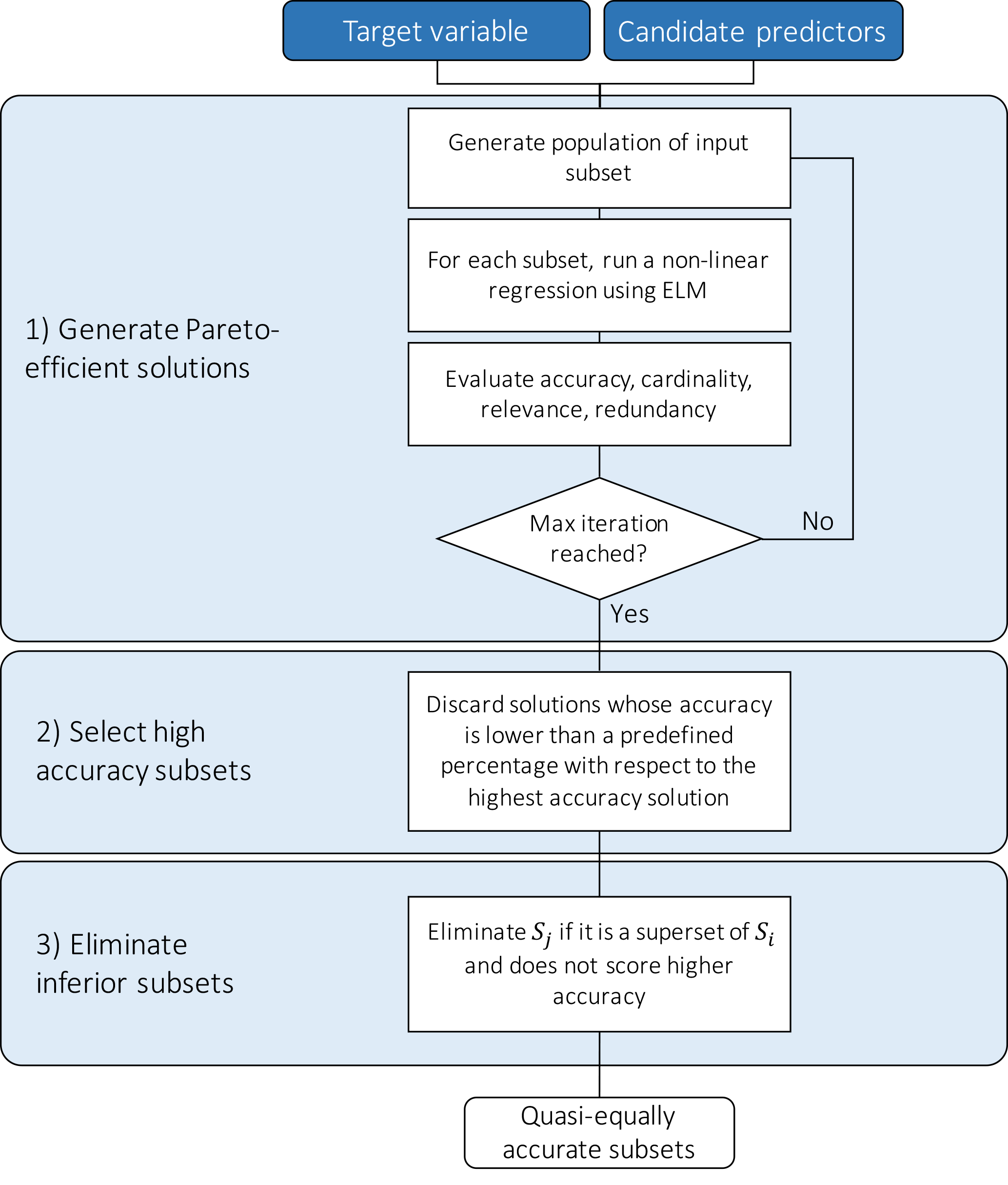
Figure 3The W-QEISS flowchart. Step 1: generate Pareto-efficient solutions with respect to the four objectives of relevance, redundancy, cardinality, and accuracy; step 2: select high accuracy subsets; step 3: eliminate inferior subsets.
-
Step 1: a set A⊆X of Pareto-efficient solutions is built according to the four-objective functions of relevance f1(⋅), redundancy f2(⋅), cardinality f3(⋅), and accuracy f4(⋅). A global multi-objective optimization algorithm is employed to explore the space of possible subsets. In this study, we use the self-adaptive Borg Multi-Objective Evolutionary Algorithm (MOEA; Hadka and Reed, 2013), which has shown to outperform other benchmark evolutionary algorithms in terms of number of solutions returned, ability to handle many-objective problems, ease of use, and overall consistency across a suite of challenging multi-objective problems (Reed et al., 2013). A learning machine is used to compute the predictive accuracy f4 of each set. In this study, we employ extreme learning machines (ELMs; Huang et al., 2006), belonging to the family of ANNs, which were shown to provide a good performance in terms of accuracy and flexibility in a variety of problems, while being up to a thousand times faster than benchmark feedforward ANNs (Huang et al., 2012). ELMs, in fact, bypass the time consuming gradient-based search of optimal neuron parameters required by traditional ANN techniques, by defining randomly parameterized hidden nodes, and subsequently optimizing their output weights. Such optimization is solved through a one-step matrix product and essentially amounts to learning a linear model.
However, we do not expect the choice of the learning machine or MOEA to be crucial for the attainment of the result. A different benchmark MOEA (e.g., NGSAII, MOEAD, eps-MOEA) is likely to achieve a comparable result, although requiring a possibly significant effort in the manual calibration of the evolution parameters, which is automated in Borg MOEA. Similarly, ELM could in principle be substituted by other ANN techniques, although incrementing the computational time to possibly unbearable levels, given the multiple calibration and validation processes reiterated in W-QEISS.
-
Step 2: among the Pareto-efficient subsets, the maximum value of accuracy is identified, associated with subset . Then, solutions with significantly lower accuracy are discarded from ensemble A, obtaining Aδ. The ensemble Aδ contains quasi-equally informative subsets with respect to , i.e., subsets that have (almost) the same predictive accuracy with respect to a given model class. When the dataset of candidate variables presents a significant correlation among features, numerous subsets characterized by a wide range of cardinalities are generally available to achieve a relative small range of accuracies. This is often the case in environmental problems, where spatial and temporal correlation of hydro-meteorological variables and associated indicators is significant. Therefore, at this stage, the accuracy metric is used to retain accurate solutions only, provided that they feature different cardinalities and predictor combinations.
Formally, on the basis of a predefined small value of δ, Si is δ-quasi-equally informative to subset if
-
Step 3: the final ensemble is computed after the elimination of the inferior subsets. The subset Sj is considered inferior to Si, if it is a superset of Si, and does not score higher accuracy. Formally
Si⊂Sj and f4(Si)≥f4(Sj).
In this step, all subsets contained in Aδ are compared in order to find possible inferior subsets and eliminate them. By doing this, the final ensemble of δ-quasi-equally informative subsets is provided as output of the procedure and reported in a selection matrix.
The W-QEISS algorithm differs from a traditional IVS approach as it introduces the consideration that, for a given cardinality, multiple subsets of variables can have almost indistinguishable accuracy performance. The outcome of W-QEISS variable selection is thus not a single most accurate subset for each cardinality, but a pool of δ-quasi-equally accurate solutions among which the preference can be determined by other metrics not directly considered in the optimization (e.g., cost and reliability of the variable observation).
Another innovative feature of the W-QEISS approach relies on the formulation of a four-objective optimization problem. Besides the two traditional objectives of accuracy ad complexity commonly employed in wrappers, W-QEISS includes two other metrics of relevance and redundancy (Sharma and Mehrotra, 2014). The maximization of accuracy ensures a precise reproduction of the data, while the minimization of cardinality aims at simplifying the final models. These characteristics are key for an operational index, expected to balance precision and ease of use. Relevance and redundancy optimization is instead an asset for an effective subset search process, as it fosters the diversification of the solutions explored within the MOEA algorithm, guaranteeing low intra-subset similarity and high information content of the solutions. A two-objective search based on cardinality and accuracy would only, in fact, identify optimal solutions, but at the same time disregard a number of quasi-equally informative subsets with an almost identical operational behavior. The identification of such alternative solutions, nevertheless, grants flexibility and a multiplicity of options for the expert-based choice of the preferred subset, where certain combinations of predictors can be favored according to case-specific operative purposes, e.g., more robust or less costly data gathering process, enhanced acceptability, or immediacy of the index.
Three of the four objectives formulations make use of the symmetric uncertainty (SU), a measure of the dependence and similarity between two variables (Witten and Frank, 2005). SU assumes values between 0 (independent variables) and 1 (complete dependence) and is computed for two features A and B as
where H(⋅) is the entropy of variable (⋅) (see for instance Scott, 2012 for the definition).
W-QEISS bases its objectives formulation on information theory, as discussed in Karakaya et al. (2015). Information theoretic criteria (e.g., SU, mutual information, and partial mutual information) do not assume any functional relationship between the variables and thus are well suited to quantify the dependence between two variables in any modeling context (MacKay, 2003). Other objectives formulations could in principle be explored, for instance substituting the use of symmetric uncertainty with more traditional correlation coefficients, although with the risk of losing generality by assuming linear dependence between variables.
The four assessment metrics are formulated as follows:
-
Relevance f1(S): to be maximized, is formulated as
where the term SU(xi,y) represents the symmetric uncertainty between the feature xi and the output y. The relevance is therefore a measure of the explanatory power of the features with respect to the output.
-
Redundancy f2(S): to be minimized, is formulated as
where SU(xi,xj) represents the SU between two features xi and xj. High redundancy thus means high similarity between the features. By minimizing the redundancy, the algorithm ensures that the search will be oriented towards the selection of subsets with mutually dissimilar features.
-
Cardinality f3(S): to be minimized, is formulated as
where |S| is the number of predictors within the subset. Its minimization guarantees that the resulting model will not be unnecessarily complex.
-
Accuracy f4(S): to be maximized, is formulated as
where SU is the correlation, measured in SU, between the observed output y and the prediction obtained from the model.
The Jucar river basin occupies an area of 42 989 km2 located in the eastern part of Spain (see Fig. 4). The territory is mainly mountainous in the interior part, while the center-eastern section shows a vast plain system ending into the Mediterranean Sea. The territory is characterized by various climatic conditions of which sub-humid and semi-arid are largely dominant. The main rivers of the area are the Jucar, Mijares, and Turia, covering altogether more than 80 % of the total mean areal flow. The subterranean runoff is very relevant, providing 74 % of the contribution to the river network (CHJ, 2007a).
Since the mean value of the total annual runoff (1747 Mm3 from 1940 to 2009) almost equals the annual water demand (1640 Mm3), water scarcity and droughts have long been perceived as primary issues for agricultural, social, economic, and environmental reasons. On the other hand, meteorological droughts in the Jucar basin can be endured for several years without suffering any consequences, due to the highly regulated water system set in the area. There are three main large surface reservoirs in the region: Alarcón, Contreras, and Tous (maximum capacity: 1118, 444, and 378.6 Mm3, respectively). In addition, most aquifers in the basin are intensively exploited to support agricultural supply and are currently experiencing a significant depletion due to over-drafting, which, in turn, affects the river flows.
In such a highly regulated basin with long overyear storage, water scarcity is not a necessary condition derived from a meteorological drought (CHJ, 2007a; Carmona et al., 2017). Thus, traditional drought indexes fail at detecting the timing and severity of the incidence of a drought, and an ad hoc monitoring system was conceived to properly capture the hydrological status of the catchment. The monitoring system is based on the formulation of a basin-specific index, namely the state index (Ie, Índice de Estado). The state index was constructed empirically by the Jucar river basin authority (CHJ), with the intent of highly correlating with the water scarcity conditions in the basin, in order to support drought management and the implementation of the actions considered in the drought management plan (CHJ, 2007a). For those purposes, the index is developed after identifying the water sources for every main demand in the basin and the selection of representative variables to characterize the status of those sources.
The total state index Ie is computed as a weighted mean of 12 partial Ie. Partial Ie are obtained by normalizing hydro-meteorological indicators (Vi) belonging to the following categories (see Fig. 4):
-
The mean monthly storage of one or more reservoirs combined (Mm3; 2 storage indicators);
-
The mean streamflow contribution of the last 3 months (Mm3; 4 flow indicators);
-
The mean monthly piezometric level (m; 3 piezometer indicators);
-
The areal precipitation of the last 12 months (mm), computed by averaging the values observed by multiple pluviometers (3 precipitation indicators).

Figure 4Map of the Jucar river basin network. The colored markers represent the variables considered for the state index calculation. S: reservoir storage, F: streamflow, Pz: piezometer, Pl: pluviometer. Streamflow and piezometers markers are located in correspondence to the relative measurement station, while storage and pluviometer markers are put in the center of the polygon formed by connecting the multiple measurement points used for their computation.
Each “indicator” (Vi) is consequently normalized to obtain 12 partial Ie values:
where Vm, Vmax, and Vmin are the mean, maximum, and minimum values of each indicator time series, respectively. The storage and precipitation monthly time series are normalized with respect to maximum and minimum values of the considered month, while piezometers and river flows are normalized with respect to the complete historical time series. The partial Ie result as normalized indexes between 0 and 1, where Ie>0.5 indicate a higher than average value of Vi. Once the partial Ie have been computed, they are aggregated as a weighted sum to obtain the total Ie. The weights are established according to the demand class associated with the indicator, ranging from class A (demand > 100 hm3 year−1) to D (demand < 10 hm3 year−1).
The Jucar river basin represents a Mediterranean drought-prone and highly regulated basin, featuring one of the most innovative and effective drought management systems, relying on the formulation of an empirically constructed basin-specific drought index (Andreu et al., 2009; Haro et al., 2014b; Haro-Monteagudo et al., 2017; Carmona et al., 2017). As a consequence, it represents the state of the art for basin-customized operational drought indexes employed for drought-restraining purposes, and a remarkable benchmark to test and validate the proposed FRIDA methodology.
For the presentation of the numerical results we follow the workflow proposed in Fig. 2 . The length of the dataset available for the experiments is N=174 data points, corresponding to monthly values in the period 1986–2000, and nx=28 is the number of candidate predictors used (Zaniolo et al., 2018). The parameterization of W-QEISS was adjusted using available guidelines given by Huang et al. (2006), Karakaya et al. (2015), and a trial-and-error process. For Borg MOEA, we set the number of function evaluation equal to 2 million, while the number of hidden neurons in the ELM, presenting a sigmoidal activation function, was set to 30. A k-fold cross-validation process (with k=10) was repeated 5 times and the average resulting value was used to estimate the predictive accuracy of each model. The W-QEISS experiment with such settings was run 20 times to filter out the random component of the process, and the results presented below are obtained by merging the Pareto fronts obtained by each repetition into a final Pareto front of non-dominated solutions.
4.1 Identification of the basin's characteristics
In the first report concerning the Ie development (CHJ, 2007b), the index was validated for the time span from January 1986 to June 2000 against the supply deficit recorded in the basin with respect to agricultural and urban water demand, and the procedure for the state index computation was approved. To ensure comparability between the Ie and the FRIDA constructed index, we decided to employ the same supply deficit as target variable for the application of the FRIDA approach to the Jucar case study. The Jucar supply deficit employed in this work was simulated via the AQUATOOL model (Andreu et al., 1996). The model can run in simulation mode with a monthly time step, and it is conceived in the form of a flow network with oriented connections reproducing water losses, hydraulic relations between nodes, reservoirs and aquifers, and flow limitations based on elevation. Within AQUATOOL, complex processes such as evaporation and infiltration are effectively reproduced. The modeled supply deficit, employed as target variable, represents the monthly nominal shortage of water conveyed to the irrigation districts, and is only quantifiable a posteriori, when the water shortage has already jeopardized the fields. On the other hand, a drought index can be constantly monitored, and thus represents a valuable management tool for restraining drought impacts and identifying effective drought management strategies.
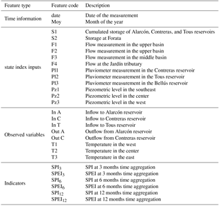
The database of candidate input variables was assembled by retrieving the available observed variables in the basin and computing traditional drought indicators at multiple time aggregations. The resulting candidate predictors, listed in Table 1, are the following:
-
two temporal features: date of the measurement and month of the year (Moy);
-
12 monthly observed variables, current inputs to the Ie, reported in Fig. 4: average monthly storage and groundwater levels, average 3-month river runoff, and cumulated areal precipitation over 12 months;
-
eight additional observed variables in the basin: outflows from, and inflows to, the main reservoirs, and mean monthly areal temperatures;
-
six traditional drought indicators: the Standardized Precipitation Index (SPI) and the Standardized Precipitation and Evapotranspiration Index (SPEI). SPI and SPEI indicators are computed on mean monthly data over the entire basin for 3-, 6-, and 12-month time aggregations. SPI requires as input the precipitation and SPEI requires precipitation and temperature, as it uses the difference between precipitation and potential evapotranspiration as reference variable.
Their values express the water availability conditions of a basin in terms of units of standard deviation from the mean: negative (positive) values indicate drier (wetter) conditions than average (see McKee et al., 1993; Vicente-Serrano et al., 2010 for details on definition and calculation of these indicators).
Table 1Set of candidate input features for the feature extraction step via W-QEISS.
4.2 Feature extraction via W-QEISS
The result of the W-QEISS algorithm is not a single most-accurate set of variables for a given cardinality, but several quasi-equally informative subsets, whose accuracy is lower than the best one by a small percentage (δ⋅100 %). Figure 5 represents a “selection matrix”, which reports the composition of each alternative subset of predictors within 15 % of accuracy with respect to the highest one. The value δ=0.15 was chosen since it provides a reasonable trade-off between the number of solutions and their accuracy. The accuracy is measured in symmetric uncertainty between the target variable and the ELM calibrated using the reported subset.
The alternative subsets are sorted in ascending order of cardinality (from top to bottom), and accuracy (within each cardinality level). A rectangular marker is placed at the intersection between the row identifying a given subset and the columns corresponding to the selected predictors. The marker color varies with the cardinality of the subset, with lighter shades of gray indicating smaller subsets. In this case the cardinality spans from 3 to 9 features. The highest accuracy is reported in red and recorded for subset number 14. The five corresponding selected predictors, marked on the horizontal axis with a blue background, are the following:
-
Moy: month of the year;
-
S1: total storage aggregated for the reservoirs Alarcón, Contreras, and Tous;
-
F3: river flow measured in the Jucar middle basin, after the confluence with smaller rivers Jardín and Lezuza coming from the southwest;
-
Pz2: groundwater level measured at the piezometer situated in the central area of the basin, in correspondence with a rainfed agricultural area;
-
SPEI6: SPEI at 6 months time aggregation computed with precipitation and temperature data averaged for the whole basin.
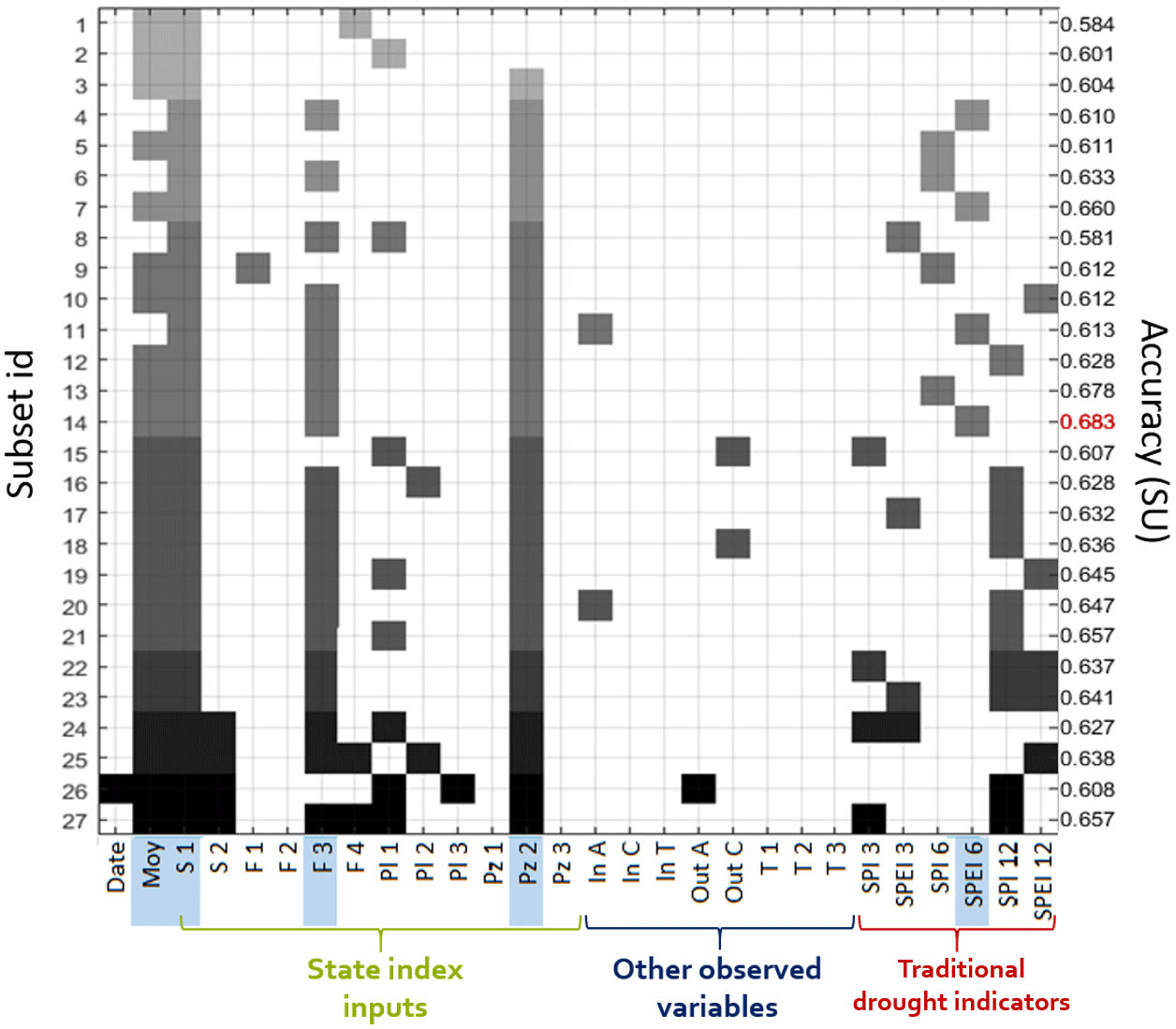
Figure 5Selection matrix: the left vertical axis represents the subset number (id) and the right vertical axis the corresponding accuracy measured in SU. A colored marker is put in correspondence with the variables, listed on the horizontal axis, selected by each subset. The shade of gray is an indication of the cardinality of the subset, lighter shades for lower cardinality. The highest accuracy is reported in red and the corresponding variables, constituting the most accurate subset, have a blue background.
From the analysis of the selection matrix, several insights can be gained from modeling and decision-making viewpoints. To begin with, insights into the relevance of a predictor can be obtained from the detection of the vertical bars traced by joining markers across multiple rows. Uninterrupted bars indicate strongly relevant predictors that cannot be substituted by other input combinations without incurring a substantial drop of predictive accuracy. This is the case for the cumulated storage of the three main reservoirs Alarcón, Contreras, and Tous (S1). This information is essential to the final model, as the exclusion of such predictors highly affects the model performance.
Increasing gaps in the vertical bars are found when considering predictors with progressively weaker relevance, while irrelevant inputs are recognizable by isolated markers or their total absence. The variables Moy, F3, and Pz2 are considered relevant variables, as they are selected quite frequently, although high accuracy solutions exist that do not make use of all of them. Finally, the variable SPEI6, while included in the most accurate subset, is overall present in four subsets only, whereas in other solutions with comparable accuracy it is replaced by different predictors, mainly carrying a similar precipitation-based information, such as pluviometer measures, or SPI/SPEI indicators at different time aggregations.
The presence of alternative subsets helps explore the trade-off between multiple measures of predictive accuracy with respect to other metrics not directly considered in the optimization routine, and the choice of the preferred subset is determined by the index application. Given the cardinality, one can decide to sacrifice a small amount of predictive accuracy for an easier-to-yield (or more reliable) combination of predictors. For example, with a loss smaller than 1 % in accuracy, subset 13 selects SPI6 instead of SPEI6. This possible replacement is interesting from an operational point of view as SPI is easier to compute than SPEI. In fact, SPI only requires the precipitation for its computation whereas precipitation and temperature or evapotranspiration are needed for the computation of SPEI. In addition, even after the preferred subset is chosen and the system is operating, knowing that one specific predictor can be replaced by another (or multiple) predictor(s) can aid management in case of monitoring network maintenance or instrument failure. When the main predictor is not observable, one can temporarily resort to alternative predictors incurring a minimum loss of accuracy.
An additional consideration is related to the possibility to effectively address the uncertainty deriving from the choice of model inputs (Taormina et al., 2016). When multiple alternative subsets are provided, it is possible to explore the uncertainty related to the selection of predictors yielding similar accuracy. For instance, in this case study, we can observe that almost all subsets carry groundwater and rain information, but while the piezometric level is consistently provided by Pz2, the source of the precipitation information highly varies among the precipitation-based features (pluviometers or other SPI/SPEI indicators).
Finally, through the selection matrix analysis we can compare the features selected by W-QEISS and the variables that constitute the state index input set. Apart from sporadic single selections, all the observed variables not included in the state index are consistently discarded by the W-QEISS as well, suggesting that the algorithm comes to the same conclusion as the Spanish experts considering inflows, outflows, and temperatures as non-relevant for the description of the state of water resources in the Jucar river basin. Note that this result is a consequence of the use of the nominal agricultural demand to compute the target deficit. Temperature information is likely to become relevant if a real, weather-influenced, agricultural demand is employed instead. The feature month of the year is not explicitly an input to the state index, nevertheless, analogous information is implicitly included in the Ie through the normalization of the indicators described in Eq. (7). On the other hand, several features are considered in the Ie, but generally neglected by the W-QEISS selection. Among them, two out of three piezometers, the river flows upstream from the reservoirs, one pluviometer and the storage at Forata. These inputs are probably redundant due to their spatial correlation. Spatial variability is considered in the computation of Ie by including several spatially distributed observations of the main information categories: two measures of reservoir storages, four of river flows, three groundwater levels, and three precipitation measures. Conversely, the selection matrix supports the gain of a deeper understanding of the spatial interdependence of variables by identifying the best location for measuring the variables, sparing the need for several distributed measures. The highest accuracy-subset, in fact, selects only one variable out of each category: one storage, one river flows measure, one piezometer, and a spatially distributed precipitation information, i.e., SPEI6 which replaces three areal pluviometers.
4.3 Drought index modeling
Among the pool of solutions, the choice of the preferred subsets is driven by the index application. For instance, an online use of the index that requires its frequent computation may benefit from an agile, easy-to-observe subset. With respect to the highest accuracy solution (subset 14), for instance, subset number 7 neglects predictor F3 thus presenting lower cardinality with an accuracy loss of only 3 %. Similarly, the already mentioned subset 13 contains an easier-to-compute indicator (SPI instead of SPEI) with a negligible performance degradation. Nevertheless, for our methodological purpose we will employ the most accurate subset 14, as we are interested in discussing the potential of the method.
Concerning the model class choice, a highly flexible non-linear model is likely to yield the highest accuracy in reproducing the target. However, strong non-linearity and black-box behavior typically result in poor interpretability, a feature that is detrimental to the use of the index for management purposes as in the Jucar system, where restrictive measures in water use are activated when certain threshold values of the state index are reached. As a consequence, the index outcome exerts a direct influence on many water-related activities requiring an easily interpretable and widely acceptable tool.
The calibration of a linear model on the chosen 5-dimensional subset seems to be a good compromise between accuracy and transparency. As mentioned above, the feature Moy represents the succession of the months in the year, and is an expression of the seasonality of hydro-meteorological processes. Moy is constructed as the repetition of an array of numbers from 1 to 12 for the length of the considered time horizon, and thus presents a discontinuous shape: a slow and steady increase followed by a steep decrease in correspondence to the onset of a new year. While the non-linear models employed in the feature selection can effortlessly handle such an intermittent vector, linear models struggle with similar shapes. We therefore decided to account for the seasonality in the linear model indirectly, i.e., excluding Moy from the predictors set, but, consistently, considering seasonality by subtracting the annual cyclo-stationary mean from the predictors time series.
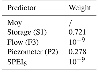
The calibrated linear model representing the supply deficit is reported in Fig. 6 and provides a very satisfying result, with an accuracy measured with the coefficient of determination in cross validation of , significantly higher than the scored by the state index, and a set of weights of immediate physical interpretability reported in Table 2. By inspecting the weights, one can notice that those assigned to the predictors “flow” and SPEI6 are very low, although not null, and the index trajectory is mainly determined by the “storage” and “piezometer” values. S1 and Pz2, in fact, describe the trajectories of the main water reservoirs of the region, lakes and groundwater, whose fluctuations are the result of natural variability as well as human regulation, mainly for irrigation purposes.
Table 2Weights of the linear model calibrated for the optimal subset of predictors. The predictor Moy (month of the year), providing seasonal information, is not directly included in the weights optimization but it is accounted for by subtracting the annual cyclo-stationary mean from the predictors time series.
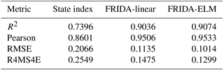
As a further analysis, we reiterated the model calibration and cross-validation steps with a more complex, highly flexible model class, the ELM architecture, which scored an accuracy of . On the one hand, the arguably insignificant 0.005 % improvement in accuracy of ELM with respect to the linear class probably does not justify the loss of immediacy and transparency induced by the transition to a black-box model. On the other hand, this experiment proves the robustness of the linear model in constituting the model class of choice for this drought index. In Table 3 we report a more detailed comparison between state index, FRIDA-linear and FRIDA-ELM indexes with several accuracy metrics. The analysis of other metrics seem to reinforce the conclusions drawn by considering R2 only: both FRIDA indexes (linear and ELM) outperform the state index quite significantly, while the difference among them is negligible, although the non-linear index is always the top performing.
Table 3Accuracy of the state index, FRIDA-linear, and FRIDA-ELM in reproducing the supply deficit, quantified in terms of coefficient of determination R2, the Pearson correlation coefficient, the root mean square error (RMSE), and the fourth grade root mean square error (R4MS4E).
The reported metrics do not distinguish between errors above and below the target deficit. Indeed, we consider these two error types to be of comparable importance. On the one hand, the underestimation of a deficit value may find the water users unprepared to face a serious drought. On the other hand, the overestimation of drought conditions may ignite repeated false alarms that will compromise the index trustworthiness and its efficacy in triggering an alert state. Therefore, rather than penalizing an error above or below the target trajectory, we find it more compelling to focus on errors in the most crucial drought situations i.e., at the maximum level of deficit recorded. One way of doing so is considering R4MS4E, as in Table 3, which penalizes errors in the deficit peaks. Another specific assessment tool for analyzing the indexes performance during critical droughts is the confusion matrix, reporting the classification performance of critical droughts, here arbitrarily defined as months reporting deficit values above the 85th percentile (Tables 4, 5, 6). The rows of the confusion matrix represent the instances in a predicted class, while the columns represent the instances in an actual class. Consequently, the main diagonal reports the number of correctly classified points. Cells outside the main diagonal specify the errors: the value in the bottom-left cell (first column, second row) indicates a situation in which the index does not recognize an ongoing drought, while the value in the top-right cell (first row and second column) indicates the number of false alarms. The FRIDA-ELM confusion matrix seems to significantly exceed the competitors performances by having an error of only 0.57 % of the times, as opposed to the 10.91 % of Ie, and the 6.3 % of FRIDA-linear.
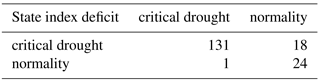
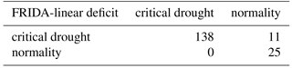
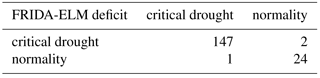
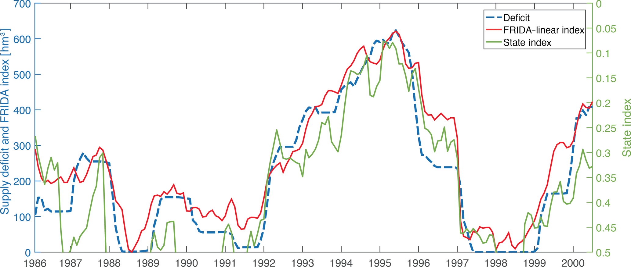
Figure 6Comparison between the FRIDA-linear index (red plot, blue scale on the left) and the state index (green plot, green scale on the right) in reproducing the monthly aggregated supply deficit (blue dashed plot, blue scale on the left). The FRIDA index presents a higher similarity with the deficit and only requires 5 inputs instead of the 12 required by the state index.
The purpose of this study is to contribute to the identification of drought management strategies able to improve the efficiency and resilience of drought-prone regulated water systems. This problem is considered urgent as the analysis of climate trends shows that drought frequency and severity are intensifying all over Europe, particularly in the Mediterranean area.
This work explores the potential of drought indexes as a management tool for the purpose of containing drought impacts. Since traditional indicators are often inadequate to characterize water availability conditions in highly regulated contexts, a novel framework for the construction of customized basin-specific drought indexes is proposed. This framework relies on the employment of a feature extraction technique, the Wrapper for Quasi-Equally Informative Subset Selection (W-QEISS). Given a set of information collected in the basin, W-QEISS features a deep learning machine that automatically selects the most suitable input set for the construction of a model reproducing the target variable, i.e., a ground truth representative for the state of water resources in the basin. Specifically, W-QEISS performs the search process in a four-dimensional metric space of predictive accuracy, cardinality, relevance, and redundancy. On top of that, the W-QEISS algorithm is designed to identify one subset with the highest predictive accuracy and multiple subsets with similar information content (i.e., quasi-equally informative subsets). This provides insights on the relative relevance of the variables and a deeper understanding of the underlying physical processes taking place in the basin. The choice of the preferred input set and model class balance accuracy and practicality of the index. The efficacy of the FRIDA methodology is strongly dependent on data availability, in terms of predictors diversity and numerosity, and length of the time series. FRIDA is best applicable in contexts where an extensive monitoring system has been in place for long enough to allow a consistent and informative dataset for the index calibration. However, while some hydro-meteorological variables are easy to monitor and most often available (e.g., precipitation, temperature), the accessibility of soil moisture, groundwater table level, snowpack extent, air humidity etc., may represent a problem. When a key drought-driving variable for the context at hand is absent from the input set, the efficacy of FRIDA is undermined.
The application of FRIDA in the Jucar river basin case study has successfully demonstrated the suitability of the framework to design a basin-specific drought index. Firstly, the automatic variable selection yields an immediate and informative result, which presents strong similarities with the empirical expert-based variable set employed by the CHJ, while involving a significantly lower number of features (5 variables instead of the 12 required by the state index). Secondly, the newly computed FRIDA-linear index outperforms the official Spanish state index in terms of accuracy in reproducing the target variable, while maintaining immediate interpretability.
However, one of the reasons why the Ie enjoyed such wide acceptance among the Jucar stakeholders is related to the widely comprehensive approach employed for its construction. All water users, in fact, feel represented in the index through at least one variable being observed in the proximity of their water-related activity, even if such a variable is low-weighted or redundant when computing the basin-wide aggregated indicator. The FRIDA approach does not ensure such a representation of all water users, although it appears as a more rigorous and efficient alternative to the inclusive CHJ approach. Moreover, FRIDA is a portable methodology, suitable for the many drought-prone contexts in need of a drought management plan. In conclusion, the aim of arranging an effective framework for the construction of basin-customized combined drought indexes can be considered achieved. The indexes constructed with FRIDA have proven to be an asset for (i) representing drought conditions in highly regulated basins, where traditional indexes tend to fail; (ii) gaining a deeper understanding of the hydro-meteorological processes taking place in the basin; and (iii) constituting a valid alternative to the Spanish approach for the state index design, thus supporting appropriate drought management strategies, such as triggering drought-restraining response measures.
The already valid results achieved by this study open new possibilities for the use of basin-specific drought indexes. Further research efforts could be addressed for exploring the potential of employing FRIDA indexes in directly informing water management operations. Additionally, the possibility of forecasting such indexes can be tested in order to timely prepare for upcoming dry seasons. We expect that the projection of a drought index fosters the adoption of a proactive (as opposed to the current reactive) approach in facing a drought. Proactivity promotes a shift from costly and often belated mitigation measures to preventive actions that will grant flexibility to timely prepare for upcoming droughts, while reducing costs associated with drought impacts and restrictions.
Ultimately, FRIDA can represent an asset for improving the system resilience under a changing climate. Despite the fact that FRIDA is conditioned with historical data, one can imagine that in the short term, the interactions and relative role of drivers in causing a drought hold unchanged. In this case, the index formulation remains valid in the context of a changing climate. In the long term, nevertheless, this hypothesis may cease to hold, we thus suggest a frequent reiteration of the FRIDA procedure to monitor the evolution of drivers and dynamics leading to a drought in the basin. For example, in a groundwater-dominated system as the Jucar basin, the piezometer information is likely to remain essential in a future climate, but, at the same time, we can expect evapotranspiration processes to increase their drought-propelling role, as climate change induces a general increase in temperatures. In other contexts, e.g., snow-dominated catchments, the role of snow may lose priority due to a diminishing winter snowpack reserve. FRIDA will thus represent a valuable tool to support the analysis of the dynamic role of drivers in drought evolution under a changing climate.
The complete open source dataset employed for the feature selection step can be downloaded from http://doi.org/10.5281/zenodo.1185084 (Zaniolo et al., 2018). A detailed description of FRIDA, including both data and codes, is available at http://www.nrm.deib.polimi.it/?page_id=2438.
The authors declare that they have no conflict of interest.
The work has been partially funded by the European Commission under the
IMPREX project belonging to Horizon 2020 framework programme (grant no.
641811). The authors would like to thank the planning office of the
Confederación Hidrográfica del Júcar (CHJ) for providing
the data used in this study.
Edited by: Elena
Toth
Reviewed by: two anonymous referees
AghaKouchak, A.: Recognize anthropogenic drought, Nature, 524, p. 409, 2015a. a
AghaKouchak, A.: A multivariate approach for persistence-based drought prediction: Application to the 2010–2011 East Africa drought, J. Hydrol., 526, 127–135, 2015b. a
Alcamo, J., Flörke, M., and Märker, M.: Future long-term changes in global water resources driven by socio-economic and climatic changes, Hydrolog. Sci. J., 52, 247–275, 2007. a
Andreu, J., Capilla, J., and Sanchís, E.: AQUATOOL, a generalized decision-support system for water-resources planning and operational management, J. Hydrol., 177, 269–291, 1996. a
Andreu, J., Ferrer-Polo, J., Pérez, M., and Solera, A.: Decision support system for drought planning and management in the Jucar river basin, Spain, in: 18th World IMACS/MODSIM Congress, Cairns, Australia, vol. 1317, 2009. a, b
Bowden, G. J., Dandy, G. C., and Maier, H. R.: Input determination for neural network models in water resources applications. Part 1 – Background and methodology, J. Hydrol., 301, 75–92, https://doi.org/10.1016/j.jhydrol.2004.06.021, 2005. a
Byun, H.-R. and Wilhite, D. A.: Objective quantification of drought severity and duration, J. Climate, 12, 2747–2756, 1999. a
Carmona, M., Máñez Costa, M., Andreu, J., Pulido-Velazquez, M., Haro-Monteagudo, D., Lopez-Nicolas, A., and Cremades, R.: Assessing the effectiveness of Multi-Sector Partnerships to manage droughts: The case of the Jucar river basin, Earth's Future, 5, 750–770, https://doi.org/10.1002/2017EF000545, 2017. a, b, c, d
Changnon, S. A.: Detecting drought conditions in Illinois, Circular (Illinois State Water Survey), 1–36, Illinois, USA, 1987. a
CHD: Plan Especial de Actuación en situaciones de alerta y eventual sequía, Plan Especial de Actuación en situaciones de alerta y eventual sequía en la cuenca del Duero, TYPSA, Valladolid, 2007. a
CHE: Plan especial de actuación en situaciones de alerta y eventual sequia en la cuenca hidrográfica del Ebro, MARM, Zaragoza, 2007. a
CHG: Plan especial de actuación en situaciones de alerta y eventual sequía de la cuenca hidrográfica del Guadalquivir, CHG, Seville, Spain, 2007. a
CHJ: Plan especial de alerta y eventual sequía en la confederación hidrográfica del Júcar, Confederación Hidrográfica del Júcar, Jucar River Basin Management Authority, Ministry of Agriculture, Food and Environment, Spanish Government, Valencia, Spain, 2007a (in Spanish). a, b, c, d
CHJ: Anejo2 – Plan especial de alerta y eventual sequía en la confederación hidrográfica del Júcar, Confederación Hidrográfica del Júcar, Jucar River Basin Management Authority, Ministry of Agriculture, Food and Environment, Spanish Government, Valencia, Spain, 2007b (in Spanish). a
Cunningham, P.: Dimension reduction, in: Machine learning techniques for multimedia, 91–112, Springer, Cognitive Technologies, Springer, Berlin, Heidelberg, 2008. a
Dracup, J. A., Lee, K. S., and Paulson, E. G.: On the definition of droughts, Water Resour. Res., 16, 297–302, https://doi.org/10.1029/WR016i002p00297, 1980. a
Estrela, T. and Vargas, E.: Drought management plans in the European Union. The case of Spain, Water Resour. Manag., 26, 1537–1553, 2012. a, b
EU: Water Scarcity and Droughts, Second Interim Report, Tech. rep., 2007. a
Falkenmark, M., Lundqvist, J., and Widstrand, C.: Macro-scale water scarcity requires micro-scale approaches, in: Natural resources forum, vol. 13, 258–267, Wiley Online Library, Blackwell Publishing Ltd, 1989. a
Galelli, S. and Castelletti, A.: Tree-based iterative input variable selection for hydrological modeling, Water Resour. Res., 49, 4295–4310, 2013. a
Galelli, S., Humphrey, G. B., Maier, H. R., Castelletti, A., Dandy, G. C., and Gibbs, M. S.: An evaluation framework for input variable selection algorithms for environmental data-driven models, Environ. Modell. Softw., 62, 33–51, https://doi.org/10.1016/j.envsoft.2014.08.015, 2014. a
Garrote, L., Martin-Carrasco, F., Flores-Montoya, F., and Iglesias, A.: Linking drought indicators to policy actions in the Tagus basin drought management plan, Water Resour. Manag., 21, 873–882, 2007. a, b
Giorgi, F. and Lionello, P.: Climate change projections for the Mediterranean region, Global Planet. Change, 63, 90–104, 2008. a
Gómez, C. M. G. and Blanco, C. D. P.: Do drought management plans reduce drought risk? A risk assessment model for a Mediterranean river basin, Ecol. Econ., 76, 42–48, 2012. a
Gustard, A. and Demuth, S.: Operational Hydrology Report No. 50 German National Committee for the International Hydrological Programme (IHP) of UNESCO and the Hydrology and Water Resources Programme (HWRP) of WMO, Koblenz, 2009. a
Guyon, I.: An Introduction to Variable and Feature Selection, J. Mach. Learn. Res., 3, 1157–1182, 2003. a
Hadka, D. and Reed, P.: Borg: An auto-adaptive many-objective evolutionary computing framework, Evol. Comput., 21, 231–259, 2013. a
Hao, Z. and AghaKouchak, A.: Multivariate standardized drought index: a parametric multi-index model, Adv. Water Resour., 57, 12–18, 2013. a
Haro, D., Solera, A., Paredes, J., and Andreu, J.: Methodology for drought risk assessment in within-year regulated reservoir systems. application to the orbigo river system (Spain), Water Resour. Manag., 28, 3801–3814, 2014a. a, b
Haro, D., Solera, A., Pedro-Monzonís, M., and Andreu, J.: Optimal Management of the Jucar River and Turia River Basins under Uncertain Drought Conditions, Procedia Engineer., 89, 1260–1267, 2014b. a, b
Haro-Monteagudo, D., Solera, A., and Andreu, J.: Drought early warning based on optimal risk forecasts in regulated river systems: Application to the Jucar River Basin (Spain), J. Hydrol., 544, 36–45, 2017. a, b, c
Heim Jr., R. R.: A review of twentieth-century drought indices used in the United States, B. Am. Meteorol. Soc., 83, 1149–1165, 2002. a, b, c
Huang, G.-B., Zhu, Q.-Y., and Siew, C.-K.: Extreme learning machine: theory and applications, Neurocomputing, 70, 489–501, 2006. a, b
Huang, G.-B., Zhou, H., Ding, X., and Zhang, R.: Extreme learning machine for regression and multiclass classification, IEEE Transactions on Systems, Man, and Cybernetics, Part B (Cybernetics), 42, 513–529, 2012. a
Karakaya, G., Galelli, S., Ahipasaoglu, S. D., and Taormina, R.: Identifying (Quasi) Equally Informative Subsets in Feature Selection Problems for Classification: A Max-Relevance Min-Redundancy Approach, IEEE Transactions on Cybernetics, PP, 1, https://doi.org/10.1109/TCYB.2015.2444435, 2015. a, b, c, d, e
Keyantash, J. and Dracup, J. A.: The quantification of drought: an evaluation of drought indices, B. Am. Meteorol. Soc., 83, 1167–1180, 2002. a
Keyantash, J. A. and Dracup, J. A.: An aggregate drought index: Assessing drought severity based on fluctuations in the hydrologic cycle and surface water storage, Water Resour. Res., 40, 1–13, 2004. a
Kummu, M., Ward, P. J., de Moel, H., and Varis, O.: Is physical water scarcity a new phenomenon? Global assessment of water shortage over the last two millennia, Environ. Res. Lett., 5, 034006, 2010. a
Laaha, G., Gauster, T., Tallaksen, L. M., Vidal, J.-P., Stahl, K., Prudhomme, C., Heudorfer, B., Vlnas, R., Ionita, M., Van Lanen, H. A. J., Adler, M.-J., Caillouet, L., Delus, C., Fendekova, M., Gailliez, S., Hannaford, J., Kingston, D., Van Loon, A. F., Mediero, L., Osuch, M., Romanowicz, R., Sauquet, E., Stagge, J. H., and Wong, W. K.: The European 2015 drought from a hydrological perspective, Hydrol. Earth Syst. Sci., 21, 3001–3024, https://doi.org/10.5194/hess-21-3001-2017, 2017. a
Lorenzo-Lacruz, J., Vicente-Serrano, S. M., López-Moreno, J. I., Beguería, S., García-Ruiz, J. M., and Cuadrat, J. M.: The impact of droughts and water management on various hydrological systems in the headwaters of the Tagus River (central Spain), J. Hydrol., 386, 13–26, https://doi.org/10.1016/j.jhydrol.2010.01.001, 2010. a
Macian-Sorribes, H. and Pulido-Velazquez, M.: Integrating Historical Operating Decisions and Expert Criteria into a DSS for the Management of a Multireservoir System, J. Water Res. Pl., 143, 04016069, https://doi.org/10.1061/(ASCE)WR.1943-5452.0000712, 2017. a
MacKay, D. J.: Information theory, inference and learning algorithms, Cambridge university press, 2003. a
Marcos-Garcia, P., Lopez-Nicolas, A., and Pulido-Velazquez, M.: Combined use of relative drought indices to analyze climate change impact on meteorological and hydrological droughts in a Mediterranean basin, J. Hydrol., 554, 292–305, 2017. a
McKee, T. B., Doesken, N. J., Kleist, J., et al.: The relationship of drought frequency and duration to time scales, in: Proceedings of the 8th Conference on Applied Climatology, vol. 17, 179–183, American Meteorological Society Boston, MA, 1993. a, b
Ministerio del Medio Ambiente: Plan Hidrológico Nacional, ≪BOE≫ núm. 161, de 6 de julio de 2001, 24228–24250, Madrid, Espana, 2000. a
Mishra, A. K. and Singh, V. P.: A review of drought concepts, J. Hydrol., 391, 202–216, https://doi.org/10.1016/j.jhydrol.2010.07.012, 2010. a, b, c, d
Narasimhan, B. and Srinivasan, R.: Development and evaluation of Soil Moisture Deficit Index (SMDI) and Evapotranspiration Deficit Index (ETDI) for agricultural drought monitoring, Agr. Forest Meteorol., 133, 69–88, https://doi.org/10.1016/j.agrformet.2005.07.012, 2005. a
Oki, T. and Kanae, S.: Global hydrological cycles and world water resources, Science, 313, 1068–1072, 2006. a
Palmer, W. C.: Meteorological drought, vol. 30, US Department of Commerce, Weather Bureau Washington, DC, 1965. a
Pedro-Monzonís, M., Ferrer, J., Solera, A., Estrela, T., and Paredes-Arquiola, J.: Water Accounts and Water Stress Indexes in the European Context of Water Planning: the Jucar River Basin, Procedia Engineer., 89, 1470–1477, 2014. a
Pedro-Monzonìs, M., Solera, A., Ferrer, J., Estrela, T., and Paredes-Arquiola, J.: A review of water scarcity and drought indexes in water resources planning and management, J. Hydrol., 527, 482–493, https://doi.org/10.1016/j.jhydrol.2015.05.003, 2015. a, b, c, d
Raskin, P., Gleick, P., Kirshen, P., Pontius, G., and Strzepek, K.: Water futures: Assessment of long-range patterns and problems, Comprehensive assessment of the freshwater resources of the world, SEI, 1997. a
Reed, P. M., Hadka, D., Herman, J. D., Kasprzyk, J. R., and Kollat, J. B.: Evolutionary multiobjective optimization in water resources: The past, present, and future, Adv. Water Resour., 51, 438–456, 2013. a
Rijsberman, F. R.: Water scarcity: fact or fiction?, Agr. Water Manage., 80, 5–22, 2006. a, b
Scott, D. W.: Multivariate density estimation and visualization, in: Handbook of Computational Statistics, edited by: Gentle, J., Härdle, W., and Mori Y., Springer Handbooks of Computational Statistics, Springer, Berlin, Heidelberg, 549–569, Springer, 2012. a
Shafer, B. and Dezman, L.: Development of a Surface Water Supply Index (SWSI) to assess the severity of drought conditions in snowpack runoff areas, in: Proceedings of the western snow conference, vol. 50, pp. 164–175, Colorado State University Fort Collins, CO, 1982. a
Sharma, A.: Seasonal to interannual rainfall probabilistic forecasts for improved water supply management: Part 1 – A strategy for system predictor identification, J. Hydrol., 239, 232–239, 2000. a
Sharma, A. and Mehrotra, R.: An information theoretic alternative to model a natural system using observational information alone, Water Resour. Res., 50, 650–660, 2014. a, b
Spinoni, J., Naumann, G., Vogt, J., and Barbosa, P.: Meteorological Droughts in Europe, Publications Office of the European Union, ISBN-13: 978-92-79-55097-3, 2016. a, b, c, d, e
Stahl, K., Kohn, I., Blauhut, V., Urquijo, J., De Stefano, L., Acácio, V., Dias, S., Stagge, J. H., Tallaksen, L. M., Kampragou, E., Van Loon, A. F., Barker, L. J., Melsen, L. A., Bifulco, C., Musolino, D., de Carli, A., Massarutto, A., Assimacopoulos, D., and Van Lanen, H. A. J.: Impacts of European drought events: insights from an international database of text-based reports, Nat. Hazards Earth Syst. Sci., 16, 801–819, https://doi.org/10.5194/nhess-16-801-2016, 2016. a
Staudinger, M., Stahl, K., and Seibert, J.: A drought index accounting for snow, J. Hydrol., 6, 2108–2123, https://doi.org/10.1002/2012WR013085, 2014. a
Sullivan, C. A., Meigh, J. R., and Giacomello, A. M.: The water poverty index: development and application at the community scale, in: Natural Resources Forum, vol. 27, 189–199, Wiley Online Library, 2003. a
Tallaksen, L. M. and Van Lanen, H. A.: Hydrological drought: processes and estimation methods for streamflow and groundwater, vol. 48, Elsevier, Amsterdam, NL, 2004. a
Taormina, R., Galelli, S., Karakaya, G., and Ahipasaoglu, S.: An information theoretic approach to select alternate subsets of predictors for data-driven hydrological models, J. Hydrol., 542, 18–34, 2016. a, b, c
Van Loon, A. F. and Van Lanen, H. A. J.: A process-based typology of hydrological drought, Hydrol. Earth Syst. Sci., 16, 1915–1946, https://doi.org/10.5194/hess-16-1915-2012, 2012. a, b
Van Loon, A. F. and Van Lanen, H. A. J.: Making the distinction between water scarcity and drought using an observation-modeling framework, Water Resour. Res., 49, 1483–1502, https://doi.org/10.1002/wrcr.20147, 2013. a
Vicente-Serrano, S. M. and López-Moreno, J. I.: Hydrological response to different time scales of climatological drought: an evaluation of the Standardized Precipitation Index in a mountainous Mediterranean basin, Hydrol. Earth Syst. Sci., 9, 523–533, https://doi.org/10.5194/hess-9-523-2005, 2005. a
Vicente-Serrano, S. M., Beguería, S., and López-Moreno, J. I.: A multiscalar drought index sensitive to global warming: the standardized precipitation evapotranspiration index, J. Climate, 23, 1696–1718, 2010. a, b
Wanders, N., Van Lanen, H. A., and van Loon, A. F.: Indicators for drought characterization on a global scale, Tech. rep., Wageningen Universiteit, 2010. a
Witten, I. H. and Frank, E.: Data Mining: Practical machine learning tools and techniques, Morgan Kaufmann, Cambridge, USA, 2005. a
Yang, H., Reichert, P., Abbaspour, K. C., and Zehnder, A. J.: A water resources threshold and its implications for food security, Environ. Sci. Technol., 37, 3048–3054, 2003. a
Yang, Y. and Pedersen, J. O.: A comparative study on feature selection in text categorization, International Conference of Machine Learning ICML, 97, 412–420, 1997. a
Zaniolo, M., Giuliani, M., Castelletti, A., and Pulido-Velàzquez, M.: Raw and processed hydro-meteorological variables of Jucar river basin for feature selection, https://doi.org/10.5281/zenodo.1185084, 2018. a, b
Zargar, A., Sadiq, R., Naser, B., and Khan, F. I.: A review of drought indices, Environ. Rev., 19, 333–349, 2011. a