the Creative Commons Attribution 4.0 License.
the Creative Commons Attribution 4.0 License.
 | 16 May 2018
Time-varying parameter models for catchments with land use change: the importance of model structure
Sahani Pathiraja
Daniela Anghileri
Paolo Burlando
Ashish Sharma
Lucy Marshall
Hamid Moradkhani
Rapid population and economic growth in Southeast Asia has been accompanied by extensive land use change with consequent impacts on catchment hydrology. Modeling methodologies capable of handling changing land use conditions are therefore becoming ever more important and are receiving increasing attention from hydrologists. A recently developed data-assimilation-based framework that allows model parameters to vary through time in response to signals of change in observations is considered for a medium-sized catchment (2880 km2) in northern Vietnam experiencing substantial but gradual land cover change. We investigate the efficacy of the method as well as the importance of the chosen model structure in ensuring the success of a time-varying parameter method. The method was used with two lumped daily conceptual models (HBV and HyMOD) that gave good-quality streamflow predictions during pre-change conditions. Although both time-varying parameter models gave improved streamflow predictions under changed conditions compared to the time-invariant parameter model, persistent biases for low flows were apparent in the HyMOD case. It was found that HyMOD was not suited to representing the modified baseflow conditions, resulting in extreme and unrealistic time-varying parameter estimates. This work shows that the chosen model can be critical for ensuring the time-varying parameter framework successfully models streamflow under changing land cover conditions. It can also be used to determine whether land cover changes (and not just meteorological factors) contribute to the observed hydrologic changes in retrospective studies where the lack of a paired control catchment precludes such an assessment.


Population and economic growth in Southeast Asia has led to significant land use change, with rapid deforestation occurring largely for agricultural purposes (Kummer and Turner, 1994). Forest cover in the Greater Mekong Subregion (comprising Myanmar, Thailand, Cambodia, Laos, Vietnam and South China) has decreased from about 73 % in 1973 to about 51 % in 2009 (WWF, 2013). Vietnam in particular has had the second highest rate of deforestation of primary forest in the world, based on estimates from the Forest Resource Assessment by the United Nations Food and Agriculture Organization (FAO, 2005). Such extensive land use change has the potential to significantly alter catchment hydrology (in terms of both quantity and quality), with its effects sometimes not immediate but occurring gradually over a lengthy period of time. Recent estimates from satellite measurements indicate that rapid deforestation is continuing in the region, although at lower rates (e.g., Kim et al., 2015). Persistent land use change necessitates modeling methodologies that are capable of providing accurate hydrologic forecasts and predictions, despite nonstationarity in catchment processes. This is also particularly relevant for water resource management which requires reliable estimates of water availability, both in terms of volume and timing, to properly allocate resources between different water uses and to mitigate flood damage. Vietnam has built many reservoirs in the last decades and more are planned because they are considered to be fundamentally important for electricity production, flood control, water supply and irrigation, ultimately contributing to the development of the country (Giuliani et al., 2016).
The literature on land use change and its impacts on catchment hydrology is extensive, with studies examining the effects of (1) conversion to agricultural land use (Thanapakpawin et al, 2007; Warburton et al., 2012); (2) deforestation (Costa et al., 2003; Coe et al, 2011); (3) afforestation (e.g., Yang et al., 2012; Brown et al, 2013) and (4) urbanization (Bhaduri et al., 2001; Rose and Peters, 2001). Fewer studies have examined how traditional modeling approaches must be modified to handle nonstationary conditions, or how modeling methods can be used to assess impacts of land use change. Split sample calibration has been used frequently to retrospectively examine changes to model parameters due to land use or climatic change (Seibert and McDonnell, 2010; Coron et al., 2012; McIntyre and Marshall, 2010; Legesse et al., 2003). Several other studies have employed scenario modeling, whereby hydrologic models are parameterized to represent different possible future land use conditions (e.g., Niu and Sivakumar, 2013; Elfert and Borman, 2010). A related approach involves combining land use change forecast models with hydrologic models (e.g., Wijesekara et al., 2012). However, the aforementioned approaches are unsuited to hydrologic forecasting in changing catchments, as the predicted land use change may not reflect actual changes. A potentially more suitable approach in such a setting is to allow model parameters to vary in time, rather than assuming a constant optimal value or stationary probability distribution. Many existing methods utilizing such a framework require some a priori knowledge of the land use change in order to inform variations in model parameters (see for instance Efstratiadis et al., 2015; Brown et al., 2006; and Westra et al., 2014). Recent efforts have examined the potential for time-varying parameter models to automatically adapt to changing conditions using information contained in hydrologic observations and sequential data assimilation, without requiring explicit knowledge of the changes (see for example Taver et al., 2015; Pathiraja et al., 2016a, b). Such approaches can objectively modify model parameters in response to signals of change in observations in real time, while simultaneously providing uncertainty estimates of parameters and streamflow predictions. They can also be used to determine whether land cover changes (and not solely meteorological factors) contribute to observed changes in streamflow dynamics in retrospective studies where the lack of a paired control catchment precludes such an assessment.
Pathiraja et al. (2016a) presented an ensemble Kalman filter based algorithm (the so-called Locally Linear (LL) Dual EnKF) to estimate time variations in model parameters. The method sequentially assimilates observations into a numerical model in real time to generate improved estimates of model states, fluxes and parameters based on their respective uncertainties. Its purpose is to infer changes to catchment properties (e.g., land cover change) from hydrologic observations, without prior knowledge of such changes, at the timescale of the available observations. It can therefore be used for various applications: (1) to retrospectively estimate time variations in model parameters; (2) for short-term predictive modeling (days to weeks), e.g., flood forecasting; and (3) for online/real-time water resource management, e.g., determining releases from reservoirs in catchments with changing land cover conditions. In retrospective mode, the method is advantageous compared to split-sample-calibration-type approaches since no a priori knowledge of land use change is needed, and the modeler does not have to make somewhat arbitrary decisions about how to segregate the data. When used for prediction or forecasting, states and parameters are updated sequentially using all available observations up until the current time. These updated states and parameters are then used along with the prior parameter-generating model to produce hydrologic predictions over a short time horizon. This allows one to seamlessly obtain predictions without the modeler needing to explicitly modify the model to account for any catchment changes. The efficacy of the method was demonstrated in Pathiraja et al. (2016b) through an application to small experimental catchments (< 350 ha) with drastic land cover changes and strong signals of change in streamflow observations.
Here we investigate two issues related to the use of time-varying parameter models for prediction in realistic catchments with changing land cover conditions. Firstly, we investigate the efficacy of the time-varying parameter method for sparsely observed, medium-sized catchments with spatially complex and gradual land use change (occurring over months/years). Several authors have demonstrated that impacts of land use change on the hydrologic response are dependent on many factors including the type and rate of land cover conversion as well the spatial pattern of different land uses within the catchment (Dwarakish and Ganasri, 2015; Warburton et al., 2012). In such situations, the effects of unresolved spatial heterogeneities in model inputs (e.g., rainfall) and the relatively less pronounced changes in land surface conditions make time-varying parameter detection and accurate hydrologic prediction more difficult. The second objective is to examine the role of the hydrologic model in determining the ability of the time-varying parameter framework to provide high-quality predictions in changing conditions. Often there may be several candidate hydrologic models (with time-invariant parameters) that have similar predictive performance for a catchment when calibrated and validated over a time series of static land cover conditions (Marshall et al., 2006). This work examines whether all such candidate models in time-varying parameter mode are also capable of providing accurate predictions under changing conditions.
These issues are investigated for the Nam Muc catchment (2880 km2) in northern Vietnam which has experienced deforestation largely due to increasing agricultural development. It serves as an ideal test catchment to study the efficacy of the time-varying parameter algorithm due to its size, spatially complex pattern of land use changes and lack of information on the precise timing of such changes. Land cover change is estimated to have occurred at varying rates, with cropland accounting for roughly 23 % between 1981 and 1994 and 52 % by 2000. We also consider two lumped conceptual hydrologic models (given the availability of point rainfall, temperature and streamflow data) operating at a daily time step to address the second objective. Both models demonstrate similar performance in representing streamflow at the outlet during the pre-change calibration period (1975–1979), although their performance during and after land use change is unknown. Therefore, the effect of the model structure (i.e., model equations) on hydrologic predictions from the time-varying parameter models is studied. This work represents the first application of a continuously time-varying parameter approach for modeling a real medium-sized catchment with no a priori (or partial) knowledge of the type and timing of land use change.
The remainder of this paper is structured as follows. Details of the study catchment and the impact of land cover change are analyzed in Sect. 2. Section 3 summarizes the experimental setup including the hydrological models and the time-varying parameter estimation method used. Results are provided in Sect. 4, along with an analysis of whether the time-varying model structures reflect the observed catchment dynamics. Finally, we conclude with a summary of the main outcomes of the study as well as proposed future work.
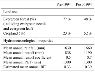
The Nam Muc catchment (2880 km2) is located in the Red River Basin, the second largest drainage basin in Vietnam which also drains parts of China and Laos. The local climate is tropical-monsoon-dominated with distinct wet (May to October) and dry (November to April) seasons. The wet season tends to have high temperatures (on average 27 to 29 ∘C) due to south–southeasterly winds that bring humid air masses. Conversely, during the dry season, circulation patterns reverse carrying cooler dry air masses to the basin (leading to average temperatures of 16 to 21 ∘C). The streamflow response is consequently monsoon-driven, with high flows occurring between June and October (generally peaking in July and August) and low flows in the December to May period (Vu, 1993). Average annual rainfall at Nam Muc varies between 1300 and 2000 mm (on average 1600 mm) and catchment elevation ranges between 350 and 1500 m a.s.l. A summary of catchment properties is provided in Table 1 for pre-change (prior to 1994) and post-change (after 1994) conditions. This separation was based on available land cover information as described below.
2.1 Data and land cover change
Figure 1 shows the available land cover information for the Nam Muc catchment. Land cover information for the catchment is scant; we were able to locate only two sources which unfortunately do not give a complete picture over the entire time period of interest (1970 to 2004). The first land cover map refers to the period 1981–1994 and was obtained by the Vietnamese Forest Inventory and Planning Institute (http://fipi.vn/Home-en.htm). The second land cover map refers to the year 2000 and was obtained from the FAO Global Land Cover database (http://www.fao.org/geonetwork/srv/en/metadata.show?id=12749&currTab=simple). A comparison of the two maps shows a reduction in forest cover in favor of cropland; evergreen leaf decreases from about 60 to 30 %, while cropland increases from about 23 to 52 %. The change in land cover is patchy, although mostly concentrated in the northern part of the catchment. Because of the scant information available, it is not easy to identify the precise time period of these changes. Based on the available land cover map information and the changes to observed runoff (see Sect. 2.2), we posit that a period of rapid extensive deforestation occurred in the early to mid-1990s.
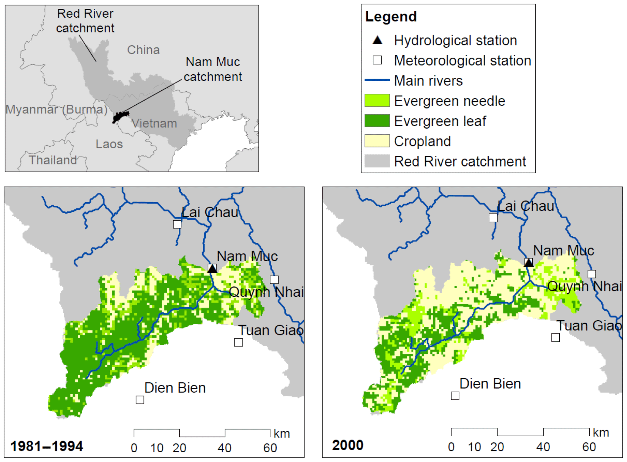
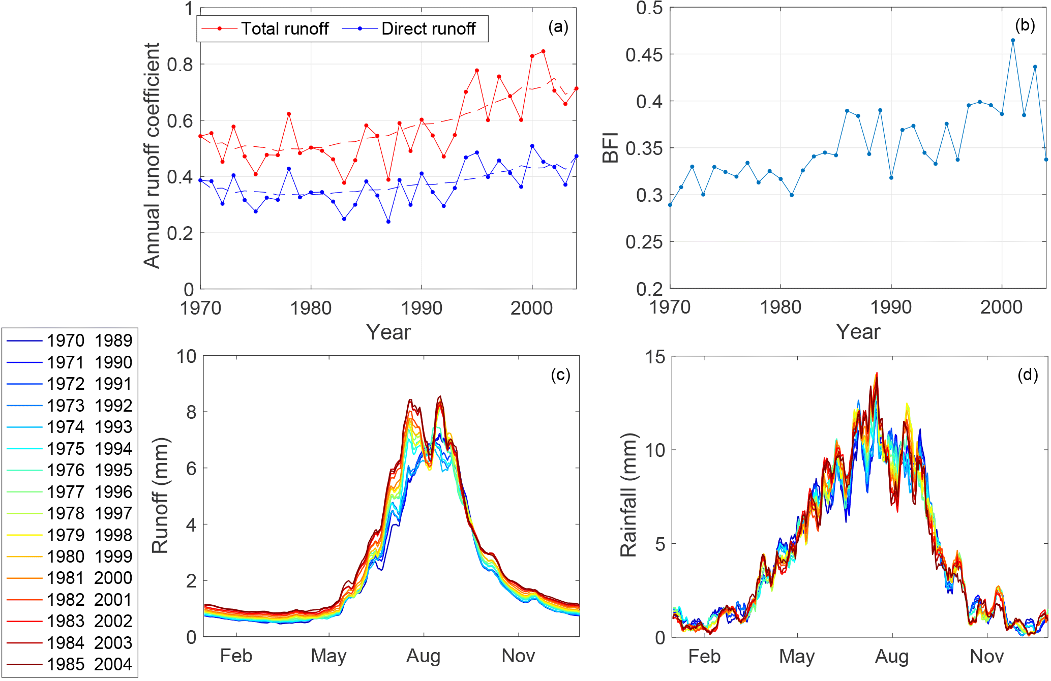
Figure 2Impact of land use change on observed streamflow: (a) annual runoff coefficient, (b) annual baseflow index (BFI), (c) Moving Average over Shifting Horizon (MASH) results for total observed runoff and (d) MASH for observed rainfall.
Daily point rainfall data are available at four precipitation stations surrounding the catchment (Dien Bien, Tuan Giao, Quynh Nhai and Nam Muc; see Fig. 1). Catchment-averaged rainfall was developed as a weighted sum of the four stations with weights determined by Thiessen polygons. Daily mean temperature was calculated in a similar fashion using temperature records from the two closest gauges (Lai Chau and Quynh Nhai; see Fig. 1). This was used to estimate potential evapotranspiration (PET) through the empirical temperature–latitude-based Hamon PET method (Hamon, 1961). Daily rainfall, temperature and streamflow data were provided by the Vietnamese Institute of Water Resources Planning.
2.2 Impact of land cover change on streamflow
The annual runoff and direct runoff coefficient and baseflow index were used to assess the impact of land cover change on the hydrologic regime. Baseflow was estimated using the two-parameter recursive baseflow filter of Eckhardt (2005) (see Eq. 1), with online updating of baseflow estimates to match low flows:
where bk is the estimated baseflow at time k, yk is the total observed streamflow at time k, BFImax is the maximum value of the BFI (long-term ratio of baseflow to total streamflow) and a is a filter parameter. In this study, we adopt BFImax=0.5 and a=0.988 based on manual optimization.
An examination of the observed streamflow and rainfall records shows that distinct changes to the hydrologic regime are evident after the mid-1990s. The annual runoff coefficient varies between 0.4 and 0.6 prior to 1994, after which it increases to between 0.6 and 0.8 until 2004 (see Fig. 2a). However, increases in annual yields are driven mostly by changes to baseflow volume. This is evident in Fig. 2a, which shows that the increase in the annual direct runoff coefficient is less than the increase in the total runoff coefficient (roughly 0.1 increase compared to 0.2 respectively). A small increase in the annual baseflow index is also apparent, from about 0.32 on average in the period 1970 to 1982 to 0.39 on average after 1994 (Fig. 2b). This indicates that the annual increases in baseflow volume exceed the increases in direct runoff volume. Similar changes were found by Wang et al. (2012) who analyzed records in the entire Da River basin, which drains the largest river in the Red River catchment. The exact physical processes behind the observed increase in baseflow are not precisely known, particularly since the effects of land use change from forest to cropland are not unequivocal (Price, 2011). Deforestation may be associated with an increase in mean annual flow and baseflow because of lower interception and evapotranspiration rates (e.g., Keppeler and Ziemer, 1990). Nevertheless, permanent forest removal may decrease baseflow because of soil compaction and lower infiltration rates (e.g., Zimmermann et al., 2006; Bormann and Klaassen, 2008). Some authors also show that tillage practices, associated with forest conversion to cropland, can increase soil porosity, soil water content and infiltration, thus ultimately contributing to baseflow formation (e.g., Alam et al., 2014).
On a seasonal timescale, it is apparent that both wet and dry season flows exhibit temporal variations. We utilized the Moving Average over Shifting Horizon (MASH) (Anghileri et al., 2014) and Mann–Kendall test to assess seasonal trends in observed streamflow, precipitation and temperature data. The MASH tool can be used to qualitatively assess interannual variations in the seasonal pattern of a variable. It works by calculating a statistic of the data (e.g., mean) over the same block of days in consecutive years. A steady increase in baseflow is again apparent (see February to April in Fig. 2c), as well as increases in wet season flows (see June to September in Fig. 2c). The Mann–Kendall test (with significance level equal to 5 %) on annual and monthly streamflow time series shows increasing trends in almost all months, i.e., from October to July. No concurrent increases are apparent in rainfall (see Fig. 2d). Also, the Mann–Kendall test applied to precipitation time series does not show any statistically significant trend, except a decrease in September for Nam Muc and Quynh Nhai stations and an increase in July for the Dien Bien station. Temperature variations are not evident from the MASH analysis (not shown) and no significant trend can be detected by applying the Mann–Kendall test. These results indicate that changes in streamflow dynamics are likely due to land use change rather than climatic impacts.
3.1 Hydrologic models
Conceptual lumped models operating at a daily time step were adopted due to the availability of point rather than distributed hydrometeorological data of sufficient length. We considered the HyMOD (Boyle, 2001) and Hydrologiska Byrans Vattenbalansavdelning (HBV) (Bergström, 1995) models. They differ mainly in the way components of the response flow are separated (HBV has near-surface flow, interflow and baseflow components, while HyMOD has a quick flow and slow flow component only) and how these flows are routed. A schematic of the models is shown in Fig. 3.
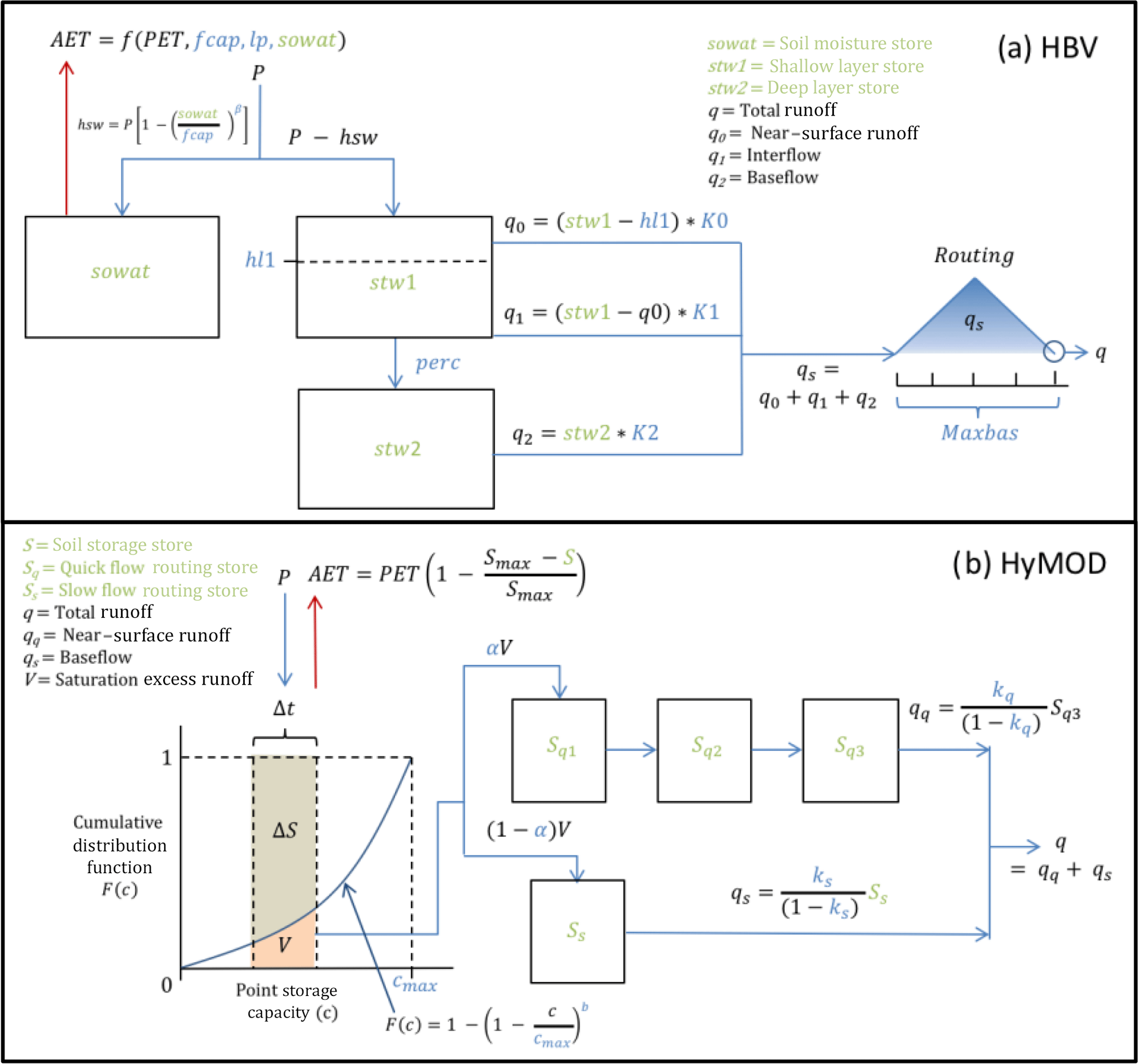
Figure 3Schematic of the models used in this study: (a) HBV and (b) HyMOD. Parameters are shown in blue and states are shown in green.
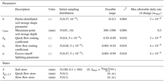
In the HyMOD model, spatial variations in catchment soil storage capacity are represented by a Pareto distribution with shape parameter b and maximum point soil storage depth cmax. Excess rainfall (V) is partitioned into three cascading tanks, representing quick flow and a single slow flow store through the splitting parameter α. Outflow from these linear routing tanks is controlled by parameters kq (for the quick flow store) and ks (for the slow flow store). The model has a total of five states and five parameters.
In the HBV model, input to the soil store is represented by a power-law function (see Fig. 3; note the snow store is neglected for this study). Excess rainfall enters a shallow layer store which generates (1) near-surface flow (q0) whenever the shallow store state (stw1) is above a threshold (hl1) and (2) interflow (q1) through a linear routing mechanism controlled by the K1 parameter. Percolation from the shallow layer store to the deep layer store (controlled by the perc parameter) then leads to the generation of baseflow, also via linear routing (controlled by the K2 parameter). Finally, a triangular weighting function of base length, Maxbas, is used to route the sum of all three flow components. There are a total of nine parameters and three states.
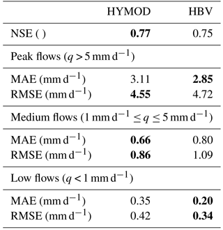
The Shuffled Complex Evolution Algorithm (SCE-UA) (Duan et al., 1993) was used to calibrate HyMOD and the Borg Evolutionary Algorithm (Hadka and Reed, 2013) was used to calibrate HBV. The calibration algorithms were selected based on previous studies that had successfully used them for calibration of these models (Reed et al., 2013; Moradkhani et al., 2005). The calibration procedure itself is however not critical in our study because the optimal parameter values are only used as initial values for the time-varying parameter method. Both models were calibrated to pre-change conditions. The period 1973 to 1979 was selected for calibration (with 2 years for spin-up) as it was expected to have minimal land cover changes (and is therefore representative of pre-change conditions) and also to ensure sufficient data on pre-change conditions are available for assimilation. Both models had very similar performance in terms of reproducing observed runoff (a Nash–Sutcliffe efficiency of 0.75 and 0.77 for HyMOD and HBV respectively). HBV was slightly better at reproducing low flows, while HyMOD was slightly better at mid-range flows (see Table 2). Here the low flow threshold was defined as the average annual 50th percentile flow and the high flow threshold as the average annual 85th percentile flow.
Table 2Model performance in pre-change conditions used for calibration (1975–1979). Boldface numbers correspond to the model with superior performance for the particular metric. NSE is the Nash–Sutcliffe efficiency; MAE is the mean absolute error; RMSE is the root mean squared error.
3.2 Time-varying parameter estimation
A data-assimilation-based framework for estimating time-varying parameters was presented in Pathiraja et al. (2016a). The approach relies on an ensemble Kalman filter (EnKF) (Evensen, 1994) to perform sequential joint state and parameter updating. EnKFs were developed to extend the applicability of the celebrated Kalman filter (Kalman, 1960) to nonlinear systems, although they provide a suboptimal update as only the mean and covariance are considered in generating the posterior distribution. However, they have been used with much success in many hydrologic applications (see for example Reichle et al., 2002; Gu and Oliver, 2005; Komma et al., 2008; Sun et al., 2009; Xu et al., 2016). EnKFs offer a practical alternative to sequential Monte Carlo/particle filter methods that propagate the full probability density through time but suffer from several implementation issues, even in moderate dimensional systems. The LL Dual EnKF method of Pathiraja et al. (2016a) works by sequentially proposing parameters, updating these using the ensemble Kalman filter and available observations and subsequently using these updated parameters to propose and update model states. An approach for proposing parameters in the time-varying setting was also presented, for cases where no prior knowledge of parameter variations is available. The method was verified against multiple synthetic case studies as well as for two small experimental catchments experiencing controlled land use change (Pathiraja et al., 2016a, b). The algorithm is summarized below; for full details refer to Pathiraja et al. (2016a).
3.2.1 LL Dual EnKF
Suppose a dynamical system can be described by a vector of states xt and outputs yt and a vector of associated model parameters θt at any given time t. The uncertain system states and parameters are represented by an ensemble of states and parameters each with n members. The prior state and parameter distributions and , respectively, represent our prior knowledge of the system, usually derived as the output from a numerical model. Suppose also that the system outputs are observed but that there is also some uncertainty associated with these observations. The purpose of the data assimilation algorithm (here the EnKF) is to combine the prior estimates with measurements, based on their respective uncertainties, to obtain an improved estimate of the system states and parameters. A single cycle of the LL Dual EnKF procedure for a given time t is undertaken as follows. Note that in the following, the overbar notation is used to indicate the ensemble mean.
-
Propose a prior parameter ensemble. This involves generating a parameter ensemble using prior knowledge. In this case, our prior knowledge comes from the updated parameter ensemble from the previous time ( and how it has changed over recent time steps. The assumed parameter dynamics is a Gaussian random walk with time-varying mean and variance, given by
where is the sample covariance matrix of the updated parameter ensemble at time t−1; indicates the ensemble mean of the updated parameters at time t−1; ()T represents the transpose operator; and s2 is a tuning parameter. The prior ensemble mean is determined as the linear extrapolation of the updated ensemble means from the previous two time steps; i.e.,
where mt[k] indicates the kth component of the vector mt, the estimated rate of change. Note that the extrapolation is forced to be less than a predefined maximum rate of change mmax to minimize overfitting and avoid parameter drift due to isolated large updates. The maximum rate of change is model-specific and will depend on the modeler's judgement regarding expected extreme changes.
-
Consider observation and forcing uncertainty. This is done by perturbing measurements of forcings and system outputs with random noise sampled from a distribution representing the uncertainty in those measurements. The result is an ensemble of forcings ( and observations ( each with n members. For example, if random errors in measurements of system outputs (herein also referred to as observations) are characterized by a zero mean Gaussian distribution, the ensemble of observations is given by
where is the recorded measurement at time t and is the error covariance matrix of the measurements.
-
Generate simulations using prior parameters. The prior parameters from Step 1, , and updated states from the previous time, , are forced through the model equations to generate an ensemble of model simulations of states ( and outputs (:
-
Perform the Kalman update of parameters. Parameters are updated using the Kalman update equation and the prior parameter and simulated output ensemble from Step 1 and 3:
where is a matrix of the sample cross-covariance between errors in parameters and simulated output ; and is the sample error covariance matrix of the simulated output:
-
Generate simulations using updated parameters. Step 3 is repeated with the updated parameter ensemble to generate the prior ensemble of model simulations of states ( and outputs (:
-
Perform the Kalman update of states and outputs. Use the Kalman update equation for correlated measurement and process noise (Eqs. 15 to 18) and the simulated state ( and output ( ensembles from Step 5 to update them. Since the measurements have already been used to generate , the errors in model simulations and measurements are now correlated. The standard Kalman update equation (as in the form of Eqs. 10 and 11) can no longer be used as it relies on the assumption that errors in measurements and model simulations are independent.
where is a matrix of the sample cross-covariance between simulated states and outputs from Step 5; represents the sample covariance between and the observations; and represents the sample covariance between the and the observations.
The above algorithm specifies the updating of states and parameters at any given time, based on available observations. This allows one to retrospectively estimate time variations in model parameters, as well as provide one-time-step-ahead forecasts of states and outputs (as per Eqs. 8 and 9). Forecasts at longer time horizons (i.e., longer than one time step ahead) would be made by generating prior parameters and states as detailed in Steps 1 to 3, although the local linear extrapolations are only valid close to the current time point.
3.2.2 Application to the Nam Muc catchment
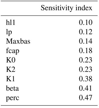
Joint state and parameter estimation was undertaken for the Nam Muc catchment over the period 1980 to 2004 by assimilating streamflow observations into the HyMOD and HBV models at a daily time step. Additionally, simulations using the time-invariant parameters obtained from calibration over the period 1973–1979 were generated for 1980 to 2004, for comparison. Estimating a large number of parameters from limited data is problematic in that the system is highly under-determined, making it difficult to ensure the estimated parameters are meaningful. Given the fairly low parameter dimensionality of HyMOD, all model parameters were allowed to vary in time, while for HBV we applied the Sobol method to identify the most sensitive parameters to be included in the time-varying parameter estimation. The Sobol method is a global sensitivity analysis method based on variance decomposition. It identifies the partial variance contribution of each parameter to the total variance of the hydrological model output (see for example Saltelli et al., 2008; Nossent et al. 2011). The method, implemented through the SAFE toolbox (Pianosi et al., 2015), found the lp and Maxbas parameters to be the least sensitive and least important in defining variations in catchment hydrology (see Table 3). These were held fixed (lp = 1 and Maxbas = 1 day) in the following analysis. Note that although the hl1 parameter was found to have low sensitivity, it was retained as a time-varying parameter due to its conceptual importance in separating interflow and near-surface flow (refer Fig. 3).
Table 3Variance-based sensitivity analysis results for HBV parameters: first-order sensitivity index representing the contribution of varying a single parameter to the variance of the model output. Lower values indicate lower sensitivity.
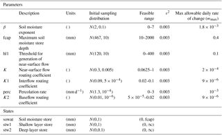
Unbiased normally distributed ensembles of the parameters and states are required to initialize the LL Dual EnKF. Initial parameter ensembles were generated by sampling from a Gaussian distribution with a mean equal to the calibrated parameters over the pre-change period and variance estimated from parameter sets with similar objective function values. Parameter sets with similar objective function values were obtained when using different starting points to the optimization algorithm during the model calibration stage. Initial state ensembles were also sampled from normal distributions with a mean equal to the simulated state at the end of the calibration period. An ensemble size of 100 members was adopted and assumed sufficiently large based on the findings of Moradkhani et al. (2005) and Aksoy et al. (2006). Due to the stochastic–dynamic nature of the method, ensemble statistics were calculated over 20 separate realizations of the LL Dual EnKF. The prior parameter-generating method described in Step 1 of Sect. 3.2 requires specification of the tuning parameter s2 to define the variance of the perturbations. This was tuned by selecting the s2 value that optimized the quality of forecast streamflow over the calibration period. Forecast quality was assessed using the logarithmic score (LS) (Good, 1952) of background streamflow predictions ( using updated parameters (Eq. 15), which was averaged over the calibration period of length T:
where f(y) is the probability density function of the background streamflow predictions (represented by the empirical probability density function of the sample points ; and is the measurement of the system outputs. The s2 value that gave the largest was adopted for the assimilation period. The maximum allowable daily rate of change in the ensemble mean was based on assuming a linear rate of change within the entire feasible parameter space over a 3-year period.
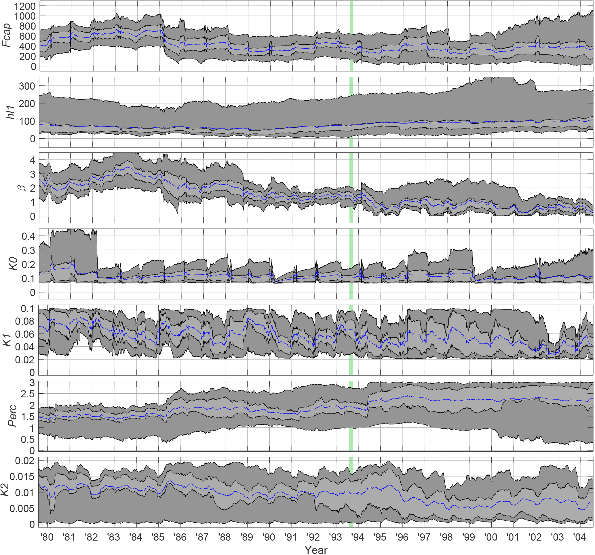
Figure 4Parameter trajectories using the HBV model. The dark grey shaded areas indicate the middle 90 % of the ensemble, bounded by the 5th and 95th percentiles. The light grey shaded areas indicate the middle 50 % of the ensemble, bounded by the 25th and 75th percentiles. The ensemble mean is indicated by the blue line. The vertical green panel indicates the assumed time period of rapid deforestation.
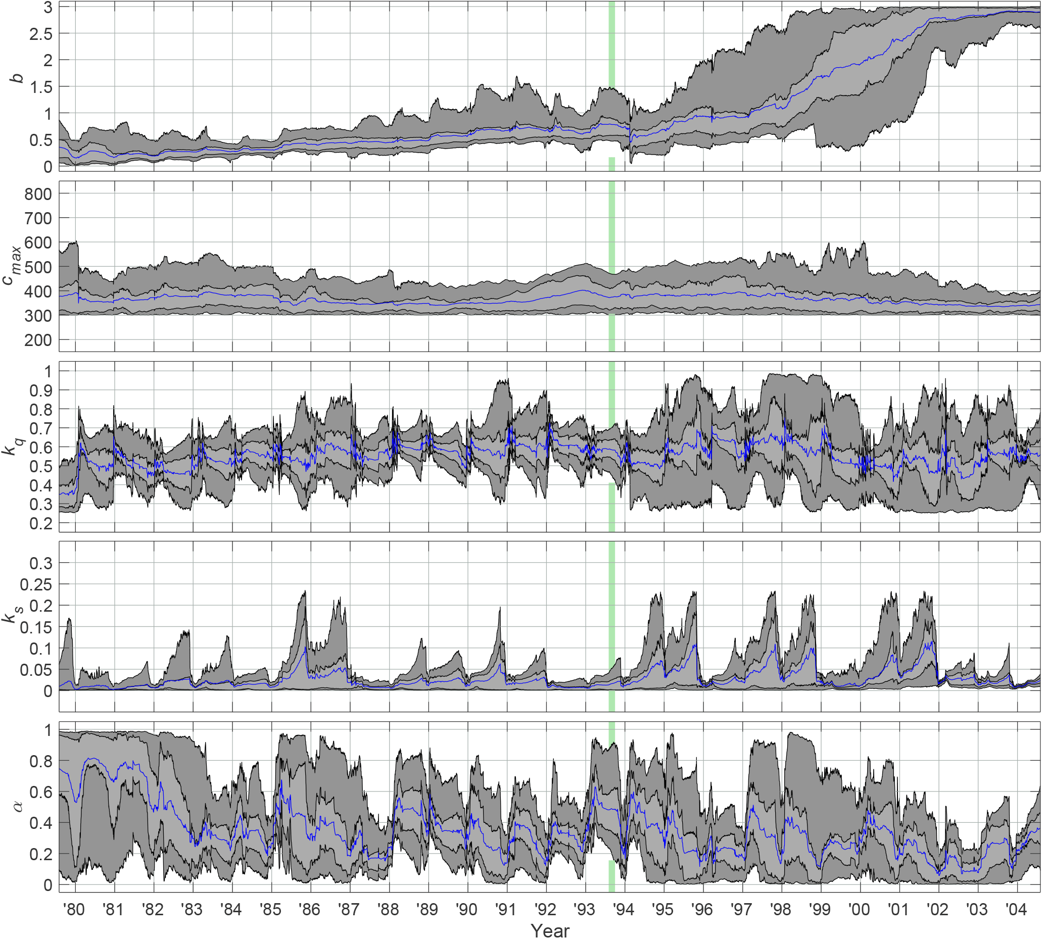
Figure 5Parameter trajectories using the HyMOD model. The dark grey shaded areas indicate the middle 90 % of the ensemble, bounded by the 5th and 95th percentiles. The light grey shaded areas indicate the middle 50 % of the ensemble, bounded by the 25th and 75th percentiles. The ensemble mean is indicated by the blue line. The vertical green panel indicates the assumed time period of rapid deforestation.
As detailed in Sect. 3.2, observation and forcing uncertainty is considered by perturbing measurements with random noise. Here streamflow errors were assumed to be zero-mean normally distributed (truncated to ensure positivity) and heteroscedastic. The variance is defined as a proportion of the observed streamflow, to reflect the fact that larger flows tend to have greater errors than low flows:
where TN indicates the truncated normal distribution to ensure positive flows and d= 0.1. A multiplier of 0.1 was chosen based on estimates adopted for similar gauges in hydrologic data assimilation (DA) studies (e.g., Clark et al., 2008; Weerts and El Serafy, 2006; Xie et al., 2014).
Several studies have noted that a major source of rainfall uncertainty arises from scaling point rainfall to the catchment scale (Villarini and Krajewski, 2008; McMillan et al., 2011) and that multiplicative error models are suited to describing such errors (e.g., Kavetski et al., 2006). Rainfall uncertainties were therefore described using unbiased, lognormally distributed multipliers:
where Pt is the measured rainfall at time t; m and v are the mean and variance of the lognormally distributed rainfall multipliers M, respectively; and μ and σ2 are the mean and variance of the normally distributed logarithm of the rainfall multipliers M. For unbiased perturbations, we let m= 1. The variance of the rainfall multipliers (v) was estimated by considering upper and lower bound error estimates in the Thiessen weights assigned to the four rainfall stations (see Sect. 2.1 for calculation of catchment-averaged rainfall, Pt). The resulting upper and lower bound catchment-averaged rainfall data were then used to estimate error parameters due to spatial variation in rainfall:
where Pupper,10 indicates catchment-averaged rainfall data estimated using the upper bound Thiessen weights with daily depth greater than 10 mm (similar for Plower,10). A 10 mm rainfall depth threshold was chosen to avoid large rainfall fractions due to small rainfall depths. was found to be 0.05 in this case study. Similarly, we assume the dominant source of uncertainty in temperature data arises from spatial variation. Differences in temperature records at Lai Chau and Quynh Nhai (only available gauges with temperature records) were analyzed and found to be approximately normally distributed with a sample mean of 0.2 ∘C and variance of 1.4 ∘C. A perturbed temperature ensemble was then generated according to Eq. (28):
where represents catchment-averaged temperature data (see Sect. 2.1). Note that perturbations were taken to be unbiased (zero mean) as the sample mean of the differences in the temperature records was close to zero. The same perturbed input and observation sequences were used for the HyMOD and HBV runs for the sake of comparison. A summary of the values adopted for the various components of the LL Dual EnKF for each model is provided in Tables 4 and 5.

Figure 6Representative hydrographs of background streamflow from the LL Dual EnKF (black line), time-varying parameter model with no state updating (blue line), time-invariant parameter model with no DA (green line) and observed streamflow (red line). Results for HBV are shown in the top row and HyMOD in the bottom row. A pre-change year (1974) is shown on the left and a post-change year (1998) on the right.
Temporal variations in the estimated parameter distributions from the LL Dual EnKF are evident for both models (see Figs. 4 and 5). In the case of the HBV model, changes on an interannual timescale are evident for the perc and β parameters (see Fig. 4). The decrease in the β parameter means that a greater proportion of rainfall is converted to runoff (i.e., more water entering the shallow layer storage). Additionally, the increase in the perc parameter means that a greater volume of water is made available for baseflow generation. These changes correspond with the observed increase in the annual runoff coefficient (Fig. 2) and increase in baseflow volume (as discussed in Sect. 2.2). From an algorithm perspective, these parameters are most strongly correlated with streamflow (as well as the most sensitive; see Table 3), meaning that they will receive the greatest proportional updates. Similar parameter adjustments are seen for HyMOD, at least at a qualitative level (see Fig. 5). The sharp increase in the b parameter during the post-change period means that a greater volume of water is available for routing (as larger b values mean that a smaller proportion of the catchment has deep soil storage capacity) and the downward interannual trend in α means that a greater portion of excess runoff is routed through the baseflow store. Intra-annual variations in updated model parameters for both HyMOD and HBV are also apparent (refer Figs. 4 and 5). This is due to the inability of a single parameter distribution to accurately model both wet and dry season flows. Such variations were not observed when using the time-varying parameter framework for small deforested catchments (< 350 ha) (see Pathiraja et al., 2016b). The comparatively less clear parameter changes for the Nam Muc catchment are due to a combination of the increased difficulty in accurately modeling the hydrologic response (even in pre-change conditions) and due to the relatively more subtle and gradual changes to land cover. Nonetheless, the method is shown to generate a temporally varying structure that is conceptually representative of the observed changes.
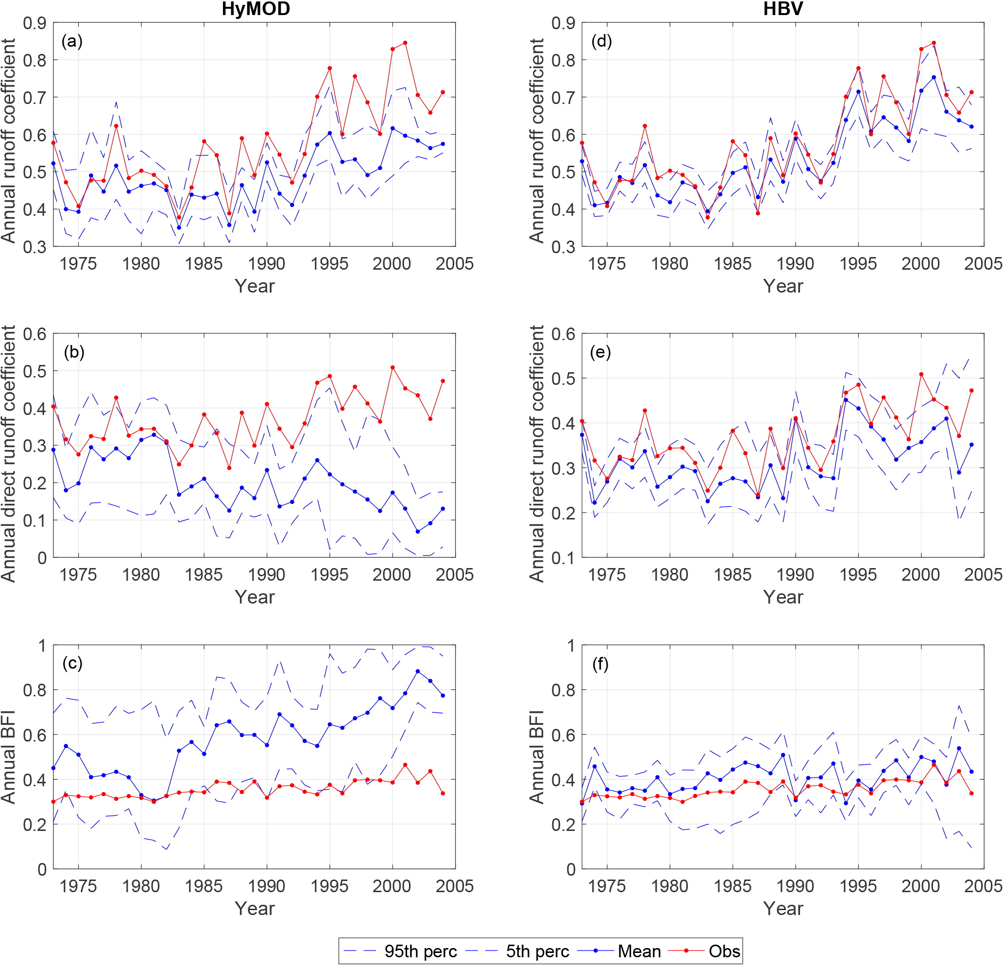
Figure 7Influence of time-varying parameters on model output (i.e., without state updating) summarized in terms of the annual runoff coefficient (top row), annual direct runoff coefficient (second row) and annual baseflow index (BFI) (third row). Results for HyMOD are shown in the first column, and results for HBV are shown in the second column.
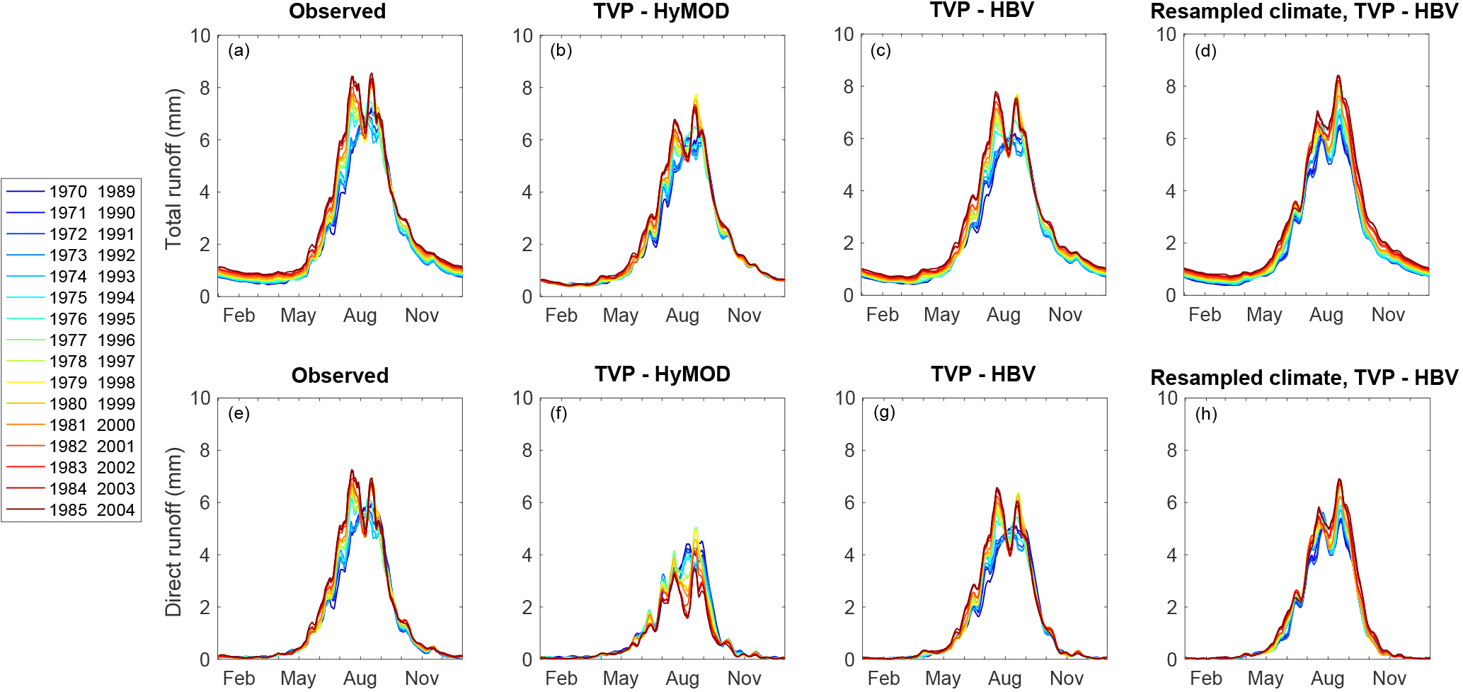
Figure 8Moving Average over Shifting Horizon (MASH) results for observed streamflow (first column), simulated streamflow from time-varying parameter model (without state DA) for HYMOD (second column), HBV (third column) and resampled climate HBV (fourth column). These are split into total runoff (first row) and direct runoff or surface runoff (second row).
Despite the overall correspondence between changes to model parameters and observed streamflow, a closer examination shows that the hydrologic model structure is critical in determining whether the time-varying parameter models accurately reflect changes in all aspects of the hydrologic response (not just total streamflow). In order to examine the impact of parameter variations on the model dynamics, we generated model simulations with the time-varying parameter ensemble from the LL Dual EnKF, but without state updating (hereafter referred to as TVP-HBV and TVP-HyMOD). Streamflow predictions from the LL Dual EnKF (i.e., with state and parameter updating) for both the HyMOD and HBV are generally of similar quality and superior to those from the respective time-invariant parameter models that have been calibrated on pre-change data (1975–1979), although a slight bias in baseflow predictions from HyMOD is evident (see for example Fig. 6). The Nash–Sutcliffe efficiency of one-step-ahead streamflow predictions over the period 1980–2004 from the LL Dual EnKF is 0.87 when using HyMOD or HBV, compared to 0.76 and 0.72 for the respective time-invariant parameter models evaluated over the same period. However, differences in predictions from TVP-HBV and TVP-HyMOD are more striking due to the lack of state updating. Figure 7 shows annual statistics of simulated streamflow from the TVP-HBV and TVP-HyMOD models and observed runoff. The TVP-HBV gives direct runoff and baseflow predictions that are consistent with runoff observations, meaning that the parameter adjustments reflect the observed changes in the runoff response. This however is not the case for the TVP-HyMOD. The annual runoff coefficient and annual direct runoff coefficient are severely underestimated in the post-change period by the TVP-HyMOD, while the annual baseflow index has an increasing trend of magnitude far greater than that observed (Fig. 7c). All three quantities on the other hand are well represented by the TVP-HBV (Fig. 7d–f). Similar conclusions can be drawn from Fig. 8, which shows the results of a Moving Average over Shifting Horizon (MASH) analysis (see Sect. 2.2) on total and direct runoff (observed and simulated). Observed increases in January to April flows (see Fig. 8a) and wet season direct flows (July to September) (see Fig. 8e) are well represented by the TVP-HBV but not TVP-HyMOD.
The reason for the differences in performance between the TVP-HBV and TVP-HyMOD lies in the structure of the hydrologic model. The TVP-HyMOD is incapable of representing the observed increase in annual runoff/direct runoff coefficient due to the increased baseflow during dry periods, despite having an annual baseflow index far greater than the observed. This occurs due to an inability to generate flow volume during periods of no rain. In joint state–parameter updating using HyMOD, underestimated runoff predictions during dry periods lead to adjustments to the ks and α parameters to increase baseflow depth (since these are the only parameters that are associated with an active store). Unlike HBV, HyMOD has no continuous supply of water to the routing stores (i.e., the quick flow and slow flow stores) during recession periods (which typically have extended periods of no rainfall, so that V in Fig. 3 is zero). This means that ks and α are updated to extreme values to compensate for the volumetric shortfall. The HBV structure, on the other hand, has a continuous percolation of water into the deep layer store even during periods of no rain (as long as the shallow water store is non-empty). In summary, the HyMOD model structure is poorly suited to simulating streamflow dynamics in post-change conditions, although it gave reasonable simulations in pre-change conditions. This highlights the need to select a sufficiently flexible model structure prior to undertaking forecasting or predictive modeling using the time-varying parameter approach. In particular, the model structure must be capable of effectively simulating all potential future catchment conditions.
Having established that the TVP-HBV provided a good representation of the observed streamflow dynamics, we used a modeling approach to determine whether the observed changes were solely driven by forcings and which (if any) components of runoff were also affected by land use change. A resampled rainfall and temperature time series was generated by sampling the data without replacement across years for each day (for instance rainfall and temperature for 1 January 1990 is found by randomly sampling from all records on 1 January). This maintains the intra-annual (e.g., seasonal) variability but destroys any interannual trends in the meteorological data. Streamflow simulations were then generated using this resampled meteorological sequence as inputs to the TVP-HBV (i.e., without state updating). If the resulting streamflow simulations do not reproduce the observed changes to streamflow dynamics, then this indicates that changes to meteorological forcings are the main contributor. However, if it is able to at least partially (or fully) reproduce the observed streamflow changes, this means that land cover changes are impacting catchment hydrology (but potentially in addition to forcing changes, due to the presence of ecosystem feedbacks). Figure 8d and h show the results of a MASH analysis undertaken on the resulting simulations of total and direct runoff using the resampled forcing time series and TVP-HBV model. Observed increases in baseflow during the January–April period (see Fig. 8a) and increases in direct runoff in the June–September period (see Fig. 8e) are reproduced. The magnitude of increase in direct runoff in July is slightly lower, also indicating the potential for some climatic influences. This is consistent with findings from the Mann–Kendall test, which identified a statistically significant increase in July rainfall (see Sect. 2.2). Overall, however, these results give further weight to the conclusion that land cover change has impacted the hydrologic regime of the Nam Muc catchment. These results also demonstrate that parameter changes correspond to actual changes in catchment hydrology and are not just random fluctuations that reproduce the observed streamflow statistics only when the observed forcing time series is used.
As our anthropogenic footprint expands, it will become increasingly important to develop modeling methodologies that are capable of handling changing catchment conditions. Previous work proposed the use of models whose parameters vary with time in response to signals of change in observations. The so-called Locally Linear (LL) Dual EnKF time-varying parameter estimation algorithm (Pathiraja et al., 2016a) was applied to two sets of small (< 350 ha) paired experimental catchments with deforestation occurring under experimental conditions (rapid clearing of 100 and 50 % of land surface) (Pathiraja et al., 2016b). Here we demonstrate the efficacy of the method for a larger catchment experiencing more realistic land cover change, while also investigating the importance of the chosen model structure in ensuring the success of the time-varying parameter estimation method. We also demonstrate that the time-varying parameter framework can be used in a retrospective fashion to determine whether land cover changes (and not just meteorological factors) contribute to the observed hydrologic changes.
Experiments were undertaken in the Nam Muc catchment (2880 km2) in Vietnam, which experienced a relatively gradual conversion from forest to cropland over a number of years (cropland increased from roughly 23 % of the catchment between 1981 and 1994 to 52 % by 2000). Changes to the hydrologic regime after the mid-1990s were detected and attributed mostly to an increase in baseflow volume. Application of the LL Dual EnKF with two conceptual models (HBV and HyMOD) showed that the time-varying parameter framework with state updating improved streamflow prediction in post-change conditions compared to the time-invariant parameter case. However, baseflow predictions from the LL Dual EnKF with HBV were generally superior to the HyMOD case which tended to have a slight negative bias. It was found that the structure (i.e., model equations) of HyMOD was unsuited to representing the modified baseflow conditions, resulting in extreme and unrealistic time-varying parameter estimates. This work shows that the chosen model is critical for ensuring the time-varying parameter framework successfully models streamflow in unknown future land cover conditions, particularly when used in a real-time forecasting mode. Appropriate model selection can be a difficult task due to the significant uncertainty associated with future land use change and can be even more problematic when multiple models have similar performance in pre-change conditions (as was the case in this study). One possible way to ensure success of the time-varying parameter approach is to use models whose fundamental equations explicitly represent key physical processes (for instance, modeling subsurface flow using the Richards equation with hydraulic conductivity allowed to vary with time). In this way, time variations in model parameters would more closely reflect changes to physiographic properties, rather than also having to account for missing processes. The drawback of such physically based models is that they are generally data-intensive, both in generating model simulations (i.e., detailed inputs) and specifying parameters. Additionally, it may be necessary to reduce the dimensionality of the time-varying parameter vector by keeping less sensitive model parameters fixed in order to make the estimation problem tractable. Models of intermediate complexity that have explicit process descriptions may be the most promising, although this also remains to be demonstrated.
The data used in this paper were collected under the project IMRR (Integrated and sustainable water Management of Red Thai Binh Rivers System in changing climate), funded by the Italian Ministry of Foreign Affairs (Delibera no. 142 del 8 Novembre 2010). Data utilized in this study can be made available from the authors upon request.
The authors declare that they have no conflict of interest.
This study was funded by the Australian Research Council as part of the Discovery Project DP140102394. Lucy Marshall is additionally supported through a Future Fellowship FT120100269. The research of Sahani Pathiraja has been partially funded by the Deutsche Forschungsgemeinschaft (DFG) through the grant CRC 1294 “Data Assimilation.”
We greatly acknowledge Andrea Castelletti for provision
of data and for discussions on this work.
Edited by: Markus
Hrachowitz
Reviewed by: Carine Poncelet and two anonymous
referees
Aksoy, A., Zhang, F., and Nielsen-Gammon, J.: Ensemble-Based Simultaneous State and Parameter Estimation in a Two-Dimensional Sea-Breeze Model, Mon. Weather Rev., 134, 2951–2970, 2006.
Alam, M., Islam, M., Salahin, N., and Hasanuzzaman, M.: Effect of tillage practices on soil properties and crop productivity in wheat-mungbean-rice cropping system under subtropical climatic conditions, Sci. World J., 2014, 437283, https://doi.org/10.1155/2014/437283, 2014.
Anghileri, D., Pianosi, F., and Soncini-Sessa, R.: Trend detection in seasonal data: From hydrology to water resources, J. Hydrol., 511, 171–179, https://doi.org/10.1016/j.jhydrol.2014.01.022, 2014.
Bergström, S.: The HBV model, in: Computer Models of Watershed Hydrology, edited by: Singh, V. P., Water Resources Publications, Highlands Ranch, CO, 443–476, 1995.
Bhaduri, B. B., Minner, M., Tatalovich, S., Member, A., and Harbor, J.: Long-term hydrologic impact of urbanization: A tale of two models, J. Water Res. Plan. Man., 127, 13–19, 2001.
Bormann, H. and Klaassen, K.: Seasonal and land use dependent variability of soil hydraulic and soil hydrological properties of two Northern German soils, Geoderma, 145, 295–302, 2008.
Boyle, D.: Multicriteria calibration of hydrological models, PhD dissertation, Univ. of Ariz., Tucson, 2001.
Brown, A. E., Mcmahon, T. A., Podger, G. M., and Zhang, L.: A methodology to predict the impact of changes in forest cover on flow duration curves, CSIRO Land and Water Science Report 8/06, 2006.
Brown, A. E., Western, A. W., McMahon, T. A., and Zhang, L.: Impact of forest cover changes on annual streamflow and flow duration curves, J. Hydrol., 483, 39–50, 2013.
Clark, M. P., Rupp, D. E., Woods, R. A., Zheng, X., Ibbitt, R. P., Slater, A. G., Schmidt, J., and Uddstrom, M. J.: Hydrological data assimilation with the ensemble Kalman filter: Use of streamflow observations to update states in a distributed hydrological model, Adv. Water Resour., 31, 1309–1324, https://doi.org/10.1016/j.advwatres.2008.06.005, 2008.
Coe, M. T., Latrubesse, E. M., Ferreira, M. E., and Amsler, M. L.: The effects of deforestation and climate variability on the streamflow of the Araguaia River, Brazil, Biogeochemistry, 105, 119–131, https://doi.org/10.1007/s10533-011-9582-2, 2011.
Coron, L., Andréassian, V., Perrin, C., Lerat, J., Vaze, J., Bourqui, M., and Hendrickx, F.: Crash testing hydrological models in contrasted climate conditions: An experiment on 216 Australian catchments, Water Resour. Res., 48, 1–17, https://doi.org/10.1029/2011WR011721, 2012.
Costa, M. H., Botta, A., and Cardille, J. A.: Effects of large-scale changes in land cover on the discharge of the Tocantins River, Southeastern Amazonia, J. Hydrol., 283, 206–217, https://doi.org/10.1016/S0022-1694(03)00267-1, 2003.
Duan, Q. Y., Gupta, V. K., and Sorooshian, S.: Shuffled complex evolution approach for effective and efficient global minimization, J. Optimiz. Theory App., 76, 501–521, https://doi.org/10.1007/BF00939380, 1993.
Dwarakish, G. S. and Ganasri, B. P.: Impact of land use change on hydrological systems: A review of current modeling approaches, Cogent Geoscience, 1, 1115691–1115691, https://doi.org/10.1080/23312041.2015.1115691, 2015.
Eckhardt, K.: How to construct recursive digital filters for baseflow separation, Hydrol. Process., 19, 507–515, https://doi.org/10.1002/hyp.5675, 2005.
Efstratiadis, A., Nalbantis, I., and Koutsoyiannis, D.: Hydrological modelling of temporally-varying catchments: facets of change and the value of information, Hydrolog. Sci. J., 60, 1438–1461, https://doi.org/10.1080/02626667.2014.982123, 2015.
Elfert, S. and Bormann, H.: Simulated impact of past and possible future land use changes on the hydrological response of the Northern German lowland “Hunte” catchment, J. Hydrol., 383, 245–255, https://doi.org/10.1016/j.jhydrol.2009.12.040, 2010.
Evensen, G.: Sequential data assimilation with a nonlinear quasi-geostrophic model using Monte Carlo methods to forecast error statistics, J. Geophys. Res., 99, 10143–10162, https://doi.org/10.1029/94JC00572, 1994.
FAO: Global Forest Resources Assessment 2005, FRA, available at: http://www.fao.org/docrep/008/a0400e/a0400e00.htm (last access: June 2017), 2005.
Good, I. J.: Rational Decisions, J. Roy. Stat. Soc. B, 14, 107–114, 1952.
Giuliani, M., Anghileri, D., Castelletti, A., Vu, P. N., and Soncini-Sessa, R.: Large storage operations under climate change: expanding uncertainties and evolving tradeoffs, Environ. Res. Lett., 11, 035009, https://doi.org/10.1088/1748-9326/11/3/035009, 2016.
Gu, Y. and Oliver, D. S.: History matching of the PUNQ-S3 reservoir model using the ensemble Kalman filter, SPE J., 10, 217–224, https://doi.org/10.2118/89942-PA, 2005.
Hadka, D. and Reed, P.: Borg: an auto-adaptive many-objective evolutionary computing framework, Evol. Comput., 21, 231–259, 2013.
Hamon, W.: Estimating potential evapotranspiration, T. Am. Soc. Civ. Eng., 128, 324–337, 1961.
Kalman, R. E.: A new approach to linear filtering and prediction problems, J. Basic Eng.-T ASME, 82, 35–45, 1960.
Kavetski, D., Kuczera, G., and Franks, S. W.: Bayesian analysis of input uncertainty in hydrological modeling: 1. Theory, Water Resour. Res., 42, https://doi.org/10.1029/2005WR004368, 2006.
Keppeler, E. T. and Ziemer, R. R.: Logging effects on streamflow: water yield and summer low flows at Caspar Creek in northwestern California, Water Resour. Res., 26, 1669–1679, 1990.
Kim, D.-H., Sexton, J. O., and Townshend J. R.: Accelerated deforestation in the humid tropics from the 1990s to the 2000s, Geophys. Res. Lett., 42, 3495–3501, https://doi.org/10.1002/ 2014GL062777, 2015.
Komma, J., Blöschl, G., and Reszler, C.: Soil moisture updating by Ensemble Kalman Filtering in real-time flood forecasting, J. Hydrol., 357, 228–242, https://doi.org/10.1016/j.jhydrol.2008.05.020, 2008.
Kummer, D. and Turner, B.: The Human Causes of Deforestation in Southeast Asia, BioScience, 44, 323–328, https://doi.org/10.2307/1312382, 1994.
Legesse, D., Vallet-Coulomb, C., and Gasse, F.: Hydrological response of a catchment to climate and land-use changes in Tropical Africa: case study South Central Ethiopia, J. Hydrol., 275, 67–85, https://doi.org/10.1016/S0022-1694(03)00019-2, 2003.
Marshall, L., Sharma, A., and Nott, D.: Modeling the catchment via mixtures: Issues of model specification and validation, Water Resour. Res., 42, 1–14, https://doi.org/10.1029/2005WR004613, 2006.
McIntyre, N. and Marshall, M.: Identification of rural land management signals in runoff response, Hydrol. Process., 24, 3521–3534, https://doi.org/10.1002/hyp.7774, 2010.
McMillan, H., Jackson, B., Clark, M., Kavetski, D., and Woods, R.: Rainfall uncertainty in hydrological modelling: An evaluation of multiplicative error models, J. Hydrol., 400, 83–94, https://doi.org/10.1016/j.jhydrol.2011.01.026, 2011.
Moradkhani, H., Sorooshian, S., Gupta, H. V., and Houser, P. R.: Dual state–parameter estimation of hydrological models using ensemble Kalman filter, Adv. Water Resour., 28, 135–147, https://doi.org/10.1016/j.advwatres.2004.09.002, 2005.
Niu, J. and Sivakumar, B.: Study of runoff response to land use change in the East River basin in South China, Stoch. Env. Res. Risk A., 28, 857, https://doi.org/10.1007/s00477-013-0690-5, 2013.
Nossent, J., Elsen, P., and Bauwens, W.: Sobol'sensitivity analysis of a complex environmental model, Environ. Modell. Softw., 26, 1515–1525, 2011.
Pathiraja, S., Marshall, L., Sharma, A., and Moradkhani, H.: Hydrologic modeling in dynamic catchments: A data assimilation approach, Water Resour. Res., 52, 3350–3372, https://doi.org/10.1002/2015WR017192, 2016a.
Pathiraja, S., Marshall, L., Sharma, A., and Moradkhani, H.: Detecting non-stationary hydrologic model parameters in a paired catchment system using data assimilation, Adv. Water Resour., 94, 103–119, https://doi.org/10.1016/j.advwatres.2016.04.021, 2016b.
Pianosi, F., Sarrazin, F., and Wagener, T.: A Matlab toolbox for Global Sensitivity Analysis, Environ. Modell. Softw., 70, 80–85, https://doi.org/10.1016/j.envsoft.2015.04.009, 2015.
Price, K.: Effects of watershed topography, soils, land use, and climate on baseflow hydrology in humid regions: A review, Prog. Phys. Geog., 35, 465–492, 2011.
Reed, P. M., Hadka, D., Herman, J. D., Kasprzyk, J. R., and Kollat, J. B.: Evolutionary multiobjective optimization in water resources: The past, present, and future, Adv. Water Resour., 51, 438–456, 2013.
Reichle, R. H., McLaughlin, D. B., and Entekhabi, D.: Hydrologic Data Assimilation with the Ensemble Kalman Filter, Mon. Weather Rev., 130, 103–114, https://doi.org/10.1175/1520-0493(2002)130<0103:HDAWTE>2.0.CO;2, 2002.
Rose, S. and Peters, N. E.: Effects of urbanization on streamflow in the Atlanta area (Georgia, USA): a comparative hydrological approach, Hydrol. Process., 15, 1441–1457, https://doi.org/10.1002/hyp.218, 2001.
Saltelli, A., Ratto, M., Andres, T., Campolongo, F., Cariboni, J., Gatelli, D., Saisana, M., and Tarantola, S.: Global Sensitivity Analysis, the Primer, Wiley, Chichester, England, 2008.
Seibert, J. and McDonnell, J. J.: Land-cover impacts on streamflow: a change-detection modelling approach that incorporates parameter uncertainty, Hydrolog. Sci. J., 55, 316–332, https://doi.org/10.1080/02626661003683264, 2010.
Sun, A. Y., Morris, A., and Mohanty, S.: Comparison of deterministic ensemble Kalman filters for assimilating hydrogeological data, Adv. Water Resour., 32, 280–292, https://doi.org/10.1016/j.advwatres.2008.11.006, 2009.
Taver, V., Johannet, A., Borrell-Estupina, V., and Pistre, S.: Feed-forward vs recurrent neural network models for non-stationarity modelling using data assimilation and adaptivity, Hydrolog. Sci. J., 60, 1242–1265, https://doi.org/10.1080/02626667.2014.967696, 2015.
Thanapakpawin, P., Richey, J., Thomas, D., Rodda, S., Campbell, B., and Logsdon, M.: Effects of landuse change on the hydrologic regime of the Mae Chaem river basin, NW Thailand, J. Hydrol., 334, 215–230, https://doi.org/10.1016/j.jhydrol.2006.10.012, 2007.
Villarini, G. and Krajewski, W. F.: Empirically-based modeling of spatial sampling uncertainties associated with rainfall measurements by rain gauges, Adv. Water Resour., 31, 1015–1023, https://doi.org/10.1016/j.advwatres.2008.04.007, 2008.
Vu, V. T.: Evaluation of the impact of deforestation to inflow regime of the Hoa Binh Reservoir in Vietnam, Hydrology of Warm Humid Regions, Proceedings of the Yokohama Symposium, July 1993, IAHS Publ. no. 216, 1993.
Wang, J., Ishidaira, H., and Xu, Z. X.: Effects of climate change and human activities on inflow into the Hoabinh Reservoir in the Red River basin, Procedia Environ. Sci., 13, 1688–1698, 2012.
Warburton, M. L., Schulze, R. E., and Jewitt, G. P. W.: Hydrological impacts of land use change in three diverse South African catchments, J. Hydrol., 414–415, 118–135, https://doi.org/10.1016/j.jhydrol.2011.10.028, 2012.
Weerts, A. H. and El Serafy, G. Y. H.: Particle filtering and ensemble Kalman filtering for state updating with hydrological conceptual rainfall-runoff models, Water Resour. Res., 42, https://doi.org/10.1029/2005WR004093, 2006.
Westra, S., Thyer, M., Leonard, M., Kavetski, D., and Lambert, M.: A strategy for diagnosing and interpreting hydrological model nonstationarity, Water Resour. Res., 5090–5113, https://doi.org/10.1002/2013WR014719, 2014.
Wijesekara, G. N., Gupta, A., Valeo, C., Hasbani, J. G., Qiao, Y., Delaney, P., and Marceau, D. J.: Assessing the impact of future land-use changes on hydrological processes in the Elbow River watershed in southern Alberta, Canada, J. Hydrol., 412–413, 220–232, https://doi.org/10.1016/j.jhydrol.2011.04.018, 2012.
WWF: Ecosystems in the Greater Mekong: Past trends, current status, possible futures, 2013.
Xie, X., Meng, S., Liang, S., and Yao, Y.: Improving streamflow predictions at ungauged locations with real-time updating: application of an EnKF-based state-parameter estimation strategy, Hydrol. Earth Syst. Sci., 18, 3923–3936, https://doi.org/10.5194/hess-18-3923-2014, 2014.
Xu, T. and Gomez-Hernandez, J.: Joint identification of contaminant source location, initial release time, and initial solute concentration in an aquifer via ensemble kalman filtering, Water Resour. Res., 600–612, https://doi.org/10.1002/2016WR019111, 2016.
Yang, L., Wei, W., Chen, L., and Mo, B.: Response of deep soil moisture to land use and afforestation in the semi-arid Loess Plateau, China, J. Hydrol., 475, 111–122, https://doi.org/10.1016/j.jhydrol.2012.09.041, 2012.
Zimmermann, B., Elsenbeer, H., and De Moraes, J. M.: The influence of land-use changes on soil hydraulic properties: implications for runoff generation, Forest Ecol. Manag., 222, 29–38, 2006.