the Creative Commons Attribution 4.0 License.
the Creative Commons Attribution 4.0 License.
 | 18 May 2018
Groundwater withdrawal in randomly heterogeneous coastal aquifers
Martina Siena
Monica Riva
We analyze the combined effects of aquifer heterogeneity and pumping operations on seawater intrusion (SWI), a phenomenon which is threatening coastal aquifers worldwide. Our investigation is set within a probabilistic framework and relies on a numerical Monte Carlo approach targeting transient variable-density flow and solute transport in a three-dimensional randomly heterogeneous porous domain. The geological setting is patterned after the Argentona river basin, in the Maresme region of Catalonia (Spain). Our numerical study is concerned with exploring the effects of (a) random heterogeneity of the domain on SWI in combination with (b) a variety of groundwater withdrawal schemes. The latter have been designed by varying the screen location along the vertical direction and the distance of the wellbore from the coastline and from the location of the freshwater–saltwater mixing zone which is in place prior to pumping. For each random realization of the aquifer permeability field and for each pumping scheme, a quantitative depiction of SWI phenomena is inferred from an original set of metrics characterizing (a) the inland penetration of the saltwater wedge and (b) the width of the mixing zone across the whole three-dimensional system. Our results indicate that the stochastic nature of the system heterogeneity significantly affects the statistical description of the main features of the seawater wedge either in the presence or in the absence of pumping, yielding a general reduction of toe penetration and an increase of the width of the mixing zone. Simultaneous extraction of fresh and saltwater from two screens along the same wellbore located, prior to pumping, within the freshwater–saltwater mixing zone is effective in limiting SWI in the context of groundwater resources exploitation.


Groundwater resources in coastal aquifers are seriously threatened by seawater intrusion (SWI), which can deteriorate the quality of freshwater aquifers, thus limiting their potential use. This situation is particularly exacerbated within areas with intense anthropogenic activities, which are associated with competitive uses of groundwater in connection, e.g., with agricultural processes, industrial processes and/or high urban water supply demand. Critical SWI scenarios are attained when seawater reaches extraction wells designed for urban freshwater supply, with severe environmental, social and economic implications (e.g., Custodio, 2010; Mas-Pla et al., 2014; Mazi et al., 2014).
The development of effective strategies for sustainable use of groundwater resources in coastal regions should be based on a comprehensive understanding of SWI phenomena. This challenging problem has been originally studied by assuming a static equilibrium between freshwater (FW) and seawater (SW) and a sharp FW–SW interface, where FW and SW are considered as immiscible fluids. Under these hypotheses, the vertical position of the FW–SW interface below the sea level, z, is given by the Ghyben–Herzberg solution, , where hF is the FW head above sea level and is the density contrast, ρS and ρF, respectively, being SW and FW density. Starting from these works, several analytical and semi-analytical expressions have been developed to describe SWI under diverse flow configurations (e.g., Strack, 1976; Dagan and Zeitoun, 1998; Bruggeman, 1999; Cheng et al., 2000; Bakker, 2006; Nordbotten and Celia, 2006; Park et al., 2009). In this broad context, Strack (1976) evaluated the maximum (or critical) pumping rate to avoid encroachment of SW in FW pumping wells. All of these sharp-interface-based solutions neglect a key aspect of SWI phenomena, i.e., the formation of a transition zone where mixing between FW and SW takes place and fluid density varies with salt concentration. As a consequence, these models may significantly overestimate the actual penetration length of the SW wedge, leading to an excessively conservative evaluation of the critical pumping rate (Gingerich and Voss, 2005; Pool and Carrera, 2011; Llopis-Albert and Pulido-Velazquez, 2013).
A more realistic approach relies on the formulation and solution of a variable-density problem, in which SW and FW are considered as miscible fluids and groundwater density depends on salt concentration. The complexity of the problem typically prevents finding a solution via analytical or semi-analytical methods, with a few notable exceptions (Henry, 1964; Dentz et al., 2006; Bolster et al., 2007; Zidane et al., 2012; Fahs et al., 2014). Henry (1964) developed a semi-analytical solution for a variable-density diffusion problem in a (vertical) two-dimensional homogeneous and isotropic domain. Dentz et al. (2006) and Bolster et al. (2007) applied perturbation techniques to solve analytically the Henry problem for a range of (small and intermediate) values of the Péclet number, which characterizes the relative strength of convective and dispersive transport mechanisms. Zidane et al. (2012) solved the Henry problem for realistic (small) values of the diffusion coefficient. Finally, Fahs et al. (2014) presented a semi-analytical solution for a square porous cavity system subject to diverse salt concentrations at its vertical walls. Practical applicability of these solutions is quite limited, due to their markedly simplified characteristics. Various numerical codes have been proposed to solve variable-density flow and transport equations (e.g., Voss and Provost, 2002; Ackerer et al., 2004; Soto Meca et al., 2007; Ackerer and Younes, 2008; Albets-Chico and Kassinos, 2013). Numerical simulations can provide valuable insights into the effects of dispersion on SWI, a feature that is typically neglected in analytical and semi-analytical solutions. Abarca et al. (2007) introduced a modified Henry problem to account for dispersive solute transport and anisotropy in hydraulic conductivity. Kerrou and Renard (2010) analyzed the dispersive Henry problem within two- and three-dimensional randomly heterogeneous aquifer systems. These authors relied on computational analyses performed on a single three-dimensional realization, invoking ergodicity assumptions. Lu et al. (2013) performed a set of laboratory experiments and numerical simulations to investigate the effect of geological stratification on SW–FW mixing. Riva et al. (2015) considered the same setting as in Abarca et al. (2007) and studied the way quantification of uncertainty associated with SWI features is influenced by lack of knowledge of four key dimensionless parameters controlling the process, i.e., gravity number, permeability anisotropy ratio and transverse and longitudinal Péclet numbers. Enhancement of mixing in the presence of tidal fluctuations and/or FW table oscillations has been analyzed by Ataie-Ashtiani et al. (1999), Lu et al. (2009, 2015) and Pool et al. (2014) in homogeneous aquifers and by Pool et al. (2015) in randomly heterogeneous three-dimensional systems (under ergodic conditions). Recent reviews on the topic are offered by Werner et al. (2013) and Ketabchi et al. (2016).
Several numerical modeling studies have been performed with the aim of identifying the most effective strategy for the exploitation of groundwater resources in domains mimicking the behavior of specific sites. Dausman and Langevin (2005) examined the influence of hydrologic stresses and water management practices on SWI in a superficial aquifer (Broward County, USA) by developing a variable-density model formed by two homogeneous hydrogeological units. Werner and Gallagher (2006) studied SWI in the coastal aquifer of the Pioneer Valley (Australia), illustrating the advantages of combining hydrogeological and hydrochemical analyses to understand salinization processes. Misut and Voss (2007) analyzed the impact of aquifer storage and recovery practices on the transition zone associated with the salt water wedge in the New York City aquifer, which was modeled as a perfectly stratified system. Cobaner et al. (2012) studied the effect of transient pumping rates from multiple wells on SWI in the Gosku deltaic plain (Turkey) by means of a three-dimensional heterogeneous model, calibrated using head and salinity data.
All the aforementioned field-scale contributions are framed within a deterministic approach, where the system attributes (e.g., permeability) are known (or determined via an inverse modeling procedure), so that the impact of uncertainty of hydrogeological properties on target environmental (or engineering) performance metrics is not considered. Exclusive reliance on a deterministic approach is in stark contrast with the widely documented and recognized observation that a complete knowledge of aquifer properties is unfeasible. This is due to a number of reasons, including observation uncertainties and data availability, i.e., available data are most often too scarce or too sparse to yield an accurate depiction of the subsurface system in all of its relevant details. Stochastic approaches enable us not only to provide predictions (in terms of best estimates) of quantities of interest, but also to quantify the uncertainty associated with such predictions. The latter can then be transferred, for example, into probabilistic risk assessment, management and protection protocols for environmental systems and water resources.
Only a few contributions studying SWI within a stochastic framework have been published to date. The vast majority of these works considers idealized synthetic showcases and/or simplified systems. To the best of our knowledge, only two studies (Lecca and Cau, 2009; Kerrou et al., 2013) have analyzed the transient behavior of a realistic costal aquifer within a probabilistic framework. Lecca and Cau (2009) evaluated SWI in the Oristano (Italy) aquifer by considering a stratified system where the aquitard is characterized by random heterogeneity. Kerrou et al. (2013) analyzed the effects of uncertainty in permeability and distribution of pumping rates on SWI in the Korba aquifer (Tunisia). Both works characterize the uncertainty of SWI phenomena in terms of the planar extent of the system characterized by a target probability of exceedance of a given threshold concentration.
Our stochastic numerical study has been designed to mimic the general behavior of the Argentona aquifer, in the Maresme region of Catalonia (Spain). This area, as well as other Mediterranean deltaic sites, is particularly vulnerable to SWI (Custodio, 2010). We note that the objective of this study is not the quantification of the SWI dynamics of a particular field site. Our emphasis is on the analysis of the impact of random aquifer heterogeneity and withdrawals on SWI patterns in a realistic scenario. Key elements of novelty in our work include the introduction and the study of a new set of metrics, aimed at investigating quantitatively the effects of random heterogeneity on the three-dimensional extent of the SW wedge penetration and of the FW–SW mixing zone. The impact of random heterogeneity is assessed in combination with three diverse withdrawal scenarios, designed by varying (i) the distance of the wellbore from the coastline and from the FW–SW mixing zone and (ii) the screen location along the vertical direction. We frame our analysis within a numerical Monte Carlo (MC) approach.
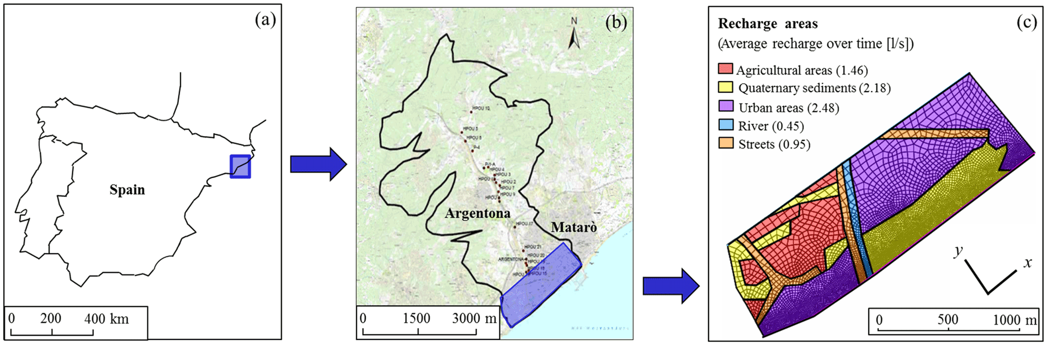
Figure 1(a) Location of the Argentona river basin. (b) Two-dimensional, constant-density model (modified from Rodriguez Fernandez, 2015). Pumping wells (brown dots) and three-dimensional model location (blue shaded area) are also depicted. (c) Planar view of the three-dimensional variable-density flow and transport model. The unstructured grid and diverse recharge areas are also shown.
Section 2 provides a general description of the field site, the mathematical model adopted to simulate flow and transport phenomena in three-dimensional heterogeneous systems and the numerical settings. Section 3 illustrates the key results of our work and Sect. 4 contains our concluding remarks.
2.1 Site description
To consider a realistic scenario that is relevant to SWI problems in highly exploited aquifers, we cast our analysis in a setting inspired from the Argentona river basin, located in the region of Maresme, in Catalonia, Spain (see Fig. 1a). This aquifer is a typical deltaic site, characterized by shallow sedimentary units and a flat topography. As such, it has a strategic value for anthropogenic (including agricultural, industrial and touristic) activities. The geological formation hosting the groundwater resource is mainly composed of a granitic Permian unit. A secondary unit of quaternary sediments is concentrated along the Argentona river.
Rodriguez Fernandez (2015) developed a conceptual and numerical model to simulate transient two-dimensional (horizontal) constant-density flow in the Argentona river basin across the area of about 35 km2 depicted in Fig. 1b. The aquifer is heavily exploited, as shown by the large number of wells included in Fig. 1b, mainly located along the Argentona river. The latter is a torrential ephemeral stream, in which water flows only after heavy rain events. On these bases, it is assumed that the only water intake to the river comes from surface runoff of both granitic and quaternary units. On the basis of transient hydraulic head measurements available at 21 observation wells (not shown in Fig. 1b) in the period 2006–2013, Rodriguez Fernandez (2015) characterized the site through a uniform permeability, whose value was estimated as kB = 1.77 × 10⁻¹¹ m2, and provided estimates of temporally and spatially variable recharge rates, according to land use or cover (see Fig. 1c).
Our numerical analysis focuses on the coastal portion of the Argentona basin (Fig. 1c). This region extends for about 2.5 km along the coast (i.e., along the full width of the basin) and up to 750 m inland from the coast. The offshore extension of the aquifer is not considered. The size of the study area has been selected on the basis of the results of preliminary simulations on larger domains, which highlighted that salt concentration values were appreciable only within a narrow (less than 400 m wide) region close to the coast. The vertical thickness of the domain ranges from 50 m along the coast up to 60 m at the inland boundary, the underlying clay sequence being considered to represent the impermeable bottom of the aquifer. SWI is simulated by means of a three-dimensional variable-density flow and solute transport model based on the well-established finite element USGS SUTRA code (Voss and Provost, 2002) over the 8-year time window 2006–2013. Details of the mathematical and numerical model are discussed in the following sections.
2.2 Flow and transport equations
Fluid flow is governed by mass conservation and Darcy's law:
where q (L T−1) is the specific discharge vector, with components qx, qy and qz, respectively, along x, y (see Fig. 1c) and z axes (z denoting the vertical direction); C (–) is solute concentration, or solute mass fraction, expressed as mass of solute per unit mass of fluid; k (L2) is the diagonal permeability tensor, with components k11 = kx, k22 = ky and k33 = kz, respectively, along directions x, y and z; ϕ (–) is aquifer porosity; ρ (M L−3) and μ (M L−1 T−1), respectively, are fluid density and dynamic viscosity; p (M L−1 T−2) is fluid pressure; g (L T−2) is gravity; SS (L−1) is the specific storage coefficient, and the superscript T denotes transpose. Equations (1) and (2) must be solved jointly with the advection–dispersion equation:
D (L2 T−1) is the dispersion tensor defined as
where Dm (L2 T−1) is the molecular diffusion coefficient, and αL and αT (L), respectively, are the longitudinal and transverse dispersivity coefficients. Closure of the system of Eqs. (1)–(4) requires a relationship between fluid properties (ρ and μ) and solute concentration C. Fluid viscosity can be assumed constant in typical SWI settings and the following model has been shown to be accurate at describing the evolution of ρ with C (Kolditz et al., 1998):
where CS is SW concentration. Table 1 lists aquifer and fluid parameters adopted.
2.3 Numerical model
The domain depicted in Fig. 1c is discretized through an unstructured three-dimensional grid formed by 101 632 hexahedral elements. The resolution of the mesh increases towards the sea, where our analysis requires the highest spatial detail. The element size along both horizontal directions x and y ranges from 10 m (in a 200 m wide region along the coast) to 60 m (close to the inland boundary). Element size along the vertical direction is 2 and 4 m, respectively, within the first 10 m from the top surface and across the remaining 40 m. These choices are consistent with constraints for numerical stability, namely ΛL≤4αL, ΛL being the distance between element sides measured along a flow line and αL=5 m. In the absence of transverse dispersivity estimates and in analogy with main findings of previous works (e.g., Cobaner et al., 2012), we set .
A sequential Gaussian simulation algorithm (Deutsch and Journel, 1998) is employed to generate unconditional log permeability fields, Y(x)=ln k(x), characterized by a given mean 〈Y〉=ln kB and variogram structure. Since no Y data are available, for the purpose of our simulations we assume that the spatial structure of Y is described by a spherical variogram, with moderate variance, i.e., , and isotropic correlation scale λ=100 m. This value is consistent with the observation that the integral scale of log conductivity and transmissivity values inferred worldwide using traditional (such as exponential and spherical) variograms tends to increase with the length scale of the sampling window at a rate of about 1∕10 (Neuman et al., 2008). The MC approach allows us to provide a probabilistic description of the SWI processes associated with space–time distributions of flux and solute concentration obtained in each random realization of the permeability field by solving the transient flow and transport Eqs. (1)–(5). Note also that λ>5Δ in our model, Δ being the largest cell size within a 200 m wide region along the coast. A model satisfying this condition has the benefit of (a) yielding a proper reconstruction of the spatial correlation structure of Y and (b) limiting the occurrence of excessive variations between values of aquifer properties across neighboring cells (Kerrou and Renard, 2010) in the region where SWI takes place.
Equations (1)–(5) are solved jointly, adopting the following boundary conditions. The lateral boundaries perpendicular to the coastline and the base of the aquifer are impervious; along the inland boundary we set a time-dependent prescribed hydraulic head, hF (with ) ranging between 1.2 and 3.5 m), and C=CF; along the coastal boundary we impose a prescribed head, hS=0 (with ), and
n being the normal vector pointing inward along the boundary; i.e., the concentration of the water entering and leaving the system across the coastal boundary is, respectively, equal to CS and C. The area of interest is characterized by five recharge zones, identified on the basis of the land use (inferred from the SIGPAC, 2005, dataset). The total recharge varies slightly in time (on a monthly basis), with mean value equal to 7.6 L s−1 (see Fig. 1c). Initial conditions are set as h=0 and C=0, as commonly assumed in the literature (e.g., Jakovovic et al., 2016) and flow and transport are simulated for an 8-year period (2006–2013) with a uniform time step Δt=1 day. Varying the initial conditions (e.g., setting, h=2.4 m, corresponding to the mean value of h set along the inland boundary), did not lead to significantly different results at the end of the simulated 8-year period, t=tw (details not shown).
A pumping well is activated at time tw and flow and transport are simulated for 8 additional months. We consider three diverse pumping schemes, reflecting realistic engineered operational settings. The borehole is located along the vertical cross-section B–B′, as shown in Fig. 2a. Scheme 1 (S1) and Scheme 2 (S2) consider the pumping well to be placed 180 m away from the shoreline, i.e., at y′ = y∕λ = 1.8, outside of the mixing zone which is in place prior to pumping in all MC realizations. In S1 (Fig. 2b) the well is screened in the upper part of the aquifer, the screen starting from 2 m below the top and extending across a total thickness of 15 m. The double-negative hydraulic barrier is a technology employed to manage (or possibly prevent) SWI. It relies on the joint use of an FW (production well) and an SW (scavenger well) pumping well. We employ this setting in S2 (Fig. 2c), which is designed by adding an additional screen in the lower part of the aquifer to S1, starting from 34 m below the ground surface and extending across a total thickness of 12 m. In S2, production and scavenger wells are located along the same borehole, complying with technical and economic requirements typically associated with field applications (Pool and Carrera, 2009; Saravanan et al., 2014; Mas-Pla et al., 2014). This scheme is also particularly appealing when applied to renewable energy resources, such as the pressure retarded osmosis, which allows conversion of the chemical energy of two fluids (FW and SW) into mechanical and electrical energy (Panyor, 2006). Scheme 3 (S3, Fig. 2d) shares the same operational design of S2, but the borehole is moved seawards, at y′ = 0.8, i.e., within the mixing zone in place before pumping. In all pumping schemes, the withdrawal rate is constant in time and uniformly distributed along the well screens, where pumping is implemented by setting a flux-type condition. We set a total withdrawal rate Q = 5 L s−1 at the upper well screen in S1, S2 and S3; an additional extraction at the same rate Q is imposed along the lower screen in S2 and S3. During the pumping period, transport is simulated using a time step Δt = 30 min for the first month and with increasing Δt progressively up to a maximum value Δt = 120 min for the remaining 7 months, as the system showed progressively smoother variations while approaching steady state. In Sect. 3 all schemes are compared against a benchmark case, Scheme 0 (S0), where no pumping wells are active.
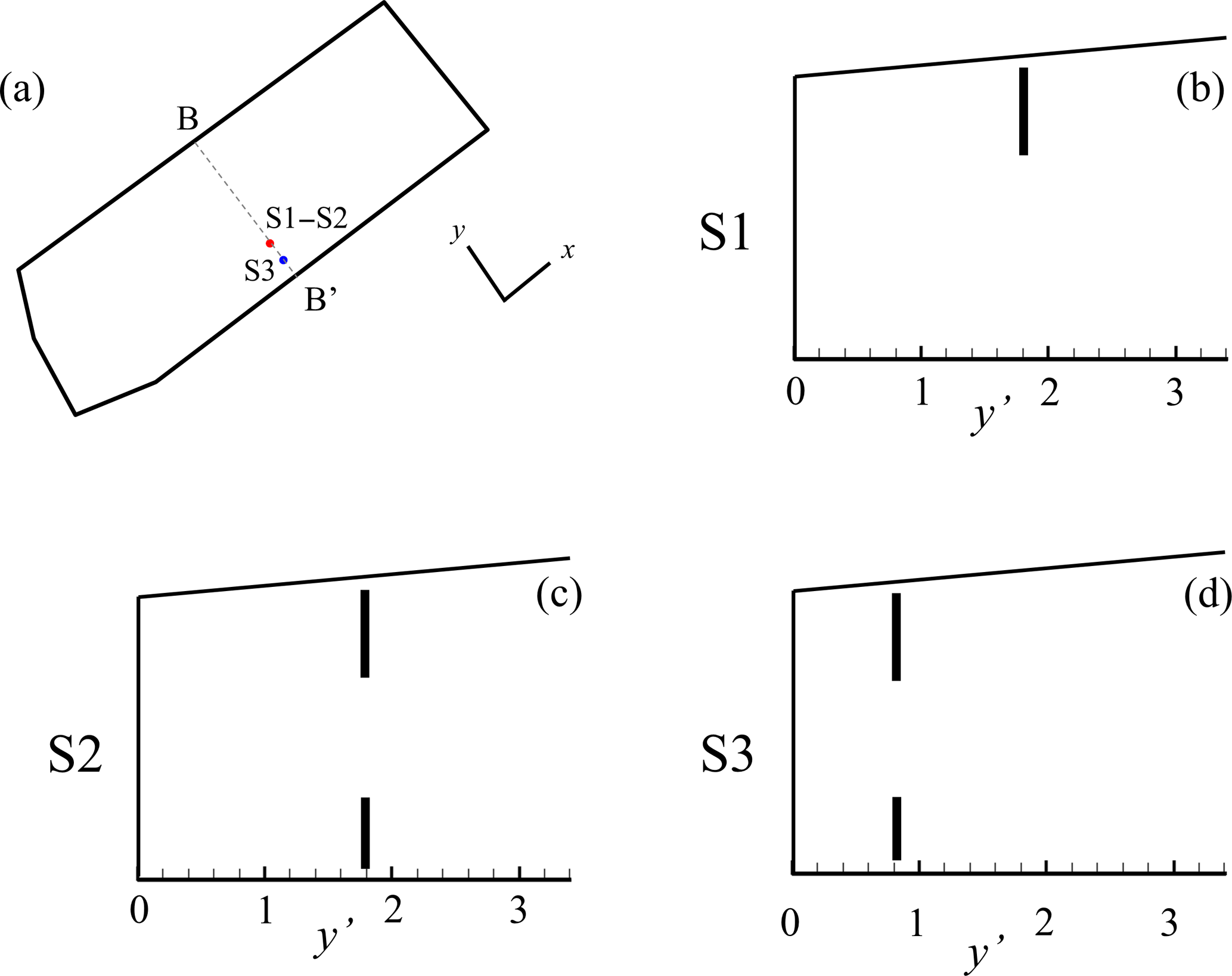
Figure 2(a) Planar view of the location of the boreholes. Vertical cross section B–B′ and well-screen location for scheme (b) S1, (c) S2 and (d) S3.
2.4 Local and global SWI metrics
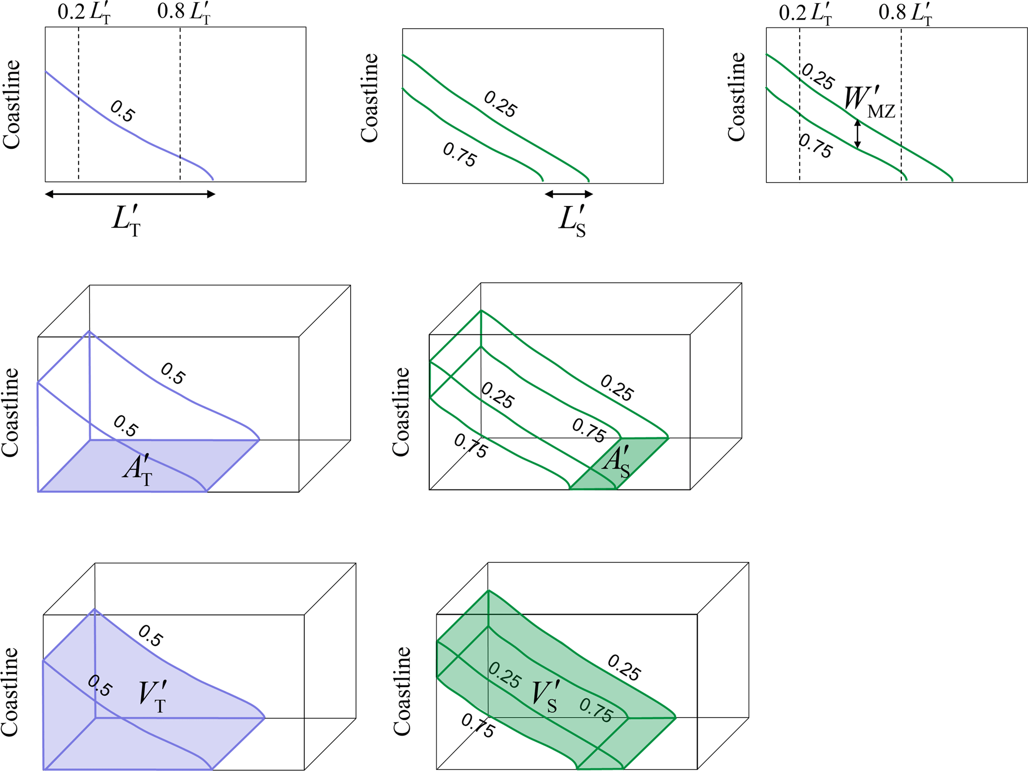
To provide a comprehensive characterization of SWI phenomena across the whole three-dimensional domain, we quantify the extent of the SW wedge and of the associated mixing zone on the basis of seven metrics, as illustrated in Fig. 3.
For each MC realization and along each vertical cross-section perpendicular to the coast, we evaluate (i) toe penetration, , measured as the distance from the coast of the iso-concentration curve C∕CS = 0.5 at the bottom of the aquifer; (ii) solute spreading at the toe, , evaluated as the separation distance along the direction perpendicular to the coast (y axis in Fig. 1c) between the iso-concentration curves C∕CS = 0.25 and C∕CS = 0.75 at the bottom of the aquifer; (iii) mean width of the mixing zone, , i.e., the spatially averaged vertical distance between iso-concentration curves C∕CS = 0.25 and C∕CS = 0.75 within the region ≤ y′ ≤ . All quantities , and are dimensionless, corresponding to distances rescaled by λ, the correlation scale of Y. We also analyze the (dimensionless) areal extent of SW penetration and solute spreading at the bottom of the aquifer by evaluating (iv) and (v) , as obtained by integrating and along the coastline. Finally, we quantify SWI across the whole thickness of the aquifer by evaluating the dimensionless volumes enclosed between (vi) the sea boundary and the iso-concentration surface C∕CS = 0.5, here termed , and (vii) the isosurfaces C∕CS = 0.25 and C∕CS = 0.75, here termed . First- and second-order statistical moments of each of these metrics are evaluated within the adopted MC framework. With the settings employed here, a flow and transport simulation on a single system realization is associated with a computational cost of about 12 h (on an Intel Core™ i7-6900K CPU@ 3.20 GHz processor). Results illustrated in the following sections are based on a suite of 400 MC simulations (i.e., 100 MC simulation for each scenario, S0–S3). Details concerning the analysis of convergence of the first and second statistical moments of the metrics here introduced are provided in Appendix A.
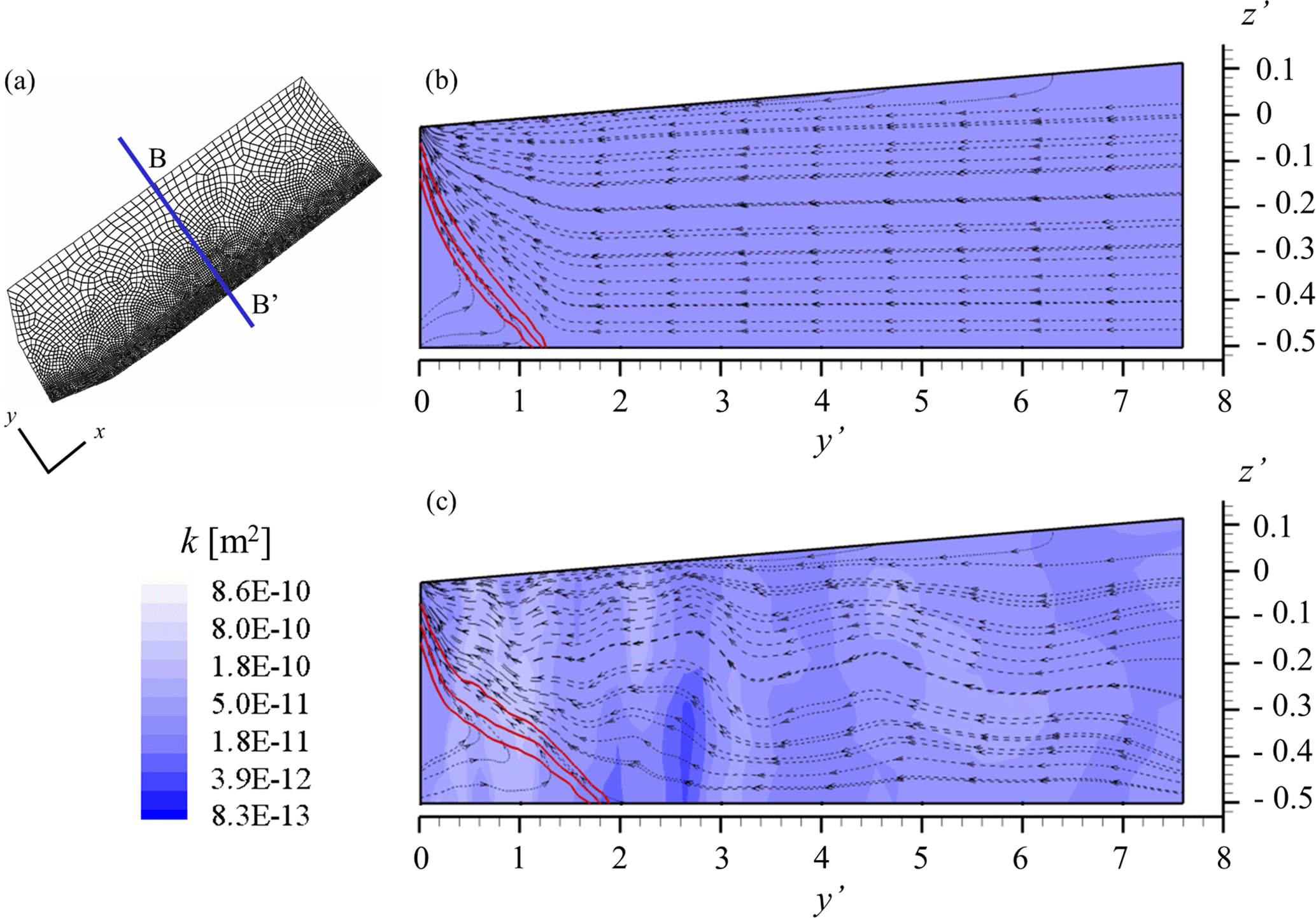
Figure 4Permeability distribution (color contour plots), streamlines (black dashed curves) and iso-concentration curves C∕CS = 0.25, 0.5 and 0.75 (solid red curves) along the cross-section B–B′ evaluated at t=tw within (b) the equivalent homogeneous aquifer and (c) one random realization of k. Vertical exaggeration = 5.
3.1 Effects of three-dimensional heterogeneity on SWI
The effects of heterogeneity on SWI are inferred by comparing the results of our MC simulations against those obtained for an equivalent homogeneous aquifer, characterized by an effective permeability, kef. The latter is here evaluated as m2 (Ababou, 1996). A first clear effect of heterogeneity is noted on the structure of the three-dimensional flow field. This is elucidated in Fig. 4, where we depict the permeability color map and streamlines (dashed curves) obtained at the end of the 8-year simulation period along the vertical cross-section B–B′ perpendicular to the coastline. Note that henceforth, results are depicted in terms of dimensionless spatial coordinates, y′ = y∕λ and z′ = z∕λ. Flow within the equivalent homogeneous aquifer (Fig. 4b) is essentially horizontal at locations far from the zone where SWI phenomena occur. Otherwise, the vertical flux component, qz, is non-negligible throughout the whole domain for the heterogeneous system (Fig. 4c) and streamlines tend to focus towards regions characterized by large permeability values. Figure 4 also depicts iso-concentration curves C∕CS = 0.25, 0.5 and 0.75 within the transition zone (red curves). It can be noted that iso-concentration profiles tend to be sub-parallel to streamlines directed towards the seaside boundary. In the homogeneous domain the slope of these curves varies mildly and in a gradual manner from the top to the bottom of the aquifer. Their slope in the heterogeneous domain is irregular and markedly influenced by the spatial arrangement of permeability. In other words, the way streamlines are refracted at the boundary between two blocks of contrasting permeability drives the local pattern of concentration contour lines. As a consequence, iso-concentration curves tend to become sub-vertical when solute is transitioning from regions characterized by high k values to zones associated with moderate to small k, a sub-horizontal pattern being observed when transitioning from low to high k values.
Figure 5 depicts isolines C∕CS = 0.5 at the bottom of the aquifer (Fig. 5a) and along three vertical cross-sections, selected to exemplify the general pattern observed in the system (Fig. 5b–d), evaluated for (i) the 100 heterogeneous realizations analyzed (dotted blue curves), (ii) the equivalent homogeneous system (denoted as Hom; solid red curve) and (iii) the configuration obtained by averaging the concentration fields across all MC heterogeneous realizations (denoted as Ens; solid blue curve). These results suggest that iso-concentration curves exhibit considerably large spatial variations within a single realization. Comparison of the results obtained for Ens and Hom reveals that the mean wedge penetration at the bottom layer is slightly overestimated by the solution computed within the equivalent homogeneous system. Otherwise, along the coastal vertical boundary, the extent of the area with (mean) relative concentration larger than 0.5 is generally underestimated by Hom. These outcomes (hereafter called rotation effects) are consistent with previous literature findings associated with (a) deterministic models (Abarca et al., 2007) or (b) stochastic analyses performed under ergodicity assumptions (Kerrou and Renard, 2010, and Pool et al., 2015). Abarca et al. (2007) showed that a similar effect can be observed in a homogenous domain when considering increasing values of the dispersion coefficient. Kerrou and Renard (2010) and Pool et al. (2015) noted that the strength of the rotation effect increases with the variance of the log permeability field.
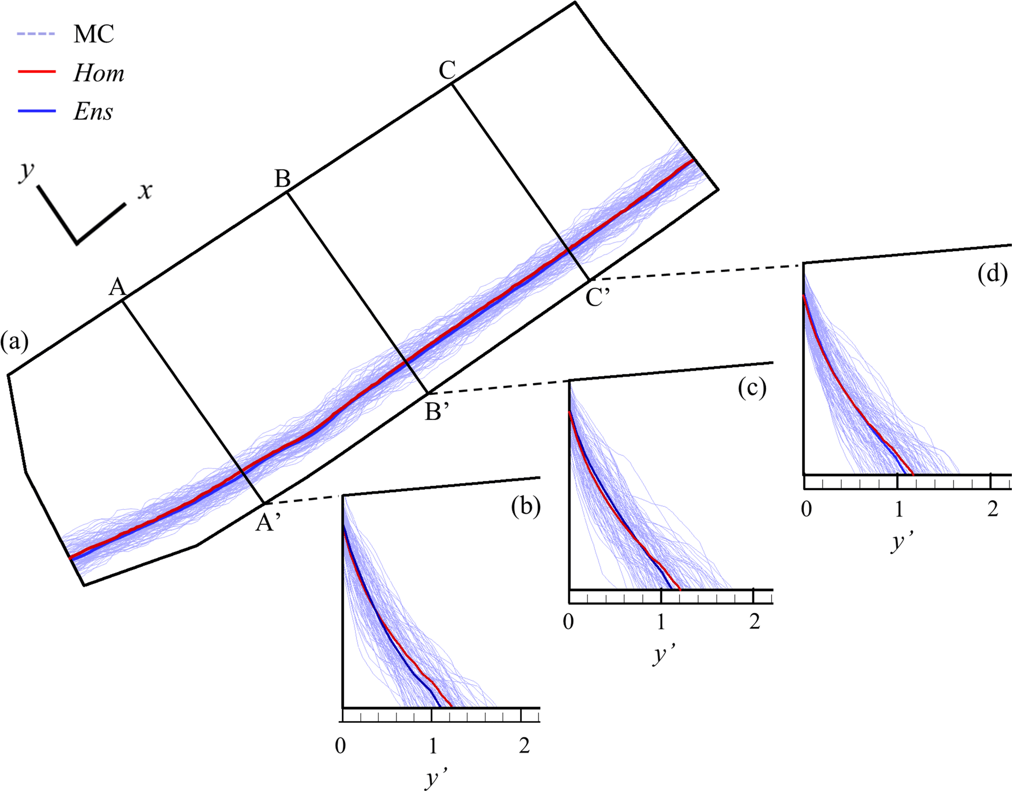
Figure 5MC-based (dotted blue curves) iso-concentration lines C∕CS = 0.5 at t=tw along (a) the bottom of the aquifer and (b–d) three vertical cross-sections perpendicular to the coast. The ensemble-average concentration curves (solid blue curve) and the results obtained within the equivalent homogeneous system (solid red curve) are also reported. Vertical exaggeration = 5.
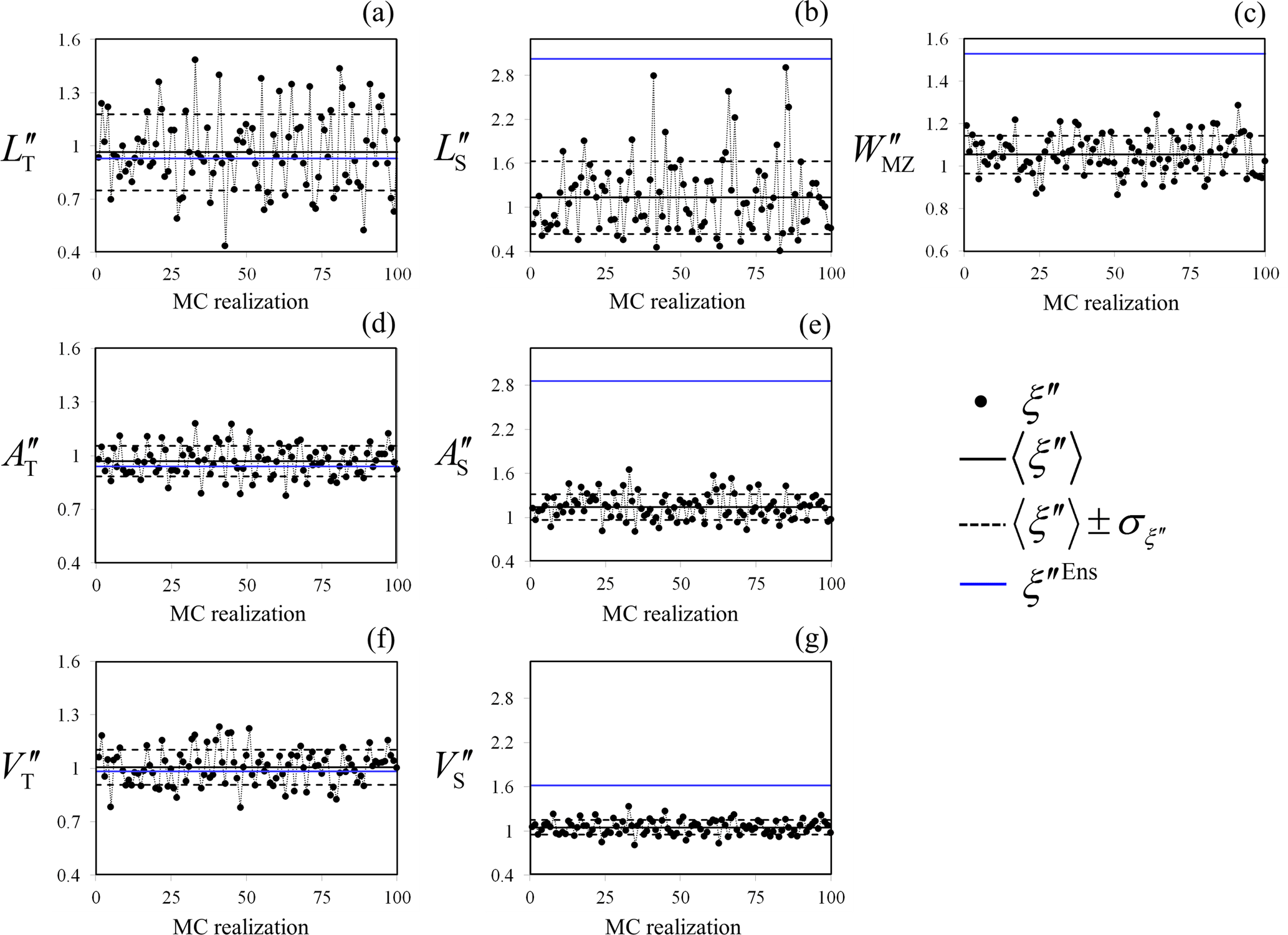
Figure 6Metrics evaluated at t=tw within each MC heterogeneous realization (dots) and on the basis of the ensemble-average concentration field (blue line). Ensemble mean metrics (solid black line) and confidence intervals of width equal to ± 1 standard deviation of ξ′′ about their mean (dashed black lines) are also depicted. Metrics in (a–c) are computed along the vertical cross-section B–B′.
In the following, we analyze values of , ξ′ representing a given SWI metric (as listed in Sect. 2.4) and ξ′Hom being the corresponding metric obtained on the equivalent homogeneous system. Figure 6 depicts the range of variability of ξ′′ across the set of MC realizations (symbols). Each plot is complemented by the depiction of (i) the (ensemble) average of ξ′′, as evaluated through all MC realizations, 〈ξ′′〉 (black solid line); (ii) the confidence intervals, (black dashed lines), being the standard deviation of ξ′′; (iii) ξ′′Ens, evaluated on the basis of the ensemble-average concentration field (blue line). Inspection of Fig. 6a–c complements the qualitative analysis of Fig. 5 and suggests that heterogeneity causes (on average) a slight reduction of the toe penetration, and being slightly less than 1, and an enlargement of the mixing zone, and being larger than 1. The results of Fig. 6a–c also emphasize that, while calculated from the ensemble-average concentration distributions is virtually indistinguishable from , and markedly overestimate and , respectively, as they visibly lie outside of the corresponding confidence intervals of width . Note that even as Fig. 6a–c have been computed along cross-section B–B′, qualitatively similar results have been obtained along all vertical cross-sections, as also suggested by the behavior of the dimensionless areal extent of toe penetration, (Fig. 6d), and solute spreading, (Fig. 6e), as well as of the dimensionless volumes and (Fig. 6f–g). Overall, the results in Fig. 6 clearly indicate that the ensemble-average concentration field can provide accurate estimates of the average wedge penetration while rendering biased estimates of quantities characterizing mixing. Our findings are consistent with previous studies (e.g., Dentz and Carrera, 2005; Pool et al., 2015) in showing that an analysis relying on the ensemble concentration field tends to overestimate significantly the degree of mixing and spreading of the solute because it combines the uncertainty associated with sample-to-sample variations of (a) the solute center of mass and (b) the actual spreading. Our results also highlight that the extent of this overestimation decreases whenever integral rather than local quantities are considered: in Fig. 6g is indeed about half of and .
3.2 Effects of pumping on SWI in three-dimensional heterogeneous media
Here, we investigate SWI phenomena in heterogeneous systems when a pumping scheme is activated as described in Sect. 2.3. Figure 7 collects contour maps of relative concentration C∕CS obtained for all schemes along cross-section B–B′ at the end of the 8-month pumping period, with reference to (i) Hom (the equivalent homogeneous system, left column) and (ii) Ens (the ensemble-average concentration field, right column). Contour lines C∕CS = 0.25, 0.50 and 0.75 are also highlighted. Extracting FW according to the engineered solution S1 (Fig. 7c–d) results in a slight landward displacement of the SWI wedge and in an enlargement of the transition zone, as compared to S0 (Fig. 7a–b), where no pumping is activated. This behavior can be observed in the homogeneous as well as (on average) in the heterogeneous settings, and is related to the general decrease of the piezometric head within the inland side caused by pumping which, in turn, favors SWI. One can also note that the partially penetrating well induces non-horizontal flow (in the proximity of the well) thus enhancing mixing along the vertical direction. Wedge penetration and solute spreading are further enlarged in S2 (see Fig. 7e–f), where the total extracted volume is increased with respect to S1 through an additional pumping rate at the bottom of the aquifer. However, when the pumping well is operating within the transition zone (S3, Fig. 7g–h) the SW wedge tends to recede, approaching the pumping well location. In this case, the lower screen acts as a barrier limiting the extent of the SWI at the bottom of the aquifer.
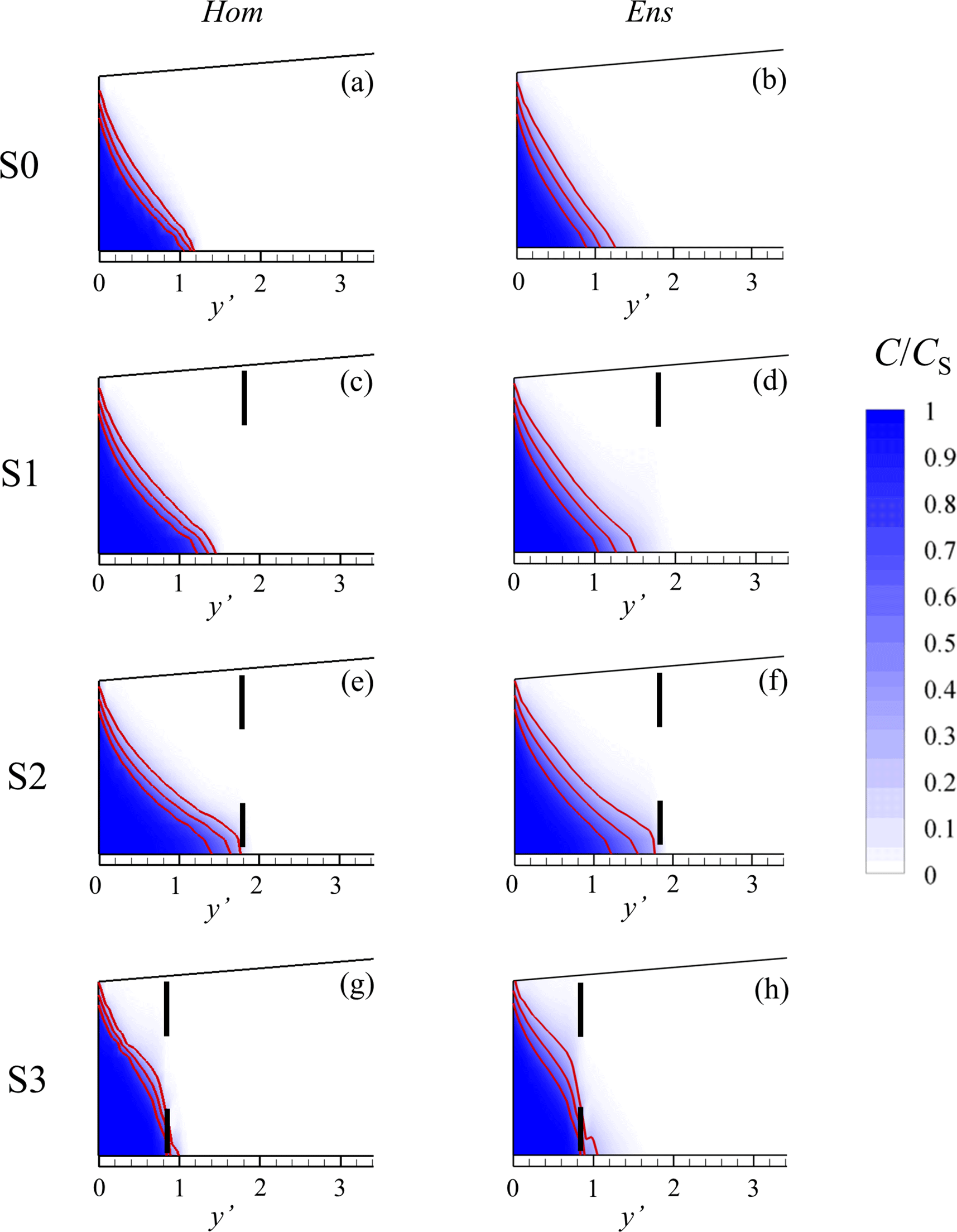
Figure 7Concentration distribution (color contour plots) and iso-concentration lines C∕CS = 0.25, 0.5 and 0.75 (solid red curves) along the cross-section B–B′ shown in Fig. 2a evaluated at the end of the pumping period within the equivalent homogeneous aquifer (left column) and the ensemble-average concentration field (right column). Black vertical lines represent the location of the well screens. Vertical exaggeration = 5.
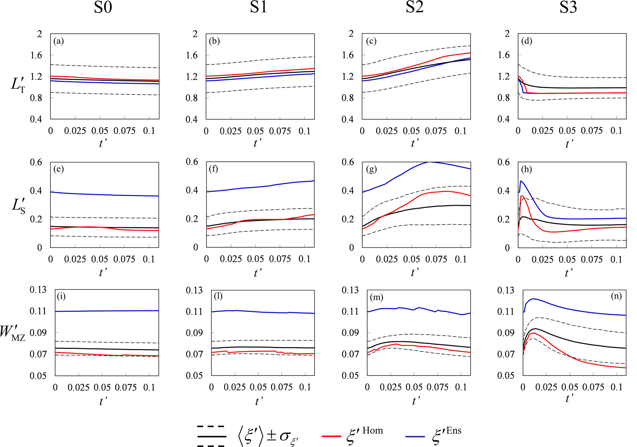
Figure 8Temporal evolution of , and evaluated along the vertical cross-section B–B′ shown in Fig. 2a during the pumping period, for all pumping schemes within the equivalent homogeneous domain (red lines) and the ensemble-average concentration field (blue lines). MC-based mean values of ξ′ (black lines) and confidence intervals of width equal to ± 1 standard deviation of ξ′ about their mean are also depicted.
The combined effects of groundwater withdrawal and stochastic heterogeneity on SWI are investigated quantitatively through the analysis of the temporal evolution of the seven metrics introduced in Sect. 2.4.
Figure 8 illustrates mean values of ξ′ (with , and ) computed for all pumping schemes considered across the collection of all heterogeneous realizations (black line) along the vertical cross-section B–B′ versus dimensionless time . Confidence intervals are also depicted (dashed lines). As additional terms of comparison, Fig. 8 also includes ξ′Hom (red line) and ξ′Ens (blue line), respectively, evaluated in the equivalent homogeneous domain and in the ensemble-average concentration field. Figure 8 shows that the toe penetration, , and the solute spreading, as quantified by and , do not vary significantly with time in the absence of pumping (S0) because stationary boundary conditions are imposed for . Pumping schemes S1 and S2 cause the progressive inland displacement of the toe, together with an overall increase of spreading at the bottom of the aquifer. This phenomenon is more severe in S2, where SW and FW are simultaneously extracted. On the other hand, the vertical width of the mixing zone, e.g., , is not significantly affected by the pumping within schemes S1–S2. Configuration S3, in which the pumping well is located within the mixing zone, leads to the most pronounced changes in the shape and position of the SW wedge. The toe penetration first decreases rapidly in time and then stabilizes around the well location. Quantities and show an early time increase, suggesting that a rapid displacement of the wedge enhances mixing and spreading. As the toe stabilizes over time, both and decrease, reaching values equal to (or slightly less than) those detected in the absence of pumping. Consistent with the observations of Sect. 3.1, Fig. 8 supports the findings that (i) an equivalent homogeneous domain is typically characterized by the largest toe penetration and the smallest vertical width of the mixing zone, the only exception being observed in S3 at late times, when ; (ii) basing the characterization of the mixing zone on ensemble-average concentrations enhances the actual effects of heterogeneity and yields overestimated mixing zone widths. Figure 8 also highlights that the extent of the confidence interval associated with toe penetration is approximately constant in time and does not depend significantly on the analyzed flow configuration. Otherwise, the confidence intervals associated with our mixing zone metrics depend on the pumping scenario and tend to increase with time if FW and SW are simultaneously extracted, especially in S2.
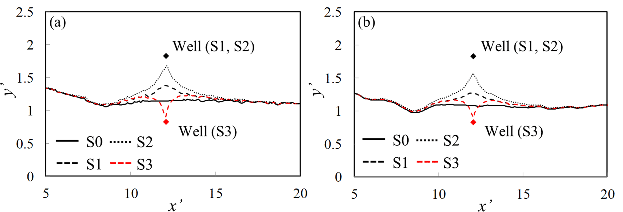
Figure 9Isolines C∕CS = 0.5 at the end of the pumping period along the bottom of the aquifer for the four schemes S0–S3 evaluated (a) within the equivalent homogeneous domain and (b) from the ensemble-average concentration field.
The fully three-dimensional nature of the analyzed problem is exemplified in Fig. 9, where we depict isolines C∕CS = 0.5 along the bottom of the aquifer at the end of the pumping period for the equivalent homogeneous system (Fig. 9a) and as a result of ensemble averaging across the collection of heterogeneous fields (Fig. 9b). The spatial pattern of iso-concentration contours associated with pumping schemes S1–S3 departs from the corresponding results associated with S0 within a range extending for about 10λ around the well, along the direction parallel to the coastline.

Figure 10Temporal evolution of , where , , evaluated for all pumping schemes within the equivalent homogeneous domain (red lines) and the ensemble-average concentration field (blue lines). MC-based mean values of ξ∗ (black lines) and confidence intervals of width equal to ± 1 standard deviation of ξ∗ about their mean are also depicted.
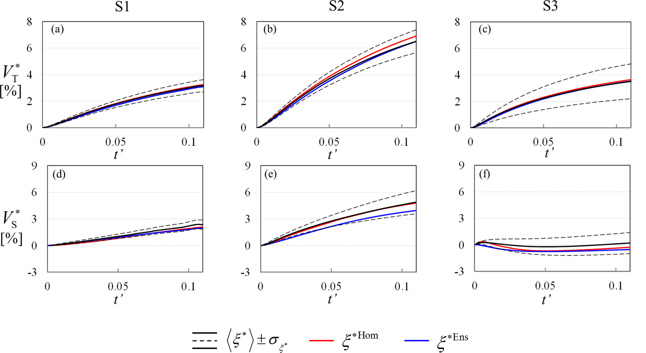
Figure 11Temporal evolution of , where , , evaluated for all pumping schemes within the equivalent homogeneous domain (red lines) and the ensemble-average concentration field (blue lines). MC-based mean values of ξ∗ (black lines) and confidence intervals of width equal to ± 1 standard deviation of ξ∗ about their mean are also depicted.
We quantify the global effect of pumping on the three-dimensional SW wedge by evaluating, for each pumping scenario and each MC realization, the temporal evolution of , i.e., the relative percentage variation of areal extent, , and volumetric extent, , of wedge penetration and mixing zone with respect to their counterparts computed in the absence of pumping . Figure 10 shows that the penetration area, , and the solute spreading, as quantified through , at the bottom of the aquifer tend to increase with pumping time. Corresponding results for and are depicted in Fig. 11. The scenario where these quantities are most affected by pumping is S2, where the FW and SW pumping wells are located outside the transition zone (in place prior to pumping). Placing both wells within the transition zone prior to pumping yields a significant decrease of the effect of pumping on both areal and volumetric metrics. We further note that the mean penetration area and volume can be accurately determined by the solution obtained within the equivalent homogeneous domain and is associated with a relatively small uncertainty, as quantified by the confidence intervals. Heterogeneity effects are clearly visible on spreading along the bottom of the aquifer. Figure 10d–f highlight that and are not accurate approximations of . Spreading uncertainty, as quantified by , is significantly larger than , especially in pumping scenario S2. On the other hand, the spreading of the SWI volume, as quantified by (Fig. 11d–f), can be accurately estimated by the homogeneous equivalent system, as well as by the ensemble mean concentration field, and it is characterized by a relatively low uncertainty.
Our analyses document that for a stochastically heterogeneous aquifer an operational scheme of the kind engineered in S3 (i) is particularly efficient for the reduction of SWI maximum penetration (localized at the bottom of the aquifer) and (ii) is advantageous in controlling the extent of the volume of the SW wedge, as compared to the double-negative barrier implemented in S2. However, this withdrawal system may lead to the salinization of the FW extracted from the upper screen due to upconing effects. This aspect is further analyzed in Fig. 12 where the temporal evolution of CT∕CS is depicted, CT being the salt concentration associated with the total mass of fluid extracted by the upper screen (production well) in S3. Results for the equivalent homogeneous system (red curve), each of the heterogeneous MC realizations (grey dashed curves) and the ensuing ensemble-average concentration 〈CT〉∕CS (blue curve) are depicted. Vertical bars represent the 95 % confidence interval around the ensemble mean, evaluated as . Here is the standard deviation of CT∕CS and n=100 is the number of MC realizations forming the collection of samples. The width of these confidence intervals can serve as a metric to quantify the order of magnitude of the uncertainty associated with the estimated mean. The equivalent homogeneous system significantly underestimates the ratio 〈CT〉∕CS. Moreover, Fig. 12 highlights the marked variability of the results across the MC space. As such, it reinforces the conclusion that the mean value 〈CT〉 is an intrinsically weak indicator of the actual salt concentration at the producing well.
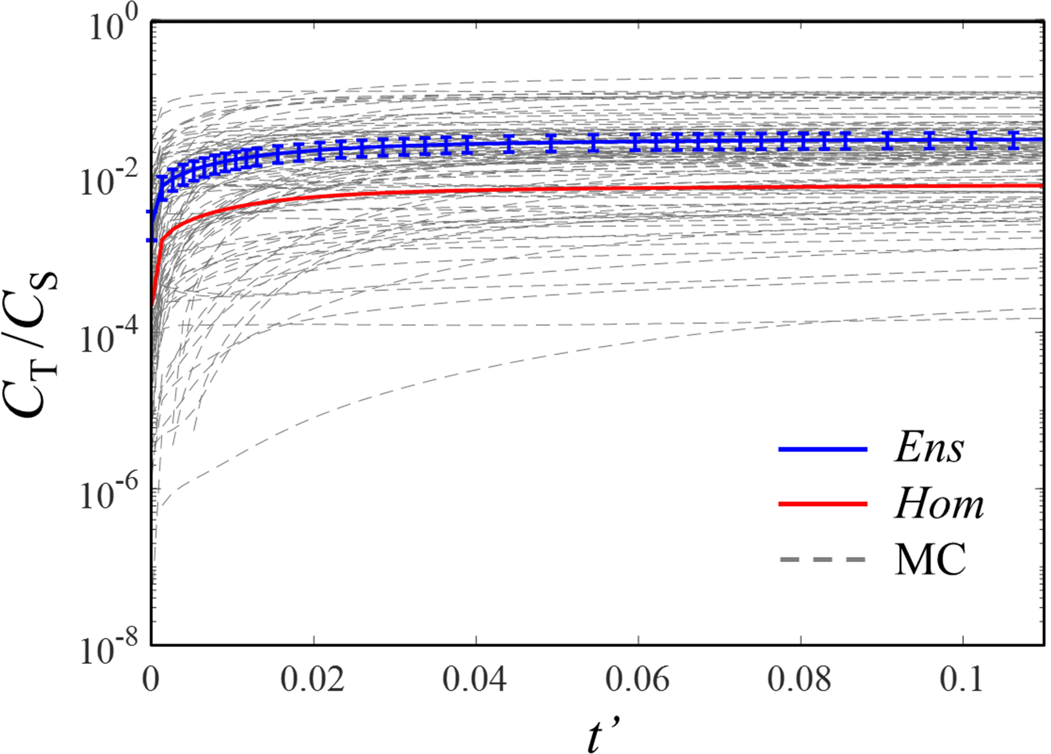
Figure 12Temporal evolution of CT∕CS for pumping scheme S3 within the equivalent homogeneous system (red curve) and for each heterogeneous realization (gray dashed curves). The ensemble-average (blue curve) dimensionless concentration and its 95 % confidence interval are also depicted.
We investigate quantitatively the role of stochastic heterogeneity and groundwater withdrawal on seawater intrusion (SWI) in a randomly heterogeneous coastal aquifer through a suite of numerical Monte Carlo (MC) simulations of transient variable-density flow and transport in a three-dimensional domain. Our work attempts to include the effects of random heterogeneity of permeability and groundwater withdrawal within a realistic and relevant scenario. For this purpose, the numerical model has been tailored to the general hydrogeological setting of a coastal aquifer, i.e., the Argentona river basin (Spain), a region which is plagued by SWI. To account for the inherent uncertainty associated with aquifer hydrogeological properties, we conceptualize our target system as a heterogeneous medium whose permeability is a random function of space. The SWI phenomenon is studied through the analysis of (a) the general pattern of iso-concentration curves and (b) a set of seven dimensionless metrics describing the toe penetration and the extent of the mixing or transition zone. We compare results obtained across a collection of n=100 MC realizations and for an equivalent homogeneous system. Our work leads to the following major conclusions.
Heterogeneity of the system affects the SW wedge along all directions both in the presence and absence of pumping. On average, our heterogeneous system is characterized by toe penetration and extent of the mixing zone that are, respectively, smaller and larger than their counterparts computed in the equivalent homogeneous system.
Ensemble (i.e., across the MC realizations) mean values of linear, , areal, , and volumetric, , metrics representing 50 % of SWI penetration virtually coincide with their counterparts evaluated in the ensemble-average concentration field.
Ensemble mean values of linear, and , and areal, , metrics representing the mixing and spreading of SWI penetration are markedly overestimated by their counterparts evaluated on the basis of the ensemble-average concentration field. Therefore, average concentration fields, typically estimated through interpolation of available concentration data, cannot be employed to provide reliable estimates of solute spreading and mixing.
All of the tested pumping schemes lead to an increased SW wedge volume compared to the scenario where pumping is absent. The key aspect controlling the effects of groundwater withdrawal on SWI is the position of the wellbore with respect to the location of the saltwater wedge in place prior to pumping. The toe penetration decreases or increases depending on whether the well is initially (i.e., before pumping) located within or outside the seawater intruded region, respectively. The water withdrawal scheme that is most efficient for the reduction of the maximum inland penetration of the seawater toe is the one according to which freshwater and saltwater are, respectively, extracted from the top and the bottom of the same borehole, initially located within the SW wedge. This result suggests the potential effectiveness of the so-called “negative barriers” in limiting intrusion, even when considering the uncertainty effects stemming from our incomplete knowledge of permeability spatial distributions.
Salt concentration, CT, of water pumped from the producing well is strongly affected by permeability heterogeneity. Our MC simulations document that CT can vary by more than 2 orders of magnitude amongst individual realizations, even in the moderately heterogeneous aquifer considered in this study. As such, relying solely on values of CT obtained through an effective homogeneous system or on the ensemble-average estimates 〈CT〉 does not yield reliable quantification of the actual salt concentration at the producing well.
Future development of our work includes the analysis of the influence of the degree of heterogeneity and of the functional format of the covariance structure of the permeability field on SWI, also in the presence of multiple pumping wells.
All data used in the paper will be retained by the authors for at least 5 years after publication and will be available to the readers upon request.
Here, we assess the stability of the MC-based first- and second-order (statistical) moments associated with the metrics introduced in Sect. 2.4. Figures A1 and A2, respectively, depict the sample mean, 〈ξ′′〉, and standard deviation, σ(ξ′′), of all metrics evaluated at the end of the 8-year period versus the number of MC simulations, n. The estimated 95 % confidence intervals, computed according to Eqs. (3) and (8)

Figure A1Sample mean of the seven dimensionless metrics at t=tw and associated 95 % confidence intervals versus ensemble size, n.
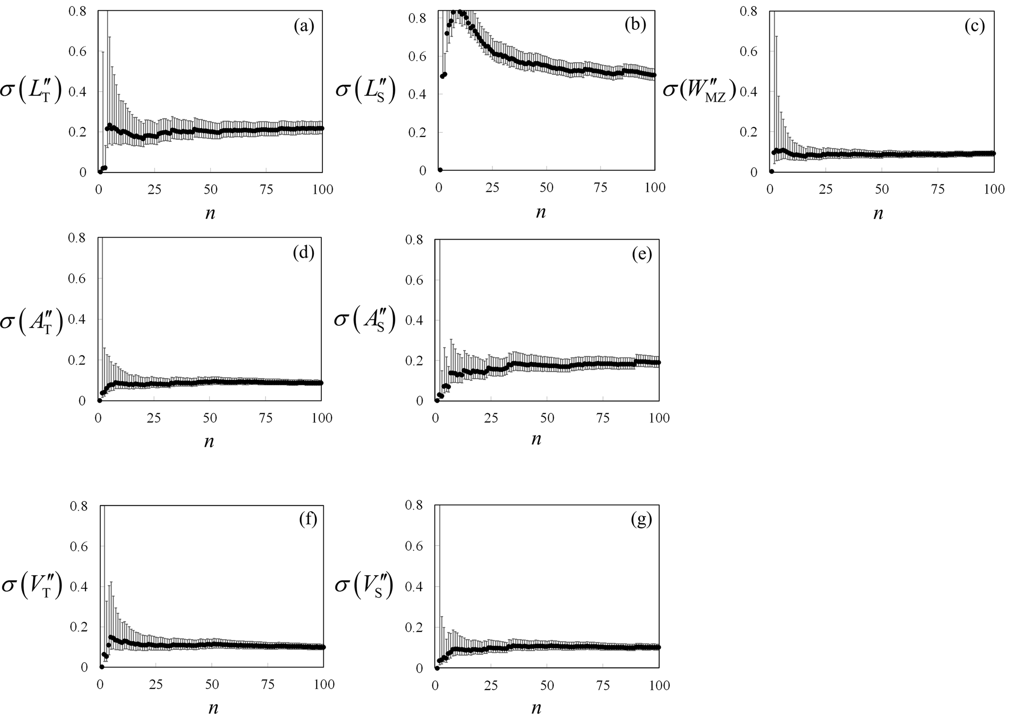
Figure A2Sample standard deviation of the seven dimensionless metrics at t=tw and associated 95 % confidence intervals versus ensemble size, n.
of Ballio and Guadagnini (2004), are also depicted. Figures A1 and A2 show that the oscillations displayed by the quantities of interest are in general limited and do not hamper the strength of the main message of our work. As expected, moments of integral quantities (i.e., , , , , ) tend to stabilize faster than their counterparts evaluated for local quantities ( and ).
The authors declare that they have no conflict of interest.
The authors would like to thank the EU and MIUR for funding,
in the frame of the collaborative international consortium (WE-NEED)
financed under the ERA-NET WaterWorks2014 Cofunded Call.
This ERA-NET is an integral part of the 2015 Joint Activities
developed by the Water Challenges for a Changing World Joint Programme Initiative (Water JPI).
We are grateful to Albert Folch, Xavier Sanchez-Vila and
Laura del Val Alonso of the Universitat Politècnica de Catalunya and
Jesus Carrera of the Spanish Council for Scientific Research for sharing data
on the hydrogeological characterization of the Argentona site with
us.
Edited by: Bill X. Hu
Reviewed by: Damiano Pasetto and two anonymous referees
Ababou, R.: Random porous media flow on large 3D grids: numerics, performance and application to homogeneization, in: Environmental studies, mathematical, computational & statistical analysis, edited by: Wheeler, M. F., Springer, New York, 1–25, 1996.
Abarca, E., Carrera, J., Sánchez-Vila, X., and Dentz, M.: Anisotropic dispersive Henry problem, Adv. Water Resour., 30, 913–926, https://doi.org/10.1016/j.advwatres.2006.08.005, 2007.
Ackerer, P. and Younes, A.: Efficient approximations for the simulation of density driven flow in porous media, Adv. Water Resour., 31, 15–27, https://doi.org/10.1016/j.advwatres.2007.06.001, 2008.
Ackerer, P., Younes, A., and Mancip, M.: A new coupling algorithm for density-driven flow in porous media, Geophys. Res. Lett., 31, L12506, https://doi.org/10.1029/2004GL019496, 2004.
Albets-Chico, X. and Kassinos, S.: A consistent velocity approximation for variable-density flow and transport in porous media, J. Hydrol., 507, 33–51, https://doi.org/10.1016/j.jhydrol.2013.10.009, 2013.
Ataie-Ashtiani, B., Volker, R. E., and Lockington, D. A.: Tidal effects on sea water intrusion in unconfined aquifers, J. Hydrol., 216, 17–31, https://doi.org/10.1016/S0022-1694(98)00275-3, 1999.
Bakker, M.: Analytic solutions for interface flow in combined confined and semi-confined, coastal aquifers, Adv. Water Resour., 29, 417–425, https://doi.org/10.1016/j.advwatres.2005.05.009, 2006.
Ballio, F. and Guadagnini, A.: Convergence assessment of numerical Monte Carlo simulations in groundwater hydrology, Water Resour. Res., 40, W04603, https://doi.org/10.1029/2003WR002876, 2004.
Bolster, D. T., Tartakovsky, D. M., and Dentz, M.: Analytical models of contaminant transport in coastal aquifers, Adv. Water Resour., 30, 1962–1972, https://doi.org/10.1016/j.advwatres.2007.03.007, 2007.
Bruggeman, G. A.: Analytical Solutions of Geohydrological Problems, Developments in Water Science, 46, Elsevier Science, Amsterdam, 956 pp., 1999.
Cheng, A. H.-D., Halhal, D., Naji, A., and Ouazar, D.: Pumping optimization in saltwater-intruded coastal aquifers, Water Resour. Res., 36, 2155–2165, https://doi.org/10.1029/2000WR900149, 2000.
Cobaner, M., Yurtal, R., Dogan, A., and Motz, L. H.: Three dimensional simulation of seawater intrusion in coastal aquifers: A case study in the Goksu Deltaic Plain, J. Hydrol., 464–465, 262–280, https://doi.org/10.1016/j.jhydrol.2012.07.022, 2012.
Custodio, E.: Coastal aquifers of Europe: an overview, Hydrogeol. J., 18, 269–280, https://doi.org/10.1007/s10040-009-0496-1, 2010.
Dagan, G. and Zeitoun, D. G.: Seawater-freshwater interface in a stratified aquifer of random permeability distribution, J. Contam. Hydrol., 29, 185–203, https://doi.org/10.1016/S0169-7722(97)00013-2, 1998.
Dausman, A. and Langevin, C. D.: Movement of the Saltwater Interface in the Surficial Aquifer System in Response to Hydrologic Stresses and Water-Management Practices, Broward County, Florida, U.S. Geological Survey Scientific Investigations, Report 2004-5256, 73 pp., 2005.
Dentz, M. and Carrera, J.: Effective solute transport in temporally fluctuating flow through heterogeneous media, Water Resour. Res., 41, W08414, https://doi.org/10.1029/2004WR003571, 2005.
Dentz, M., Tartakovsky, D. M., Abarca, E., Guadagnini, A., Sanchez-Vila, X., and Carrera, J.: Variable density flow in porous media, J. Fluid Mech., 561, 209–235, https://doi.org/10.1017/S0022112006000668, 2006.
Deutsch, C. V. and Journel, A. G.: GSLIB: Geostatistical software library and user's guide, Oxford University Press, Oxford, UK, 348 pp., 1998.
Fahs, M., Younes, A., and Mara, T. A.: A new benchmark semi-analytical solution for density-driven flow in porous media, Adv. Water Resour., 70, 24–35, https://doi.org/10.1016/j.advwatres.2014.04.013, 2014.
Gingerich, S. B. and Voss, C. I.: Three-dimensional variable-density flow simulation of a coastal aquifer in southern Oahu, Hawaii, USA, Hydrogeol. J., 13, 436–450, https://doi.org/10.1007/s10040-004-0371-z, 2005.
Henry, H. R.: Effects of dispersion on salt encroachment in coastal aquifers, US Geological Survey Water-Supply Paper 1613-C, C71–C84, 1964.
Jakovovic, D., Werner, A. D., de Louw, P. G. B., Post, V. E. A., and Morgan, L. K.: Saltwater upconing zone of influence, Adv. Water Resour., 94, 75–86, https://doi.org/10.1016/j.advwatres.2016.05.003, 2016.
Kerrou, J. and Renard, P.: A numerical analysis of dimensionality and heterogeneity effects on advective dispersive seawater intrusion processes, Hydrogeol. J., 18, 55–72, https://doi.org/10.1007/s10040-009-0533-0, 2010.
Kerrou, J., Renard, P., Cornaton, F., and Perrochet, P.: Stochastic forecasts of seawater intrusion towards sustainable groundwater management: application to the Korba aquifer (Tunisia), Hydrogeol. J., 21, 425–440, https://doi.org/10.1007/s10040-012-0911-x, 2013.
Ketabchi, H., Mahmoodzadeh, D., Ataie-Ashtiani, B., and Simmons, C. T.: Sea-level rise impacts on seawater intrusion in coastal aquifers: Review and integration, J. Hydrol., 535, 235–255, https://doi.org/10.1016/j.jhydrol.2016.01.083, 2016.
Kolditz, O., Ratke, R., Diersch, H. J. G., and Zielke, W.: Coupled groundwater flow and transport: 1. Verification of variable density flow and transport models, Adv. Water Resour., 21, 27–46, https://doi.org/10.1016/S0309-1708(96)00034-6, 1998.
Lecca, G. and Cau, P.: Using a Monte Carlo approach to evaluate seawater intrusion in the Oristano coastal aquifer: A case study from the AQUAGRID collaborative computing platform, Phys. Chem. Earth, 34, 654–661, https://doi.org/10.1016/j.pce.2009.03.002, 2009.
Llopis-Albert, C. and Pulido-Velazquez, D.: Discussion about the validity of sharp-interface models to deal with seawater intrusion in coastal aquifers, Hydrol. Process., 28, 3642–3654, https://doi.org/10.1002/hyp.9908, 2013.
Lu, C. H., Kitanidis, P. K., and Luo, J.: Effects of kinetic mass transfer and transient flow conditions on widening mixing zones in coastal aquifers, Water Resour. Res., 45, W12402, https://doi.org/10.1029/2008WR007643, 2009.
Lu, C. H., Chen, Y. M., Zhang, C., and Luo, J.: Steady-state freshwater-seawater mixing zone in stratified coastal aquifers, J. Hydrol., 505, 24–34, https://doi.org/10.1016/j.jhydrol.2013.09.017, 2013.
Lu, C. H., Xin, P., Li, L., and Luo, J.: Seawater intrusion in response to sea-level rise in a coastal aquifer with a general-head inland boundary, J. Hydrol., 522, 135–140, https://doi.org/10.1016/j.jhydrol.2014.12.053, 2015.
Mas-Pla, J., Ghiglieri, G., and Uras, G.: Seawater intrusion and coastal groundwater resources management. Examples from two Mediterranean regions: Catalonia and Sardinia, Contrib. Sci., 10, 171–184, https://doi.org/10.2436/20.7010.01.201, 2014.
Mazi, K., Koussis, A. D., and Destouni, G.: Intensively exploited Mediterranean aquifers: resilience to seawater intrusion and proximity to critical thresholds, Hydrol. Earth Syst. Sci., 18, 1663–1677, https://doi.org/10.5194/hess-18-1663-2014, 2014.
Misut, P. E. and Voss, C. I.: Freshwater-saltwater transition zone movement during aquifer storage and recovery cycles in Brooklyn and Queens, New York City, USA, J. Hydrol., 337, 87–103, https://doi.org/10.1016/j.jhydrol.2007.01.035, 2007.
Neuman, S. P., Riva, M., and Guadagnini, A.: On the geostatistical characterization of hierarchical media, Water Resour. Res., 44, W02403, https://doi.org/10.1029/2007WR006228, 2008.
Nordbotten, J. M. and Celia, M. A.: An improved analytical solution for interface upconing around a well, Water Resour. Res., 42, W08433, https://doi.org/10.1029/2005WR004738, 2006.
Panyor, L.: Renewable energy from dilution of salt water with fresh water: pressure retarded osmosis, Desalination, 199, 408–410, https://doi.org/10.1016/j.desal.2006.03.092, 2006.
Park, N., Cui, L., and Shi, L.: Analytical design curves to maximize pumping or minimize injection in coastal aquifers, Ground Water, 47, 797–805, https://doi.org/10.1111/j.1745-6584.2009.00589.x, 2009.
Pool, M. and Carrera, J.: Dynamics of negative hydraulic barriers to prevent seawater intrusion, Hydrogeol. J., 18, 95–105, https://doi.org/10.1007/s10040-009-0516-1, 2009.
Pool, M. and Carrera, J.: A correction factor to account for mixing in Ghyben-Herzberg and critical pumping rate approximations of seawater intrusion in coastal aquifers, Water Resour. Res., 47, W05506, https://doi.org/10.1029/2010WR010256, 2011.
Pool, M., Post, V. E. A., and Simmons, C. T.: Effects of tidal fluctuations on mixing and spreading in coastal aquifers: Homogeneous case, Water Resour. Res., 50, 6910–6926, https://doi.org/10.1002/2014WR015534, 2014.
Pool, M., Post, V. E. A., and Simmons, C. T.: Effects of tidal fluctuations and spatial heterogeneity on mixing and spreading in spatially heterogeneous coastal aquifers, Water Resour. Res., 51, 1570–1585, https://doi.org/10.1002/2014WR016068, 2015.
Riva, M., Guadagnini, A., and Dell'Oca, A.: Probabilistic assessment of seawater intrusion under multiple sources of uncertainty, Adv. Water Resour., 75, 93–104, https://doi.org/10.1016/j.advwatres.2014.11.002, 2015.
Rodriguez Fernandez, H.: Actualizacion del modelo de flujo y transporte del acuifero de la riera de Argentona, MS Thesis, Universitat Politecnica de Catalunya, Spain, 2015.
Saravanan, K., Kashyap, D., and Sharma, A.: Model assisted design of scavenger well system, J. Hydrol., 510, 313–324, https://doi.org/10.1016/j.jhydrol.2013.12.031, 2014.
SIGPAC: Sistema de Información Geografica de la Plolitica Agraria Comunitaria, available at: http://sigpac.mapa.es/fega/visor/ (last access: 8 May 2018), 2005.
Soto Meca, A., Alhama, F., and Gonzalez Fernandez, C. F.: An efficient model for solving density driven groundwater flow problems based on the network simulation method, J. Hydrol., 339, 39–53, https://doi.org/10.1016/j.jhydrol.2007.03.003, 2007.
Strack, O. D. L.: A single-potential solution for regional interface problems in coastal aquifers, Water Resour. Res., 12, 1165–1174, https://doi.org/10.1029/WR012i006p01165, 1976.
Voss, C. I. and Provost, A. M.: SUTRA, A model for saturated-unsaturated variable-density ground-water flow with solute or energy transport, US Geological Survey Water-Resources Investigations Report 02-4231, 250 pp., 2002.
Werner, A. D. and Gallagher M. R.: Characterisation of sea-water intrusion in the Pioneer Valley, Australia using hydrochemistry and three-dimensional numerical modelling, Hydrogeol. J., 14, 1452–1469, https://doi.org/10.1007/s10040-006-0059-7, 2006.
Werner, A. D., Bakker, M., Post, V. E. A., Vandenbohede, A., Lu, C., Ataie-Ashtiani, B., Simmons, C. T., and Barry, D. A.: Seawater intrusion processes, investigation and management: recent advances and future challenges, Adv. Water Resour., 51, 3–26, https://doi.org/10.1016/j.advwatres.2012.03.004, 2013.
Zidane, A., Younes, A., Huggenberger, P., and Zechner, E.: The Henry semianalytical solution for saltwater intrusion with reduced dispersion, Water Resour. Res., 48, W06533, https://doi.org/10.1029/2011WR011157, 2012.