Probabilistic inference of ecohydrological parameters  using observations from point to satellite scales

Bassiouni, Maoya; Higgins, Chad W.; Still, Christopher J.; Good, Stephen P.

doi:https://doi.org/10.5194/hess-22-3229-2018

Articles | Volume 22, issue 6

https://doi.org/10.5194/hess-22-3229-2018

Articles | Volume 22, issue 6

Research article

08 Jun 2018

Research article |

| 08 Jun 2018

Probabilistic inference of ecohydrological parameters using observations from point to satellite scales

Maoya Bassiouni, Chad W. Higgins, Christopher J. Still, and Stephen P. Good

Abstract

Vegetation controls on soil moisture dynamics are challenging to measure and translate into scale- and site-specific ecohydrological parameters for simple soil water balance models. We hypothesize that empirical probability density functions (pdfs) of relative soil moisture or soil saturation encode sufficient information to determine these ecohydrological parameters. Further, these parameters can be estimated through inverse modeling of the analytical equation for soil saturation pdfs, derived from the commonly used stochastic soil water balance framework. We developed a generalizable Bayesian inference framework to estimate ecohydrological parameters consistent with empirical soil saturation pdfs derived from observations at point, footprint, and satellite scales. We applied the inference method to four sites with different land cover and climate assuming (i) an annual rainfall pattern and (ii) a wet season rainfall pattern with a dry season of negligible rainfall. The Nash–Sutcliffe efficiencies of the analytical model's fit to soil observations ranged from 0.89 to 0.99. The coefficient of variation of posterior parameter distributions ranged from < 1 to 15 %. The parameter identifiability was not significantly improved in the more complex seasonal model; however, small differences in parameter values indicate that the annual model may have absorbed dry season dynamics. Parameter estimates were most constrained for scales and locations at which soil water dynamics are more sensitive to the fitted ecohydrological parameters of interest. In these cases, model inversion converged more slowly but ultimately provided better goodness of fit and lower uncertainty. Results were robust using as few as 100 daily observations randomly sampled from the full records, demonstrating the advantage of analyzing soil saturation pdfs instead of time series to estimate ecohydrological parameters from sparse records. Our work combines modeling and empirical approaches in ecohydrology and provides a simple framework to obtain scale- and site-specific analytical descriptions of soil moisture dynamics consistent with soil moisture observations.

Download & links

Article (PDF, 5249 KB)

How to cite

How to cite.

Dates

Received: 16 Nov 2017 – Discussion started: 29 Nov 2017 – Revised: 26 Apr 2018 – Accepted: 16 May 2018 – Published: 08 Jun 2018

1 Introduction

The movement of water from soils, through plants, and back to the atmosphere via transpiration is a critical component of local and global hydrologic cycles and is the largest surface-to-atmosphere water pathway (Good et al., 2015). A realistic analytical description of soil moisture dynamics is key to understanding ecohydrological processes that regulate the productivity of natural and managed ecosystems. Rodriguez-Iturbe et al. (1999) introduced a simple framework using a bucket model of soil-column hydrology forced with stochastic precipitation inputs where soil water losses are only a function of relative soil moisture or soil saturation. Given this ecohydrological framework, the analytical equation for the probability density function (pdf) of soil saturation depends on simple abiotic characteristics such as average climate and soil texture, and biotic characteristics including soil saturation thresholds at which vegetation can influence soil water losses. However, the shapes of analytical soil saturation pdfs are generally not consistent with observations when literature values for model parameters are used (Miller et al., 2007). Some parameters such as field capacity and wilting point do not correspond to conventional definitions, because of simplifications made to describe soil water loss processes in the model, and need to be calibrated (Dralle and Thomspon, 2016). To our knowledge, parameters of the analytical soil saturation pdfs have not been directly calibrated to empirical pdfs derived from measurements beyond the point scale. Observation networks provide freely available point-scale, spatially integrated soil moisture observations, while remotely sensed soil moisture observations are available through satellite products. These data sources create an opportunity to (i) evaluate whether analytical soil saturation pdfs are consistent with observations across a range of scales, and (ii) determine average ecohydrological parameters relevant to each scale.

Estimates of ecohydrological parameters are used in a large range of applications for which the stochastic soil water balance framework has been used and adapted, including the effects of climate, soil, and vegetation on soil moisture dynamics (Laio et al., 2001a; Rodriguez-Iturbe et al., 2001; Porporato et al., 2004); ecohydrological factors driving spatial and structural characteristics of vegetation (Caylor et al., 2006; Manfreda et al., 2017); soil salinization dynamics (Suweis et al., 2010); biological soil crusts (Whitney et al., 2017); vegetation stress; optimum plant water use strategies and plant hydraulic failure (Laio et al., 2001b; Manzoni et al., 2014; Feng et al., 2017); vertical root distributions (Laio et al., 2006); plant pathogen risk (Thomspon et al., 2013); streamflow persistence in seasonally dry landscapes (Dralle et al., 2016); and soil water balance partitioning (Good et al., 2014, 2017). A survey of nearly 400 ecohydrology publications revealed that 40 % of studies relied heavily on simulation, rarely integrated empirical measurements, and were almost never coupled with experimental studies, suggesting a critical need to combine modeling and empirical approaches in ecohydrology (King and Caylor, 2011). Only a few studies have directly confronted the governing equations of the stochastic soil water balance model with observed soil moisture data, and even fewer studies have attempted to optimize model parameters to best fit soil moisture observations. Miller et al. (2007) calibrated soil saturation pdfs to project vegetation stress in a changing climate. Dralle and Thompson (2016) developed an analytical expression for annually integrated soil saturation pdfs under seasonal climates and then calibrated soil saturation thresholds between which evapotranspiration is maximum and zero to compare the model to soil moisture observations at a savanna site. Chen et al. (2008) related evapotranspiration observations at the stand scale to soil moisture values using a Bayesian inversion approach, and Volo et al. (2014) calibrated the soil moisture loss curve to investigate effects of irrigation scheduling and precipitation on soil moisture dynamics and plant stress. The functional form of the soil moisture losses was approximated using conditionally averaged precipitation (Salvucci, 2001; Saleem and Salvucci, 2002) and remotely sensed data (Tuttle and Salvucci, 2014). The timescale of soil moisture dry-downs, derived from the soil moisture loss equations, was parameterized using evapotranspiration measured at micro-meteorological stations (Teuling et al., 2006) and space-borne near-surface soil moisture observations (McColl et al., 2017). These studies indicate that the ecohydrological soil water balance framework is consistent with ground and larger-scale remotely sensed measurements.

Parameters representative of larger-scale observations are necessary to characterize ecohydrological processes at ecosystem scales and are more relevant to ecohydrological modeling. These larger-scale parameters integrate a range of ecohydrological interactions that are poorly understood and difficult to measure. Abiotic controlling factors of soil water balance including rainfall and soil texture can generally be assessed from readily available data, including site measurements, regionalized maps, and satellite observations, but vegetation controls on soil water dynamics are largely unknown and difficult to measure at hydrologically meaningful scales (Li et al., 2017). Vegetation water-use traits are generally observed at the species level and are not easily translated to the simple parameters necessary in soil water balance models. The rate of soil water losses from the near-surface soil layer, where soil moisture measurements are generally made, do not precisely correspond to evapotranspiration observed or calculated from meteorological stations. We thus focused on estimating parameters that are not directly observable, particularly the soil saturation thresholds at which vegetation controls soil water losses and the maximum rate of evapotranspiration from a near-surface soil layer. We use an inverse modeling approach and data that are commonly collected at environmental monitoring sites or measured from satellites. We present an inference framework that provides a means to quantify and compare the sensitivity of soil moisture dynamics at varying scales through estimates of simple ecohydrological parameters.

A number of studies have combined inverse modeling approaches with ground and remotely sensed soil moisture data to extract meaningful hydrologic information (Xu et al., 2006; Miller et al., 2007; Chen et al., 2008; Volo et al., 2014; Wang et al., 2016; Baldwin et al., 2017). Bayesian inference methods are effective in relating prior pdfs of observations to posterior estimates of model parameters (Xu et al., 2006; Chen et al., 2008; Baldwin et al., 2017). The soil water balance model provides a direct analytical equation for soil saturation pdfs that is convenient to use with the Bayesian paradigm because it is a low parameter model with few data inputs. We selected a Bayesian inversion approach instead of a least-squares or maximum likelihood approach because it quantifies the inference uncertainty and improves upon the work of Miller et al. (2007), which used a least-squares approach to calibrate soil saturation pdfs. Measures of inference uncertainty and parameter convergence diagnostics provided by the Bayesian approach can be used to evaluate the validity of model inversion and develop criteria to generalize the presented framework.

We assume that if a sufficient range of soil moisture values are observed at a site, the shape of the empirical soil saturation pdf is constrained by the ecohydrological factors driving soil moisture dynamics. We hypothesize that key information required to determine these ecohydrological factors is encoded in empirical soil saturation pdfs and that this information can be extracted by calculating the inverse of the commonly used stochastic soil water balance. The analysis of soil saturation pdfs is a more robust and integrated approach to investigate ecohydrological factors of soil water dynamics than is time series analysis. Soil saturation pdfs are less sensitive to the many sources of uncertainty, sensor noise, and common gaps in soil moisture observations and do not require high-quality, co-located, and concurrent hydrologic measurements that are often lacking. We tested three key assumptions embedded in the proposed method. (i) The analytical soil saturation pdfs properly describe empirical soil saturation pdfs observed in annual data. Annual soil moisture records can be affected by transitional dynamics between wet and dry seasons, and the appropriate level of model complexity must be used. We compare parameter identifiability using an annual and a seasonal formulation of the analytical soil saturation pdfs. (ii) Parameter estimates and their uncertainty at point, footprint, and satellite scales are different and reflect variability in soil water dynamics. We determine whether the inference approach can be applied at point, footprint, and satellite scales to provide appropriate scale-specific parameters for ecohydrological modeling. (iii) The range of realizable soil moisture values is captured by the selected time series and the soil saturation pdf determined from these observations is not truncated. We determine whether the inference method based on soil saturation pdfs is robust against reduced data availability by repeating the model inversions on subsets of the soil moisture time series and show that the method can be applied to sparse datasets.

Our goal was to match empirical soil saturation pdfs derived from point-, footprint-, and satellite-scale observations to a commonly used analytical model. We demonstrate the use of a Bayesian inversion framework to calibrate the ecohydrological parameters of a simple stochastic soil water balance model that best fit empirical soil saturation pdfs. We first present data sources, define the analytical model for soil saturation pdfs including parameter assumptions, and detail the algorithm used in the Bayesian inversion. Then, we present a summary of the goodness of fit of optimal analytical soil saturation pdfs and estimated parameter uncertainty. We evaluated results to test key method assumptions including model complexity and data availability. Finally, we discuss the potential of the approach to provide a simple means to investigate variability in ecohydrological controlling factors at varying spatial scales. Our work combines modeling and empirical approaches in ecohydrology to provide more realistic analytical descriptions of soil moisture dynamics. Estimates of ecohydrological parameters consistent with observed soil saturation pdfs, from point to ecosystem scales, are needed to better characterize site-specific ecohydrological processes.

2 Data and methods

2.1 Data

We used daily soil moisture observations from three data products at three spatial scales. We used point-scale soil moisture data at a depth of 10 cm from the FLUXNET2015 data product (http://fluxnet.fluxdata.org/data/fluxnet2015-dataset/, last access: 22 October 2016). We used footprint-scale soil moisture data from the Cosmic-ray Soil Moisture Observing System (COSMOS) (http://cosmos.hwr.arizona.edu/Probes/probelist.html, last access: 4 August 2017). The COSMOS soil moisture footprint measures soil moisture at an average depth of 20 cm with a radius ranging from 130 to 240 m, depending on site characteristics (Köhli et al., 2015). Near-surface soil moisture observations at a spatial resolution of 0.25^∘ were taken from the European Space Agency's (ESA) Climate change Initiative (CCI) project. We used the combined soil moisture product (ECV-SM, version 0.2.2) that merges soil moisture retrievals from four passive (SMMR, SMM/I, TMI, and ASMR-E) and two active (AMI and ASCAT) coarse-resolution microwave sensors (Liu et al., 2011, 2012; Wagner et al., 2012). Although the ECV-SM sensing depth is < 5 cm, it has been shown to have a close relation to ground-based observations of soil moisture in the upper 10 cm (Dorigo et al., 2015). We compiled daily rainfall time series from the FLUXNET2015 dataset for the point- and footprint-scale analysis, and the National Aeronautics and Space Administration's (NASA) Tropical Rainfall Measuring Mission (TRMM) dataset (Huffman et al., 2007) for the satellite-scale analysis.

We selected four sites with soil moisture and rainfall data available for the 2012 calendar year (Fig. 1, Table 1). Selected sites spanned a range of land cover types, including crop and grasslands, oak savanna, deciduous forest and pine forest. We determined the dominant soil texture of the upper soil layer from the Harmonized World Soil Database (HWSD) (version 1.2) (FAO/IIASA/ISRIC/ISS-CAS/JRC, 2012) for each site. We used soil porosity values, derived from the HWSD available as ancillary data through the ESA-CCI data product, for the satellite-scale analysis. We used the maximum soil moisture observation during the year 2012 as a site-specific soil porosity estimate for point- and footprint-scale data products. We used soil porosity for each site to calculate soil saturation s (0 ≤ s ≤ 1) from each observed soil moisture value. We do not expect the differences in data quality between data sources and sites to significantly affect empirical soil saturation pdfs and resulting parameter estimates. All sites had full records of daily point- and footprint-scale observations except for US-Me2, which had 55 missing footprint-scale observations during winter when the ground was saturated and frozen. The number of daily satellite-scale observations in the 2012 records ranged from 202 to 283.

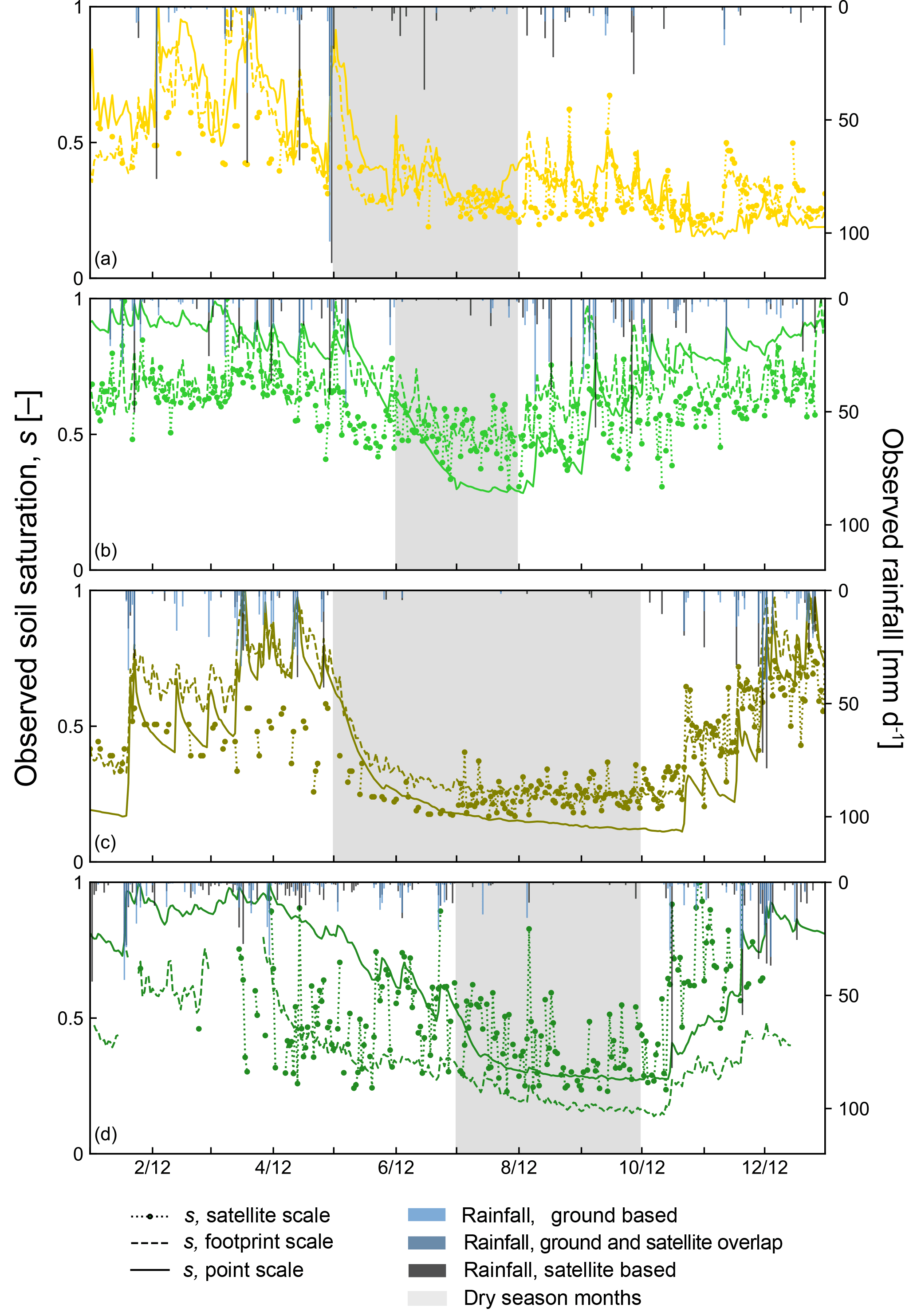
https://www.hydrol-earth-syst-sci.net/22/3229/2018/hess-22-3229-2018-f01

Figure 1Soil saturation and rainfall time series from (a) US-ARM, (b) US-MMS, (c) US-Ton, and (d) US-Me2.

Download

Table 1Selected study sites.

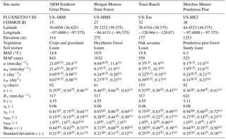
Latitude and longitude in parentheses correspond the centroid of the satellite area associated with the site location; MAT, mean annual temperature from long-term FLUXNET2015 data; MAP, mean annual precipitation from long-term FLUXNET2015 data; soil texture taken from the HWSD; n, porosity; K_s, saturated soil hydraulic conductivity; b, pore size distribution index; s_h, hydroscopic point; s_fc, field capacity; α, observed average daily rainfall depth in 2012; the subscript “w” indicates that α was computed for only the wet season months; λ, observed average daily rainfall frequency in 2012; the subscript “w” indicates that λ was computed for only the wet season months; t_d, number of days in the dry season; superscripts ^(p), ^(f), and ^(s) correspond to values used for the point-, footprint-, and satellite-scale analysis. Citations for each FLUXNET2015 site: Biraud (2002), Novick and Phillips (1999), Law (2002), and Baldocchi (2001).

Download Print Version | Download XLSX

2.2 Analytical model for soil saturation probability density functions (pdfs)

2.2.1 Model definition

Our framework is based on a standard bucket model of soil column hydrology at a point forced with stochastic precipitation inputs and in which soil water losses are a function of soil saturation. We followed the simple formulation of soil water losses in Laio et al. (2001a). We applied two associated analytical formulations for the soil saturation pdf detailed below and derived under the assumption of steady state, wherein parameters are constant for a given period of time. The annual model assumed an annual rainfall pattern and the seasonal model accounted for a wet season rainfall pattern and a dry season of negligible rainfall.

The soil water balance model is defined at a point and a daily time step, for a soil with porosity n, and assuming that soil saturation is uniform in the considered soil column of depth Z. Rainfall, the only input to the soil water balance, is treated as a Poisson distribution characterized by an average event frequency λ and average event intensity α. For simplicity, we assumed that the rainfall applied was equal to the amount that reached the ground surface and that interception by vegetation was negligible. Interception may be a significant component of the soil water balance at forested sites and may need to be considered in future extensions of this work. The daily soil water balance is the difference between the rate of rainfall infiltration φ and the rate of soil moisture losses χ :

\begin{matrix} (1) & n Z \frac{d s (t)}{d t} = φ [s (t); t] - χ [s (t)] . \end{matrix}

φ[s(t); t] is both a stochastic process controlled by rainfall and also a state-dependent process because excess rainfall relative to available soil storage is converted to surface runoff. the soil moisture loss curve, χ[s(t)], includes leakage losses due to gravity and evapotranspiration and is described in stages determined by five soil saturation thresholds (Laio et al., 2001a). These stages are: (i) the saturation point (s = 1), at which all pores are filled with water; (ii) the field capacity (s_fc), at which soil-gravity drainage becomes negligible compared to evaporation; (iii) the point of incipient stomata closure (s^*), at which plants begin to reduce transpiration from water stress; (iv) the wilting point (s_w), at which plants cease to transpire; and (v) the hydroscopic point (s_h), at which water is bound to the soil matrix. Soil water losses are controlled by physical soil properties for saturation states above s_fc. The rate of leakage due to gravity is assumed maximum when soil is saturated (K_s) and decays exponentially to zero at s_fc (Brooks and Corey, 1964). Soil water losses are controlled by micro-meteorological conditions for saturation states between s_fc and s^*. The rate of evapotranspiration is assumed to occur at a maximum rate (E_max), independent of the saturation state. Soil water losses are controlled primarily by vegetation for saturation states between s^* and s_w. Plants close their stomata in response to soil water deficits that drive leaf water potential gradients, as well as to atmospheric vapor pressure deficits, and evapotranspiration decreases linearly from E_max to E_w at s_w. Soil water losses are controlled by soil diffusivity for soil saturation states below s_w, and soil evaporation decreases linearly from E_w to zero at s_h. Soil water losses are negligible for soil saturation states below s_h. For this simplified theoretical description of the soil water loss curve and stochastic rainfall forcing, the analytical solution of the steady state probability distributions of soil saturation, p(s) , was given by Laio et al. (2001a):

\begin{matrix} (2) & p (s) = \{\begin{cases} 0, & 0 < s \leq s_{h}, \\ \frac{C}{η_{w}} {(\frac{s - s_{h}}{s_{w} - s_{h}})}^{\frac{λ (s_{w} - s_{h})}{η_{w}} - 1} e^{- γ s}, & s_{h} < s \leq s_{w}, \\ \frac{C}{η_{w}} {[1 + (\frac{η}{η_{w}} - 1) (\frac{s - s_{w}}{s^{*} - s_{w}})]}^{\frac{λ (s^{*} - s_{w})}{η - η_{w}} - 1} e^{- γ s}, & s_{w} < s \leq s^{*}, \\ \frac{C}{η} e^{- γ s + \frac{λ}{η} (s - s^{*})} {\frac{η}{η_{w}}}^{\frac{λ (s^{*} - s_{w})}{η - η_{w}}}, & s^{*} < s \leq s_{fc}, \\ \frac{C}{η} e^{- (β + γ) s + β s_{fc}} {(\frac{η e^{β s}}{(η - m) e^{β s_{fc}} + m e^{β s}})}^{\frac{λ}{β (η - m)} + 1} \\ \times {\frac{η}{η_{w}}}^{\frac{λ (s^{*} - s_{w})}{η - η_{w}} e^{\frac{λ}{η} (s_{fc} - s^{*})}}, & s_{fc} < s \leq 1, \end{cases} \end{matrix}

where

\begin{array}{l} \frac{1}{γ} = \frac{α}{n Z}, \\ η_{w} = \frac{E_{w}}{n Z}, \\ η = \frac{E_{\max}}{n Z}, \\ m = \frac{K_{s}}{n Z (e^{β (1 - s_{fc})} - 1)}, \\ β = 2 b + 4, \end{array}

where b is an experimentally determined parameter used in the Clapp and Hornberger (1978) soil water retention curve, and the constant C can be obtained numerically to ensure the integral of p(s) = 1. We used a simplifying relation E_w = 0.05E_max to reduce the number of parameters.

We adopted Dralle and Thompson's (2016) framework to account for transient dynamics between wet and dry seasons. We defined the dry season as a period of duration t_d in which precipitation was negligible and assumed to not contribute to soil moisture. During that period, we assumed soil saturation decayed from an initial value s₀ to s(t_d, s₀) given by Laio et al. (2001a). For simplicity, we determined t_d using rainfall records at a monthly step (see Sect. 2.2.2) and s₀ was the soil saturation value on the last day of the wet season. Note that we did not define s₀ as the soil saturation following the last significant storm of the wet season as was done in prior studies (Dralle and Thompson, 2016). We then calculated the annual soil saturation pdf (p_wd(s)) as the weighted sum of the wet and dry season pdfs, p_w(s) and p_d(s), respectively.

\begin{matrix} (3) & p_{wd} (s) = (1 - \frac{t_{d}}{365}) p_{w} (s) + \frac{t_{d}}{365} p_{d} (s) \end{matrix}

The steady-state solution in Eq. (2) was used for the wet season pdf and the dry season pdf is numerically determined by

\begin{matrix} (4) & p_{d} (s) = \int_{0}^{1} p_{S_{d} | S_{0}} (s, s_{0}) p_{0} (s_{0}) d s_{0}, \end{matrix}

where p₀(s₀) is the pdf of the initial dry season soil saturation, equal to p_w(s), and $p_{S_{d} | S_{0}} (s$ , s₀) is the pdf of dry season soil saturation given an initial condition s₀.

\begin{matrix} (5) & p_{S_{d} | S_{0}} (s, s_{0}) = \frac{C_{d}}{t_{d}} \{\begin{cases} \frac{e^{β (s_{0} - s)}}{(η^{d} - m) e^{β (s_{0} - s)} - η^{d} + m + m e^{β (s_{0} - s_{fc})}}, & s_{fc} < s \leq 1, \\ \frac{1}{η^{d}}, & s^{*} < s \leq s_{fc}, \\ \frac{1}{η^{d} - η_{w}^{d}} (\frac{s^{*} - s_{w}}{(η^{d} - η_{w}^{d}) (s - s_{w}) + η_{w}^{d} (s^{*} - s_{w})}), & s_{w} < s \leq s^{*} \\ \frac{1}{η_{w}^{d}} (\frac{s_{w} - s_{h}}{s - s_{h}}), & s_{h} < s \leq s_{w} \\ 0, & s_{0} \leq s, \\ 0, & s \leq s_{h}, \\ 0, & s \leq s (t_{d}, s_{0}) \end{cases} \end{matrix}

where η^d and $η_{w}^{d}$ are equivalent to η and η_w relative to $E_{\max}^{d}$ , the maximum evapotranspiration rate during the dry season, and C_d is a normalization constant. We used the analytical expression for soil saturation decay, s(t, s₀), in the absence of rainfall given by Laio et al. (2001a) to derive $p_{S_{d} | S_{0}} (s$ , s₀).

2.2.2 Climate, soil, and vegetation parameter characterization

We chose readily available data for rainfall characteristics (λ and α), length of the dry period (t_d), and physical soil parameters (s_fc, s_h, K_s, and b) needed in the analytical models of soil saturation pdfs (Eqs. 2 and 3). We focused on estimating the ecohydrological parameters s^*, s_w, and E_max, which describe vegetation control on soil water losses and are not easily observable.

We calculated rainfall characteristics λ and α for the year and wet season months for each site from FLUXNET2015 and TRMM rainfall records following Rodriguez-Iturbe et al. (1984) (Table 1). We used FLUXNET2015 rainfall characteristics for point- and footprint-scale analyses, and we used TRMM rainfall characteristics for the satellite-scale analysis. TRMM rainfall records were generally consistent with ground-based measurements. For each location, we evaluated monthly FLUXNET2015 rainfall depth and categorized consecutive months contributing < 5 % of the site's annual rainfall as dry season months (Fig. 1). We then calculated the length of the dry period (t_d) as the number of days in those dry months. We used physical soil characteristics for soil textures at each site (s_h, K_s, and b) from Rawls et al. (1982) (Table 1). We estimated s_fc from each soil saturation record (Table 1) to be consistent with the assumption that drainage losses are insignificant compared to evapotranspiration losses the day following a rain event. We identified all days in the 2012 record following an observed decrease in soil saturation and estimated s_fc as the 95th percentile of the soil saturation value of the selected days. Daily soil saturation below s_w and above s_fc is rare (Laio et al., 2001a), so we did not expect the average soil texture values for s_h and K_s to significantly affect the results. Soil depths Z are 10, 20, and 5 cm for the point, footprint, and satellite scales, respectively. E_max is only a fraction of the atmospheric moisture demand (or potential evapotranspiration) contributed by that soil depth because we used a soil depth that is shallower than the rooting depth. Consequently our framework includes four (or three if seasonality is ignored) unknown soil water balance parameters, s^*, s_w, E_max, and $E_{\max}^{d}$ . We estimated these parameters over the following intervals:

\begin{matrix} (6) & \{\begin{cases} s_{h} \leq s^{*} \leq s_{fc}, \\ s_{h} \leq s_{w} \leq s_{fc}, \\ 0 \leq E_{\max} \leq 10, \\ 0 \leq E_{\max}^{d} \leq 10, \end{cases} \end{matrix}

where 10 mm day⁻¹ is the pre-defined upper possible boundary for potential evapotranspiration.

2.3 Bayesian inversion approach

2.3.1 Application of the Bayes theorem

We related p(S), the empirical soil saturation pdf of the j = [1, …, m] soil saturation observations (s_j), and the analytical soil saturation pdfs in Eqs. (2) or (3) derived from the simple soil water balance model in Eq. (1) with up to four unknown soil water balance parameters θ = [s^*, s_w, E_max, $E_{\max}^{d}]$ using the Bayes' theorem defined as

\begin{matrix} (7) & p (θ | S) = \frac{p (S | θ) p (θ)}{p (S)}, \end{matrix}

where the posterior distribution, p(θ|S), is the solution of the inverse problem and describes the probability of model parameters θ given the set S = [s₁s₂, … s_m] of soil saturation observations. Assuming uninformed prior knowledge, the prior distribution of model parameters θ, p(θ), were defined by uniform distributions over the intervals (Eq. 6). The conditional probability of observations S given model parameters θ, p(S|θ), is the likelihood function of model parameters θ.

2.3.2 Parameter estimation

We used the Metropolis–Hastings Markov chain Monte Carlo (MH-MCMC) technique to estimate the posterior distribution of p(θ|S) by drawing random model samples θ_i from p(θ) and evaluating p(S|θ_i) (Metropolis et al., 1953; Hastings, 1970; Xu et al., 2006). We defined the likelihood function of a model i, p(S|θ_i), as

\begin{matrix} (8) & p (S | θ_{i}) = \prod_{j = 1}^{m} p (s_{j} | θ_{i}), \end{matrix}

where p(s_j|θ_i) is the probability of observation s_j given Eqs. (2) or (3) using parameters θ_i.

The MH-MCMC technique converges to a stationary distribution according to the ergodicity theorem in Markov chain theory. The sampling algorithm consisted of repeating two steps: (i) a proposing step, in which the algorithm generates a new model $θ_{i}^{'}$ using a random function that is symmetric about the previously accepted model θ_i, and (ii) a moving step, to determine whether the model should be accepted or rejected, in which $θ_{i}^{'}$ is tested against the Metropolis criterion (a) defined as

\begin{matrix} (9) & a = \frac{p (S | θ_{i}^{'})}{p (S | θ_{i})} . \end{matrix}

If a > 1, θ_i was accepted and θ_i+1 = $θ_{i}^{'}$ was used for the next sample. If a < 1, a random number p_* ∈ [0, 1] was drawn from a uniform distribution and compared to a. If p_* < a, $θ_{i}^{'}$ was accepted and θ_i+1 = $θ_{i}^{'}$ was used for the next sample. If p_* > a, $θ_{i}^{'}$ was rejected and θ_i+1 = θ_i was used for the next sample. If $θ_{i}^{'}$ was an inconsistent model in which soil saturation thresholds (s_w, s_*) were ranked incorrectly or any of the soil water balance parameters (s^*, s_w, E_max, $E_{\max}^{d}$ ) were outside of their defined physical bounds, the model likelihood was zero and $θ_{i}^{'}$ was never accepted. The log-likelihood was more convenient to compute than the likelihood. The symmetric function used in the proposing step was a Gaussian distribution with a mean value equal to the accepted model θ_i and a standard deviation of 1 % of interval range for which each parameter is defined in Eq. (6). We selected this value of the standard deviation of each model parameter after a number of test runs to generally ensure an acceptance rate between 20 and 50 % (Roberts and Rosenthal, 2001). We obtained statistics of the estimated parameters in θ from the union of three run samples of 20 000 simulations each. The burn-in period is the number of simulations after which the running mean and standard deviation are stabilized. We considered a burn-in period of 10,000 simulations, which were discarded for each run sample. If the acceptance rate of a run sample was < 1 or > 90 % after the burn-in period, we discarded the run and concluded that the algorithm was stuck in a local minimum that might be physically impossible. We evaluated convergence by the Gelman–Rubin (GR) diagnostic (Gelman and Rubin, 1992) on the run samples. The GR diagnostic determines that the algorithm reaches convergence when the within-run variability (σ_w) is roughly equal to the between-run variability (σ_b), that is, when σ_w∕σ_b approaches one. We verified that the GR diagnostic for each estimated parameter was < 1.1. If the GR diagnostic did not indicate that the three run samples converged, we discarded the run with the lowest likelihood and re-initiated a new run sample until convergence was attained. We counted the number of attempts to quantify how rapidly convergence occurred. We computed mean and standard deviation for each parameter from a total of 30 000 simulations of θ resulting from the three converging run samples. A mean analytical model of soil saturation pdf was determined by applying Eqs. (2) or (3) with the mean values of the 30 000 posterior parameter estimates.

2.4 Model evaluation criteria

We did not have direct measurement to validate the parameters s^*, s_w, and E_max estimated through the Bayesian inversion methods. We therefore analysed convergence and uncertainty metrics of the model inversion and goodness of fit between empirical and analytical soil saturation pdfs to evaluate the identifiability of the ecohydrological parameters. We compared the optimum analytical pdf derived from the mean parameter estimates and the empirical pdfs derived from observations. We evaluated the model inversion using the following criteria:

i.
Convergence of the Bayesian inversion: a GR diagnostic < 1.1 for all unknown parameters is obtained from the union of three run samples and within ≤ 10 sample runs.
ii.
Low uncertainty in parameter estimates: the posterior distributions of parameter estimates are physically plausible and have coefficients of variations < 20 %.
iii.
Goodness of fit: a quantile-level Nash–Sutcliffe efficiency (NSE) (Müller et al., 2014) > 0.85 and a Kolmogorov–Smirnov statistic < 0.2.

2.5 Method assessment

Major assumptions and limitations embedded in the proposed inference framework were tested through the analysis detailed below. We assume, for each scale and location, that the shape of empirical the soil saturation pdfs is controlled by the physical constraints used to parameterize the analytical model of soil saturation pdfs, these parameters can be determined with some certainty and reflect variability in soil water dynamics. We expect that estimated soil saturation thresholds have greater certainty when the empirical soil saturation pdf is defined around those values and greater uncertainty when fewer soil saturation values are observed around the thresholds. We acknowledge that pre-defined rainfall characteristics and physical soil parameters based on observations or literature values may not be exactly representative of the processes at each location or scale and could also create biases and uncertainties in the fitted parameters of interest. We used model evaluation criteria (Sect. 2.4) to investigate the applicability of the inference framework with varying model complexities, scales, locations and data availability.

i.
Analytical expressions for soil saturation pdfs were derived under the assumption of steady state. Annual soil moisture records can be affected by transitional dynamics between wet and dry seasons, and the appropriate level of model complexity must be used. We applied the inversion framework to annual soil saturation using variations of the analytical model for soil saturation pdfs of increasing complexity: (i) the annual model in Eq. (2) and (ii) the seasonal model in Eq. (3). We determined whether the added complexity of the dry season pdf increases the identifiability of ecohydrological parameters or if the simpler annual model is sufficiently consistent with annual empirical soil saturation pdfs.
ii.
We compared co-located parameter estimates and their uncertainty at point, footprint, and satellite scales for each site. We determine whether the inference approach can provide appropriate scale-specific parameters for ecohydrological modeling at each location.
iii.
We assumed that the whole range of realizable soil saturation values was captured within the selected time series at each scale and that the resulting soil saturation pdf was not truncated. If the range of observed values is not representative of the soil saturation pdf because it is truncated or affected by noise in the data, parameter estimates may be biased. Minimum and maximum observed soil saturation values during 2012 (Table 1) indicate the range of observed soil saturation values we used to estimate ecohydrological parameters. We determine whether the inference method based on soil saturation pdfs is robust against reduced data availability by repeating the model inversions on subsets of the soil saturation time series and show that the method can be applied to sparse datasets. We performed the model inversion using subsets of each soil saturation record by randomly resampling fractions of the data down to 10 % of the annual timeseries and computed goodness of fit statistics between the resulting analytical models and the empirical models based on the full annual record. We determined the number of data points necessary to infer converging model parameters that best match observations and whether the proposed inference method based on soil saturation pdf can be reliably used to identify ecohydrological parameters from sparse datasets.

Table 2Estimated ecohydrological parameters and goodness of fit of analytical soil saturation pdfs.

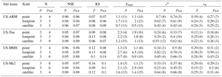
Values in parentheses correspond to the coefficient of variation of the posterior parameter estimates in percentage. p, analytical model for the soil saturation pdf without seasons, p_wd, analytical model for the soil saturation pdf including wet and dry seasons; N, number of 20 000 simulation runs needed to obtain three converging results (see Sect. 2.3.2); NSE, quantile-level Nash–Sutcliffe efficiency; KS, Kolmogorov–Smirnov statistic; E_max, maximum evapotranspiration in mm day⁻¹ (the weighted average wet and dry season E_max is reported for the p_wd model); s^*, point of incipient stomatal closure; s_w, wilting point.

Download Print Version | Download XLSX

3 Results and discussion

3.1 Level of model complexity

For each of the four locations (Table 1), we obtained optimal analytical soil saturation pdfs consistent with the empirical pdfs derived from soil saturation observations using the Bayesian inversion framework and a MH-MCMC algorithm. Model inversions for each site and scale and for both annual and seasonal models met the evaluation criteria (see Sect. 2.4). Our results indicated that the framework of Dralle and Thompson (2016) can be applied to sites with low (US-MMS) and high (US-Ton) seasonality in rainfall patterns. Posterior probability distributions of soil water balance parameters (s_w, s^*, E_max) were well constrained overall. The parameter estimates and their coefficient of variation as well as the model goodness of fit statistics are summarized in Table 2. Figures 2 through 5 present a comparison between empirical as well as analytical pdfs and associated quantile–quantile plots for point, footprint, and satellite scales at the four study sites and for both annual and seasonal models. The goodness of fit between empirical pdfs and analytical models was only slightly better for the seasonal model than for the annual model. However, the coefficient of variation of the posterior parameter distributions was smaller for the annual model and it converged more rapidly. The Bayesian inversion of the annual model is therefore more computationally efficient. The parameter identifiability was not greatly improved by the more complex seasonal model. The estimated soil saturation threshold s_w was consistently smaller for the annual model than for the seasonal model and s^* was often higher, which may indicate that s_w and s^* in the annual model could be biased and may have absorbed dry season dynamics. Previous studies calibrating soil saturation pdf models found ecohydrological parameter values comparable to ours (Table 2). For example, using point-scale observations at US-Ton, best-fit values of s_w and s_fc were 0.26 and 0.82, respectively (Dralle and Thompson, 2016), and best-fit values of s^* and E_max were 0.3 and 1.9 mm day⁻¹, respectively (Miller et al., 2007). We did not compare soil saturation thresholds s^* and s_w with literature values of soil water potential at which stomata are fully open or closed because the conversion of soil saturation to soil matrix potential is non-linear (Clapp and Hornberger, 1978) and site- and scale-specific soil water retention parameters were unknown. Average parameters derived from soil texture (Rawls et al., 1982) were not compatible with soil moisture data from each scale and site.

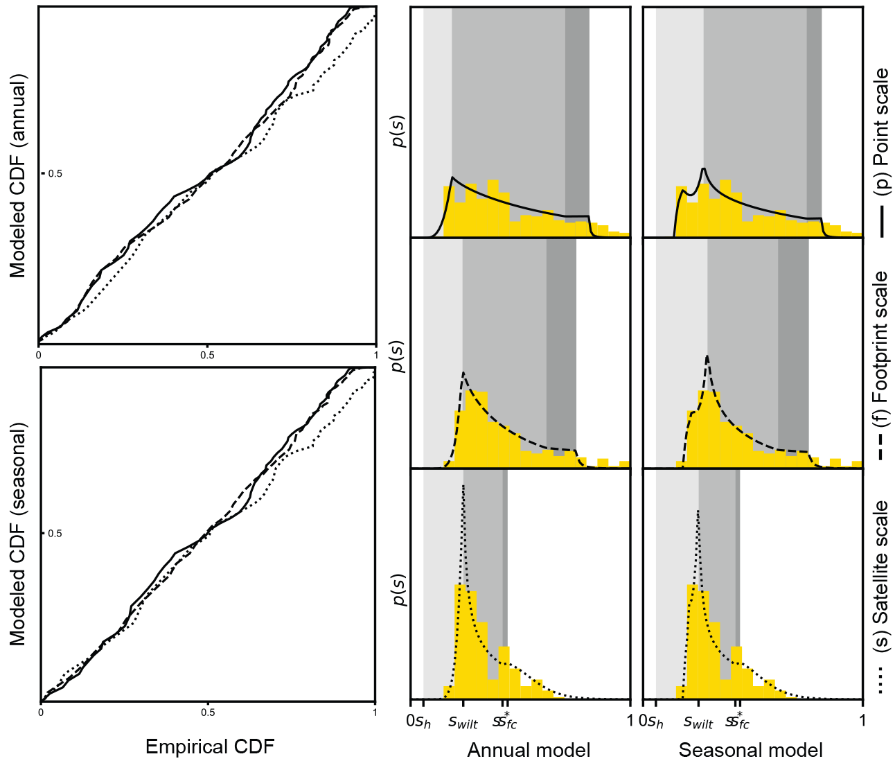
https://www.hydrol-earth-syst-sci.net/22/3229/2018/hess-22-3229-2018-f02

Figure 2Empirical versus modeled cumulative density functions (CDFs) and soil saturation probability distribution (p(s)) for US-ARM. The mean values of the posterior parameter distributions were used with Eq. (2) in the annual model and Eq. (3) in the seasonal model. The grey shaded areas correspond to the soil saturation thresholds (s_h, s_w, s^*, s_fc) in the water balance model.

Download

https://www.hydrol-earth-syst-sci.net/22/3229/2018/hess-22-3229-2018-f03

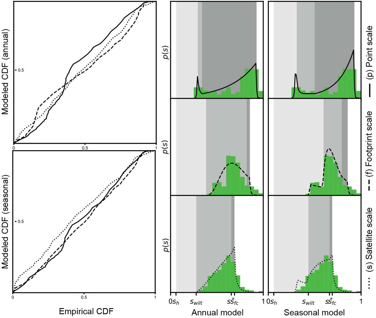
Figure 3Empirical versus modeled CDFs and soil saturation probability distribution (p(s)) for US-MMS. The mean values of the posterior parameter distributions were used with Eq. (2) in the annual model and Eq. (3) in the seasonal model. The grey shaded areas correspond to the soil saturation thresholds (s_h, s_w, s^*, s_fc) in the water balance model.

Download

https://www.hydrol-earth-syst-sci.net/22/3229/2018/hess-22-3229-2018-f04

Figure 4Empirical versus modeled CDFs and soil saturation probability distribution (p(s)) for US-Ton. The mean values of the posterior parameter distributions were used with Eq. (2) in the annual model and Eq. (3) in the seasonal model. The grey shaded areas correspond to the soil saturation thresholds (s_h, s_w, s^*, s_fc) in the water balance model.

Download

https://www.hydrol-earth-syst-sci.net/22/3229/2018/hess-22-3229-2018-f05

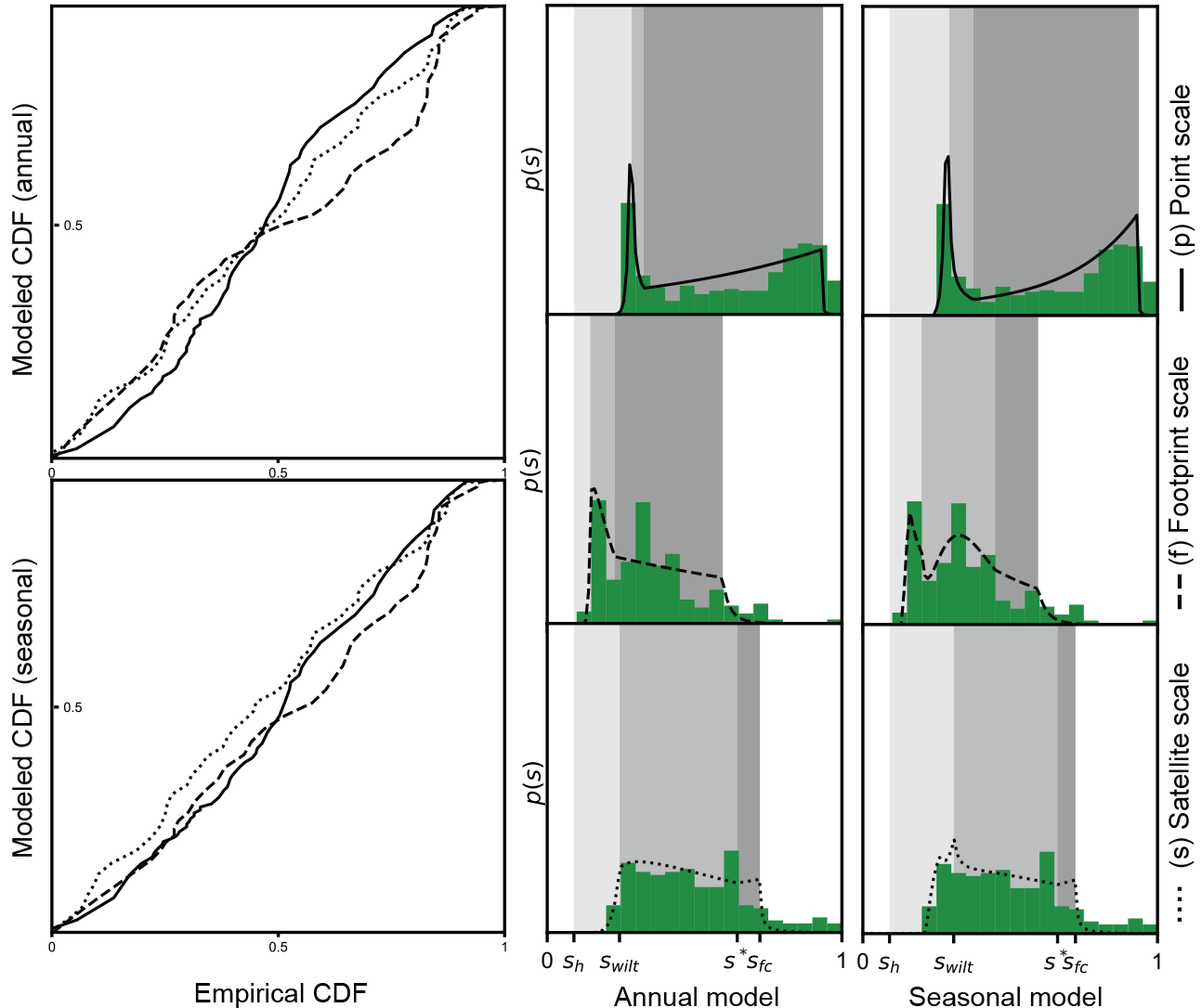
Figure 5Empirical versus modeled CDFs and soil saturation probability distribution (p(s)) for US-Me2. The mean values of the posterior parameter distributions were used with Eq. (2) in the annual model and Eq. (3) in the seasonal model. The grey shaded areas correspond to the soil saturation thresholds (s_h, s_w, s^*, s_fc) in the water balance model.

Download

https://www.hydrol-earth-syst-sci.net/22/3229/2018/hess-22-3229-2018-f06

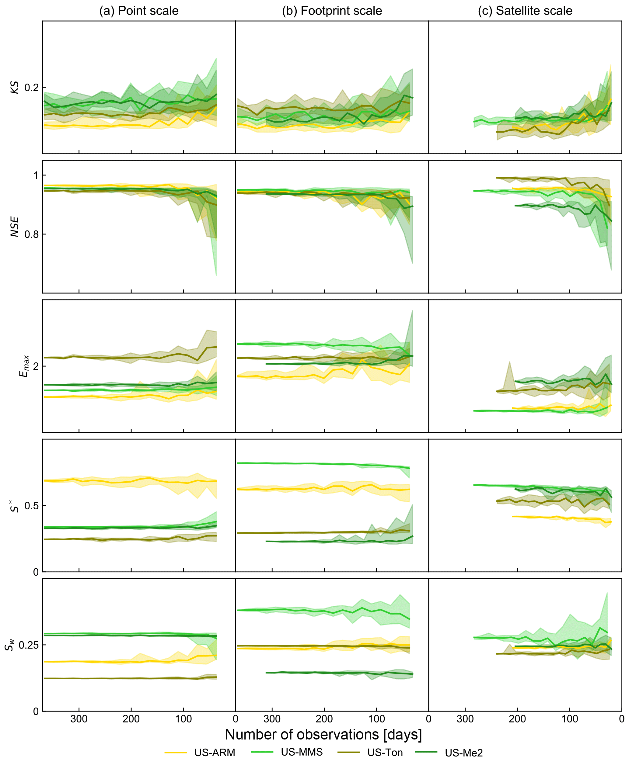
Figure 6Goodness of fit and ecohydrological parameters inferred with decreasing number of soil saturation observations (annual model). For each subsample category, the median results of 10 repeats are plotted and results between the 90th and 10th percentiles are shaded. Colors correspond to the four sites in the legend. KS, Kolmogorov–Smirnov statistic; NSE, quantile-level Nash–Sutcliffe efficiency; E_max, maximum evapotranspiration in mm day⁻¹; s^*, point of incipient stomatal closure; s_w, wilting point.

Download

3.2 Site and scale considerations

Parameter estimates were most constrained for scales and locations at which soil water dynamics are more sensitive to the fitted ecohydrological parameters of interest. In these cases, convergence of the model inversion was attained less rapidly, but ultimately provided better goodness of fit. Soil saturation states at drier sites may be more controlled by soil water loss parameters, while soil saturation states at wetter sites may also be controlled by rainfall characteristics. Estimated soil saturation thresholds had greater certainty if the empirical soil saturation pdfs were defined around those values and had greater uncertainty if there were fewer soil saturation values observed around the thresholds. For example, uncertainty of s_w was greater for the humid subtropical deciduous forest site (US-MMS) than for the Mediterranean savanna sites (US-Ton), and uncertainty of s^* was greater for US-Ton than US-MMS. Similarly, soil saturation states representing larger spatial scales were less sensitive to specific site characteristics.

Parameter uncertainty for satellite and footprint scales was greater than for the point scale. Estimates of larger-scale soil water balance parameters are more relevant to regional ecohydrological dynamics. Differences in parameter estimates among scales within a site may be associated with differences in soil texture properties, such as porosity and field capacity, that were determined separately for each record. Co-located and concurrent soil saturation pdfs are different at each scale (Figs. 2–5) and suggest variability in observed soil water dynamics at each scale. Differences in driving processes among scales were specifically determined from the model inversion for each scale and provided robust scale-specific parameters for ecohydrological modeling.

3.3 Data availability

For each spatial scale and site, the annual model was inversed, using random subsamples of 100 to 10 % of the 2012 time series (Fig. 6). For all sites and scales the number of observations did not significantly impact model inference. The NSE, Kolmogorov–Smirnov statistic, and parameter estimates were stable down to about 100 observations. Fitted model parameter values and the variability of parameter estimates among the 10 repetitions in each subsample category were not sensitive to the number of observations used. Results indicate the identifiability of ecohydrological parameters through the inversion of the analytical model of soil saturation pdfs was robust because the mean and standard deviation of the randomly selected subsets of annual data were representative of the full record. There was no correlation between the small differences in the mean and standard deviations of the subsamples and the model goodness of fit. The proposed inference method based on soil saturation pdfs can therefore reliably be used to identify ecohydrological parameters from sparse datasets. Inference methods, which do not require continuous data, are particularly relevant to large-scale soil moisture measurements, such as satellite products, that are not continuous.

4 Conclusions

We document a generalizable Bayesian inversion framework to infer parameter values of the stochastic soil water balance model and their associated uncertainty using freely available rainfall and soil moisture observations at point-, footprint- and satellite-scales. Empirical pdfs derived from soil saturation observations provided key information to determine unknown ecohydrological parameters s^*, s_w, and E_max. Model assumptions were appropriately met, and optimal analytical soil saturation pdfs were consistent with empirical pdfs. Uncertainty in parameter estimates were small and reflected the sensitivity of the soil water balance model to ecohydrological parameters at varying scales and locations. We demonstrate that the form of the simple ecohydrological model for soil saturation pdfs was consistent with observations from point-, footprint-, and satellite-scales. However, optimal parameters were different at each scale because co-located and concurrent soil saturation pdfs are different at each scale, which may result from spatial heterogeneity in soil water dynamics. We demonstrate the advantage of analyzing soil saturation pdfs instead of time series. We obtained stable results using sparse subsets of the datasets, indicating that the proposed framework is robust and can be used with non-continuous data. Although the seasonal model was conceptually more consistent with our physical understanding of annual soil water dynamics, the annual model provided satisfactory results matching annual empirical pdf sites we analysed. We were not able to determine if some differences in parameters estimated using the seasonal model are physically meaningful because wet and dry season dynamics were better characterized in this more complex model. Our methodology can be customized to characterize site-specific parameters and to test consistency between observed and analytical soil saturation pdfs for any other adaptation of the stochastic ecohydrological framework with more or less complexity depending on the study objectives.

We provide a method based on a parsimonious soil water balance model, requiring a minimum level of data inputs to estimate ecohydrological characteristics that are not directly observable and for which established estimation methods are not available. Our methods can be applied in future studies to better understand differences in soil water dynamics at different scales and to improve scaling of ecohydrological processes. Results demonstrate the value of large-scale near-surface soil moisture observations to improve characterization of soil water dynamics at ecosystem scales. Relations between the soil saturation threshold values inferred from the near-surface soil moisture data and dynamics in the full active rooting zone are unknown. The datasets we used are freely available from sensor networks and global satellite products, and methods can therefore be applied to a large range of sites or to global analyses to improve understanding of spatial patterns in ecohydrological parameters relevant for local and global water cycle analyses.

Code and data availability

We downloaded all datasets from publicly available sources. Point-scale soil moisture and rainfall data are available through FLUXNET2015 (http://fluxnet.fluxdata.org/data/fluxnet2015-dataset/); footprint-scale soil moisture data are available through COSMOS (http://cosmos.hwr.arizona.edu/Probes/probelist.html); remotely sensed soil moisture data are available through ESA CCI (http://www.esa-soilmoisture-cci.org/node/145); remotely sensed rainfall data are available through NASA TRMM (https://pmm.nasa.gov/data-access/downloads/trmm); global soil texture data are available through FAO HWSD (http://www.fao.org/soils-portal/soil-survey/soil-maps-and-databases/harmonized-world-soil-database-v12/en/). Custom scripts in the Python computing language associated with our analysis are open source (Bassiouni, 2018, https://doi.org/10.5281/zenodo.1283371).

Competing interests

The authors declare that they have no conflict of interest.

Acknowledgements

We thank Minghui Zhang, Marc Müller, David Dralle, Xue Feng, and editor Sally Thomspon for their thoughtful reviews and useful feedback on an earlier draft of this paper. This material is based upon work supported by the National Science Foundation Graduate Research Fellowship under grant no. 1314109-DGE. Stephen P. Good acknowledges the financial support of the US National Aeronautics and Space Administration (NNX16AN13G). This work used the Extreme Science and Engineering Discovery Environment (XSEDE) via allocation DEB160018, supported by National Science Foundation grant number ACI-1548562. This work used data acquired and shared by the FLUXNET community, including these networks: AmeriFlux, AfriFlux, AsiaFlux, CarboAfrica, CarboEuropeIP, CarboItaly, CarboMont, ChinaFlux, Fluxnet-Canada, GreenGrass, ICOS, KoFlux, LBA, NECC, OzFlux-TERN, TCOS-Siberia, and USCCC. The FLUXNET eddy covariance data processing and harmonization were carried out by the European Fluxes Database Cluster, AmeriFlux Management Project, and Fluxdata project of FLUXNET, with the support of CDIAC and the ICOS Ecosystem Thematic Center and the OzFlux, ChinaFlux, and AsiaFlux offices.

Edited by: Sally Thompson
Reviewed by: Xue Feng, David Dralle, Marc F. Muller, and Minghui Zhang

References

Baldocchi, D.: AmeriFlux US-Ton Tonzi Ranch, https://doi.org/10.17190/AMF/1245971, 2001.

Baldwin, D., Manfreda, S., Keller, K., and Smithwick, E. A. H.: Predicting root zone soil moisture with soil properties and satellite near-surface moisture data across the conterminous United States, J. Hydrol., 546, 393–404, https://doi.org/10.1016/j.jhydrol.2017.01.020, 2017.

Bassiouni, M.: PIEP, https://doi.org/10.5281/zenodo.1283371, 2018.

Biraud, S.: Ameriflux US-ARM ARM Southern Great Plains site-Lamont, https://doi.org/10.17190/AMF/1246027, 2002.

Brooks, R. and Corey, T.: Hydraulic properties of porous media, hydrology papers, Colorado State University, 1964.

Caylor, K. K., D'Odorico, P., and Rodriguez-Iturbe, I.: On the ecohydrology of structurally heterogeneous semiarid landscapes, Water Resour. Res., 42, W07424, https://doi.org/10.1029/2005WR004683, 2006.

Chen, X., Rubin, Y., Ma, S., and Baldocchi, D.: Observations and stochastic modeling of soil moisture control on evapotranspiration in a Californian oak savanna: soil moisture control on ET, Water Resour. Res., 44, W08409, https://doi.org/10.1029/2007WR006646, 2008.

Clapp, R. B. and Hornberger, G. M.: Empirical equations for some soil hydraulic properties, Water Resour. Res., 14, 601–604, 1978.

COSMOS Dataset, http://cosmos.hwr.arizona.edu/Probes/probelist.html, last access: 4 August 2016.

Dorigo, W. A., Gruber, A., De Jeu, R. A. M., Wagner, W., Stacke, T., Loew, A., Albergel, C., Brocca, L., Chung, D., Parinussa, R. M., and Kidd, R.: Evaluation of the ESA CCI soil moisture product using ground-based observations, Remote Sens. Environ., 162, 380–395, https://doi.org/10.1016/j.rse.2014.07.023, 2015.

Dralle, D. N. and Thompson, S. E.: A minimal probabilistic model for soil moisture in seasonally dry climates, Water Resour. Res., 52, 1507–1517, https://doi.org/10.1002/2015WR017813, 2016.

Dralle, D. N., Karst, N. J., and Thompson, S. E.: Dry season streamflow persistence in seasonal climates, Water Resour. Res., 52, 90–107, https://doi.org/10.1002/2015WR017752, 2016.

FAO/IIASA/ISRIC/ISS-CAS/JRC: Harmonized World Soil Database (version 1.1), FAO, Rome, Italy and IIASA, Laxenburg, Austria, 2009.

Feng, X., Dawson, T. E., Ackerly, D. D., Santiago, L. S., and Thompson, S. E.: Reconciling seasonal hydraulic risk and plant water use through probabilistic soil-plant dynamics, Global Change Biol., 23, 3758–3769, https://doi.org/10.1111/gcb.13640, 2017.

FLUXNET2015 Dataset: http://fluxnet.fluxdata.org/data/fluxnet2015-dataset/, last access: 22 October 2016.

Gelman, A. and Rubin, D. B.: Inference from iterative simulation using multiple sequences, Stat. Sci., 7, 457–472, 1992.

Global Soil Moisture Dataset (ESA CCI SM v04.2): http://www.esa-soilmoisture-cci.org/node/145, last access: 21 February 2016.

Good, S. P., Soderberg, K., Guan, K., King, E. G., Scanlon, T. M., and Caylor, K. K.: δ²H isotopic flux partitioning of evapotranspiration over a grass field following a water pulse and subsequent dry down, Water Resour. Res., 50, 1410–1432, https://doi.org/10.1002/2013WR014333, 2014.

Good, S. P., Noone, D., and Bowen, G.: Hydrologic connectivity constrains partitioning of global terrestrial water fluxes, Science, 349, 175–177, 2015.

Good, S. P., Moore, G. W., and Miralles, D. G.: A mesic maximum in biological water use demarcates biome sensitivity to aridity shifts, Nat. Ecol. Evol., 1, 1883–1888, https://doi.org/10.1038/s41559-017-0371-8, 2017.

Harmonized World Soil Database v 1.2: http://www.fao.org/soils-portal/soil-survey/soil-maps-and-databases/harmonized-world-soil-database-v12/en/, last access: 21 February 2016.

Hastings, W. K.: Monte Carlo Sampling Methods Using Markov Chains and Their Applications, Biometrika, 57, 97–109, https://doi.org/10.2307/2334940, 1970.

Huffman, G. J., Bolvin, D. T., Nelkin, E. J., Wolff, D. B., Adler, R. F., Gu, G., Hong, Y., Bowman, K. P., and Stocker, E. F.: The TRMM Multisatellite Precipitation Analysis (TMPA): Quasi-Global, Multiyear, Combined-Sensor Precipitation Estimates at Fine Scales, J. Hydrometeorol., 8, 38–55, https://doi.org/10.1175/JHM560.1, 2007.

King, E. G. and Caylor, K. K.: Ecohydrology in practice: strengths, conveniences, and opportunities, Ecohydrology, 4, 608–612, https://doi.org/10.1002/eco.248, 2011.

Köhli, M., Schrön, M., Zreda, M., Schmidt, U., Dietrich, P., and Zacharias, S.: Footprint characteristics revised for field-scale soil moisture monitoring with cosmic-ray neutrons, Water Resour. Res., 51, 5772–5790, https://doi.org/10.1002/2015WR017169, 2015.

Laio, F., Porporato, A., Ridolfi, L., and Rodriguez-Iturbe, I.: Plants in water-controlled ecosystems: active role in hydrologic processes and response to water stress: II. Probabilistic soil moisture dynamics, Adv. Water Resour., 24, 707–723, 2001a.

Laio, F., Porporato, A., Fernandez-Illescas, C. P., and Rodriguez-Iturbe, I.: Plants in water-controlled ecosystems: active role in hydrologic processes and response to water stress: IV. Discussion of real cases, Adv. Water Resour., 24, 745–762, 2001b.

Laio, F., D'Odorico, P., and Ridolfi, L.: An analytical model to relate the vertical root distribution to climate and soil properties: vertical root distribution, Geophys. Res. Lett., 33, L18401, https://doi.org/10.1029/2006GL027331, 2006.

Law, B.: AmeriFlux US-Me2 Metolius mature ponderosa pine, https://doi.org/10.17190/AMF/1246076, 2002.

Li, Y., Guan, K., Gentine, P., Konings, A. G., Meinzer, F. C., Kimball, J. S., Xu, X., Anderegg, W. R. L., McDowell, N. G., Martínez-Vilalta, J., Long, D. G., and Good, S. P.: Estimating global ecosystem iso/anisohydry using active and passive microwave satellite data, J. Geophys. Res.-Biogeo., 122, 3306–3321, https://doi.org/10.1002/2017JG003958, 2017.

Liu, Y. Y., Parinussa, R. M., Dorigo, W. A., De Jeu, R. A. M., Wagner, W., van Dijk, A. I. J. M., McCabe, M. F., and Evans, J. P.: Developing an improved soil moisture dataset by blending passive and active microwave satellite-based retrievals, Hydrol. Earth Syst. Sci., 15, 425–436, https://doi.org/10.5194/hess-15-425-2011, 2011.

Liu, Y. Y., Dorigo, W. A., Parinussa, R. M., de Jeu, R. A. M., Wagner, W., McCabe, M. F., Evans, J. P., and van Dijk, A. I. J. M.: Trend-preserving blending of passive and active microwave soil moisture retrievals, Remote Sens. Environ., 123, 280–297, https://doi.org/10.1016/j.rse.2012.03.014, 2012.

Manfreda, S., Caylor, K. K., and Good, S. P.: An ecohydrological framework to explain shifts in vegetation organization across climatological gradients: Vegetation pattern in dry environments, Ecohydrology, 10, e1809, https://doi.org/10.1002/eco.1809, 2017.

Manzoni, S., Vico, G., Katul, G., Palmroth, S., and Porporato, A.: Optimal plant water-use strategies under stochastic rainfall, Water Resour. Res., 50, 5379–5394, https://doi.org/10.1002/2014WR015375, 2014.

McColl, K. A., Wang, W., Peng, B., Akbar, R., Short Gianotti, D. J., Lu, H., Pan, M., and Entekhabi, D.: Global characterization of surface soil moisture drydowns:, Geophys. Res. Lett., 44, 3682–3690, https://doi.org/10.1002/2017GL072819, 2017.

Metropolis, N., Rosenbluth, A. W., Rosenbluth, M. N., Teller, A. H., and Teller, E.: Equation of State Calculations by Fast Computing Machines, J. Chem. Phys., 21, 1087–1092, https://doi.org/10.1063/1.1699114, 1953.

Miller, G. R., Baldocchi, D. D., Law, B. E., and Meyers, T.: An analysis of soil moisture dynamics using multi-year data from a network of micrometeorological observation sites, Adv. Water Resour., 30, 1065–1081, https://doi.org/10.1016/j.advwatres.2006.10.002, 2007.

Müller, M. F., Dralle, D. N., and Thompson, S. E.: Analytical model for flow duration curves in seasonally dry climates, Water Resour. Res., 50, 5510–5531, https://doi.org/10.1002/2014WR015301, 2014.

Novick, K. and Phillips, R.: AmeriFlux US-MMS Morgan Monroe State Forest, https://doi.org/10.17190/AMF/1246080, 1999.

Porporato, A., Daly, E., and Rodriguez-Iturbe, I.: Soil water balance and ecosystem response to climate change, Am. Nat., 164, 625–632, 2004.

Rawls, W. J., Brakensiek, D. L., and Saxtonn, K. E.: Estimation of soil water properties, T. ASAE, 25, 1316–1320, 1982.

Roberts, G. O. and Rosenthal, J. S.: Optimal Scaling for Various Metropolis-Hastings Algorithms, Stat. Sci., 16, 351–367, 2001.

Rodriguez-Iturbe, I., Gupta, V. K., and Waymire, E.: Scale considerations in the modeling of temporal rainfall, Water Resour. Res., 20, 1611–1619, 1984.

Rodriguez-Iturbe, I., Porporato, A., Ridolfi, L., Isham, V., and Coxi, D. R.: Probabilistic modelling of water balance at a point: the role of climate, soil and vegetation, P. Roy. Soc. Lond. A, 455, 3789–3805, 1999.

Rodriguez-Iturbe, I., Porporato, A., Laio, F., and Ridolfi, L.: Intensive or extensive use of soil moisture: plant strategies to cope with stochastic water availability, Geophys. Res. Lett., 28, 4495–4497, 2001.

Saleem, J. A. and Salvucci, G. D.: Comparison of soil wetness indices for inducing functional similarity of hydrologic response across sites in Illinois, J. Hydrometeorol., 3, 80–91, 2002.

Salvucci, G. D.: Estimating the moisture dependence of root zone water loss using conditionally averaged precipitation, Water Resour. Res., 37, 1357–1365, 2001.

Suweis, S., Rinaldo, A., Van der Zee, S. E. A. T. M., Daly, E., Maritan, A., and Porporato, A.: Stochastic modeling of soil salinity, Geophys. Res. Lett., 37, L07404, https://doi.org/10.1029/2010GL042495, 2010.

Teuling, A. J., Seneviratne, S. I., Williams, C., and Troch, P. A.: Observed timescales of evapotranspiration response to soil moisture, Geophys. Res. Lett., 33, L23403, https://doi.org/10.1029/2006GL028178, 2006.

Thompson, S., Levin, S., and Rodriguez-Iturbe, I.: Linking Plant Disease Risk and Precipitation Drivers: A Dynamical Systems Framework, Am. Nat., 181, E1–E16, https://doi.org/10.1086/668572, 2013.

TRMM – Tropical Rainfall Measuring Mission Dataset: https://pmm.nasa.gov/data-access/downloads/trmm, last access: 21 February 2016.

Tuttle, S. E. and Salvucci, G. D.: A new approach for validating satellite estimates of soil moisture using large-scale precipitation: Comparing AMSR-E products, Remote Sens. Environ., 142, 207–222, https://doi.org/10.1016/j.rse.2013.12.002, 2014.

Volo, T. J., Vivoni, E. R., Martin, C. A., Earl, S., and Ruddell, B. L.: Modelling soil moisture, water partitioning, and plant water stress under irrigated conditions in desert urban areas, Ecohydrology, 7, 1297–1313, https://doi.org/10.1002/eco.1457, 2014.

Wagner, W., Dorigo, W., de Jeu, R., Fernandez, D., Benveniste, J., Haas, E., and Ertl, M.: Fusion of active and passive microwave observations to create an essential climate variable data record on soil moisture, ISPRS Annals of the Photogrammetry, Remote Sensing and Spatial Information Sciences (ISPRS Annals), 7, 315–321, 2012.

Wang, T., Franz, T. E., Yue, W., Szilagyi, J., Zlotnik, V. A., You, J., Chen, X., Shulski, M. D., and Young, A.: Feasibility analysis of using inverse modeling for estimating natural groundwater recharge from a large-scale soil moisture monitoring network, J. Hydrol., 533, 250–265, https://doi.org/10.1016/j.jhydrol.2015.12.019, 2016.

Whitney, K. M., Vivoni, E. R., Duniway, M. C., Bradford, J. B., Reed, S. C., and Belnap, J.: Ecohydrological role of biological soil crusts across a gradient in levels of development, Ecohydrology, 10, e1875, https://doi.org/10.1002/eco.1875, 2017.

Xu, T., White, L., Hui, D., and Luo, Y.: Probabilistic inversion of a terrestrial ecosystem model: Analysis of uncertainty in parameter estimation and model prediction, Global Biogeochem. Cy., 20, GB2007, https://doi.org/10.1029/2005GB002468, 2006.