the Creative Commons Attribution 4.0 License.
the Creative Commons Attribution 4.0 License.
 | 28 Jun 2018
The temporally varying roles of rainfall, snowmelt and soil moisture for debris flow initiation in a snow-dominated system
Karin Mostbauer
Roland Kaitna
David Prenner
Markus Hrachowitz
Debris flows represent frequent hazards in mountain regions. Though significant effort has been made to predict such events, the trigger conditions as well as the hydrologic disposition of a watershed at the time of debris flow occurrence are not well understood. Traditional intensity-duration threshold techniques to establish trigger conditions generally do not account for distinct influences of rainfall, snowmelt, and antecedent moisture. To improve our knowledge on the connection between debris flow initiation and the hydrologic system at a regional scale, this study explores the use of a semi-distributed conceptual rainfall–runoff model, linking different system variables such as soil moisture, snowmelt, or runoff with documented debris flow events in the inner Pitztal watershed, Austria. The model was run on a daily basis between 1953 and 2012. Analysing a range of modelled system state and flux variables at days on which debris flows occurred, three distinct dominant trigger mechanisms could be clearly identified. While the results suggest that for 68 % (17 out of 25) of the observed debris flow events during the study period high-intensity rainfall was the dominant trigger, snowmelt was identified as the dominant trigger for 24 % (6 out of 25) of the observed debris flow events. In addition, 8 % (2 out of 25) of the debris flow events could be attributed to the combined effects of low-intensity, long-lasting rainfall and transient storage of this water, causing elevated antecedent soil moisture conditions. The results also suggest a relatively clear temporal separation between the distinct trigger mechanisms, with high-intensity rainfall as a trigger being limited to mid- and late summer. The dominant trigger in late spring/early summer is snowmelt. Based on the discrimination between different modelled system states and fluxes and, more specifically, their temporally varying importance relative to each other, this exploratory study demonstrates that already the use of a relatively simple hydrological model can prove useful to gain some more insight into the importance of distinct debris flow trigger mechanisms. This highlights in particular the relevance of snowmelt contributions and the switch between mechanisms during early to mid-summer in snow-dominated systems.
- Article
(2795 KB) -
Supplement
(497 KB) - BibTeX
- EndNote


Debris flows are rapidly flowing mixtures of sediment and water transiting steep channels (Hungr et al., 2014) and often represent a severe hazard in mountain regions. In Alpine regions the mechanism of debris flow initiation typically ranges from distinct slope failures transforming into a flow-like movement to intensive sediment bulking due to channel erosion (e.g. Rickenmann and Zimmermann, 1993; Prancevic et al., 2014). Hereafter we refer to debris flows as channel-based mass flows that can be triggered by either landsliding or channel erosion. In contrast to the effect of a region's geomorphological and geological disposition to debris flows (e.g. Nandi and Shakoor, 2008; von Ruette et al., 2011) and in spite of significant efforts in the past (e.g. Guzzetti et al., 2008), neither the effect of hydrologic disposition (i.e. the general wetness state) of a specific region at the time of debris flow initiation nor the actual triggering hydro-meteorological conditions are well understood. Reliable regional predictions of debris flow events so far therefore remain essentially elusive.
There is a widespread consensus that high-intensity, short-duration rainfall is the primary trigger of debris flows in Alpine environments (e.g. Berti et al., 1999; Marchi et al., 2002; McArdell et al., 2007; McCoy et al., 2012; Kean et al., 2013), while longer-duration precipitation is of minor but not negligible importance (e.g. Moser and Hohensinn, 1983; Stoffel et al., 2011). However, little is known about the influence of other factors such as snowmelt or the antecedent soil moisture, which may increase a catchment's susceptibility to debris flow initiation by reducing the additional water input needed to trigger a debris flow (“the disposition concept”; Kienholz, 1995).
While antecedent wetness, quantified as pre-storm rainfall, has been widely observed as an important factor for triggering debris flows (e.g. Napolitano et al., 2016), there is little agreement on the specific water volumes and/or time periods required for the build-up of debris flow-relevant antecedent soil moisture (Wieczorek and Glade, 2005). Similarly, there is no consensus on the level of soil moisture, i.e. the water volume stored in near-surface layers of the unsaturated substrate, required to trigger debris flows under different rainfall conditions (Johnson and Sitar, 1990; Montgomery et al., 2009). Essentially omitting the temporally variable yet cumulative influences of evaporation, transpiration and drainage on the soil wetness state, these concepts of antecedent wetness should be treated with caution and may hold only limited information. Interestingly, Aleotti (2004) and Berti et al. (2012) found no significant influence of antecedent rainfall, as a proxy for soil moisture, on the triggering of landslides and debris flows in different regions in Italy. This is somewhat surprising, as slope failures are to be expected to occur more readily under situations with elevated pore fluid pressures (Iverson, 2000). Such somewhat contrasting interpretations probably arose from slightly different definitions of antecedent rainfall, which mask what is effectively the role of soil moisture (see discussion in Berti et al., 2012). In the specific cases where the triggering rainfall was restricted to the rainfall on the event day (e.g. Glade et al., 2000), the role of antecedent rainfall was interpreted to be higher than in cases where the definition of events was widened to longer durations (e.g. Berti et al., 2012). However, other research has identified catchments where the antecedent wetness does not have substantial impact on the triggering of different types of mass movements, including landslides and debris flows (Deganutti et al., 2000; Coe et al., 2008; Ciavolella et al., 2016; Chitu et al., 2017).
Similarly, snowmelt, often combined with rainfall (“rain-on-snow”), is recognized as a common triggering factor of debris flows (Church and Miles, 1987) and shallow landslides (which may subsequently transform into debris flows) (Bíl et al., 2015). In spite of this general understanding, there is little systematic effort to quantify its influence, and its role may often be underestimated (Decaulne et al., 2005).
Detailed, direct observations of these two (e.g. Johnson and Sitar, 1990; Coe et al., 2008; Montgomery et al., 2009) and other potentially relevant system components, such as canopy interception (e.g. Sidle and Ziegler, 2017), are typically not available at sufficient spatial and temporal resolutions. This is in particular true for debris flow-prone, mountainous environments, and if measurements are available, they are mostly limited to point observations in small, experimental catchments over relatively short time periods, including, if any, only a few debris flow events. Notwithstanding these limitations, estimates of spatial distributions of soil water storage from relatively low-resolution observations or at least relative differences in its spatial occurrence are often used for the identification of locations more susceptible to mass movements, including shallow landslides, and less often, debris flows, than others in regional hazard assessments (cf. Bogaard and Greco, 2016).
Besides liquid water input and subsurface water storage a region's susceptibility to debris flows is also strongly influenced by its landscape and the past evolution thereof (Takahashi, 1981; Rickenmann and Zimmermann, 1993; Reichenbach et al., 2014; Sidle and Ziegler, 2017). More specifically, the type of underlying bedrock and its resistance to weathering are, together with the associated soil formation/erosion processes (i.e. sediment availability), vegetation cover (i.e. reduction of effective rainfall intensities and “reinforcement” of soil) in constant feedback with the resulting topography (i.e. gradient), another first-order control on debris flows.
Since the pioneering work of Montgomery and Dietrich (1994), considerable progress has been made in understanding and describing the interplay between the above hydrological and geomorphological/geological susceptibility of hillslopes and small catchments to mass movements based on elegant, spatially explicit, high resolution mechanistic model frameworks (e.g. Dhakal and Sidle, 2004; Simoni et al., 2008; Lehmann and Or, 2012; Mancarella et al., 2012; von Ruette et al., 2013; Anagnostopoulos et al., 2015). Despite their outstanding value for developing our understanding of the detailed processes and feedbacks involved in the initiation of mass movement events as well as for local predictions of such (mainly shallow landslides) at the study sites, these models have at the present and for the foreseeable future limited value for larger-scale applications (cf. Hrachowitz and Clark, 2017). In order for being meaningful descriptions of reality, they need to rely on detailed descriptions of the spatial and temporal natural heterogeneity of both the meteorological conditions and the subsurface. For example, Fan et al. (2016) demonstrated that spatial variations in soil properties, without changing other boundary conditions, lead to considerable variations in landslide occurrence characteristics. While ever-improving remote sensing products continue to alleviate the problems of the availability of suitable meteorological data, a meaningful and detailed characterization of the multi-scale subsurface heterogeneity is out of reach for the vast majority of regions worldwide. Without this information, though, such models cannot be adequately calibrated (i.e. equifinality; Beven, 2006a) or rigorously tested (i.e. the boundary flux problem; Beven, 2006a), making them problematic to use as debris flow prediction tools at the spatial scales and extent of relevance for operational early-warning systems.
In contrast, efforts to provide meaningful and feasible debris flow prediction tools are largely limited to statistical model frameworks with little explicit consideration of the physical processes involved (e.g. Baum and Godt, 2010; Papa et al., 2013; Berenguer et al., 2015). The vast majority of these applications rely exclusively on the well-established concept of intensity-duration thresholds (e.g. Aleotti, 2004; Guzzetti et al., 2007, 2008 and references therein), or apply other probabilistic assessments of rainfall characteristics (Berti et al., 2012; Braun and Kaitna, 2016; Turkington et al., 2016; van den Heuvel et al., 2016). Either approach works under the implicit conjecture that rainfall is the only hydrological factor controlling debris flow initiation. While this is likely to hold in rainfall-dominated, warm, humid climates (e.g. Köppen–Geiger climate classes Af, Am, Cfa, and Csb), it may carry substantial uncertainty in cooler, snow or rain-on-snow-dominated climates, often characterized by lower precipitation intensities (e.g. Dfa, Dfb, Dsa, Dsb), as both, relatively high-intensity snowmelt in spring to mid-summer and gradual soil moisture build-up through the warm season by persistent, lower-intensity rainfall and snowmelt, can add significant additional liquid water volumes to the subsurface of the system. This very likely leads to much less sharply defined rainfall intensity thresholds for debris flow initiation, as also to some degree reflected in the concept of variable hydrological disposition (Kienholz, 1995).
To circumvent the problem of data scarcity in mechanistic models to a certain degree while at the same time bringing some more process knowledge into the traditional intensity-duration thresholds and antecedent rainfall model approaches, we here analyse the value of describing debris flow initiation as a function of several contributing and potentially complementary hydrological and meteorological variables. To do so, we here explore the potential of zooming out to the macro-scale (cf. Savenije and Hrachowitz, 2017), using a well-constrained, semi-distributed conceptual rainfall–runoff model to analyse and quantify these individual variables and their potentially temporally varying importance as additional contributions for the initiation of debris flows. Briefly, such a model generates time series of different system state and flux variables, such as soil moisture or snowmelt. As these variables explicitly reflect the combined and temporally integrated influences of different interacting individual processes, this approach allows a more complete and detailed picture of the processes involved. For example, as recently emphasized by Bogaard and Greco (2016), using the modelled soil moisture to replace the general concept of antecedent wetness has the advantage of both explicitly accounting for and integrating the temporally varying effects of precipitation, soil and interception evaporation, plant transpiration and drainage on the level of water storage in different components of the system (e.g. unsaturated root zone, groundwater). Such a continuous model must not be confounded with previous approaches such as the “antecedent soil water status model” (Crozier, 1999; Glade, 2000), which was designed for porous soils in a maritime climate and only takes an antecedent period of up to 10 days into account.
In this exploratory, proof-of-concept paper we test for a catchment in the Austrian Alps (Köppen–Geiger class Dfb) the hypotheses that time series of system state and flux variables generated with a semi-distributed model, used together with observed meteorological variables, can contain enough information (1) to discriminate between distinct contributing factors to debris flow trigger mechanisms, and (2) to identify intra-annual shifts in the relative importance of these distinct mechanisms to understand at which time in the year traditional rainfall intensity-duration thresholds (e.g. Guzzetti et al., 2008) may exhibit reduced predictive power.
2.1 Study area
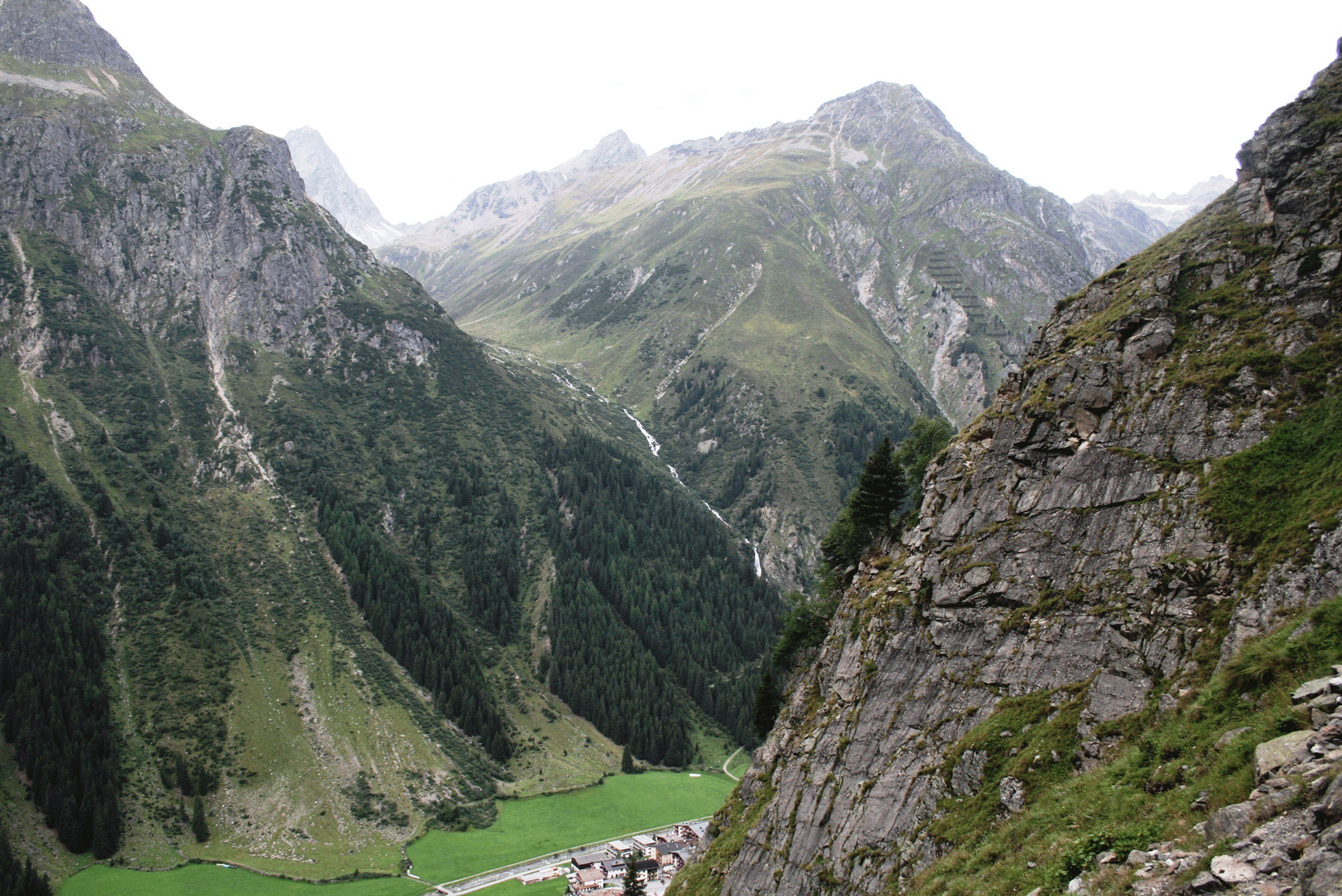
The Pitztal, situated in the south-western Austrian province of Tyrol, is a side valley of the Inn River. The longitudinal inner Pitztal (Figs. 1 and 2; TIRIS, 2015) features a narrow valley bottom with steep hillslopes. The study area (approximately encompassing the inner Pitztal) is about 20 km long in its north-eastern extension, with an average width of 6.5 km, covering an area of 133 km2. Only 25 % of the study area is forested, while 35 % is covered by pasture or natural grassland, and the remaining 40 % are sparse vegetation, bare rocks or glaciers (glaciers 2.5 %) (CORINE Land cover, 2016a, b, c). Elevation ranges from 1093 m a.s.l. at flow gauge Ritzenried up to 3340 m a.s.l. at the mountain ridge. The Pitztal is part of the Ötztal–Stubai crystalline and mainly consists of paragneiss and orthogneiss rocks mostly overlain by sandy Podzols.
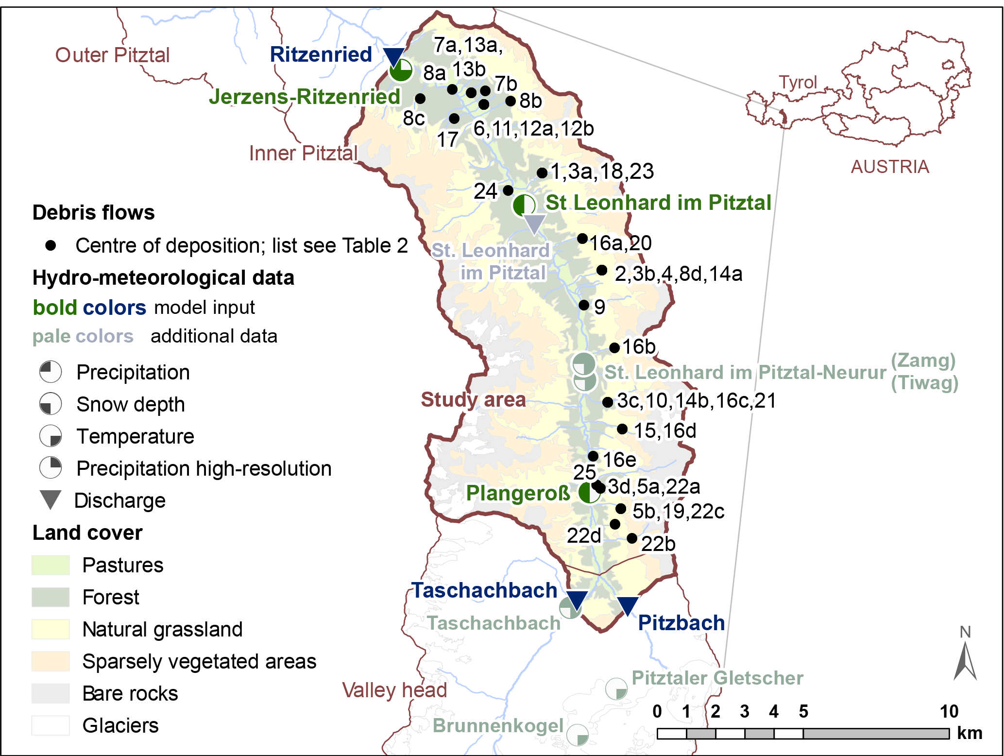
Figure 1Study area with locations of observed debris flows (centre of deposition), location of stream gauges and weather stations (debris flows: BMLFUW; gauging stations: TIWAG; weather stations: HD Tirol, TIWAG, ZAMG; land cover data: CORINE Land cover; glacier data: Austrian Glacier Inventory; rivers and location of catchment: TIRIS).
Mean annual precipitation in the inner Pitztal is about 1330 mm a−1, of which – on average – 42 % fall as snow. The inner-Alpine dry valley ranks among the driest regions of the Austrian Alps as it is located in the rain shadow of the Northern Limestone Alps and the main Alpine ridge. Mean yearly runoff totals ca. 930 mm a−1 (runoff coefficient: 0.7), displaying a nivo-glacial regime with the highest flows in June (river regime definition following Mader et al., 1996).
2.2 Data
Available hydro-meteorological data included daily time series of precipitation (P), mean temperature (Tmean) and potential evapotranspiration (Ep) for the period 1952–2012 as model input, while daily streamflow data (Q) for the period 1986–2013 were available for model calibration and validation (Fig. 3). The data were provided by national hydrological and meteorological services (HD Tirol, 2015, ZAMG, 2015) and a hydropower plant operator (TIWAG, 2015). Supplementing the daily precipitation sums, 15 min precipitation totals were available for stations St. Leonhard im Pitztal-Neurur (TIWAG) and Taschachbach from 1987 and 10 min totals for station St. Leonhard im Pitztal-Neurur (ZAMG) from 2007 onwards. These high-frequency data were in the following used as supporting information to interpret dominant debris flow triggers. The catchment outline and elevation zones for the semi-distributed model were obtained from a digital elevation model with 10 m resolution (Data.gv.at, 2016).
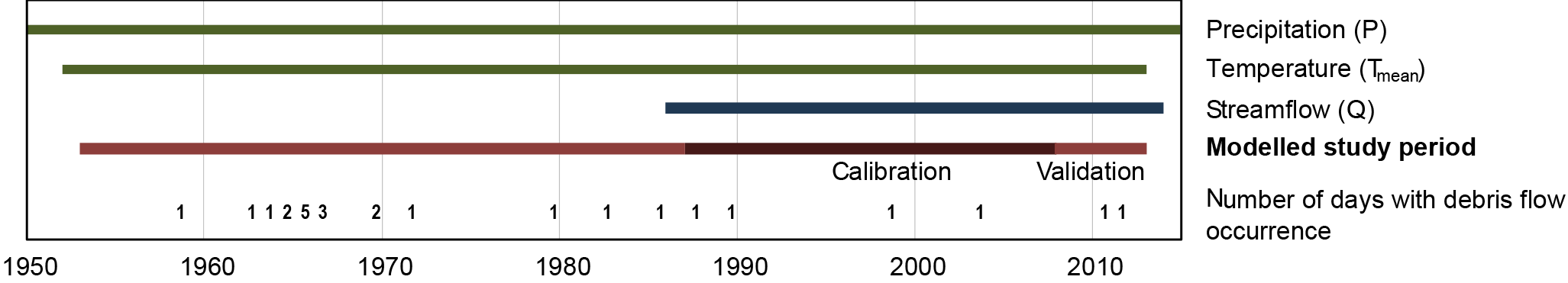
Figure 3Data availability, modelled study period and number of days with known debris flow occurrence. Only those debris flow events are plotted of which the exact date of occurrence was known, i.e. which were used for this study.
The daily precipitation input was calculated as the weighted mean of the stations Jerzens-Ritzenried, St. Leonhard im Pitztal and Plangeroß and – as all stations are located at the valley bottoms – was adjusted for elevation (Valéry et al., 2010; Beven, 2012), using high-resolution gridded vertical precipitation gradients provided by Mergili and Kerschner (2015) for the study area. The temperature data were, likewise, elevation corrected using an environmental lapse rate determined in relation to the nearby climate station Innsbruck Flugplatz (ZAMG, 2015; cf. Auer et al., 2007). For the estimation of the potential evapotranspiration, the Hargreaves and Samani (1985) equation was applied.
We restricted the hydrological modelling to the relevant study area, specifically adapting the hydrological model to the geomorphologically homogeneous inner Pitztal. We thereby avoided the need to model the extensively glaciated valley head and the outer Pitztal, where no significant debris flow activity was recorded. To do so, daily discharge data from the stations Pitz- & Taschachbach, located at the upstream boundary of the study area, were used as additional inflow to the model (Fig. 1). In contrast, daily discharge data from flow gauge Ritzenried at the catchment outlet were used for model calibration and validation. At the stations Pitz- & Taschachbach flow is measured in an artificial structure, providing very reliable data. The discharge data from the downstream gauge at Ritzenried were plausibility-checked against additional data from station St. Leonhard im Pitztal.
In addition, daily snow depth measurements for the whole study period 1953–2012 were available from stations Jerzens-Ritzenried, St. Leonhard im Pitztal and Plangeroß. Annual glacier extent data were obtained from the Austrian Glacier Inventory (2016) (Lambrecht and Kuhn, 2007), while annual glacier melt time series from three glaciers in the adjacent Ötztal catchment were accessible for the whole study period (Hintereisferner, Kesselwandferner), or from 1965 (Vernagtferner) from the WGMS (2017).
Within the study period, 1953–2012, 81 debris flow events in the inner Pitztal have been documented by the Austrian Federal Ministry of Agriculture, Forestry, Environment and Water Management (BMLFUW, 2015; cf. Hübl et al., 2008). For 43 debris flows (Fig. 1) occurring on 25 individual event days (hereafter referred to as “events”) the date of occurrence was known (Fig. 3) and could thus be used for the detailed analysis of the trigger conditions in this study. For the statistical assessment of debris flow occurrence, however, the full set of 81 debris flow events, i.e. also including those for which only the year or month of occurrence was known, was taken into account.
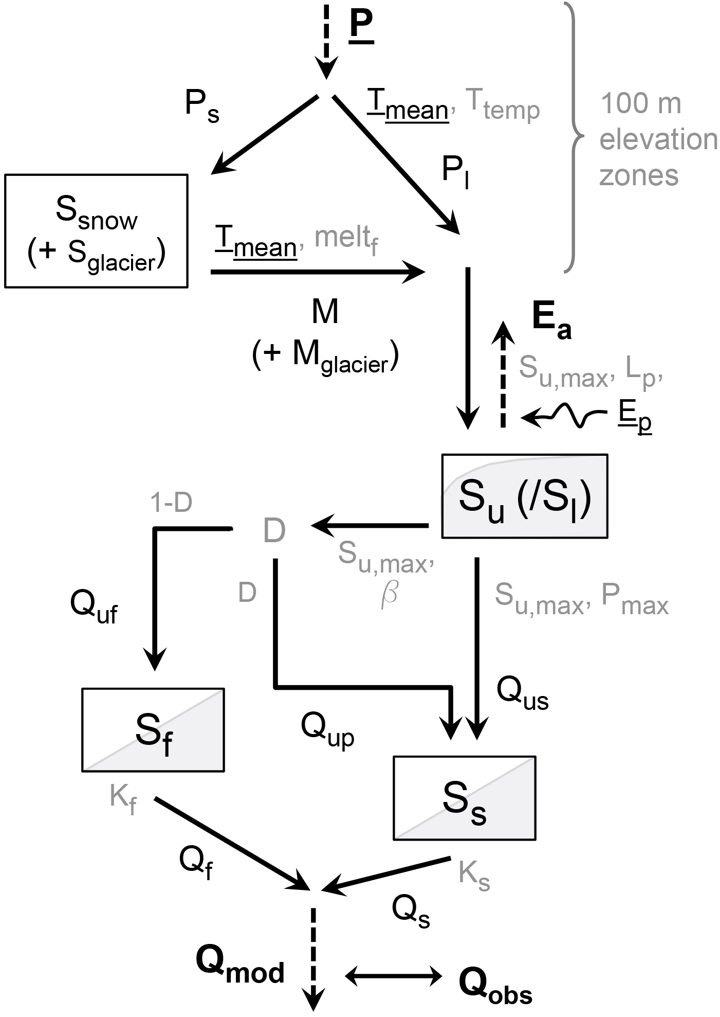
Figure 4Structure of the semi-distributed (stratification into 100 m elevation zones) hydrological model. Black symbols indicate fluxes and states, black underlined symbols indicate model input, and grey symbols indicate model parameters (for abbreviations, see Table 1).
3.1 The hydrological model
To estimate otherwise unavailable hydrological state and flux variables at the time of debris flow occurrences, we implemented a semi-distributed conceptual rainfall–runoff model on a daily basis.
3.1.1 Model structure
Adopting a flexible modelling strategy (Clark et al., 2011; Fenicia et al., 2011), which has proven highly valuable for many studies worldwide in the past (e.g. Leavesley et al., 1996; Wagener et al., 2001; Clark et al., 2008; Fenicia et al., 2014, 2016; Gharari et al., 2014; Hrachowitz et al., 2014), we customized and extensively tested a range of functionally different model structures and parameterizations (not shown). The most suitable of these tested model structures, which was subsequently used for the study catchment (Fig. 4), has nine free calibration parameters (Table 1b) and resembles the wide-spread HBV type of models, which were previously successfully applied over a wide range of environmental conditions (e.g. Seibert, 1999; Seibert and Beven, 2009; Fenicia et al., 2014; Berghuijs et al., 2014; Birkel et al., 2015; Hrachowitz et al., 2015; Nijzink et al., 2016b). All model equations are provided in Table S1 in the Supplement.
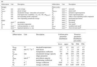
Table 1(a) Model storages and fluxes and (b) model calibration parameters with their uniform prior parameter distributions and the median as well as the 5–95th percentiles of the posterior parameter distributions of the set of behavioural solutions (for the model structure, see Fig. 4).
Briefly, the model was implemented with a semi-distributed snow routine, stratified into 100 m elevation zones. In the absence of more detailed data, the volume of water falling as snow (i.e. solid precipitation Ps) and eventually stored in the snowpack (Ssnow) was based on a simple temperature threshold method (e.g. Gao et al., 2017). Due to their minor importance in the snowmelt-dominated study catchment (Böhm et al., 2007) and in spite of their potentially distinct accumulation and ablation dynamics, glaciers were included in the snow module by allowing continued release of meltwater (Mglacier) after the depletion of the transient annual snowpack at elevations with observed perennial glaciers.
Rain (i.e. liquid precipitation Pl) and meltwater M (areally weighted sum from all elevation zones) directly enter the unsaturated root zone (Su), where a runoff coefficient (Cr) controls the proportion of incoming water directly released as preferential percolation (Qup) to the slow responding groundwater storage (Ss) or as influx (Quf) to a fast responding model component (Sf) and the proportion transiently stored as soil moisture in Su. Water can then leave Su either through an evaporative flux (Ea), comprising plant transpiration and evaporation, or through percolation (Qus) that eventually recharges the groundwater storage Ss. Streamflow is then generated from the combined outflow of Sf and Ss, both implemented as linear reservoirs with storage coefficients Kf and Ks, respectively.
The model at hand thus consists of a semi-distributed, elevation-stratified snow routine and a lumped hillslope component. While we tested different levels of spatial distribution due to different hydrological response units, including for example a parallel wetland component, we decided to go for the most parsimonious feasible model architecture, since more complex models neither improved model performance nor notably influenced the runoff behaviour. As flow velocities are very high, due to the elevated elevation gradients, and flow distances are relatively short, channel routing was considered negligible on the timescale of the implementation. Similarly, interception was neglected due to the limited amount of forested areas.
3.1.2 Model calibration and validation
Model calibration, based on Monte Carlo sampling with 106 realizations from uniform prior parameter distributions (Table 1), was performed for 1987–2007. For a robust model that can reproduce several aspects of the hydrological response simultaneously, thereby ensuring consistency of the internal processes (e.g. Gupta et al., 2008; Euser et al., 2013; Hrachowitz and Clark, 2017), a multi-objective calibration approach was applied. This was done by combining three objective functions, i.e. the Nash–Sutcliffe efficiencies (Nash and Sutcliffe, 1970) of flow (ENS,Q) and the logarithm of flow (ENS,log(Q)) as well as the volume error of flow (VE,Q; Criss and Winston, 2008) into the Euclidean distance DE to the “perfect” model as an overall objective function (e.g. Schoups et al., 2005; Hrachowitz et al., 2014; Fovet et al., 2015; Nijzink et al., 2016a):
In the absence of more detailed information, all three objective functions in DE were given equal weights. Note that in contrast to the three individual objective criteria, DE= 0 indicates a perfect fit.
The best performing 0.1 % of parameter sets in terms of DE, roughly corresponding to a performance threshold of 0.75 for each of the three individual performance metrics (see results section), were retained as behavioural solutions. These solutions were subsequently used to construct ensemble solutions and thus envelopes for the modelled variables, reflecting their respective sensitivities to parameter uncertainty.
The period 2007–2012 was thereafter used for post-calibration model testing and evaluation (“validation”; Fig. 3), based on the set of retained solutions and their performance metrics DE for that period. In addition, for a post-calibration plausibility check and evaluation of the snow routine at low elevations, we compared the timing of the presence of an observed snowpack (snow present yes/no) at the three climate stations with the modelled timing of the presence of snow storage at corresponding elevations in the model. Note that in the absence of time series of snow density, no more detailed evaluation could be done. For higher elevations we correlated the modelled annual glacier melt dynamics with the annual glacier melt time series from the three glaciers in the adjacent Ötztal valley.
3.2 Debris flow initiation analysis
To identify potentially different triggers for debris flow initiation, we then explored a range of hydro-meteorological system variables at days t when debris flows occurred. These included observed variables, such as daily precipitation P(t) (mm d−1), daily runoff Qobs(t) (mm d−1) and daily maximum temperature Tmax (∘C), as well as modelled state and flux variables such as unsaturated soil moisture Su(t) (mm) to account for antecedent moisture, daily snowmelt M(t) (mm d−1), daily runoff Qmod(t) (mm d−1) and the total liquid water present at the near surface, calculated as (mm), which is to be interpreted as an upper bound of near-surface storage as it does not consider drainage and evaporation at that time step.
For the observed system variables P (1953–2012) and Qobs (1986–2012), the analysis was based on the actual values recorded at the respective observation points for the day of occurring debris flows. Specifically, this involved the use of Qobs for each debris flow event measured at the gauge Ritzenried. For precipitation, the individual raw values recorded at the three weather stations Jerzens-Ritzenried, St. Leonhard im Pitztal and Plangeroß were used for the initial analysis to account for and illustrate the spatial variation in precipitation within the catchment. The subsequent estimation of debris flow probabilities (see below) was then based on the elevation-corrected, weighted areal mean precipitation. For temperature, the aerially weighted (according to elevations zones) temperature distributions as estimated from applying environmental lapse rates (see Sect. 2.2) were used.
The analysis of the modelled system variables was based on the behavioural parameter sets, which were used to generate distributions of values for each variable at the days of debris flow events occurring. The material presented hereafter is limited to M, Su, Sl, and Qmod. All other tested variables (not shown), such as groundwater storage, recharge, preferential flow or evaporative fluxes did not exhibit distinguishable patterns with respect to debris flow events; some of which may be attributed to poorly identifiable parameters and the resulting elevated uncertainty in these variables, i.e. the variation of the modelled variables generated with the suite of behavioural parameter sets was so high that for the same debris flow event this variable could take on either, a low or a high value, depending on which parameter set is considered (for examples see Supplement Fig. S1a–b). Note that the state variables Su and Sl were normalized and the analysis thus based on their respective relative water content. This allowed more insights as the model parameter representing the absolute storage capacity of Su, i.e. Su,max, varied within some range, which in turn is likely to mask relevant pattern (cf. Fig. S1c–d).
To be able to assess the variables' magnitude at debris flow initiation, we compared the magnitude of each system variable with the marginal distributions (i.e. distributions generated with the time series of all days, namely event days and non-event days; see also below) of the respective variables, allocating an “exceedance probability” to each value, rather than looking at the absolute numbers. Due to the generally very low occurrence probability of debris flow events and gaps in the data records (i.e. 25 well-documented events over 60 years), which potentially may in the following lead to instable and overly discontinuous statistical models, we limited the definition of exceedance probabilities (and all other probabilities estimated hereafter) to the period of the year in which all debris flow events occurred (“debris flow season”), i.e. from 15 May to 15 October 1953–2012. In other words, all probabilities reported hereafter are conditional on that period.
To facilitate a more objective and quantifiable comparison of the system variables, classes of exceedance probabilities were defined for the individual variables, with exceedance probabilities 1 ≥ Pe > 0.5 hereafter loosely referred to as high, 0.5 ≥ Pe > 0.1 as moderate, 0.1 ≥ Pe > 0.01 as low, and Pe ≤ 0.01 as very low, i.e. corresponding to extreme events and for precipitation to a lower bound of heavy precipitation events (cf. Schimpf, 1970). These classes of exceedance probabilities were subsequently used to systematically analyse if patterns of different dominant trigger mechanisms emerge from the observed and modelled data, i.e. daily precipitation P as a proxy of short duration, high intensity moisture input to the system, snowmelt M and Su as a metric of longer duration, lower intensity moisture input to the system, under different hydrological conditions. Due to the unavailability of historical sub-daily precipitation totals before 1987, the daily precipitation P was here used for the overall analysis as a proxy for precipitation intensities. Here the Pe < 0.01, equivalent to P= 45 mm d−1, implies a lowest physically possible limit for precipitation intensity of approximately 1.9 mm h−1, (i.e. during at least 1 h of that day a precipitation intensity of 1.9 mm h−1 was reached or even exceeded) which is consistent with the intensity thresholds for 24 h rainfall that were observed to trigger shallow landslides and debris flows in mountain areas as reported by Guzzetti et al. (2008). The high-resolution precipitation data (available from 1987 onwards; see Sect. 2.2) allowed, at least to some degree, a plausibility check of the identification of observed high-intensity rainfalls based on daily rainfall records during that time period. Please note, however, that exact exceedance probabilities for high-resolution precipitation data could not be determined due to the limited time frame of high-resolution data availability. Thus we provide conservative estimates of minimum exceedance probabilities.
Using the exceedance probabilities of the three system variables daily precipitation P, daily snowmelt M and relative soil moisture Su at the days when debris flows occurred then allowed, together with a qualitative consideration of the total liquid water availability Sl, daily runoff Qmod (and Qobs) and daily maximum temperature Tmax (as an indicator of the likelihood of a local convective rainfall event), a relative assessment of which variable contributed most to triggering an event and how the relative influences of the three individual variables varied over time, depending on the prevailing meteorological conditions. On days when a specific variable reached values that correspond to a high exceedance probability (1 ≥ Pe > 0.5; see above), the relative contribution of this variable to triggering debris flows was classified as having low relevance, while on days with moderate (0.5 ≥ Pe > 0.1), low (0.1 ≥ Pe > 0.01) or very low (Pe≤0.01) exceedance probabilities, the relative contributions of this variable to trigger debris flows were correspondingly classified as having moderate, high and very high relevance.
By comparing the values reached at debris flow initiation with the marginal distribution of the variables we applied a probabilistic concept (cf. Berti et al., 2012), which does not only consider the days where debris flows were reported, but also the non-event days. This, in turn, allowed an assessment of whether the respective variables were significantly increased, and thus likely to be (partially) responsible for the debris flow triggering. Please note that we on purpose do not provide any explicit posterior probabilities for debris flows in our main analysis, due to the limited sample size and the focus of the paper not being on providing probabilities o debris flow occurrence (and thus a blueprint for a prediction model), but to analyse the event's triggering conditions.
4.1 Hydrological model
The retained behavioural parameter sets (see posterior parameter distributions in Table 1) generated model outputs that reproduced the features of the hydrological response in a generally plausible way, as can be seen in Fig. 5 for some selected years and in Fig. S2 for the remaining years of the study period. This is on the one hand reflected in the rather elevated performance metrics for streamflow. The models' best fit overall objective function reached DE= 0.25 for the 20-year calibration period, with 0.85, 0.93, and 0.81. The model similarly produced adequate performance levels for the validation period with DE= 0.26 (5∕95th percentiles 0.25 ≤ DE≤ 0.31), 0.86 (0.82 ≤ 0.87), 0.93 (0.91 ≤ 0.93) and 0.79 (0.76 ≤ 0.80). On the other hand, post-calibration evaluation (cf. Hrachowitz et al., 2014) also indicated that the overall pattern in snow and glacier dynamics, which the model was not trained for, were adequately captured. Comparing the information on whether snow has been present (yes/no) at the three climate stations Jerzens-Ritzenried, St. Leonhard im Pitztal and Plangeroß with the model's results at corresponding elevations shows that the (non-)presence of snow corresponds reasonably well, with correlation coefficients reaching r= 0.77, 0.87 and 0.88, respectively (with p < 0.001 throughout), for the best model fit. Likewise, the observed glacier melt dynamics correlated well with the modelled snowmelt dynamics at higher elevations with the best fit model's correlation coefficients r= 0.85, 0.81 and 0.91 (p < 0.001 throughout) for the Hintereisferner, the Kesselwandferner and the Vernagtferner, respectively.
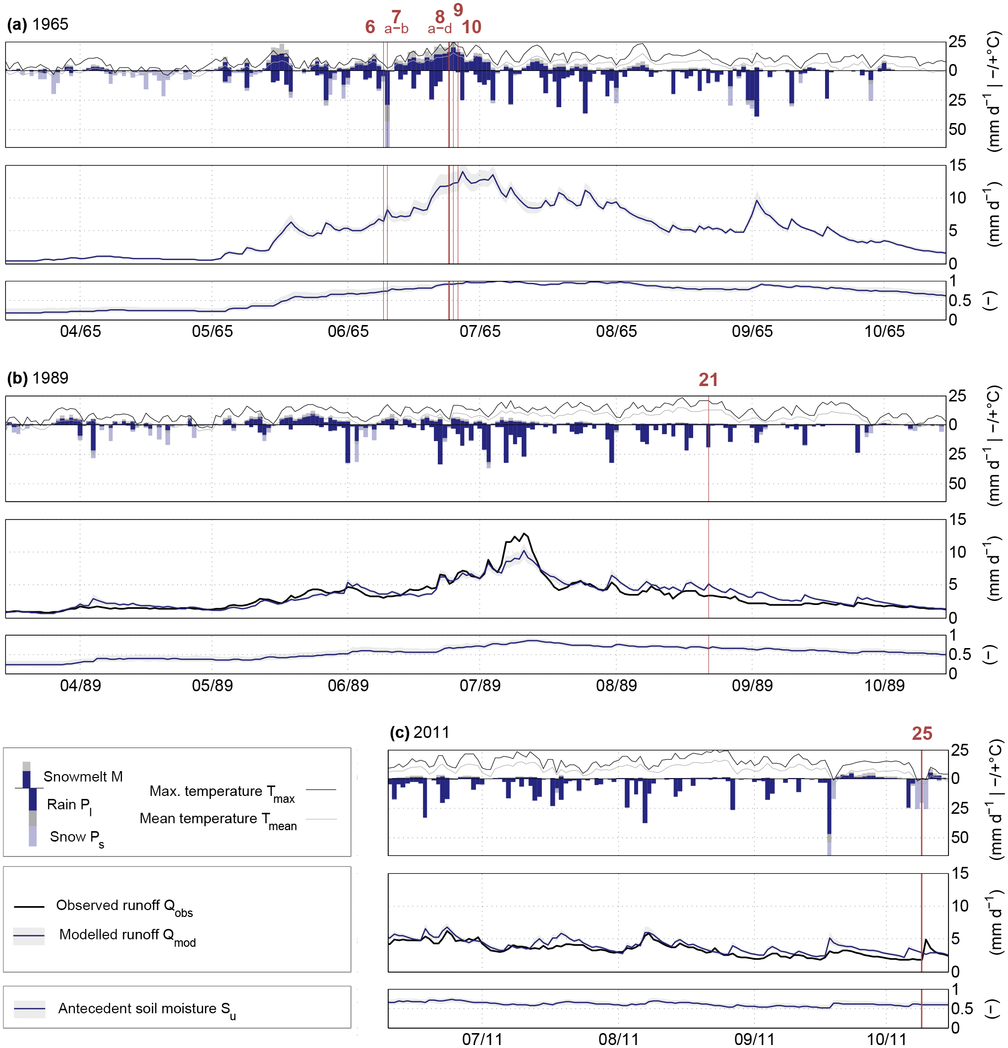
Figure 5Observed daily streamflow Qobs (black solid line), daily mean temperature Tmean at mean elevation (grey solid line) and maximum temperature Tmax at mean elevation (black solid line) as well as, based on observed precipitation data, modelled daily rainfall Pl (dark blue downward columns for the 5th percentile, including grey downward columns for the 95th percentile), daily snowfall Ps (light blue downward columns for the 5th percentile, including grey downward columns for the 95th percentile) and daily snowmelt M (dark blue upward columns for the 5th percentile, including grey upward columns for the 95th percentile), modelled streamflow (dark blue line for the median and the grey shaded area for the 5∕95th percentiles of all behavioural model solutions) and modelled relative soil moisture (solid blue line for the median and the grey shaded area for the 5∕95th percentiles) for the 3 selected years (a) 1965, (b) 1989 and (c) 2011 (all remaining years with debris flow occurrence are provided in Fig. S1). The days where a debris flow event has been documented are marked with red vertical lines. Please note that the plots display the period 15 March to 15 October to depict the start and amount of rainfall and snowmelt; however, the analysis (Figs. 6 and 7) is based on the period 15 May to 15 October.
4.2 System variables at debris flow initiation
In the following the values of hydro-meteorological variables at the days of debris flow occurrences were extracted from the observed and modelled time series. On 3 out of the 25 days with debris flows (nos. 7, 11, 19), the observed precipitation at all three rain gauges exceeded P= 45 mm d−1, corresponding to a precipitation exceedance probability Pe= 0.01 over the study period (Fig. 6a). This threshold was exceeded for at least one gauge on 2 further event days (nos. 21, 24). In addition, precipitation recorded at all three gauges reached exceedance probabilities 0.01 < Pe≤ 0.1 (∼ 17 mm d−1) for 3 event days (nos. 1, 16, 22) and for at least one gauge on 4 days (nos. 3, 12, 23, 25). On 9 more event days precipitation with 0.1 < Pe≤ 0.5 was recorded for at least one gauge, while on 4 days (nos. 2, 8, 9, 20) no precipitation was observed at any gauge.
High modelled snowmelt rates with Pe≤ 0.01 for almost all behavioural solutions, corresponding to M= 15 mm d−1, occurred on 4 event days (nos. 8, 9, 10, and 17; Fig. 6c), while snowmelt plotted between 0.01 < Pe≤ 0.1 for one event (no. 20). All remaining events, except for no. 25, for which no snowmelt was generated by the model, occurred on days with at least some degree of snowmelt.
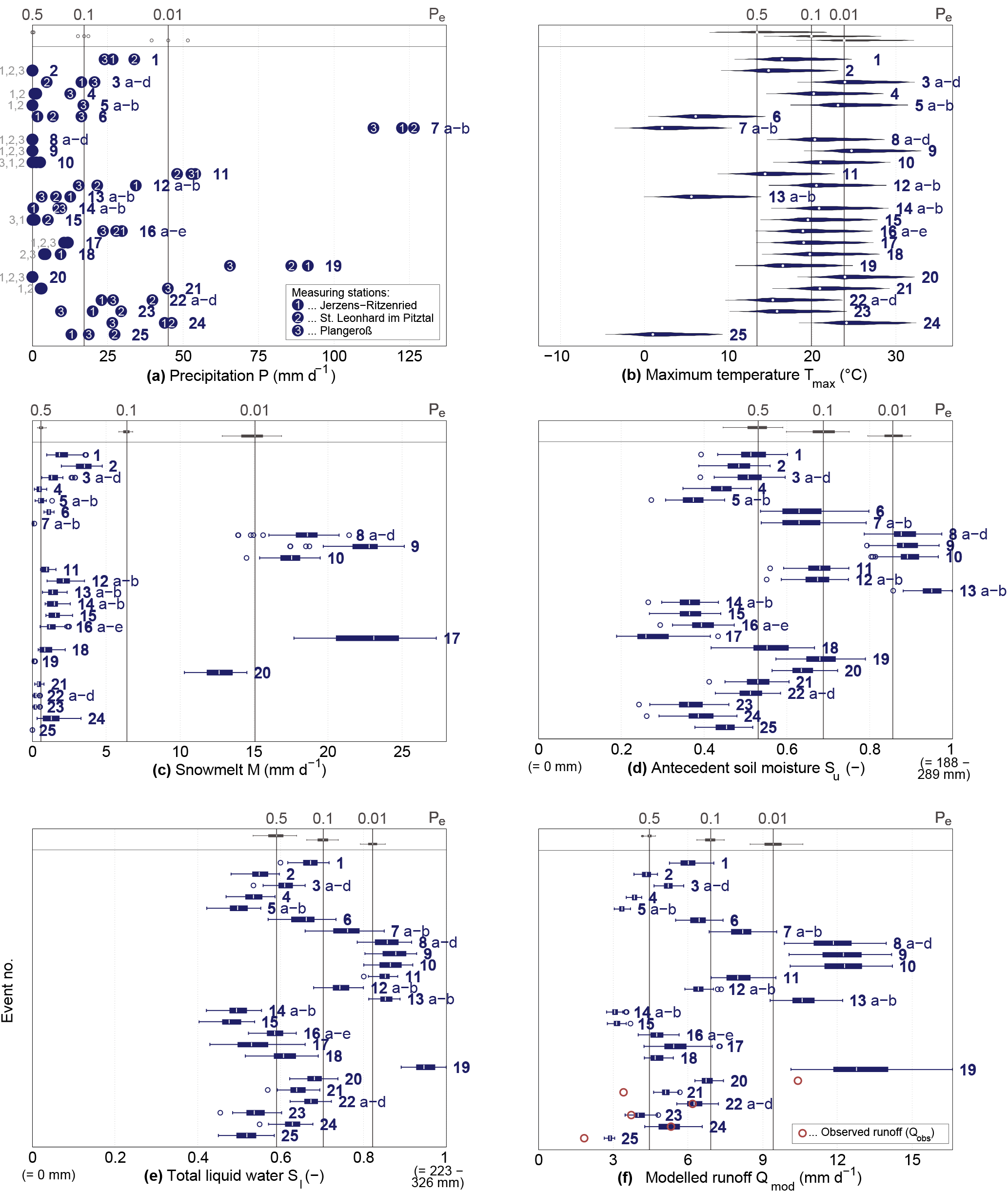
Figure 6Plots of relevant system variables: (a) precipitation P elevation adjusted for mean catchment elevation, (b) maximum temperature Tmax for all catchment elevations (blue bars) and mean elevation (white dots), and (c–f) modelled snowmelt M, antecedent soil moisture Su, total liquid water availability Sl, and runoff Qmod (and, where available, Qobs). Boxplots comprise all behavioural models. For event numbering see Table 2. Pe is the observed/modelled probability of exceedance (i.e. marginal distribution; see Sect. 3.2) for a specific variable considering all days between 15 May and 15 October within the study period 1953–2012.
Similarly, the mean modelled antecedent soil moisture Su (Fig. 6d) from behavioural parameter sets was exceptionally high on 4 event days (nos. 8, 9, 10, and 13), i.e. at each event day at least 75 % of the behavioural solutions indicate Pe≤ 0.01, and at least moderately elevated on at least 7 additional days (nos. 6, 7, 11, 12, 18, 19, and 20). For completeness and as support for the following analysis, the maximum daily temperature (Tmax) distribution over all elevation zones in the catchment (Fig. 6b), the near-surface total liquid water storage Sl (Fig. 6e), the observed and modelled runoff Qobs and Qmod (Fig. 6f), respectively, are also shown. While Sl, Qobs and Qmod broadly reflect the combined pattern of P, M and Su, the pattern of Tmax suggests that almost 50 % of the events (11 out of 25) occurred on days with high or very high temperatures (i.e. Pe < 0.1).
4.3 Dominant debris flow triggers
The exceedance probabilities presented above of several system variables at days of debris flow occurrence allowed us to estimate the changing relative relevance of P, M and Su, respectively, for triggering the observed debris flows on the 25 event days and to classify the debris flows according to the variable that is the most relevant (i.e. “dominant”) contributor for triggering debris flows on the individual event days (Table 2).
4.3.1 The role of high-intensity precipitation
On the 3 event days with precipitation totals of P > 45 mm d−1 observed at all three stations and thus Pe ≤ 0.01 (nos. 7, 11, and 19), being a lower limit of traditional rainfall intensity-duration thresholds for debris flow initiation (see above; Guzzetti et al., 2008), this heavy (cf. Schimpf, 1970) although not necessarily high-intensity and short-duration convective rainfall is very likely to have a very high relevance as a contributor to initiating the debris flows (Table 2). The values of Su for these events, with exceedance probabilities Pe ≤ 0.25, suggest some moderately relevant additional contributions from previous water input that left the soil at above-average moisture conditions. Although present at these event days, snowmelt is likely to have low relevance (Pe ≥ 0.40) as a contributor to these debris flow events. Interestingly, while temperatures have been moderate (0.1 < Pe≤ 0.5) for nos. 11 and 19, they have been rather low for event no. 7 (Figs. 5a and 6b). Thus, for this event, the precipitation only fell as rain at lower elevations (< 2000 m a.s.l.) and the debris flows are therefore likely to have been initiated at lower elevations, which is in accordance with the associated observation of these debris flows, located at the lowest section of the inner Pitztal (Fig. 1).
For event nos. 21 and 24, heavy precipitation was likely to have a very high relevance as a contributor to triggering debris flows, as well (Table 2). This is in spite of the catchment average observed precipitation on these days being less extreme, with 0.01 < Pe≤ 0.1. Rather, as shown in Fig. 6a, both debris flows occurred close to the rain gauge, with the respective highest precipitation recorded on that day, i.e. station Plangeroß for no. 21 and St. Leonhard im Pitztal for no. 24 (Fig. 1), both of which reached Pe≤ 0.01. Together with the high temperatures (Fig. 6b), this suggests that the precipitation on these days very likely occurred as highly localized and temporally concentrated convective rainstorms (“thunderstorms”), which potentially exhibited precipitation intensities far above the ∼ 1.9 mm h−1 threshold (as derived as the lower limit from the observed 45 mm d−1 if precipitation is uniformly distributed over 1 day) for debris flow initiation in mountain areas (Guzzetti et al., 2008), at these two stations. In fact, the available high-resolution precipitation data show that exceptionally high maximum intensities (6.3 mm 15 min−1 and 10.8 mm 10 min−1, corresponding to exceedance probabilities of Pe < 0.0001) occurred on these 2 days. Snowmelt had some moderate additional contribution to event no. 24, while its relevance was low for no. 21 (Fig. 6c). Similarly, the largely below-average Su indicates a low relevance of antecedent soil moisture for these two events (Fig. 6d). A similar reasoning applies to event nos. 3 and 12, albeit somewhat less unambiguously (Table 2). For both events, catchment averaged observed precipitation fell within exceedance probabilities 0.01 < Pe≤ 0.1, and thus below the empirical trigger threshold. However, also in this case, the rain stations recording the highest daily precipitation totals were largely the ones closest to the observed debris flows, i.e. Plangeroß for no. 3 and Jerzens-Ritzenried for no. 12 (Fig. 1). Although the precipitation recorded at these stations for the 2 event days did not reach the Pe≤ 0.01 threshold (Fig. 6a), the high to very high temperatures on these days plausibly suggest the presence of convective precipitation cells and thus of temporally and spatially concentrated and thus high-intensity rainfall. In contrast, while the temperatures for event nos. 1, 16, 22 and 23 were only somewhat above average, the precipitation recorded at gauges close to the respective events (Fig. 1) was mostly closer to the threshold Pe= 0.01 than for event nos. 3 and 12 discussed above (Fig. 6a), implying that a moderate temporal concentration of these values to precipitation durations ≤ 12 h (and thus not necessarily convective) on the respective event days would already result in precipitation intensities exceeding the threshold for debris flow initiation. Again, for nos. 22 and 23 the high-resolution precipitation intensity data show that clear intensity peaks have occurred (Table 2). Conversely, only rather moderate precipitation (0.1 < Pe≤ 0.5), for both the catchment average and the gauge with the respective highest recorded values, was observed for event nos. 4, 5 and 14, albeit most of them with the highest values for the gauges closest to the debris flows. The high temperatures (Pe≤ 0.1) indicate that localized and temporally highly concentrated precipitation from convective events and above the necessary trigger thresholds is not unlikely for these days. Similarly and although the precipitation data do not give any direct evidence, the merely moderate snowmelt and antecedent soil moisture together with maximum temperatures nearly reaching the Pe < 0.1 threshold for event nos. 15 and 18 suggest that highly localized (and thus potentially not adequately recorded) and/or temporally concentrated precipitation may have generated sufficient local precipitation intensities to trigger these debris flows, as well. Lastly, elevated precipitation values (0.01 < Pe≤ 0.1) were observed for event no. 25, therefore suggesting triggering by precipitation, even though temperatures have been – atypically – very low (Pe= 0.99, corresponding to maximum temperatures of −5 to +7 ∘C (Fig. 6b)). This interpretation is supported by the available high-resolution precipitation data (Pe < 0.01). Please note that the output from the hydrological model suggests that all of the precipitation has fallen as snow (and would therefore not be likely to trigger any debris flow at all); however, this is due to the mean temperature amounting to −3.8 ∘C and an inherent limitation of using a daily averaged temperature input. The above points suggest, together with the generally low antecedent moisture storage Su from preceding and potentially more persistent rain and snowmelt (Fig. 6d), that very intense, relatively short-duration precipitation was likely a highly relevant contributor to event nos. 1, 3, 4, 5, 12, 14, 15, 16, 18, 22, 23, and 25, although the level to which this assessment is fully warranted by the available data varies between the events. In addition, debris flow initiation was supported by contributions of snowmelt (nos. 1, 3, 12, 14, 15, 16, and 18; Fig. 6c) for several events. However, as most of the above events occurred during summer (i.e. July and August) after the snowmelt peaks, which typically occur much earlier in the season (i.e. May and June; see Figs. 5 and S2) and thus when only relatively little snow was left, the snowmelt contributions to these events remained quite moderate.
Table 2The 25 recorded debris flow events in the inner Pitztal that occurred at known dates since 1953. For each event the exceedance probabilities Pe associated with the observed variables daily precipitation P, daily maximum temperature Tmax and daily mean streamflow Qobs as well as with the modelled variables daily snowmelt M, daily antecedent moisture content Su, daily total near-surface water availability Sl and the daily streamflow Qmod at the day of the respective events are given. Bold and italic values indicate a very high relevance (Pe≤ 0.01) and bold values a high relevance (0.01 < Pe≤ 0.1) of each individual variable for a given event; normal values indicate moderate relevance (0.1 < Pe≤ 0.5) and italic values indicate a low relevance (Pe > 0.5). The columns indicating the relevance of contributing variables show the likely level of importance of the three variables that directly affect debris flow initiation (P, M, Su), after consideration of supporting evidence from variables, such as Tmax, that do not directly affect the triggering of debris flows. As an additional plausibility check of our interpretation, information on high-resolution precipitation data is provided (column when available. The direct support by the data column indicates to which extent the classification of the contributing variables into very high/high, moderate and low is directly supported by daily data (: excellent support, +: strong support, ∼: moderate support), and thus provides an indicative quality check of how likely this interpretation is to reflect the real conditions during debris flow initiation.
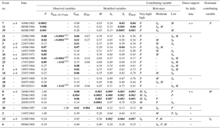
(21) Taschachbach: 6.3 mm 15 min−1 (St. Leonhard im Pitztal-Neurur (TIWAG): 0.7 mm 15 min−1). (24) St. Leonhard im Pitztal-Neurur (ZAMG): 10.8 mm 10 min−1 (St. Leonhard im Pitztal-Neurur (TIWAG): 5.2 mm 15 min−1; Taschachbach: 2.1 mm 15 min−1). (22) Taschachbach: 6.4 mm 15 min−1 (St. Leonhard im Pitztal-Neurur (TIWAG): 0 mm). (23) St. Leonhard im Pitztal-Neurur (TIWAG): 0.9 mm 15 min−1 (Taschachbach: 0.4 mm 15 min−1). (25) St. Leonhard im Pitztal-Neurur (ZAMG): 0.9 mm 10 min−1 (St. Leonhard im Pitztal-Neurur (TIWAG): 0.5 mm 15 min−1; Taschachbach: 0.5 mm 15 min−1).
4.3.2 The role of snowmelt
Event nos. 8, 9 and 10 occurred on days when the modelled snowmelt reached exceedance probabilities of Pe≤ 0.01 (Fig. 6c, Table 2) and only very little to no additional precipitation was recorded. In spite of these exceedance probabilities, the total median melt volumes of about 18–23 mm d−1 on these days, equivalent to melt intensities of 0.75–0.96 mm h−1 for uniform 24 h melt, fall short of the debris flow initiation threshold for precipitation intensities of ∼ 1.9 mm h−1. However, and importantly, it is very likely that the required intensity threshold was exceeded locally. The reasons are that on the one hand most of the meltwater on the event days was generated at high elevations (> 2000 m), leading to locally considerably elevated melt rates and thus intensities at these higher elevations (up to 38 mm d−1 for nos. 8 and 10 and up to 46 mm d−1 for no. 9), which are the source area of debris flows. On the other hand, melt is unlikely to occur uniformly over a 24 h period. This causes further temporal concentrations of meltwater generation, and thus higher peak melt intensities within individual days which will roughly reflect daily temperature variations, yet in an attenuated, temporally lagged manner due to the thermal capacity of the snowpack. Based on the above reasoning, the snowmelt contribution is thus likely to have a very high relevance for the initiation of debris flows on these event days (Table 2). In addition, antecedent soil moisture was also at very high levels, i.e. Pe≤ 0.01 (Fig. 6d). This continuous build-up of antecedent soil moisture by persistent snowmelt and some moderate rainwater input over the preceding days (Fig. 5a), resulting in catchment-wide almost fully saturated conditions, is thus also likely to provide highly relevant contributions to trigger the debris flow event nos. 8, 9, and 10. Indeed, total liquid water availability and also modelled runoff have been at least as high (Pe≤ 0.003) as those of event nos. 7, 11, and 19, which have been identified as triggered by heavy precipitation with a high confidence (Sect. 3.2.1, Table 2). In contrast, the precipitation totals observed on the 3 days exceed Pe > 0.1, with no precipitation recorded at all for nos. 8 and 9. Although localized, high-intensity precipitation missed by the precipitation gauges cannot be ruled out for these event days, given the already high melt rates of up to 46 mm d−1 and the fact that for nos. 8, 9 and 10 most gauges did not observe any precipitation, rainfall is thus considered to make no more than a moderate additional contribution to the initiation of these debris flows.
For no. 17, an extremely low snowmelt exceedance probability of Pe= 0.0001 was estimated, resulting from the highest snowmelt rate that was modelled within the study period 1953–2012. Yet a maximum local melt intensity of “only” 38 mm d−1 has been calculated which equals those of event nos. 8 and 10, due to the snowmelt occurring over a wider range of elevations (> 1700 m a.s.l.) on that day. As at all three climate stations, moderate (0.1 < Pe≤ 0.5) precipitation was recorded, and rainfall will have played a more prominent role than for event nos. 8, 9 and 10, making this event a classical rain-on-snow triggered event (cf. Church and Miles, 1987).
Mirroring the reasoning for event nos. 8, 9 and 10, the snowmelt exceedance probabilities of 0.01 < Pe≤ 0.1 for event no. 20 and 0.1 < Pe≤ 0.5 for no. 2 suggest at least high and moderate snowmelt contributions, respectively, for triggering the associated debris flow. Interestingly, for both events, the snowmelt has been restricted to a smaller elevation band (> 2400 m a.s.l.) than for the other events described above, thus rendering higher local melt intensities. Indeed, for no. 20 maximum melt intensities of ca. 39 mm d−1, equalling those of event nos. 8, 10 and 17, were modelled, and for no. 2, maximum melt intensities of up to 16 mm d−1, which – given a catchment mean snowmelt of only 4 mm d−1 – are also quite noteworthy. Similarly, the absence of observed precipitation and – in case of no. 2 – only moderate maximum temperature, suggests that precipitation is likely to be of low relevance for the initiation of debris flow event nos. 2 and 20, although the occurrence of small convective shower cells cannot be fully dismissed. Note, however, that the direct evidence provided by data in particular for no. 2 is less strong than for event nos. 8, 9, 10 and 17, leaving the assessment of the relative relevance of the individual contributors less robust.
To sum up, event nos. 2, 8, 9, 10, 17, and 20 have been associated with snowmelt as the primary trigger, while the assumed additional influence of rainfall (i.e. “rain-on-snow”) and antecedent soil moisture varies between the events. Additional supporting evidence for the above reasoning is that the general timing of the above events coincides well with the snowmelt season. Snowmelt typically peaks during May and June in the study region (Figs. 5 and S2), while high-intensity, convective rainfall is mostly only observed later in the season (i.e. July and August).
4.3.3 The role of antecedent soil moisture
For event no. 13, the gradual build-up of soil moisture Su by considerable precipitation in the days before as well as by persistent, low-intensity snowmelt in the weeks before the event to nearly fully saturated levels (Fig. S2f), resulted in a soil moisture level with an exceedance probability of Pe≤ 0.01 (Fig. 6d, Table 2). This suggests that soil moisture had likely a very high relevance to trigger this event. Precipitation and snowmelt rates corresponding to 0.1 < Pe≤ 0.5 provided additional moderate contributions to initiate event no. 13.
A similar pattern can be found for event no. 6, albeit with a lower relative contribution from soil moisture, whose contribution to trigger the event was moderately relevant (Pe= 0.24), as were the contributions of precipitation (Pe= 0.19) and snowmelt (Pe= 0.40).
Interestingly, both events, nos. 6 and 13, occurred in the lowest part of the study area, where relatively large parts are vegetated (Fig. 1), while most of the events associated with high-intensity precipitation (nos. 1, 3, 4, 5, 12, 14, 15, 16, 18, 21, 22, 23, 24, and 25) took place at higher elevations. For these events, the antecedent soil moisture estimates have been mostly below average, which not only backs the interpretation of high-intensity precipitation as dominant trigger (as discussed in Sect. 4.3.1), but may also indicate that the antecedent soil moisture is in general of minor significance at higher elevations, as in it headwaters the catchment is dominated by lower-permeability surfaces (bare rock, sparsely vegetated areas) and shallow soils that only provide limited storage capacities (cf. Berti and Simoni, 2005; Coe et al., 2008; Gregoretti and Fontana, 2008).
4.3.4 Seasonally varying importance of the different trigger contributions
The above analysis illustrated quite clearly that water inputs originating from different individual “sources” can significantly contribute to generate trigger conditions in the study area. The data further suggest that the relative relevance of each these variables contributing to the actual trigger conditions does vary over time. Even more, there is some evidence that among the three tested variables, high-intensity and potentially short-duration precipitation P may be not the consistently most relevant (or “dominant”) contributing factor for all events. Rather, it is not unlikely that also high-intensity snowmelt M and similarly, although with some lower degree of confidence, persistent, lower intensity water input, building up antecedent soil moisture content Su and eventually causing saturated conditions, can generate the most relevant contributions to reach trigger conditions. More specifically, high-intensity precipitation was likely to be the dominant contributor to trigger debris flows on 17 out of 25 event days (68 %). This corroborates previous studies that this type of precipitation is the prevalent trigger in such environments (e.g. Berti et al., 1999; Marchi et al., 2002; Berti and Simoni, 2005; Coe et al., 2008; Gregoretti and Fontana, 2008; Braun and Kaitna, 2016; Ciavolella et al., 2016). In addition, however, high-intensity snowmelt was likely the dominant contributor on 6 days, corresponding to 24 % of the observed events and antecedent soil moisture on 2 event days (8 %), highlighting their critical individual contributions to debris flow initiation.
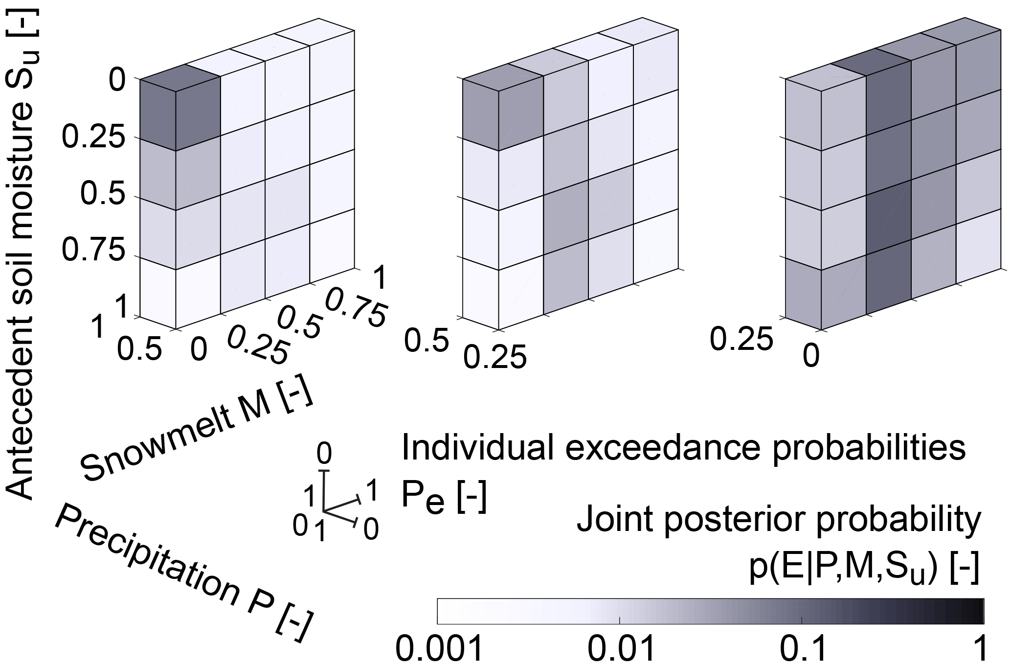
Figure 7Individual exceedance probabilities Pe of precipitation (P; x-axis), snowmelt (M; y-axis) and relative antecedent soil moisture (Su; z-axis) as well as the corresponding joint conditional posterior probabilities of an event occurring given specific values (expressed as classes of exceedance probabilities) of precipitation, snowmelt and antecedent soil moisture, ).
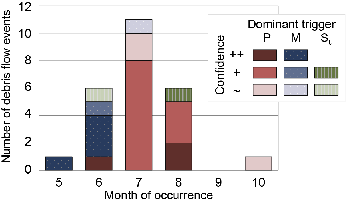
Figure 8Debris flow events by month of occurrence and likely dominant trigger; shades indicate the relative strength (the darker the stronger) of the dominant trigger in terms of (1) its relative relevance compared to the other contributing variables and (2) the extent to which it is directly supported by data (see also Table 2).
A somewhat different, more quantitative perspective is given by Fig. 7, showing the joint conditional posterior probabilities of a debris flow event E occurring, given the exceedance probability of each individual variable P, M and Su, i.e. . Note that ) is shown in classes of exceedance probabilities with an increment of 0.25 to allow a meaningful visualization of the clustering effects. High probabilities of debris flow events predominantly cluster at low exceedance probabilities of precipitation or in other words, on days with high precipitation totals which were exceeded only in 25 % of all days in the study period (i.e. the right-most slice in Fig. 7). Under such conditions, additional contributions from snowmelt or antecedent soil moisture are not necessarily required to trigger debris flows (e.g. Aleotti, 2004; Berti et al., 2012), which is also reflected in the elevated ) for low M and Su in that class of precipitation exceedance probability. However, elevated event probabilities can also occur when little to no precipitation is observed, i.e. at exceedance probabilities of P > 25 %, which is roughly equivalent to P < 6 mm d−1, but when instead higher melt rates and/or, albeit to a lesser extent, antecedent moisture levels are likely to be present, as suggested by the model results. Although both the relative proportions of the different dominant triggers as well as actual values of ) as shown in Fig. 7, may be subject to some change over time due to the relatively low absolute number of events with respect to the 60-year study period, the general pattern strongly underline the varying roles of the three variables under consideration as individual and potentially dominant contributors to debris flow trigger conditions in the study region.
Most debris flow events in the study area occur between mid- and late summer (Fig. 8), when spring precipitation and persistent snowmelt have developed above-average soil moisture levels and when the frequency of high-intensity, convective rain storms increases (Figs. 5 and S2). Further analysis also revealed a relatively clear pattern in the seasonally changing relative relevance of the three considered variables as contributors to debris flow trigger conditions. In general, three distinct seasonal debris flow trigger regimes emerge from the analysis, which to a high degree reflect both the seasonal cycle in the hydro-meteorological conditions and in debris flow occurrence, from snowmelt- to convective-rainfall-dominated debris flow triggers. While late spring and early summer events are mostly associated with snowmelt in combination with elevated soil moisture and only very minor contributions of high-intensity precipitation, the latter is, for the above reasons, the dominant trigger in summer and early autumn. While the former may be trivial given that significant snowmelt is less common from July onwards, it is interesting to observe that high-intensity precipitation may be, though also sometimes occurring in spring and early summer, less relevant for triggering debris flows at that time of the year. In our dataset, event no. 7 occurring in early June 1965 was attributed to high-intensity rainfall, while event nos. 8–10, occurring in the same month, were predominantly triggered by snowmelt, forming a clear exception to this general rule. Also, in the same month, triggering by elevated soil moisture conditions due to the combined effect of long-lasting rainfall and snowmelt has been observed (event no. 6). This shows how debris flow triggers can change very rapidly following weather changes. The general pattern (high-intensity precipitation in summer vs. snowmelt in spring as the dominant debris flow triggers) mostly arises from a combination of two factors, namely that in spring considerable proportions of precipitation observed at lower elevations (1) still fall as snow, in particular at higher elevations, and (2) are, if falling as rain, intercepted by, transiently stored in and/or potentially refrozen in the snowpack, in particular if the snowpack has not yet reached isothermal conditions at 0 ∘C throughout the region of interest. Although a mature snowpack later in the melt season may reverse the latter into a positive feedback, i.e. actually reinforcing intensive precipitation in rain-on-snow events (e.g. Harr, 1981; Conway and Raymond, 1993; Cohen et al., 2015), both factors above can, in principle, also cause an attenuation of the observed precipitation intensity as water will be released from the snowpack with some time lags and potentially over a longer time, i.e. at lower rates than the observed ones. The immediate implications are then that thresholds for debris flow initiation estimated from traditional rainfall (but also precipitation) intensity-duration approaches may be suitable for some regions, as for example demonstrated by Berti et al. (2012), who showed that antecedent soil moisture is of limited importance in their study region, but will be unreliable for certain hydrological conditions, in particular in snow dominated regions (cf. Decaulne et al., 2005), and thus insufficient for meaningful predictions of debris flows. As a step forward, it may therefore be beneficial to move towards understanding the problem in a more comprehensive and thus multivariate way, expressing and combining the varying relative relevance of different water “sources” in terms of total liquid water availability Sl (see Fig. 6e as an example) in the source zone of debris flows, as recently also emphasized by Bogaard and Greco (2018).
4.3.5 Discussion
We would like to reiterate here that, as in any hydrological study at scales larger than the hillslope scale, the issue of epistemic errors in data (Beven, 2012; Beven et al., 2017a, b), arising from the typically insufficient spatial but also temporal resolutions of the available observations (mostly precipitation) can introduce considerable uncertainty in the interpretation of a specific hydrological system (e.g. Valéry et al., 2010; Nikolopoulos et al., 2014; Marra et al., 2017) which is further exacerbated by complex, mountainous terrain (e.g. Hrachowitz and Weiler, 2011). This is in particular relevant for debris flows as they depend on the hydrological conditions at the specific location of their initiation, which is frequently of very limited spatial extent. Borga et al. (2014), for instance, reported the occurrence of several debris flows that were triggered by highly localized, high-intensity rainfall > 100 mm h−1, which remained completely unrecorded by rain gauges at a 5–10 km distance.
We also explicitly acknowledge additional uncertainties arising from the use of a simple, semi-distributed model to represent the hydrological system of the study area. Such models are clearly oversimplifications of the detailed processes controlling the storage and release of water. Together with the effect of the above discussed data errors, this explains, why the model cannot fully reproduce some of the features in the observed hydrograph (e.g. Figs. 5b, c and 6f), in spite of its adequate overall performance. Indeed, out of the 6 debris flow days, where both modelled and measured runoff values were available, the modelled runoff in three cases did not correspond particularly well to the measured runoff (Fig. 6f), although in those cases where the runoff was underestimated by the model (no. 20), this was most likely due to unrecorded or underrecorded precipitation. This ambiguity equally affects the estimates for total soil moisture, while the modelled snowmelt and the antecedent soil moisture, in contrast, can be assumed to be more correct, as these variables are integrations over time, in which case erroneous precipitation measurements are likely to be compensated and thus of less consequence (e.g. Hrachowitz and Weiler, 2011). In addition, the spatial integration of local processes is likely to result in a misrepresentation of hydrological conditions for the locations of debris flow initiation.
However, even though the model is rather simple with limited spatial differentiation, we would like to point out that our approach is not due to an ill-advised oversimplification. Rather, it is the (un-)available data that limit a meaningful spatial differentiation. The most crucial meteorological input, namely precipitation, is very often (and also here) not available on a spatially sufficiently distributed basis (see above), let alone for the actual source area of a specific debris flow. Furthermore, the calibration of a more distributed model would be more problematic and – in the case of fully distributed physically based models – would encounter many other sources of uncertainties (e.g. model/parameter equifinality, scale of available field observations of physical parameters vs. scale of the modelling application/grid size, the suitability of the model equations for the scale of the applications). These issues have been acknowledged for quite some time, but no real progress to close the gap between simplicity and complexity has yet been made (e.g. Dooge, 1986; Beven, 1989, 2006b; Jakeman and Hornberger, 1993; Sivapalan, 2005; McDonnel et al., 2007; Zehe et al., 2007, 2014; Clark et al., 2011, 2017; Hrachowitz and Clark, 2017).
More specifically and notwithstanding these limitations, the catchment-wide considerable melt rates M, together with the generally elevated soil moisture Su during snowmelt-dominated events generated by the model suggest that, in spite of the potential presence of un- or under-recorded precipitation, these two sources contribute considerable volumes of water to the required trigger threshold. Additional precipitation may then further contribute, but this does neither imply that these contributions were actually necessary nor, and even less so, that they were dominant for triggering these events. Moreover, although modelled melt rates and soil moisture levels may not be fully representative for the location of the debris flow initiation, they provide most likely conservative estimates, as their real values are likely to be higher at the location and moment of debris flow initiation due to spatial and temporal concentration effects. Furthermore, soil water storage, besides being largely controlled by low-intensity, larger-scale water input, also acts as a low-pass filter. As such it attenuates spatio-temporal variability in precipitation to some degree and is thus more homogeneous than the precipitation itself (e.g. Oudin et al., 2004; Euser et al., 2015).
The results of this study suggest that the available, relatively scarce data and the semi-distributed model together contained sufficient information to facilitate an analysis that allowed the identification of general, large-scale patterns and thus the distinction of three different relevant “sources” of water, i.e. high-intensity precipitation, snowmelt and antecedent soil moisture, that contribute with varying relative importance to the initiation of debris flows. In the study region, high-intensity rainfall as a trigger was mostly limited to mid- and late summer, while snowmelt could be identified as the dominant trigger in late spring/early summer. This highlights the value of a more holistic perspective for developing a better understanding of debris flow formation and may provide a first step towards more reliable debris flow predictions, in particular for snow-dominated regions.
The model code used can be made available by the first author upon request.
Hydrological data may be requested from HD Tirol (http://tirol.gv.at, last access: 25 August 2015), TIWAG (http://tiwag.at, last access: 11 September 2015) and ZAMG (http://zamg.ac.at, last access: 6 October 2015). Data on debris flow events must be directly requested from the Austrian Federal Ministry of Agriculture, Forestry, Environment and Water Management (BMLFUW). The rainfall multipliers are available from Martin Mergili (Mergili and Kerschner, 2015). The digital elevation model, land cover and glacier data can be freely downloaded (for links, see the reference entries for Data.gv.at, 2016; CORINE Land cover, 2016a, b, c; Austrian Glacier Inventory, 2016; WGMS, 2017).
The supplement related to this article is available online at: https://doi.org/10.5194/hess-22-3493-2018-supplement.
KM, RK and MH designed the study, KM and DP carried out the analysis, and MH, KM and RK wrote the paper.
The authors declare that they have no conflict of interest.
We thank HD Tirol, TIWAG and ZAMG for supplying the climate datasets and
Martin Mergili for readily sharing his rainfall lapse rate data. We would
also like to thank the reviewers for their thoughtful and interesting
comments and suggestions, which substantially improved this paper. This
project receives financial support from the Austrian Climate and Energy Fund
and is carried out within the framework of the ACRP programme.
Edited by: Matjaz Mikos
Reviewed by: three
anonymous referees
Aleotti, P.: A warning system for rainfall-induced shallow failures, Eng. Geol., 73, 247–265, https://doi.org/10.1016/j.enggeo.2004.01.007, 2004.
Anagnostopoulos, G. G., Fatichi, S., and Burlando, P.: An advanced process-based distributed model for the investigation of rainfall-induced landslides: The effect of process representation and boundary conditions, Water Resour. Res., 51, 7501–7523, https://doi.org/10.1002/2015WR016909, 2015.
Auer, I., Böhm, R., Jurkovic, A., Lipa, W., Orlik, A., Potzmann, R., Schöner, W., Ungersböck, M., Matulla, C., Briffa, K., Jones, P. D., Efthymiadis, D., Brunetti, M., Nanni, T., Maugeri, M., Mercalli, L., Mestre, O., Moisselin, J.-M., Begert, M., Müller-Westermeier, G., Kveton, V., Bochnicek, O., Stastny, P., Lapin, M., Szalai, S., Szentimrey, T., Cegnar, T., Dolinar, M., Gajic-Capka, M., Zaninovic, K., Majstorovic, Z., and Nieplova, E.: HISTALP – historical instrumental climatological surface time series of the Greater Alpine Region, Int. J. Climatol., 27, 17–46, https://doi.org/10.1002/joc.1377, 2007.
Austrian Glacier Inventory: Institute of Atmospheric and Cryospheric Sciences, University of Innsbruck, available at: http://acinn.uibk.ac.at/research/ice-and-climate/projects/agi, last access: 2 February 2016.
Baum, R. L. and Godt, J. W.: Early warning of rainfall-induced shallow landslides and debris flows in the USA, Landslides, 7, 259–272, https://doi.org/10.1007/s10346-009-0177-0, 2010.
Berenguer, M., Sempere-Torres, D., and Hürlimann, M.: Debris-flow forecasting at regional scale by combining susceptibility mapping and radar rainfall, Nat. Hazards Earth Syst. Sci., 15, 587–602, https://doi.org/10.5194/nhess-15-587-2015, 2015.
Berghuijs, W. R., Sivapalan, M., Woods, R. A., and Savenije, H. H.: Patterns of similarity of seasonal water balances: A window into streamflow variability over a range of time scales, Water Resour. Res., 50, 5638–5661, https://doi.org/10.1002/2014WR015692, 2014.
Berti, M. and Simoni, A.: Experimental evidences and numerical modelling of debris flow initiated by channel runoff, Landslides, 2, 171–182, https://doi.org/10.1007/s10346-005-0062-4, 2005.
Berti, M., Genevois, R., Simoni, A., and Tecca, P. R.: Field observations of a debris flow event in the Dolomites, Geomorphology 29, 265–274, https://doi.org/10.1016/S0169-555X(99)00018-5, 1999.
Berti, M., Martina, M. L. V., Franceschini, S., Pignone, S., Simoni, A., and Pizziolo, M.: Probabilistic rainfall thresholds for landslide occurrence using a Bayesian approach, J. Geophys. Res., 117, F04006, https://doi.org/10.1029/2012JF002367, 2012.
Beven, K.: Changing ideas in hydrology – the case of physically based models, J. Hydrol., 105, 157–172, 1989.
Beven, K.: A manifesto for the equifinality thesis, J. Hydrol., 320, 18–36, https://doi.org/10.1016/j.jhydrol.2005.07.007, 2006a.
Beven, K.: Searching for the Holy Grail of scientific hydrology: as closure, Hydrol. Earth Syst. Sci., 10, 609–618, https://doi.org/10.5194/hess-10-609-2006, 2006b.
Beven, K. J.: Rainfall-Runoff Modelling: The Primer, 2nd Edn., John Wiley & Sons Inc., Chichester, UK, ISBN: 978-0-470-71459-1, 2012.
Beven, K. J., Almeida, S., Aspinall, W. P., Bates, P. D., Blazkova, S., Borgomeo, E., Goda, K., Hall, J. W., Phillips, J. C., Simpson, M., Smith, P. J., Stephenson, D. B., Wagener, T., Watson, M., and Wilkins, K. L.: Epistemic uncertainties and natural hazard risk assessment. 1. A review of different natural hazard areas, Nat. Hazards Earth Syst. Sci. Discuss., https://doi.org/10.5194/nhess-2017-250, in review, 2017a.
Beven, K. J., Aspinall, W. P., Bates, P. D., Borgomeo, E., Goda, K., Hall, J. W., Page, T., Phillips, J. C., Simpson, M., Smith, P. J., Wagener, T., and Watson, M.: Epistemic uncertainties and natural hazard risk assessment. 2. What should constitute good practice?, Nat. Hazards Earth Syst. Sci. Discuss., https://doi.org/10.5194/nhess-2017-251, in review, 2017b.
Bíl, M., Andrášik, R., Zahradníček, P., Kubeček, J., Sedoník, J., and Štěpánek, P.: Total water content thresholds for shallow landslides, Outer Western Carpathians, Landslides, 13, 337–347, https://doi.org/10.1007/s10346-015-0570-9, 2015.
Birkel, C., Soulsby, C., and Tetzlaff, D.: Conceptual modelling to assess how the interplay of hydrological connectivity, catchment storage and tracer dynamics controls nonstationary water age estimates, Hydrol. Process., 29, 2956–2969, https://doi.org/10.1002/hyp.10414, 2015.
Bogaard, T. and Greco, R.: Invited perspectives: Hydrological perspectives on precipitation intensity-duration thresholds for landslide initiation: proposing hydro-meteorological thresholds, Nat. Hazards Earth Syst. Sci., 18, 31–39, https://doi.org/10.5194/nhess-18-31-2018, 2018.
Bogaard, T. A. and Greco, R.: Landslide hydrology: from hydrology to pore pressure, WIREs Water, 3, 439–459, https://doi.org/10.1002/wat2.1126, 2016.
Böhm, R., Schöner, W., Auer, I., Hynek, B., Kroisleitner, C., Weyss, G., and Jurkovic, A.: Gletscher und Abflussverhalten, Bericht zu Zielvereinbarung 2008/31, Zentralanstalt für Meteorologie und Geodynamik (ZAMG), Austria, 2007.
Borga, M., Stoffel, M., Marchi, L., Marra, F., and Jakob, M.: Hydrogeomorphic response to extreme rainfall in headwater systems: flash floods and debris flows, J. Hydrol., 518, 194–205, https://doi.org/10.1016/j.jhydrol.2014.05.022, 2014.
Braun, M. and Kaitna, R.: Analysis of meteorological trigger conditions for debris flows on a daily time scale, in: Debris flows: risks, forecast, protection: Materials of IV International Conference (Russia, Irkutsk – Arshan village (The Republic of Buriatia), edited by: Makarov, S. A., Atutova, J. V., and Shekhovtsov, A. I., Publishing House of Sochava Institute of Geography SB RAS, Irkutsk, ISBN: 978-5-94797-273-3, 2016.
BMLFUW: Austrian Federal Ministry of Agriculture, Forestry, Environment and Water Management, inventory of documented mass movements in Austria, last access: December 2015.
Chitu, Z., Bogaard, T. A., Busuioc, A., Burcea, S., Sandric, I., and Adler, M. J.: Identifying hydrological pre-conditions and rainfall triggers of slope failures at catchment scale for 2014 storm events in the Ialomita Subcarpathians, Romania, Landslides, 14, 419–434, https://doi.org/10.1007/s10346-016-0740-4, 2017.
Church, M. and Miles, M. J.: Meteorological antecedents to debris flow in southwestern British Columbia: some case studies, in: Debris flows/avalanches: Process, Recognition and Mitigation, edited by: Costa, J. E. and Wieczorek, G. F., Reviews in Engineering Geology, 7, 63–80, Geological Society of America, Boulder, Colorado, https://doi.org/10.1130/REG7-p63, 1987.
Ciavolella, M., Bogaard, T. A., Gargano, R., and Greco, R.: Is there predictive power in hydrological catchment information for regional landslides hazard assessment?, Proced. Earth Plan. Sc., 16, 195–203, https://doi.org/10.1016/j.proeps.2016.10.021, 2016.
Clark, M. P., Slater, A. G., Rupp, D. E., Woods, R. A., Vrugt, J. A., Gupta, H. V., Wagener, T., and Hay, L. E.: Framework for Understanding Structural Errors (FUSE): A modular framework to diagnose differences between hydrological models, Water Resour. Res., 44, W00B02, https://doi.org/10.1029/2007WR006735, 2008.
Clark, M. P., Kavetski, D., and Fenicia, F.: Pursuing the method of multiple working hypotheses for hydrological modeling, Water Resour. Res., 47, W09301, https://doi.org/10.1029/2010WR009827, 2011.
Clark, M. P., Bierkens, M. F. P., Samaniego, L., Woods, R. A., Uijlenhoet, R., Bennett, K. E., Pauwels, V. R. N., Cai, X., Wood, A. W., and Peters-Lidard, C. D.: The evolution of process-based hydrologic models: historical challenges and the collective quest for physical realism, Hydrol. Earth Syst. Sci., 21, 3427–3440, https://doi.org/10.5194/hess-21-3427-2017, 2017.
Coe, J. A., Kinner, D. A., and Godt, J. W.: Initiation conditions for debris flows generated by runoff at Chalk Cliffs, central Colorado, Geomorphology 96, 270–297, https://doi.org/10.1016/j.geomorph.2007.03.017, 2008.
Cohen, J., Ye, H., and Jones, J.: Trends and variability in rain-on-snow events, Geophys. Res. Lett., 42, 7115–7122, https://doi.org/10.1002/2015GL065320, 2015.
Conway, H. and Raymond, C. F.: Snow stability during rain, J. Glaciol., 39, 635–642, 1993.
CORINE Land cover: European Environment Agency, European Union, available at: http://eea.europa.eu/data-and-maps/data/corine-land-cover-1990-raster-3, last access: 2 February 2016a.
CORINE Land cover: European Environment Agency, European Union, available at: http://eea.europa.eu/data-and-maps/data/corine-land-cover-2000-raster-2,, last access: 2 February 2016b.
CORINE Land cover: European Environment Agency, European Union, available at: http://eea.europa.eu/data-and-maps/data/corine-land-cover-2006-raster-3, last access: 2 February 2016c.
Criss, R. E. and Winston, W. E.: Do Nash values have value? Discussion and alternate proposals, Hydrol. Process., 22, 2723–2725, https://doi.org/10.1002/hyp.7072, 2008.
Crozier, M. J.: Prediction of rainfall-triggered landslides: a test of the antecedent water status model, Earth Surf. Proc. Land., 24, 825–833, https://doi.org/10.1002/(SICI)1096-9837(199908)24:9<825::AID-ESP14>3.0.CO;2-M, 1999.
Data.gv.at: Digital Elevation Model (DEM) “b5de6975-417b-4320-afdb-eb2a9e2a1dbf”, available at: http://data.gv.at/katalog/dataset/b5de6975-417b-4320-afdb-eb2a9e2a1dbf, last access: 2 February 2016.
Decaulne, A., Sæmundsson, Þ., and Pétursson, O.: Debris flow triggered by rapid snowmelt: a case study in the Gleiðarhjalli area, northwestern Iceland, Geogr. Ann. A, 87, 487–500, https://doi.org/10.1111/j.0435-3676.2005.00273.x, 2005.
Deganutti, A. M., Marchi, L., and Arattano, M.: Rainfall and debris-flow occurrence in the Moscardo basin (Italian Alps), in: Debris-flow Hazards Mitigation: Mechanics, Prediction and Assessment, edited by: Wieczorek, G. F. and Naeser, N. D., Proceedings of the second international conference on debris flow hazards mitigation, Taipei, Taiwan, 62–72, 16–18 August 2000.
Dhakal, A. S. and Sidle, R. C.: Distributed simulations of landslides for different rainfall conditions, Hydrol. Process., 18, 757–776, https://doi.org/10.1002/hyp.1365, 2004.
Dooge, J. C.: Looking for hydrologic laws, Water Resour. Res., 22, 46–58, https://doi.org/10.1029/WR022i09Sp0046S, 1986.
Euser, T., Winsemius, H. C., Hrachowitz, M., Fenicia, F., Uhlenbrook, S., and Savenije, H. H. G.: A framework to assess the realism of model structures using hydrological signatures, Hydrol. Earth Syst. Sci., 17, 1893–1912, https://doi.org/10.5194/hess-17-1893-2013, 2013.
Euser, T., Hrachowitz, M., Winsemius, H. C., and Savenije, H. H. G.: The effect of forcing and landscape distribution on performance and consistency of model structures: Distribution of forcing and model structures, Hydrol. Process., 29, 3727–3743, https://doi.org/10.1002/hyp.10445, 2015.
Fan, L., Lehmann, P., and Or, D.: Effects of soil spatial variability at the hillslope and catchment scales on characteristics of rainfall-induced landslides, Water Resour. Res., 52, 1781–1799, https://doi.org/10.1002/2015WR017758, 2016.
Fenicia, F., Kavetski, D., and Savenije, H. H. G.: Elements of a flexible approach for conceptual hydrological modeling: 1. Motivation and theoretical development, Water Resour. Res., 47, W11510, https://doi.org/10.1029/2010WR010174, 2011.
Fenicia, F., Kavetski, D., Savenije, H. H. G., Clark, M. P., Schoups, G., Pfister, L., and Freer, J.: Catchment properties, function, and conceptual model representation: is there a correspondence?, Hydrol. Process., 28, 2451–2467, https://doi.org/10.1002/hyp.9726, 2014.
Fenicia, F., Kavetski, D., Savenije, H. H. G., and Pfister, L.: From spatially variable streamflow to distributed hydrological models: Analysis of key modeling decisions, Water Resour. Res., 52, 954–989, https://doi.org/10.1002/2015WR017398, 2016.
Fovet, O., Ruiz, L., Hrachowitz, M., Faucheux, M., and Gascuel-Odoux, C.: Hydrological hysteresis and its value for assessing process consistency in catchment conceptual models, Hydrol. Earth Syst. Sci., 19, 105–123, https://doi.org/10.5194/hess-19-105-2015, 2015.
Gao, H., Ding, Y., Zhao, Q., Hrachowitz, M., and Savenije, H. H. G.: The importance of aspect for modelling the hydrological response in a glacier catchment in Central Asia, Hydrol. Process., 31, 2842–2859, https://doi.org/10.1002/hyp.11224, 2017.
Gharari, S., Hrachowitz, M., Fenicia, F., Gao, H., and Savenije, H. H. G.: Using expert knowledge to increase realism in environmental system models can dramatically reduce the need for calibration, Hydrol. Earth Syst. Sci., 18, 4839–4859, https://doi.org/10.5194/hess-18-4839-2014, 2014.
Glade, T.: Modelling landslide-triggering rainfalls in different regions of New Zealand – the soil water status model, Z. Geomorphol., 122, 63–84, 2000.
Glade, T., Crozier, M., and Smith, P.: Applying Probability Determination to Refine Landslide-triggering Rainfall Thresholds Using an “Empirical Antecedent Daily Rainfall Model”, Pure Appl. Geophys., 157, 1059–1079, https://doi.org/10.1007/s000240050017, 2000.
Gregoretti, C. and Fontana, G. D.: The triggering of debris flow due to channel-bed failure in some alpine headwater basins of the Dolomites: analyses of critical runoff, Hydrol. Process., 22, 2248–2263, https://doi.org/10.1002/hyp.6821, 2008.
Gupta, H. V., Wagener, T., and Liu, Y.: Reconciling theory with observations: Elements of a diagnostic approach to model evaluation, Hydrol. Process., 22, 3802–3813, https://doi.org/10.1002/hyp.6989, 2008.
Guzzetti, F., Peruccacci, S., Rossi, M., and Stark, C. P.: Rainfall thresholds for the initiation of landslides in central and southern Europe, Meteorol. Atmos. Phys., 98, 239–267, https://doi.org/10.1007/s00703-007-0262-7, 2007.
Guzzetti, F., Peruccacci, S., Rossi, M., and Stark, C. P.: The rainfall intensity–duration control of shallow landslides and debris flows: an update, Landslides, 5, 3–17, https://doi.org/10.1007/s10346-007-0112-1, 2008.
Hargreaves, G. H. and Samani, Z. A.: Reference crop evapotranspiration from temperature, Appl. Eng. Agric., 1, 96–99, https://doi.org/10.13031/2013.26773, 1985.
Harr, R. D.: Some characteristics and consequences of snowmelt during rainfall in Western Oregon, J. Hydrol., 53, 277–304, 1981.
HD Tirol: Hydrographischer Dienst Tirol (Hydrographic Service Tyrol), Sachgebiet Hydrographie und Hydrologie, Amt der Tiroler Landesregierung, available at: http://tirol.gv.at, last access: 25 August 2015.
Hrachowitz, M. and Clark, M. P.: HESS Opinions: The complementary merits of competing modelling philosophies in hydrology, Hydrol. Earth Syst. Sci., 21, 3953–3973, https://doi.org/10.5194/hess-21-3953-2017, 2017.
Hrachowitz, M. and Weiler, M.: Uncertainty of Precipitation Estimates Caused by Sparse Gauging Networks in a Small, Mountainous Watershed, J. Hydrol. Eng., 16, 460–471, https://doi.org/10.1061/(ASCE)HE.1943-5584.0000331, 2011.
Hrachowitz, M., Fovet, O., Ruiz, L., Euser, T., Gharari, S., Nijzink, R., Freer, J., Savenije, H. H. G., and Gascuel-Odoux, C.: Process consistency in models: The importance of system signatures, expert knowledge, and process complexity, Water Resour. Res., 50, 7445–7469, https://doi.org/10.1002/2014WR015484, 2014.
Hrachowitz, M., Fovet, O., Ruiz, L., and Savenije, H. H.: Transit time distributions, legacy contamination and variability in biogeochemical 1/fα scaling: how are hydrological response dynamics linked to water quality at the catchment scale?, Hydrol. Process., 29, 5241–5256, https://doi.org/10.1002/hyp.10546, 2015.
Hübl, J., Totschnig, R., Sitter, F., Mayer, B., and Schneider, A.: Historische Ereignisse – Band 2: Auswertung von Wildbach Schadereignissen in Westösterreich auf Grundlage der Wildbachaufnahmeblätter, IAN Report 111, Band 2, University of Natural Resources and Life Sciences, Vienna, 2008.
Hungr, O., Leroueil, S., and Picarelli, L.: The Varnes classification of landslide types: an update, Landslides 11, 167–194, https://doi.org/10.1007/s10346-013-0436-y, 2014.
Iverson, R. M.: Landslide triggering by rain infiltration, Water Resour. Res., 36, 1897–1910, https://doi.org/10.1007/3-540-27129-5_1, 2000.
Jakeman, A. J. and Hornberger, G. M.: How much complexity is warranted in a rainfall-runoff model?, Water Resour. Res., 29, 2637–2649, 1993.
Johnson, K. and Sitar, N.: Hydrologic conditions leading to debris-flow initiation, Can. Geotech. J., 27, 789–801, https://doi.org/10.1139/t90-092, 1990.
Kean, J. W., McCoy, S. W., Tucker, G. E., Staley, D. M., and Coe, J. A.: Runoff-generated debris flows: Observations and modeling of surge initiation, magnitude, and frequency, J. Geophys. Res.-Earth, 118, 2190–2207, https://doi.org/10.1002/jgrf.20148, 2013.
Kienholz, H.: Gefahrenbeurteilung und -bewertung – auf dem Weg zu einem Gesamtkonzept, Schweizerische Zeitschrift für Forstwesen, 146, 701–725, 1995.
Lambrecht, A. and Kuhn, M.: Glacier changes in the Austrian Alps during the last three decades, derived from the new Austrian glacier inventory, Ann. Glaciol., 46, 177–184, 2007.
Leavesley, G. H., Markstrom, S. L., Brewer, M. S., and Viger, R. J.: The modular modeling system (MMS) – The physical process modeling component of a database-centered decision support system for water and power management, in: Clean Water: Factors that Influence Its Availability, Quality and Its Use, edited by: Chow, W., Brocksen, R. W., and Wisniewski, J., Springer the Netherlands, 303–311, 1996.
Lehmann, P. and Or, D.: Hydromechanical triggering of landslides: From progressive local failures to mass release, Water Resour. Res., 48, W03535, https://doi.org/10.1029/2011WR010947, 2012.
Mader, H., Steidl, T., and Wimmer, R.: Abflussregime Österreichischer Fließgewässer: Beitrag zu einer bundesweiten Fließgewassertypologie, Umweltbundesamt, Monographien, Vol. 82, Wien, ISBN: 3-85457-336-7, 1996.
Mancarella, D., Doglioni, A., and Simeone, V.: On capillary barrier effects and debris slide triggering in unsaturated layered covers, Eng. Geol., 147–148, 14–27, https://doi.org/10.1016/j.enggeo.2012.07.003, 2012.
Marchi, L., Arattano, M., and Deganutti, A. M.: Ten years of debris-flow monitoring in the Moscardo Torrent (Italian Alps), Geomorphology, 46, 1–17, https://doi.org/10.1016/S0169-555X(01)00162-3, 2002.
Marra, F., Destro, E., Nikolopoulos, E. I., Zoccatelli, D., Creutin, J. D., Guzzetti, F., and Borga, M.: Impact of rainfall spatial aggregation on the identification of debris flow occurrence thresholds, Hydrol. Earth Syst. Sci., 21, 4525–4532, https://doi.org/10.5194/hess-21-4525-2017, 2017.
McArdell, B. W., Bartelt, P., and Kowalski, J.: Field observations of basal forces and fluid pore pressure in a debris flow, Geophys. Res. Lett., 34, L07406, https://doi.org/10.1029/2006GL029183, 2007.
McCoy, S. W., Kean, J. W., Coe, J. A., Tucker, G. E., Staley, D. M., and Wasklewicz, T. A.: Sediment entrainment by debris flows: In situ measurements from the headwaters of a steep catchment, J. Geophys. Res.-Earth, 117, F03016, https://doi.org/10.1029/2011JF002278, 2012.
McDonnell, J. J., Sivapalan, M., Vaché, K., Dunn, S., Grant, G., Haggerty, R., Hinz, C., Hooper, R., Kirchner, J., Roderick, M. L., Selker, J., and Weiler, M.: Moving beyond heterogeneity and process complexity: A new vision for watershed hydrology, Water Resour. Res., 43, W07301, https://doi.org/10.1029/2006WR005467, 2007.
Mergili, M. and Kerschner, H.: Gridded precipitation mapping in mountainous terrain combining GRASS and R, Norsk Geogr. Tidsskr., 69, 2–17, https://doi.org/10.1080/00291951.2014.992807, 2015.
Montgomery, D. R. and Dietrich, W. E.: A physically based model for the topographic control on shallow landsliding, Water Resour. Res., 30, 1153–1171, https://doi.org/10.1029/93WR02979, 1994.
Montgomery, D. R., Schmidt, K. M., Dietrich, W. E., and McKean, J.: Instrumental record of debris flow initiation during natural rainfall: Implications for modeling slope stability, J. Geophys. Res.-Earth, 114, F01031, https://doi.org/10.1029/2008JF001078, 2009.
Moser, M. and Hohensinn, F.: Geotechnical aspects of soil slips in Alpine regions, Eng. Geol., 19, 185–211, https://doi.org/10.1016/0013-7952(83)90003-0, 1983.
Nandi, A. and Shakoor, A.: Application of logistic regression model for slope instability prediction in Cuyahoga River Watershed, Ohio, USA, Georisk, 2, 16–27, https://doi.org/10.1080/17499510701842221, 2008.
Napolitano, E., Fusco, F., Baum, R. L., Godt, J. W., and De Vita, P.: Effect of antecedent-hydrological conditions on rainfall triggering of debris flows in ash-fall pyroclastic mantled slopes of Campania (southern Italy), Landslides, 13, 967–983, https://doi.org/10.1007/s10346-015-0647-5, 2016.
Nash, J. E. and Sutcliffe, J. V.: River flow forecasting through conceptual models: Part I, a discussion of principles, J. Hydrol., 10, 282–290, https://doi.org/10.1016/0022-1694(70)90255-6, 1970.
Nijzink, R. C., Samaniego, L., Mai, J., Kumar, R., Thober, S., Zink, M., Schäfer, D., Savenije, H. H. G., and Hrachowitz, M.: The importance of topography-controlled sub-grid process heterogeneity and semi-quantitative prior constraints in distributed hydrological models, Hydrol. Earth Syst. Sci., 20, 1151–1176, https://doi.org/10.5194/hess-20-1151-2016, 2016a.
Nijzink, R., Hutton, C., Pechlivanidis, I., Capell, R., Arheimer, B., Freer, J., Han, D., Wagener, T., McGuire, K., Savenije, H., and Hrachowitz, M.: The evolution of root-zone moisture capacities after deforestation: a step towards hydrological predictions under change?, Hydrol. Earth Syst. Sci., 20, 4775–4799, https://doi.org/10.5194/hess-20-4775-2016, 2016b.
Nikolopoulos, E. I., Crema, S., Marchi, L., Marra, F., Guzzetti, F., and Borga, M.: Impact of uncertainty in rainfall estimation on the identification of rainfall thresholds for debris flow occurrence, Geomorphology, 221, 286–297, https://doi.org/10.1016/j.geomorph.2014.06.015, 2014.
Oudin, L., Andréassian, V., Perrin, C., and Anctil, F.: Locating the sources of low-pass behavior within rainfall-runoff models, Water Resour. Res., 40, W11101, https://doi.org/10.1029/2004WR003291, 2004.
Papa, M. N., Medina, V., Ciervo, F., and Bateman, A.: Derivation of critical rainfall thresholds for shallow landslides as a tool for debris flow early warning systems, Hydrol. Earth Syst. Sci., 17, 4095–4107, https://doi.org/10.5194/hess-17-4095-2013, 2013.
Prancevic, J. P., Lamb, M. P., and Fuller, B. M.: Incipient sediment motion across the river to debris-flow transition, Geology, 42, 191–194, https://doi.org/10.1130/G34927.1, 2014.
Reichenbach, P., Mondini, A. C., and Rossi, M.: The influence of land use change on landslide susceptibility zonation: the Briga catchment test site (Messina, Italy), Environ. Manage., 54, 1372–1384, 2014.
Rickenmann, D. and Zimmermann, M.: The 1987 debris flows in Switzerland: documentation and analysis, Geomorphology, 8, 175–189, 1993.
Savenije, H. H. G. and Hrachowitz, M.: HESS Opinions “Catchments as meta-organisms – a new blueprint for hydrological modelling”, Hydrol. Earth Syst. Sci., 21, 1107–1116, https://doi.org/10.5194/hess-21-1107-2017, 2017.
Schimpf, H.: Untersuchung über das Auftreten beachtlicher Niederschläge in Österreich, Österreichische Wasserwirtschaft, 22, 121–127, 1970.
Schoups, G., Hopmans, J. W., Young, C. A., Vrugt, J. A., and Wallender, W. W.: Multi-criteria optimization of a regional spatially-distributed subsurface water flow model, J. Hydrol., 311, 20–48, https://doi.org/10.1016/j.jhydrol.2005.01.001, 2005.
Seibert, J.: Regionalisation of parameters for a conceptual rainfall-runoff model, Agr. Forest Meteorol., 98, 279–293, 1999.
Seibert, J. and Beven, K. J.: Gauging the ungauged basin: how many discharge measurements are needed?, Hydrol. Earth Syst. Sci., 13, 883–892, https://doi.org/10.5194/hess-13-883-2009, 2009.
Sidle, R. C. and Ziegler, A. D.: The canopy interception-landslide initiation conundrum: insight from a tropical secondary forest in northern Thailand, Hydrol. Earth Syst. Sci., 21, 651–667, https://doi.org/10.5194/hess-21-651-2017, 2017.
Simoni, S., Zanotti, F., Bertoldi, G., and Rigon, R.: Modelling the probability of occurrence of shallow landslides and channelized debris flows using GEOtop-FS, Hydrol. Process., 22, 532–545, https://doi.org/10.1002/hyp.6886, 2008.
Sivapalan, M.: Pattern, process and function: Elements of a new unified theory of hydrologic at the catchment scale, in: Encyclopedia of Hydrological Sciences, edited by: Anderson, M. G., John Wiley & Sons Australia Ltd, UK, 1, 193–220, 2005.
Stoffel, M., Bollschweiler, M., and Beniston, M.: Rainfall characteristics for periglacial debris flows in the Swiss Alps: past incidences–potential future evolutions, Climatic Change, 105, 263–280, https://doi.org/10.1007/s10584-011-0036-6, 2011.
Takahashi, T.: Estimation of potential debris flows and their hazardous zones: Soft countermeasures for a disaster, Natural Disaster science, 3, 57–89, 1981.
TIRIS: Tiroler Rauminformationssystem, State of Tyrol, available at: http://tirol.gv.at/data/datenkatalog, last access: 29 July 2015.
TIWAG: Tiroler Wasserkraft AG (Tyrolean Hydropower Corporation), available at: http://tiwag.at, last access: 11 September 2015.
Turkington, T., Remaître, A., Ettema, J., Hussin, H., and Westen, C.: Assessing debris flow activity in a changing climate, Climatic Change, 1, 1–13, https://doi.org/10.1007/s10584-016-1657-6, 2016.
Valéry, A., Andréssian, V., and Perrin, C.: Regionalization of precipitation and air temperature over high-altitude catchments – learning from outliers, Hydrolog. Sci. J., 55, 928–940, https://doi.org/10.1080/02626667.2010.504676, 2010.
van den Heuvel, F., Goyette, S., Rahman, K., and Stoffel, M.: Circulation patterns related to debris-flow triggering in the Zermatt valley in current and future climates, Geomorphology, 272, 127–136, https://doi.org/10.1016/j.geomorph.2015.12.010, 2016.
von Ruette, J., Papritz, A., Lehmann, P., Rickli, C., and Or, D.: Spatial statistical modeling of shallow landslides – Validating predictions for different landslide inventories and rainfall events, Geomorphology, 133, 11–22, https://doi.org/10.1016/j.geomorph.2011.06.010, 2011.
von Ruette, J., Lehmann, P., and Or, D.: Rainfall-triggered shallow landslides at catchment scale: Threshold mechanics-based modeling for abruptness and localization, Water Resour. Res., 49, 6266–6285, https://doi.org/10.1002/wrcr.20418, 2013.
Wagener, T., Boyle, D. P., Lees, M. J., Wheater, H. S., Gupta, H. V., and Sorooshian, S.: A framework for development and application of hydrological models, Hydrol. Earth Syst. Sci., 5, 13–26, https://doi.org/10.5194/hess-5-13-2001, 2001.
WGMS: Fluctuations of Glaciers Database, World Glacier Monitoring Service, Zurich, Switzerland, https://doi.org/10.5904/wgms-fog-2017-06, 2017.
Wieczorek, G. F. and Glade, T.: Climatic factors influencing occurrence of debris flows, in: Debris-flow Hazards and Related Phenomena, edited by: Jakob, M., and Hungr, O., Springer, Berlin, Heidelberg, 325–362, https://doi.org/10.1007/3-540-27129-5_14, 2005.
ZAMG: Zentralanstalt für Meteorologie und Geodynamik, Central Institute for Meteorology and Geodynamics, available at: http://zamg.ac.at, last access: 6 October 2015.
Zehe, E., Elsenbeer, H., Lindenmaier, F., Schulz, K., and Blöschl, G.: Patterns of predictability in hydrological threshold systems, Water Resour. Res., 43, W07434, https://doi.org/10.1029/2006WR005589, 2007.
Zehe, E., Ehret, U., Pfister, L., Blume, T., Schröder, B., Westhoff, M., Jackisch, C., Schymanski, S. J., Weiler, M., Schulz, K., Allroggen, N., Tronicke, J., van Schaik, L., Dietrich, P., Scherer, U., Eccard, J., Wulfmeyer, V., and Kleidon, A.: HESS Opinions: From response units to functional units: a thermodynamic reinterpretation of the HRU concept to link spatial organization and functioning of intermediate scale catchments, Hydrol. Earth Syst. Sci., 18, 4635–4655, https://doi.org/10.5194/hess-18-4635-2014, 2014.