the Creative Commons Attribution 4.0 License.
the Creative Commons Attribution 4.0 License.
 | 20 Jul 2018
Analysis of three-dimensional unsaturated–saturated flow induced by localized recharge in unconfined aquifers
Chia-Hao Chang
Ching-Sheng Huang
Hund-Der Yeh
In the process of groundwater recharge, surface water usually enters an aquifer by passing an overlying unsaturated zone. Little attention has been given to the development of analytical solutions to a coupled unsaturated–saturated flow model due to localized recharge up to now. This paper develops a mathematical model to depict three-dimensional transient unsaturated–saturated flow in an unconfined aquifer with localized recharge on the ground surface. The model contains Richards' equation for unsaturated flow, a flow equation for saturated formation, and the Gardner constitutive model describing the behavior of unsaturated soil properties. Both flow equations are coupled through the continuity conditions of the head and flux at the water table. The semi-analytical solution to the coupled flow model is derived by the methods of Laplace transform and Fourier cosine transform. A sensitivity analysis is performed to explore the head response to the change in each of the aquifer parameters. A quantitative tool is presented to assess the recharge efficiency signifying the percentage of the water from the recharge to the aquifer. We found that the effect of unsaturated flow on the saturated hydraulic head is negligible if two criteria associated with the unsaturated soil properties and initial aquifer thickness are satisfied. The head distributions predicted from the present solution match well with those from finite-difference simulations. The predictions of the present solution also agree well with the observed data from a field experiment at an artificial recharge pond in Fresno County, California.
Please read the corrigendum first before continuing.
-
Notice on corrigendum
The requested paper has a corresponding corrigendum published. Please read the corrigendum first before downloading the article.
-
Article
(1085 KB)
-
The requested paper has a corresponding corrigendum published. Please read the corrigendum first before downloading the article.
- Article
(1085 KB) - Corrigendum
- BibTeX
- EndNote


Understanding the effect of water flow due to recharge from a surface water body such as precipitation, lake, or artificial pond on the groundwater flow system is important in water resource planning and management (e.g., Wang et al., 2010; Siltecho et al., 2015; Yang et al., 2015; Scudeler et al., 2016; Shi et al., 2016). The subsurface soil formation may be divided into unsaturated and saturated zones depending on the water saturation in void spaces of the soils. In the recharge process, the surface water may infiltrate and flow through the unsaturated zone and then arrives at the water table of the saturated zone (i.e., aquifers). Chang et al. (2016) reviewed analytical solutions describing the spatiotemporal distributions of groundwater mounds caused by localized recharge on the ground surface. They classified 17 solutions in a tabular form with flow dimensions as well as six headings of references, aquifer domain, aquifer boundary conditions, recharge region, recharge rate, and remarks. However, those solutions they reviewed all neglect the process of infiltration in the unsaturated zone and assume that the surface water directly recharges the saturated zone.
Solving Richards' equation (Richards, 1931) analytically for unsaturated flow is tricky owing to its nonlinearity. Gardner (1958) presented a model to express the relative hydraulic conductivity as an exponential function of the pressure head in unsaturated soils. Analytical methods for developing the solution to Richards' equation mostly rely on the use of linearization based on Gardner's model. Many articles used such an approach to study flow in an unsaturated zone with infiltration from a variety of surface water bodies (see, e.g., Huang and Wu, 2012; Wu et al., 2013; Wang and Li, 2015). Those articles neglected the presence of an underlying aquifer and treated its water table as the lower boundary with a condition of constant pressure head (e.g., Huang and Wu, 2012) or water content (e.g., Chen et al., 2001b). For 1-D downward flow, Srivastava and Yeh (1991) discussed distributions of the pressure head and water content in two distinct unsaturated soil layers with a constant surface flux. Chen et al. (2001a) examined the water content in an unsaturated medium with an arbitrary time-varying surface flux, by extending Warrick's (1975) solution for a flux consisting of step functions of time. Later, Wu et al. (2012) did similar work to Srivastava and Yeh (1991), but additionally considered the deformation of the two-layer soils caused by the change in the porewater pressure in the soils due to the surface flux. For 2-D flow in a vertical plane, Batu (1980) analyzed steady-state flow net affected by an array of strip surface sources with two different infiltration rates. Protopapas and Bras (1991) focused on the transient pressure head due to a uniform strip source with a finite width and infinite length on the ground surface. For 3-D flow, Chen et al. (2001b) investigated the water content induced by a surface source with an arbitrary spatiotemporal infiltration rate. Tracy (2007) studied the pressure head distribution in a cuboid soil sample with localized recharge over a rectangular area on the top. The sides of the sample are under either the Dirichlet or no-flow boundary condition.
Abovementioned solutions are applicable to either the case of saturated flow in aquifers recharged directly by surface water or the case of unsaturated flow due to surface water infiltration. So far little has been known about the combination of saturated and unsaturated flows that represents a typical process of recharge to the aquifer. This paper aims at developing a mathematical model for describing 3-D transient unsaturated–saturated flow in an unconfined aquifer with localized recharge. Richards' equation along with Gardner's model is adopted to delineate unsaturated flow between the ground surface and the water table. The 3-D groundwater flow equation is employed to depict saturated flow in the aquifer. Richards' equation is coupled with the saturated flow equation via the continuity conditions of the head and flux at the water table. Such a coupled flow model has been proposed by several articles to investigate pumping drawdown problems (e.g., Mathias and Butler, 2006; Tartakovsky and Neuman, 2007; Mishra and Neuman, 2010, 2011). They treated an extraction well as a line sink in the aquifer, while we consider the localized recharge as a plane source to the aquifer. The coupled flow model in their studies is 2-D written in cylindrical coordinates, while that in ours is 3-D expressed in Cartesian coordinates. In addition, their solutions are obtained by the Hankel transform, but ours is based on the Fourier cosine transform. The present work aims to investigate the spatiotemporal distribution of the hydraulic head due to localized recharge from the ground surface. The semi-analytical solution for the hydraulic head is obtained by the Laplace transform and the Fourier cosine transform. A finite-difference solution is built to check the correctness of the present solution. The effect of the unsaturated zone on the head in the saturated aquifer is explored by the present solution. The water quantity from the localized recharge to the aquifer is analyzed. The sensitivity analysis is executed to examine the head response to the variation in each of the aquifer parameters. Application of the present solution to a field experiment of artificial recharge is also provided.
2.1 Mathematical model
Consider an unconfined aquifer system with localized recharge over a rectangular area on the ground surface of the system. The origin of the Cartesian coordinate system is located at the center of the recharge area as illustrated in Fig. 1a. The area has a size of 2l by 2w on the x−y plane. The shortest distance between an observation point (x, y) and a point (xe, ye) on the edge of the area is defined as . The initial water table separates the unsaturated and saturated zones as shown in Fig. 1b and is chosen as the reference datum of the coordinate system. The initial thicknesses of the unsaturated and saturated zones prior to the recharge are denoted as b and B, respectively.
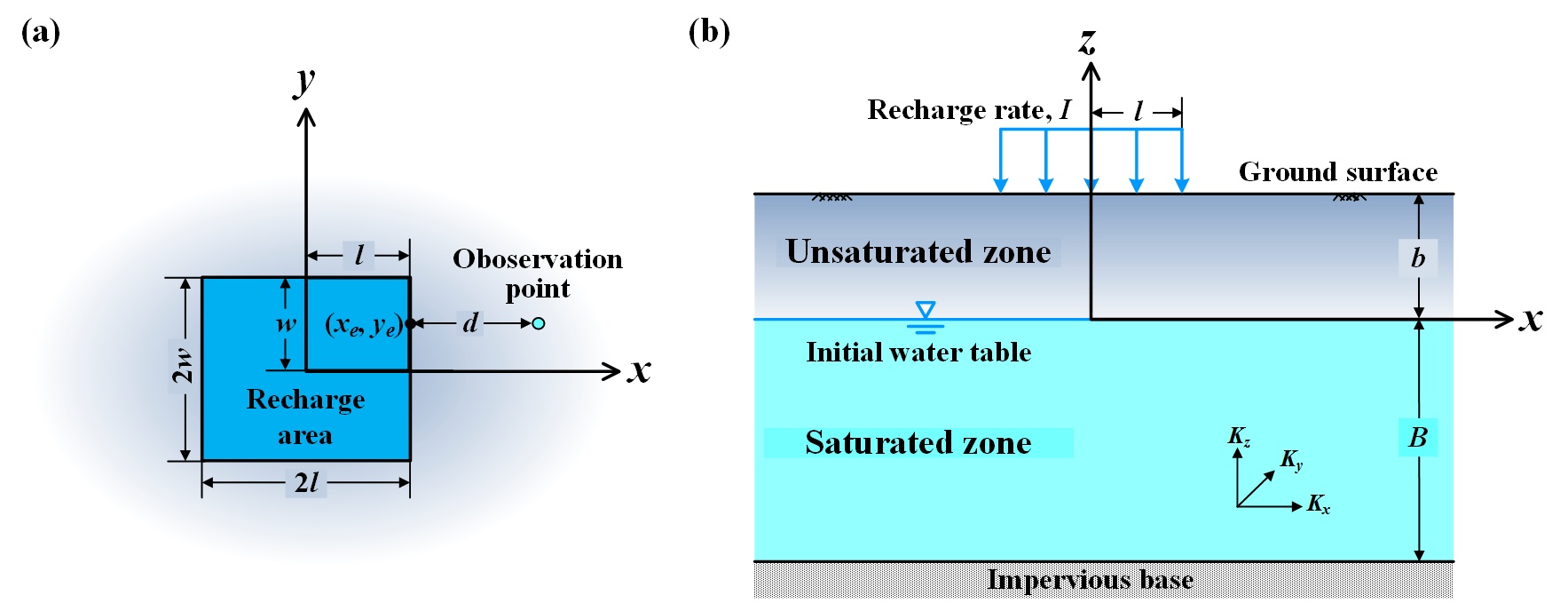
Figure 1Schematic diagram of unsaturated–saturated flow in an unconfined aquifer system with localized recharge: (a) top view and (b) cross-sectional view.
The mathematical model for the aquifer system comprises two simultaneous equations for unsaturated and saturated flows. The equation for saturated flow in homogeneous and anisotropic aquifers is expressed as
where h(x, y, z, t) is the hydraulic head in the saturated zone; t is elapsed time since recharge began; Kx, Ky, and Kz are, respectively, the saturated hydraulic conductivities in the x, y, and z directions; Ss is the specific storage. Richards' equation for unsaturated flow is expressed as (Richards, 1931)
where ϕ(x, y, z, t) is the hydraulic head in the unsaturated zone. The relative hydraulic conductivity kr(ϕ) and specific moisture capacity C(ϕ) are defined by the Gardner constitutive model (Gardner, 1958) as
and
where Sy is the specific yield and a is the unsaturated exponent related to the pore-size distribution of a medium ranging from 0.2 to 5 m−1 (Philip, 1969). Substituting Eqs. (3) and (4) into Eq. (2) leads to
It is essentially nonlinear and solved with difficulty by analytical methods. Kroszynski and Dagan (1975) employed the approach of perturbation expansion to simplify Richards' equation as a first-order linearized equation and developed an approximate solution for unsaturated–saturated flow induced by well pumping. The approach is extensively used in many studies on unsaturated–saturated flow (e.g., Mathias and Butler, 2006; Tartakovsky and Neuman, 2007; Mishra et al., 2012; Liang et al., 2017a). The linearized version of Richards' equation is written as
The initial conditions for those two zones are
Because of symmetry of the recharge area along the x and y axes, the first quadrant (i.e., x≥0 and y≥0) of the flow domain is considered. Thus, all the horizontal outer boundaries are specified as the no-flow condition expressed as
where . The top boundary condition for the recharge area is denoted as
where I is a constant recharge rate and H() is the Heaviside step function. Note that Eq. (10) can be written as inside the recharge area and and denoted as outside that area. The impermeable boundary condition at the aquifer bottom is written as
The two continuity requirements of the hydraulic head and flux at the water table are expressed, respectively, as
and
The continuity conditions are valid when the water table change is less than 50 % of the initial saturated aquifer thickness, which is certified by a Hele-Shaw experiment (Marino, 1967).
Define the dimensionless variables and parameters as follows:
where the overbar represents a dimensionless variable or parameter. According to Eq. (14), the unsaturated–saturated flow model is rewritten as
where .
2.2 Laplace domain solution
The unsaturated–saturated flow model composed of Eqs. (15)–(23) is solved by the methods of Laplace and Fourier cosine transforms. The Laplace transform is defined as
with the property that
where represents the dimensionless hydraulic head in the Laplace domain, p is the Laplace transform parameter, , and is from Eq. (17). Using Eqs. (24) and (25) converts into , into , into , into , and ξ into ξ∕p. The model then becomes
and
subject to the transformed boundary conditions of with , at , and at . Moreover, the transformed continuity conditions are and at .
Afterward, one may take the double Fourier cosine transform that provides
and
where represents the dimensionless hydraulic head in the Fourier domain; ω1 and ω2 are the Fourier cosine transform parameters. The transform converts into , into ,
into , into , and into . Equations (26) and (27) hence become ordinary differential equations in terms of denoted, respectively, as
and
Similarly, the transformed boundary conditions are expressed as
and
The transformed continuity conditions are written as
and
Solving Eqs. (30) and (31) subject to Eqs. (32)–(35) and then taking the inverse Fourier cosine transform leads to the solutions in the Laplace domain written as
and
with
Note that Eq. (36a) is the solution for unsaturated flow, while Eq. (36b) is that for saturated flow. The inverse Laplace transform to both solutions may not be tractable. The numerical inversion of Laplace transform proposed by Stehfest (1970) is therefore used to obtain time-domain results of the solutions. The double integrals in the solutions can be evaluated numerically by the Gaussian quadrature (e.g., Gerald and Wheatley, 2004) using the dblquad Matlab built-in function (Gilat and Subramaniam, 2007) or the NIntegrate Mathematica built-in function (Wolfram, 1996).
2.3 Solution for the transient recharge rate
The present solution can be applied to the problem of time-varying recharge rates based on Duhamel's integral (Bear, 1979, p. 158). The dimensionless transient head solution subject to the dimensionless time-varying recharge rate can be expressed as
where τ is a dummy variable, denotes or for the initial dimensionless recharge rate , and represents or with replaced by . If Eq. (37) is not an integrable function, we can evaluate numerically through the discretization method that (Singh, 2005)
where signifies the dimensionless head solution at ; is a dimensionless time step; G(M) is called the ramp kernel; ξi and ξi−1 are, respectively, dimensionless recharge rates at and .
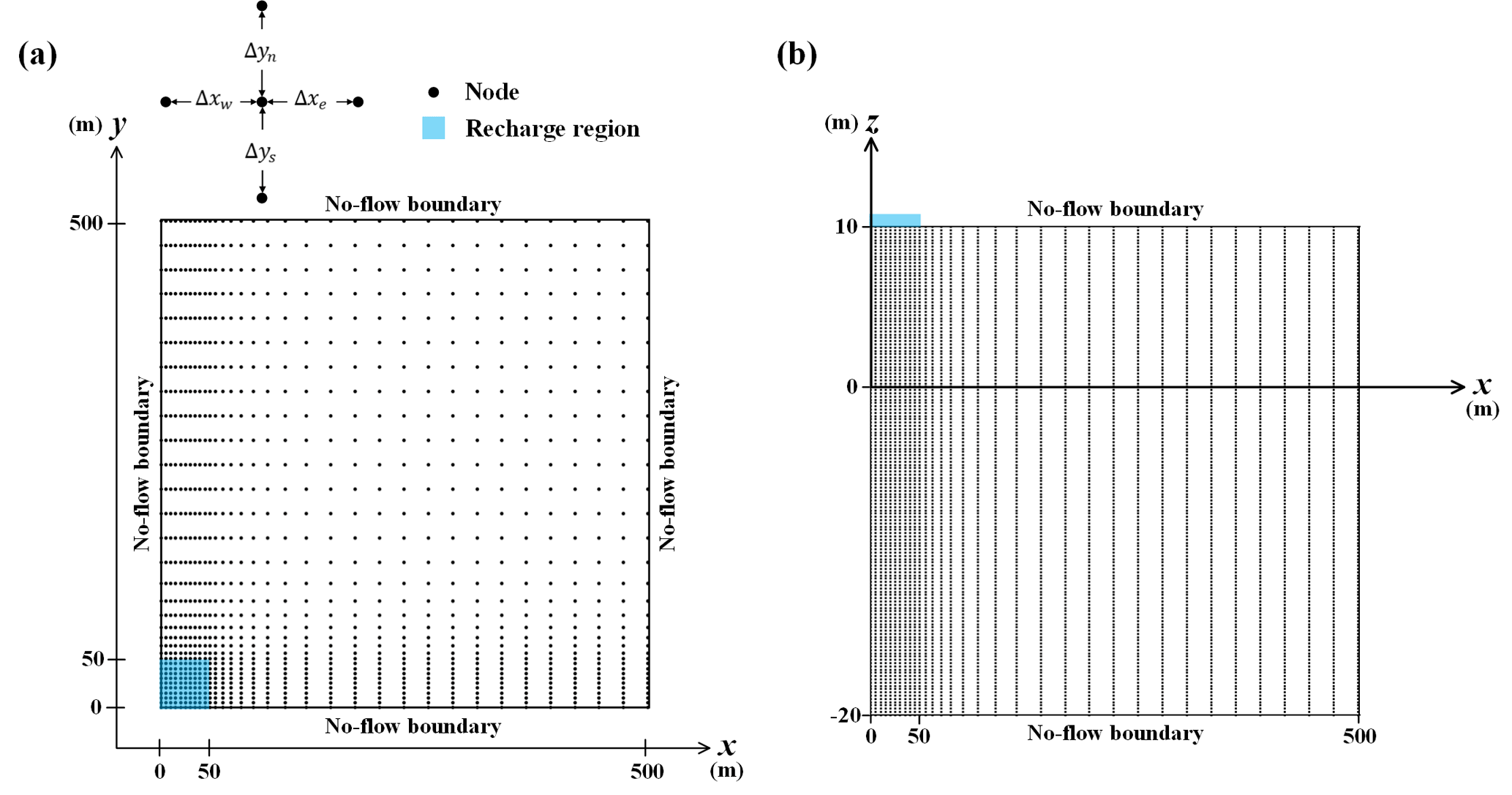
Figure 2Schematic diagram of finite-difference grids: (a) top view and (b) cross-sectional view.
2.4 Recharge efficiency
The percentage of the water from the localized recharge reaching the water table is defined as recharge efficiency (RE) (Munevar and Marino, 1999) written as
where the denominator is the volumetric rate of the water entering the aquifer system from the recharge, and the double integral is the sum of the infiltration flux at the water table. According to the dimensionless quantities defined in Eq. (14), Eq. (39) becomes
where represents RE in the Laplace domain and is defined in Eq. (36b). The RE increases from zero to a value equal to or below unity. The infiltration process does not affect the water table when RE =0. On the other hand, the water from the surface recharge totally arrives at the aquifer when RE =1.
2.5 Sensitivity analysis
The sensitivity analysis is commonly used to assess the change in the hydraulic head in response to a small change in a hydraulic parameter. The normalized sensitivity coefficient based on the present solution is defined as
where O represents the present solution for the unsaturated or saturated flow and Pi is the ith parameter. Equation (41) can be approximated as
where ΔPi is an increment set to 10−3Pi (Yeh et al., 2008). Note that a large value of indicates that the head is sensitive to the change in the target parameter.
2.6 Finite-difference solution
An iterative algorithm based on an implicit finite-difference approximation to Eq. (5) is developed to solve the nonlinear unsaturated–saturated flow model. Figure 2 shows the finite-difference grids in the simulation domains of m, m, and −20 m m discretized by a non-uniform grid with small grid sizes near the recharge area of m and m and large grid sizes away from that area. The domain falls in the first quadrant due to symmetrical flow to the x-axis and y-axis. The saturated thickness is 20 m and the unsaturated thickness is 10 m. All the boundaries except the recharge region are therefore under the no-flow condition. Equation (5) is approximated as
where is the hydraulic head in the unsaturated zone at a nodal point (i, j, k); superscript m represents one time step earlier than the present time denoted as superscript m+1; Δxw, Δxe, Δyn and Δys are grid sizes beside a nodal point (i, j, k) in the west, east, north and south, respectively; Δz is the grid size on the z-axis; Δt is the time step. Note that Eq. (43) reduces to the discretized expression of Eq. (6) when the quadratic terms are neglected. Similarly, Eq. (1) is approximated as
where is the hydraulic head in the saturated zone at a nodal point (i, j, k). The initial condition for each nodal point is expressed as
The no-flow condition specified at the outer boundaries shown in Fig. 2a and the bottom can be written as
where nx and ny are the total number of grids on the x- and y-axes, respectively. The top boundary condition is approximated as
where nz is the total number of grids on the z-axis. The grid sizes Δxw, Δxe, Δys, and Δyn are all 5 m inside the recharge area, while outside the area they gradually increase according to the formulas Δxe=1.2Δxw and Δyn=1.2Δys starting from m and m =6 m. Note that the largest grid size is set equal to 25 m for good accuracy in solution prediction. The grid size Δz is set to 0.1 m and the time step Δt is chosen as 0.1 days for the period of 0–2.5 days and 0.25 days for 2.5–100 days. The total number of nodal points is 327 789. The values of the hydraulic parameters are shown in Table 1.
The head solution to the nonlinear model of Eqs. (43)–(49) is obtained by an iteration method. Initially, the quadratic terms in Eq. (43) are assumed as with
where superscript (n) represents the nth iteration and gradients , , and cause a linearized Eq. (43) because they are known head values from the previous iteration. At the first time step (i.e., t=Δt, m=2), the first iteration solves a system of Eqs. (44)–(49) and the linearized Eq. (43) with and obtains the numerical solution of at each nodal point. The second iteration obtains with updated values of , , and from the previous result of . Repeat this iteration process for n≥3 until the convergence condition of at each nodal point in the unsaturated zone is satisfied. The last result of is therefore the head solution to the nonlinear model. Similarly, the iteration process is applied to obtain for m≥3 at the other time steps (i.e., t=2Δt, 3Δt,…) with the convergence condition . Note that the first iteration at each time step calculates , , and using obtained at the previous time step.
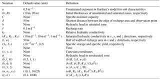
The default values of the parameters and variables used in the calculation of the present solution are listed in Table 1. In Sect. 3.1, the error arising from neglecting the process of infiltration in the unsaturated zone is examined. In Sect. 3.2, the recharge efficiency associated with the properties of the unsaturated zone is investigated. In Sect. 3.3, the sensitivity analysis of the hydraulic head in the unsaturated zone in regard to various hydraulic parameters is discussed. In Sect. 3.4, the present solution is compared with a finite-difference solution. In Sect. 3.5, the present solution is applied to a field problem of artificial recharge.
3.1 Effect of unsaturated flow on head distributions in aquifers

Figure 3Temporal distributions of the dimensionless head in the saturated zone predicted by the present solution and Chang et al.'s (2016) solution for different pairs of (α, ) representing the effect of unsaturated flow.
Here we investigate the difference between the present solution and Chang et al.'s (2016) analytical solution to explore the effect of unsaturated flow on the head distributions in the aquifer. Chang et al.'s (2016) solution considers 3-D saturated flow in an unconfined aquifer with localized recharge but neglects the effect of unsaturated flow. One might expect that the difference will mainly be dominated by the magnitudes of parameters α (dimensionless unsaturated exponent) and (dimensionless unsaturated thickness). Figure 3 displays the predicted temporal head distributions at ( by their solution and the present solution, Eq. (36b), for different pairs of (α, ) with α=102 or 103 and from 10−3 to one. Significant difference in predicted by both solutions can be seen except for the cases (α, , (103, 10−1), and (103, 10−2) shown in the figure. The result indicates that the thickness of the unsaturated zone is less than 10 % of the saturated aquifer thickness (i.e., ) for obtaining close predictions from both solutions. When , both solutions disagree if α=102 and agree well if α=103, indicating that the magnitude of the product (=ab) should at least be 10 (i.e., ) for good agreement of both solutions. It is worth noting that both solutions disagree even for a much thinner unsaturated zone as compared with the aquifer (i.e., ) because of . Additionally, the curves for α=10 all disagree with Chang et al.'s (2016) solution, whereas the curves for α=104 match with this solution except for two cases where (α, and (104, 1) (not shown in the figure). Judging from the above, one can recognize that the effect of unsaturated flow on the predicted head in saturated aquifers is negligible when and . A great number of existing analytical solutions ignoring unsaturated flow give accurate predictions only when those two inequalities are satisfied (e.g., Chang and Yeh, 2007; Illas et al., 2008; Bansal and Teloglou, 2013). Otherwise, significant deviations will happen in their predictions.
3.2 Effect of unsaturated flow on recharge efficiency
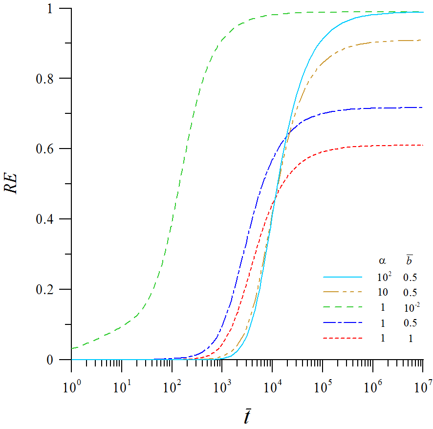
Figure 4Temporal distribution curves of the recharge efficiency (RE) for different pairs of (α, ) representing the effect of unsaturated flow.
The effect of the unsaturated zone on the RE is explored based on the curves of the RE versus shown in Fig. 4 plotted using Eq. (40) for different pairs of , (10, 0.5), (1, 0.01), (1, 0.5), and (1, 1). For a given , the RE increases with α for a fixed and decreasing for a fixed α. After , the RE approaches an ultimate value equalling unity when and (1, 0.01), 0.9 when , 0.7 when , and 0.6 when . Those results imply that the ultimate recharge efficiency (URE) depends on the magnitudes of both α and . Figure 5 illustrates contours of the URE at in the ranges of and . The URE approaches unity when or α>20. In contrast, it is below 0.9 and related to a given pair (α, ) when and α<10. It is clearly seen that the RE is great for a large α and/or a small . Those results provide useful information in the estimation of the amount of water from the recharge entering the aquifer. Notice that the case of URE <1 may be due to the problem that unsaturated flow is influenced by the water retention capacity and diffusivity in the horizontal direction.
3.3 Sensitivity analysis for flow in unsaturated zone
Chang et al. (2016) performed the sensitivity analysis to investigate the sensitivity of the hydraulic head in saturated aquifers to the change in each of the aquifer parameters. This section focuses on the sensitivity analysis of the head in the unsaturated zone. Consider the recharge area of m and m and the observation points A at (0, 0, 5 m) under the area and B at (100 m, 0, 5 m) beside the area. Other values of the parameters are given in Table 1. The temporal distribution curves of the normalized sensitivity coefficient Si,t predicted by Eq. (42) to each of the parameters a, l, w, Ss, Sy, Kx, Ky, and Kz are exhibited in Fig. 6a for point A and Fig. 6b for point B. At a given time, a positive Si,t means that the change in the specific parameter causes the increase in the head. In contrast, a negative Si,t signifies that the change leads to the head decrease. The magnitude of the head remains unchanged when . Obviously, the parameters l, w, Sy, Kx, and Ky are important factors affecting the predicted head observed at points A and B, revealing that those parameters should be included in the flow model. The head at point A is sensitive to the changes in a and Kz, but that at point B is insensitive. The result implies that unsaturated flow prevails under the recharge area but does not away from the area. In addition, the coefficient Si,t to Ss almost equals zero over the entire recharge period, indicating that the change in Ss does not affect the predicted head in the unsaturated zone.
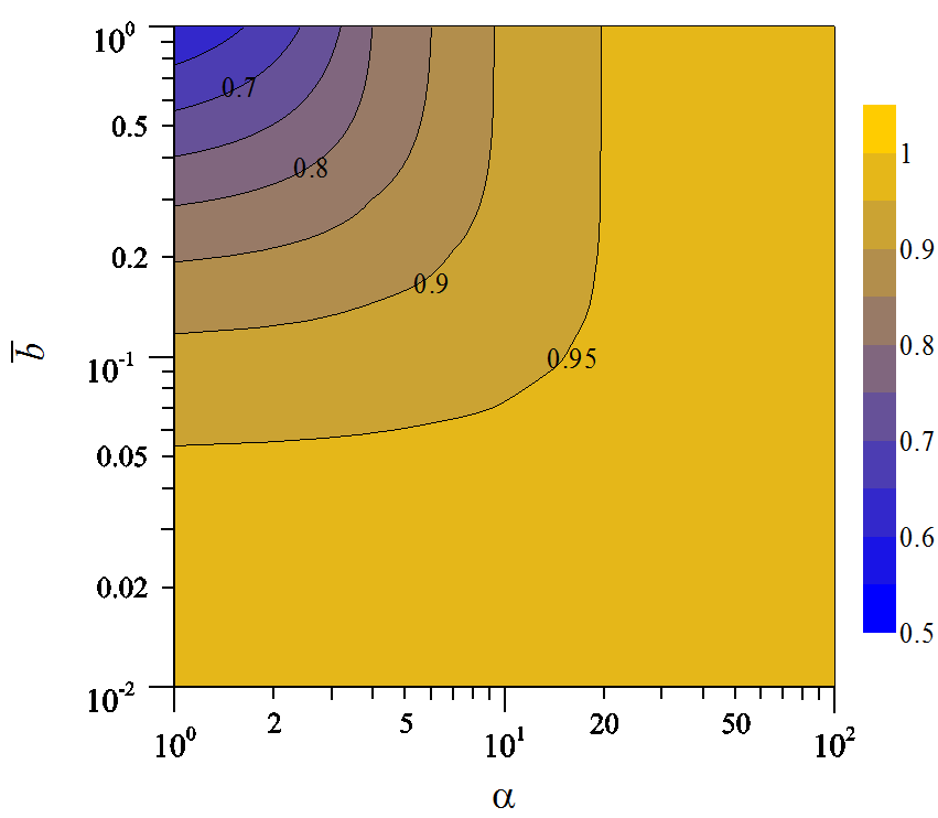
Figure 5Contours of the ultimate recharge efficiency (URE) plotted at for various values of α and .
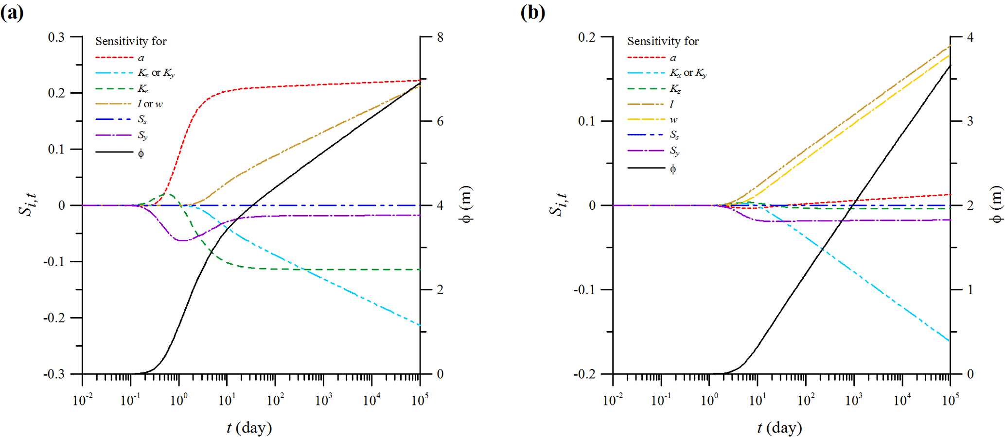
Figure 6Temporal distribution curves of the normalized sensitivity coefficients for the hydraulic head in the unsaturated zone in response to the change in each of the parameters a, l, w, Ss, Sy, Kx, Ky, and Kz observed at (a) (0, 0, 5 m) under the recharge area and (b) (100 m, 0, 5 m) beside the area.
3.4 Validation of the present solution
The finite-difference solution to the unsaturated–saturated flow model based on the nonlinear and linearized versions of Richards' equation, Eqs. (5) and (6), has been developed and described in Sect. 2.6. It is used to validate the present solution. Figure 7 demonstrates temporal head distributions observed at (25 m, 0, 5 m) and (25 m, 0, −10 m) under the recharge area and at (94.65 m, 0, 5 m) and (94.65 m, 0, −10 m) beside the area. The figure displays good agreement on the predicted head distributions from both the solutions. It is noteworthy that numerous attempts had been made by scholars to examine the accuracy of the linearized version of Richards' equation (e.g., Kroszynski and Dagan, 1975; Mishra and Neuman, 2010; Liang et al., 2017b). They also revealed that the linearized equation causes insignificant deviation in model predictions. We therefore conclude that the present solution is correctly developed and fairly predicts the hydraulic head for the unsaturated–saturated flow induced by localized recharge.
3.5 Application of the present solution to the field experiment
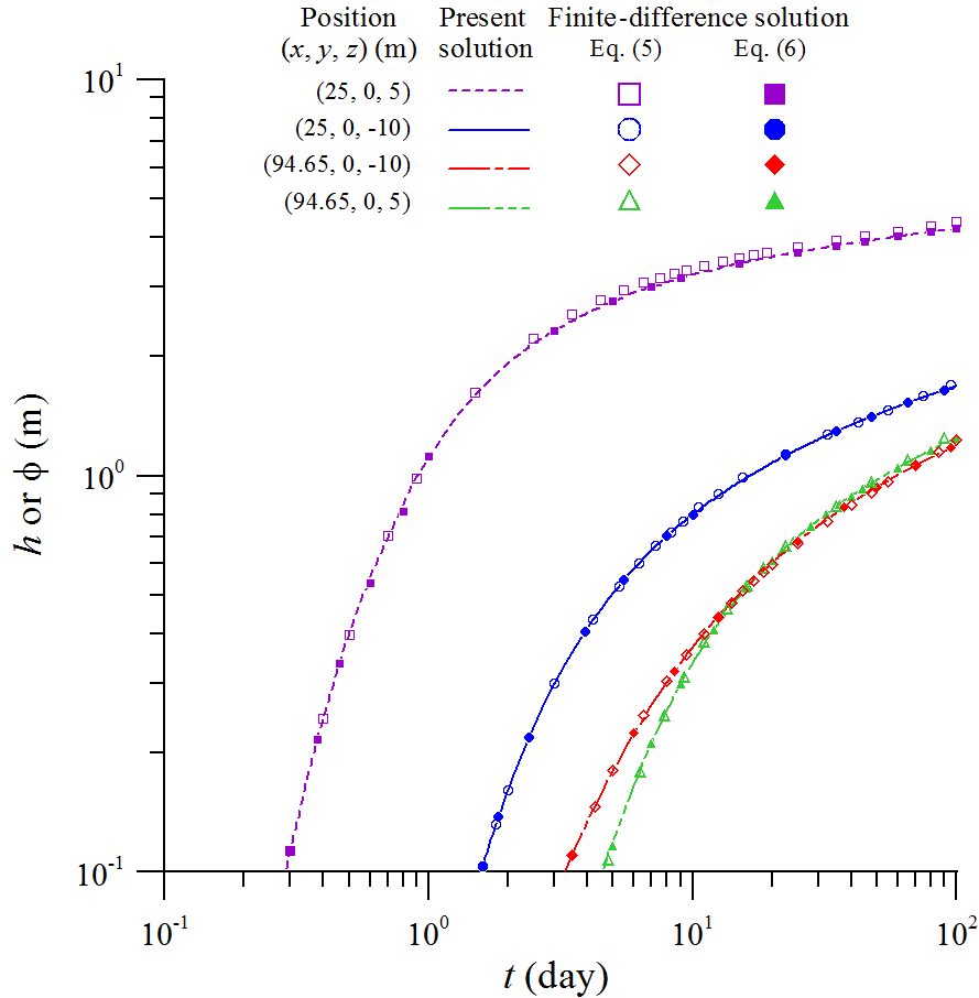
Figure 7Temporal distributions of the hydraulic head predicted by the present solution and the finite-difference solution based on Richards' equation, Eq. (5), and its linearized version, Eq. (6), observed at (25 m, 0, 5 m) and (25 m, 0, −10 m) under the recharge area and at (94.65 m, 0, 5 m) and (94.65 m, 0, −10 m) beside the area.
Bianchi and Haskell (1968) executed a field experiment of artificial recharge from two ponds on an alluvial fan in Fresno County, California. Pond No. 2 was within a square of 90 m × 90 m on the ground. The average recharge rate of the pond was 0.107 m d−1. The initial water table was 6.4 m below the ground and 24.384 m over the impervious aquifer bottom. The entire recharge period was 10.92 days on record. The values of the aquifer parameters obtained from well test data were Kx=7.925 m d−1 and Sy=0.022. There are 19 observation data of the water table rise beneath the center of the pond versus time shown in Fig. 8. We apply the least square method using the Mathematica FindRoot built-in function (Wolfram, 1996) to estimate five parameters a, Kx=Ky, Kz, Ss, and Sy based on the data and the present solution. The estimated values are a=0.388 m−1, Kx=5.642 m d−1, Kz=1.573 m d−1, m−1, and Sy=0.102, which are all in the reasonable ranges of their parameter values; they are m−1 (Philip, 1969), m d−1, , , and .3 for sandy aquifers (Freeze and Cherry, 1979, p. 604). Figure 8 demonstrates 19 observed data of the water table rise, the predictions from Glover's (1960) solution with Kx=7.925 m d−1 and Sy=0.022 provided in Bianchi and Haskell (1968), and the present solution with the five estimated parameters. The Glover solution was developed by assuming that the flow is radially outward from a circular recharge pond with an equivalent area to the square of 90 m × 90 m and the unsaturated flow above water table is neglected. The predictions from the present solution agree well with the observed data, but those from Glover's solution do not, indicating that the effect of unsaturated flow had better be considered because and in this case do not satisfy the condition of and concluded in Sect. 3.1. From those discussed above, the present solution has been shown to be applicable to a real-world problem for unsaturated–saturated flow due to a recharge pond.
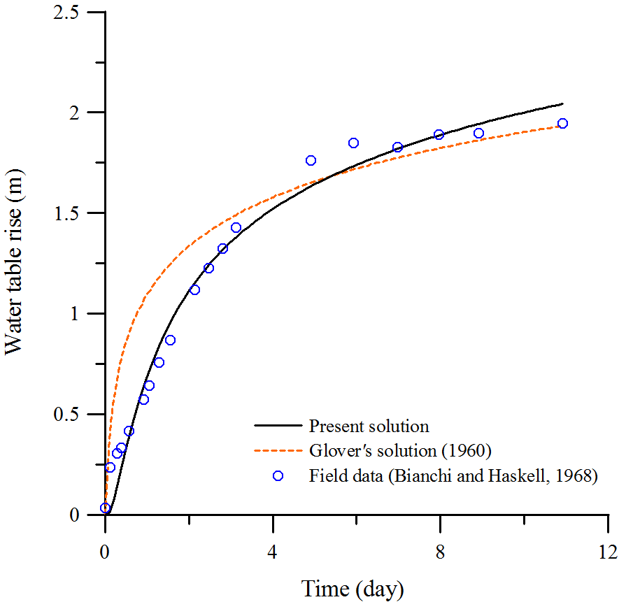
Figure 8Comparison of the water table rise predicted by the present solution and Glover's (1960) solution with field-observed data given in Bianchi and Haskell (1968).
This study develops a novel mathematical model depicting 3-D unsaturated–saturated flow for the process that surface water recharge passes through an unsaturated zone and flows down to an unconfined aquifer. The Richards equation is considered to delineate unsaturated flow induced by infiltration due to recharge from the ground surface. The Gardner model is used to describe the unsaturated soil characteristics. The transient groundwater flow equation is then employed to describe the rise of the hydraulic head in the aquifer in response to the water flow from the unsaturated zone. Both equations are coupled by the continuity equations of the head and flux at the water table. The head solution to the model is derived by means of the Laplace transform and Fourier cosine transform. The recharge efficiency defined as the percentage of the water from the recharge down to the aquifer is clearly discussed. The sensitivity analysis is performed to investigate the head response to the change in each of the hydraulic parameters in the unsaturated zone. The present solution agrees well with the finite-difference solution in predicting the time-varying head for the unsaturated–saturated flow model. In addition, the present solution is applied to study the observed data from a field experiment conducted by Bianchi and Haskell (1968). On the basis of the studies obtained from the present solution, the following conclusions can be drawn.
The effect of unsaturated flow on the hydraulic head in the aquifer is ignorable when the product of the unsaturated exponent (a) and initial unsaturated thickness (b) is greater than 10 (i.e., ab≥10) and the unsaturated thickness is less than 10 % of the initial aquifer thickness (B) (i.e., ). Otherwise, the effect should be considered to avoid large deviations in calculating the head in the aquifer. Existing models considering only saturated flow can predict accurate results only when these two inequalities are satisfied.
The recharge efficiency initially equals zero, increases with time, and finally approaches a constant value (below or equal to unity) depending on the values of α(=aB) and .
The ultimate recharge efficiency approaches unity when or α>20 but less than 90 % when and α<10. In other words, the surface source supplies more recharge water to the aquifer if the unsaturated zone has a large α and/or a small .
The results of the sensitivity analysis indicate that the parameter a, l, or w causes positive influence but Sy, Kx, Ky, or Kz produces negative impact on the predicted head in the unsaturated zone. The head under the recharge area is sensitive to the changes in a and Kz, but that beside the area is not. Moreover, the head is rather insensitive to the change in Ss.
The field-observed data and Glover's (1960) solution are provided in Bianchi and Haskell (1968). The data sets of Chang et al.'s (2016) solution, the present solution, and the finite-difference solution are available upon request.
C-HC conceived the presented idea, developed the semi-analytical solution and code for the model, and performed the results in the figures. C-SH developed the code for the finite-difference simulations. H-DY supervised the findings of this work. All authors discussed the results and contributed to the final manuscript.
The authors declare that they have no conflict of interest.
This research has been supported in part by the grants from the Fundamental
Research Funds for the Central Universities (2018B00114) and the Taiwan
Ministry of Science and Technology under the contract numbers MOST
105-2221-E-009-043-MY2 and MOST 106-2221-E-009-066. The authors are indebted
to the thoughtful and helpful comments of the editor and two
reviewers.
Edited by: Philippe Ackerer
Reviewed by: two anonymous referees
Bansal, R. K. and Teloglou, I. S.: An analytical study of groundwater fluctuations in unconfined leaky aquifers induced by multiple localized recharge and withdrawal, Global Nest J., 15, 394–407, 2013.
Batu, V.: Flow net for unsaturated infiltration from periodic strip sources, Water Resour. Res., 16, 284–288, 1980.
Bear, J.: Hydraulics of Groundwater, McGraw-Hill, New York, 1979.
Bianchi, W. C. and Haskell, E. E.: Field observations compared with Dupuit-Forchheimer theory for mound heights under a recharge basin, Water Resour. Res., 4, 1049–1057, https://doi.org/10.1029/WR004i005p01049, 1968.
Chang, C.-H., Huang, C.-S., and Yeh, H.-D.: Technical Note: Three-dimensional transient groundwater flow due to localized recharge with an arbitrary transient rate in unconfined aquifers, Hydrol. Earth Syst. Sci., 20, 1225–1239, https://doi.org/10.5194/hess-20-1225-2016, 2016.
Chang, Y. C. and Yeh, H. D.: Analytical solution for groundwater flow in an anisotropic sloping aquifer with arbitrarily located multiwells, J. Hydrol., 347, 143–152, 2007.
Chen, J. M., Tan, Y. C., Chen, C. H., and Parlange, J. Y.: Analytical solutions for linearized Richards' equation with arbitrary time-dependent surface fluxes, Water Resour. Res., 37, 1091–1093, 2001a.
Chen, J. M., Tan, Y. C., and Chen, C. H.: Multidimensional infiltration with arbitrary surface fluxes, J. Irrig. Drain. E-Asce, 127, 370–377, https://doi.org/10.1061/(asce)0733-9437(2001)127:6(370), 2001b.
Freeze, R. A. and Cherry, J. A.: Groundwater, Prentice-Hall, Englewood Cliffs, New Jersey, 1979.
Gardner, W. R.: Some steady-state solutions of the unsaturated moisture flow equation with application to evaporation from a water table, Soil Sci., 85, 228–232, 1958.
Gerald, C. F. and Wheatley, P. O.: Applied Numerical Analysis, 7th Edn., Pearson-Wesley, Boston, 2004.
Gilat, A. and Subramaniam, V.: Numerical Methods for Engineers and Scientists: An Introduction with Applications Using MATLAB, John Wiley & Sons, Hoboken, New Jersey, 2007.
Glover, R. E.: Mathematical derivations as pertain to groundwater recharge, Agricultural Research Service, US Department of Agriculture, Colorado, 1960.
Huang, R. Q. and Wu, L. Z.: Analytical solutions to 1-D horizontal and vertical water infiltration in saturated/unsaturated soils considering time-varying rainfall, Comput. Geotech., 39, 66–72, https://doi.org/10.1016/j.compgeo.2011.08.008, 2012.
Illas, T. S., Thomas, Z. S., and Andreas, P. C.: Water table fluctuation in aquifers overlying a semi-impervious layer due to transient recharge from a circular basin, J. Hydrol., 348, 215–223, 2008.
Kroszynski, U. I. and Dagan, G.: Well pumping in unconfined aquifers: The influence of the unsaturated zone, Water Resour. Res., 11, 479–490, https://doi.org/10.1029/WR011i003p00479, 1975.
Liang, X. Y., Zhan, H. B., Zhang, Y.-K., and Liu, J.: On the coupled unsaturated–saturated flow process induced by vertical, horizontal, and slant wells in unconfined aquifers, Hydrol. Earth Syst. Sci., 21, 1251–1262, https://doi.org/10.5194/hess-21-1251-2017, 2017a.
Liang, X. Y., Zhan, H. B., Zhang, Y. K., and Schilling, K.: Base flow recession from unsaturated-saturated porous media considering lateral unsaturated discharge and aquifer compressibility, Water Resour. Res., 53, 7832–7852, https://doi.org/10.1002/2017WR020938, 2017b.
Marino, M. A.: Hele-Shaw model study of the growth and decay of groundwater ridges, J. Geophys. Res., 72, 1195–1205, https://doi.org/10.1029/JZ072i004p01195, 1967.
Mathias, S. A. and Butler, A. P.: Linearized Richards' equation approach to pumping test analysis in compressible aquifers, Water Resour. Res., 42, W06408. https://doi.org/10.1029/2005WR004680, 2006.
Mishra, P. K. and Neuman, S. P.: Improved forward and inverse analyses of saturated-unsaturated flow toward a well in a compressible unconfined aquifer, Water Resour. Res., 46, W07508, https://doi.org/10.1029/2009wr008899, 2010.
Mishra, P. K. and Neuman, S. P.: Saturated-unsaturated flow to a well with storage in a compressible unconfined aquifer, Water Resour. Res., 47, W05553, https://doi.org/10.1029/2010wr010177, 2011.
Mishra, P. K., Vesselinov, V. V., and Kuhlman, K. L.: Saturated-unsaturated flow in a compressible leaky-unconfined aquifer, Adv. Water Resour., 42, 62–70, 2012.
Munevar, A. and Marino, M. A.: Modeling analysis of ground water recharge potential on alluvial fans using limited data, Ground Water, 37, 649–659, 1999.
Philip, J. R.: Theory of infiltration, Adv. Hydrosci., 5, 215–305, 1969.
Protopapas, A. L. and Bras, R. L.: Analytical solutions for unsteady multidimensional infiltration in heterogeneous soils, Water Resour. Res., 27, 1029–1034, 1991.
Richards, L. A.: Capillary conduction of liquids through porous mediums, J. Appl. Phys., 1, 318-333, https://doi.org/10.1063/1.1745010, 1931.
Scudeler, C., Pangle, L., Pasetto, D., Niu, G.-Y., Volkmann, T., Paniconi, C., Putti, M., and Troch, P.: Multiresponse modeling of variably saturated flow and isotope tracer transport for a hillslope experiment at the Landscape Evolution Observatory, Hydrol. Earth Syst. Sci., 20, 4061–4078, https://doi.org/10.5194/hess-20-4061-2016, 2016.
Shi, P. F., Yang, T., Zhang, K., Tang, Q. H., Yu, Z. B., and Zhou, X. D.: Large-scale climate patterns and precipitation in an arid endorheic region: linkage and underlying mechanism, Environ. Res. Lett., 11, 044006, https://doi.org/10.1088/1748-9326/11/4/044006, 2016.
Siltecho, S., Hammecker, C., Sriboonlue, V., Clermont-Dauphin, C., Trelo-ges, V., Antonino, A. C. D., and Angulo-Jaramillo, R.: Use of field and laboratory methods for estimating unsaturated hydraulic properties under different land uses, Hydrol. Earth Syst. Sci., 19, 1193–1207, https://doi.org/10.5194/hess-19-1193-2015, 2015.
Singh, S. K.: Rate and volume of stream flow depletion due to unsteady pumping, J. Irrig. Drain. E.-Asce, 131, 539–545, 2005.
Srivastava, R. and Yeh, T. C. J.: Analytical solutions for one-dimensional, transient infiltration toward the water-table in homogeneous and layered soils, Water Resour. Res., 27, 753–762, 1991.
Stehfest, H.: Numerical inversion of Laplace transforms, Commun. ACM, 13, 47–49, https://doi.org/10.1145/361953.361969, 1970.
Tartakovsky, G. D. and Neuman, S. P.: Three-dimensional saturated-unsaturated flow with axial symmetry to a partially penetrating well in a compressible unconfined aquifer, Water Resour. Res., 43, W01410, https://doi.org/10.1029/2006WR005153, 2007.
Tracy, F. T.: Three-dimensional analytical solutions of Richards' equation for a box-shaped soil sample with piecewise-constant head boundary conditions on the top, J. Hydrol., 336, 391–400, 2007.
Wang, H. and Li, J.: Analytical solutions to the one-dimensional coupled seepage and deformation of unsaturated soils with arbitrary nonhomogeneous boundary conditions, Transport Porous. Med., 108, 481–496, 10.1007/s11242-015-0485-x, 2015.
Wang, X.-S., Ma, M.-G., Li, X., Zhao, J., Dong, P., and Zhou, J.: Groundwater response to leakage of surface water through a thick vadose zone in the middle reaches area of Heihe River Basin, in China, Hydrol. Earth Syst. Sci., 14, 639–650, https://doi.org/10.5194/hess-14-639-2010, 2010.
Warrick, A. W.: Analytical solutions to the one-dimensional linearized moisture flow equation for arbitrary input, Soil Sci., 120, 79–84, 1975.
Wolfram, S.: The Mathematica Book, 3rd Edn., Cambridge University Press, Cambridge, England, 1996.
Wu, L. Z., Zhang, L. M., and Huang, R. Q.: Analytical solution to 1D coupled water infiltration and deformation in two-layer unsaturated soils, Int. J. Numer. Anal. Met., 36, 798–816, 2012.
Wu, L. Z., Selvadurai, A. P. S., and Huang, R. Q.: Two-dimensional coupled hydromechanical modeling of water infiltration into a transversely isotropic unsaturated soil region, Vadose Zone J., 12, vzj2013.04.0072, https://doi.org/10.2136/vzj2013.04.0072, 2013.
Yang, T., Wang, C., Chen, Y. N., Chen, X., and Yu, Z. B.: Climate change and water storage variability over an arid endorheic region, J. Hydrol., 529, 330–339, 2015.
Yeh, H. D., Chang, Y. C., and Zlotnik, V. A.: Stream depletion rate and volume from groundwater pumping in wedge-shape aquifers, J. Hydrol., 349, 501–511, 2008.
The requested paper has a corresponding corrigendum published. Please read the corrigendum first before downloading the article.
- Article
(1085 KB) - Full-text XML