the Creative Commons Attribution 4.0 License.
the Creative Commons Attribution 4.0 License.
 | 07 Aug 2018
Technical note: Bathymetry observations of inland water bodies using a tethered single-beam sonar controlled by an unmanned aerial vehicle
Daniel Olesen
Jakob Jakobsen
Cecile Marie Margaretha Kittel
Sheng Wang
Monica Garcia
Peter Bauer-Gottwein
High-quality bathymetric maps of inland water bodies are a common requirement for hydraulic engineering and hydrological science applications. Remote sensing methods, such as space-borne and airborne multispectral imaging or lidar, have been developed to estimate water depth, but are ineffective for most inland water bodies, because of the attenuation of electromagnetic radiation in water, especially under turbid conditions. Surveys conducted with boats equipped with sonars can retrieve accurate water depths, but are expensive, time-consuming, and unsuitable for unnavigable water bodies.
We develop and assess a novel approach to retrieve accurate and high-resolution bathymetry maps. We measured accurate water depths using a tethered floating sonar controlled by an unmanned aerial vehicle (UAV) in a lake and in two different rivers located in Denmark. The developed technique combines the advantages of remote sensing with the potential of bathymetric sonars. UAV surveys can be conducted also in unnavigable, inaccessible, or remote water bodies. The tethered sonar can measure bathymetry with an accuracy of ∼2.1 % of the actual depth for observations up to 35 m, without being significantly affected by water turbidity, bed form, or bed material.
- Article
(7848 KB) -
Supplement
(107 KB) - BibTeX
- EndNote


Accurate topographic data from the riverbed and floodplain areas are crucial elements in hydrodynamic models. Detailed bathymetry maps of inland water bodies are essential for simulating flow dynamics and forecasting flood hazard (Conner and Tonina, 2014; Gichamo et al., 2012; Schäppi et al., 2010), predicting sediment transport and streambed morphological evolution (Manley and Singer, 2008; Nitsche et al., 2007; Rovira et al., 2005; Snellen et al., 2011), and monitoring instream habitats (Brown and Blondel, 2009; Powers et al., 2015; Strayer et al., 2006; Walker and Alford, 2016). Whereas exposed floodplain areas can be directly monitored from aerial surveys, riverbed topography is not directly observable from airborne or space-borne methods (Alsdorf et al., 2007). Thus, there is a widespread global deficiency in bathymetry measurements of rivers and lakes.
Within the electromagnetic spectrum, visible wavelengths have the greatest atmospheric transmittance and the smallest attenuation in water. Therefore, remote sensing imagery from satellites, such as Landsat (Liceaga-Correa and Euan-Avila, 2002), QuickBird (Lyons et al., 2011), IKONOS (Stumpf et al., 2003), WorldView-2 (Hamylton et al., 2015; Lee et al., 2011), and aircrafts (Carbonneau et al., 2006; Marcus et al., 2003), has been used to monitor the bathymetry of inland water bodies. However, bathymetry can only be derived from optical imagery when water is very clear and shallow, the sediment is comparatively homogeneous, and atmospheric conditions are favorable (Legleiter et al., 2009; Lyzenga, 1981; Lyzenga et al., 2006; Overstreet and Legleiter, 2017). Thus, passive remote sensing applications are limited to shallow gravel-bed rivers, in which water depth is on the order of the Secchi depth (depth at which a Secchi disk is no longer visible from the surface).
Similarly, airborne lidars operating with a green wavelength can be applied to retrieve bathymetry maps (Bailly et al., 2010; Hilldale and Raff, 2008; Legleiter, 2012), but also this method is limited by water turbidity, which severely restricts the maximum depth to generally 2–3 times the Secchi depth (Guenther, 2001; Guenther et al., 2000).
Because of satellite or aircraft remote sensing limitations, field surveys, which are expensive and labor intensive, are normally required to obtain accurate bathymetric cross sections of river channels. Some preliminary tests using a green wavelength (λ= 532 nm) terrestrial laser scanning (TLS) for surveying submerged areas were performed (Smith et al., 2012; Smith and Vericat, 2014). However, TLS suffers from similar limitations as lidar. Furthermore, the highly oblique scan angles of TLS make refraction effects more problematic (Woodget et al., 2015) and decrease returns from the bottom while increasing returns from the water surface (Bangen et al., 2014). Therefore, field surveys are normally performed using single-beam or multi-beam swath sonars transported on manned boats or more recently on unmanned vessels (e.g., Brown et al., 2010; Ferreira et al., 2009; Giordano et al., 2015) . However, boats cannot be employed along unnavigable rivers and require sufficient water depth for navigation.
Unmanned aerial vehicles (UAVs) offer the advantage of enabling a rapid characterization of water bodies in areas that may be difficult to access by human operators (Tauro et al., 2015b). Bathymetry studies using UAVs are so far restricted to (i) spectral signature-depth correlation based on passive optical imagery (Flener et al., 2013; Lejot et al., 2007) or (ii) DEM (digital elevation model) generation through stereoscopic techniques from through-water pictures, correcting for the refractive index of water (Bagheri et al., 2015; Dietrich, 2016; Tamminga et al., 2014; Woodget et al., 2015).
The high cost, size, and weight of bathymetric lidars severely limit their implementation on UAVs. An exception is the novel topo-bathymetric laser profiler, bathymetric depth finder BDF-1 (Mandlburger et al., 2016). This lidar profiler can retrieve measurements of up to 1–1.5 times the Secchi depth; thus, it is only suitable for shallow gravel-bed water bodies. The system weighs ∼5.3 kg and requires a large UAV platform (e.g., multi-copters with a weight of ∼25 kg).
To overcome these limitations, we assess a new operational method to estimate river bathymetry in deep and turbid rivers. This new technique involves deploying an off-the-shelf, floating sonar, tethered to and controlled by a UAV. With this technique we can combine (i) the advantages of UAVs in terms of the ability to survey remote, dangerous, unnavigable areas with (ii) the capability of bathymetric sonars to measure bathymetry in deep and turbid inland water bodies.
UAV measurements of water depth (i.e., elevation of the water surface above the bed) can enrich the set of available hydrological observations along with measurements of water surface elevation (WSE), i.e., elevation of the water surface above sea level (Bandini et al., 2017; Ridolfi and Manciola, 2018; Woodget et al., 2015), and surface water flow (Detert and Weitbrecht, 2015; Tauro et al., 2015a, 2016; Virili et al., 2015).
The UAV used for this study was the off-the-shelf DJI hexa-copter Spreading Wings S900 equipped with a DJI A-2 flight controller.
2.1 UAV payload
The UAV was equipped with a Global Navigation Satellite System (GNSS) receiver for retrieving accurate position, an inertial measurement unit (IMU) to retrieve angular and linear motion, and a radar system to measure the range to water surface. A picture of the UAV and the tethered sonar is shown in Fig. 1.
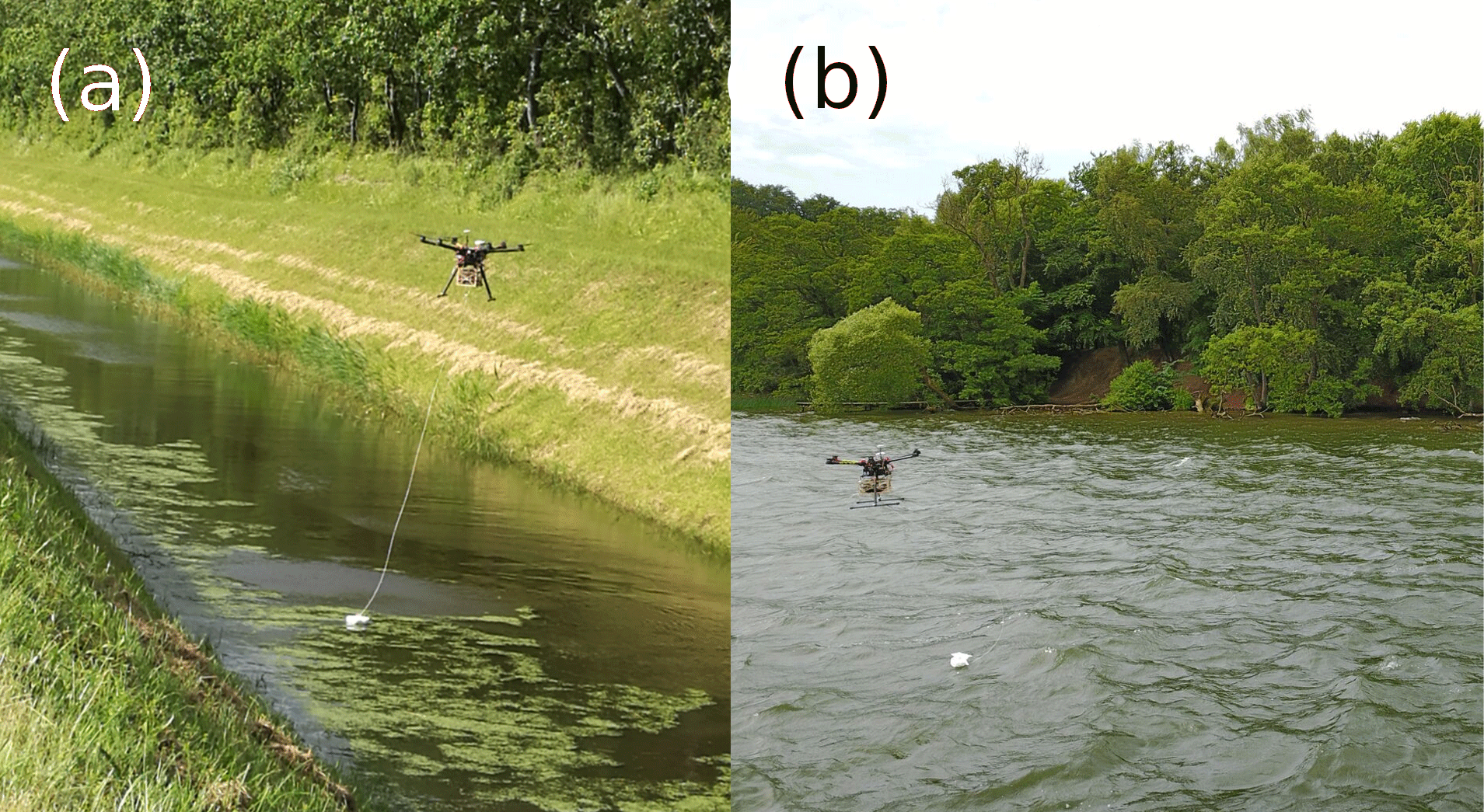
Figure 1Pictures of the UAV and the tethered sonar. These pictures were retrieved in (a) Marrebæk Kanal, Denmark; and (b) Furesø lake, Sjælland, Denmark. In (b) the drone was flown a few hundred meters from the shore and the picture was retrieved using an optical camera onboard an auxiliary UAV (DJI Mavic Pro).
The onboard GNSS system is a NovAtel receiver (OEM628 board) with an Antcom (3G0XX16A4-XT-1-4-Cert) dual frequency GPS and GLONASS flight antenna. The UAV horizontal and vertical position is estimated with ∼2–3 cm accuracy in carrier-phase differential GPS mode. The onboard inertial measurement unit is an Xsense MTi-10 series. The optical camera is a SONY RX-100 camera. The radar is an ARS 30X radar developed by Continental. The radar and GNSS systems are the same instrumentation as described in Bandini et al. (2017), in which WSE was measured by subtracting the range measured by the radar (range between the UAV and the water surface) from the altitude observed by the GNSS instrumentation (i.e., altitude above reference ellipsoid, convertible into altitude above geoid level). In this research, the radar and GNSS instrumentation are used to (i) retrieve WSE and (ii) observe the accurate position of the tethered sonar.
2.2 Sonar instrumentation
The sonar used for this study was the Deeper Smart Sensor PRO+ manufactured by the company Deeper, UAB (Vilnius, Lithuania). It costs ∼ USD 240 and weighs ∼100 g.
The sonar is tethered to the UAV with a physical wire connection as shown in Fig. 2. For specific applications, the sonar can be lowered or raised using a remotely controlled lightweight wire winch, as shown in Fig. 2. The maximum extension of the wire was ∼5 m. A remotely controlled emergency hook can be installed to release the sonar in case of emergency (e.g., if the wire is caught in obstacles).
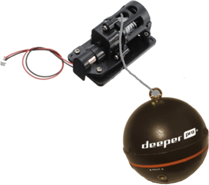
This sonar is a single-beam echo sounder with two frequencies: 290 and 90 kHz, with 15 and 55∘ beam angles, respectively. The 90 kHz frequency is developed to locate fish with a large scanning angle, while the narrow field of view of the 290 kHz frequency gives the highest bathymetric accuracy. For this reason, the 290 kHz frequency is used for observing the bottom structure. The sonar is capable of measuring depths up to 80 m and has a minimum measuring depth of 0.3–0.5 m depending on the substrate material. The 15∘ beam angle of the 290 kHz frequency results in a ground footprint of ∼26 cm at 1 m water depth. This footprint is not optimal for resolving small-scale features at large water depths.
The observations retrieved by the sonar include time, approximate geographical coordinates of the sonar, sonar depth measurements (including waveform shape), size and depth of identified fish, and water temperature. It is essential to analyze multiple echo returns to identify the actual water depth, especially in shallow water. Indeed, when a sound pulse returns from the bottom, only a very small part of the echo hits the receiving transducer. The major portion hits the water surface and is reflected back to the bottom of the water body. From the bottom, it is reflected upwards again and hits the receiving transducer a second time. In shallow water, this double-path reflection is strong enough to generate a second echo that must be filtered out.
The sonar has a built-in GPS receiver to identify its approximate location. However, the accuracy of this GPS is several meters (up to 30 m). The large error of this single frequency GPS receiver is related to many different factors, including disturbance of the GNSS signal by water beneath the sonar, the drone, and the topography surrounding the water body. The accuracy of either GPS option is suboptimal for the generation of bathymetry maps; thus, more accurate measurements of the sonar position are necessary. The drone absolute position is accurately known through the differential GNSS system described in Bandini et al. (2017). In order to estimate the relative position of the sonar with respect to the drone, the payload system measures the offset and orientation of the sonar. This concept is described in Fig. 3.

Figure 3Sonar is the center of the reference system X, Y, Z. The horizontal displacement between the sonar and the drone is computed along the X and Y directions, while the vertical displacement is computed along the Z axis (object distance – OD). The angle α is the azimuth, i.e., the angle between the Y axis pointing north and the vector between the drone and the sonar, projected onto the horizontal plane (in green). The azimuth angle is measured clockwise from north (i.e., α is positive in the figure).
The displacement between the sonar and the principal point of the onboard camera sensor is denoted by the variables x and y, in which x measures the displacement along the east direction and y along the north direction. As shown in Fig. 3, the azimuth angle is necessary to compute the sonar displacement in Cartesian coordinates.
The horizontal displacement between the sonar and the onboard camera can be estimated with the observations from the different sensors comprising the drone payload: (i) the GNSS system (to measure drone absolute coordinates), (ii) optical camera (to measure displacement of the sonar with respect to the drone in pixel units), (iii) radar (to convert the displacement from pixels to metric units), and (iv) IMU (to project this displacement into the east and north direction). In this framework, the optical SONY camera continuously captures pictures (with focus set to infinity) of the underlying water surface to estimate the sonar position. Lens distortion needs to be corrected for because the SONY RX-100 camera is not a metric camera. Numerous methods have been discussed in the literature to correct for lens distortion (e.g., Brown, 1971; Clarke and Fryer, 1998; Faig, 1975; Weng et al., 1992). In this research the software PTLens was used to remove lens radial distortion because the lens parameters of the SONY RX-100 camera are included in the software database. The displacement of the sonar with respect to the camera principal point can be measured in pixels along the vertical and horizontal axis of the image. This displacement in pixels is converted into metric units through Eqs. (1)–(4). A representation of the variables contained in these equations is given in Fig. 4. Application of Eqs. (1) and (2) requires the following input parameters: the sensor width (Wsens) and sensor height (Hsens), the focal length (F), and the object distance (OD). OD is the vertical range to the water surface and is measured by the radar. Equations (1) and (2) compute the width (WFOV) and height (HFOV) of the field of view.
Equations (3) and (4) compute the displacement, in metric unit, between the sonar and the center of the camera sensor along the horizontal (Lw) and vertical (Lh) axis of the picture. Application of Eqs. (3) and (4) requires the following input parameters: the width (WFOV) and height (HFOV) of the field of view, the sensor resolution in pixels along the horizontal () and the vertical () direction, and the measured distance in pixels between the sonar and the center of the image along the horizontal (pixw) and vertical (pixh) image axis.

Figure 4Relationship between FOV (field of view in degrees), HFOV (height of the field of view, in metric unit), OD (object distance), F (focal length), pixh (distance in pixels between center of the image and the object in the image, along the vertical axis of the image captured by the camera), Hsens (sensor height), and Lh (distance in metric units between the object and center of the sensor along the vertical axis of the image). The drawing is valid under the assumption that the image distance (distance from the rear nodal point of the lens to the image plane) corresponds to the focal length.
The magnitude of the displacement vector, L, between the sonar and the camera principal point and the angle φ (angle between the camera vertical axis and the displacement vector) are computed through Eqs. (5) and (6). Figure 5 shows a picture retrieved by the camera. In the current payload setup, the vertical axis of the camera is aligned with the drone nose (heading).

Figure 5UAV-borne picture of the tethered sonar. WFOV and HFOV are the width and height of the field of view. The tethered sonar is located below the white polyester board floating on the water surface. The red circle indicates the center of the image, while the red cross indicates the exact position of the sonar. The north direction is retrieved by the IMU. The vertical axis of each image captured by the camera coincides with the drone heading. β is the angle between the drone heading and the north. φ is the angle measured clockwise from the camera vertical axis to the vector (L), which is the vector on the horizontal plane connecting the sonar to the image center. Lh and Lw are the vertical and horizontal components of the vector L. α is the azimuth angle measured clockwise from the north direction to L. Angles and vectors highlighted in this figure are on the horizontal plane, i.e., on the water surface.
The azimuth angle α of the sonar is computed through Eq. (7), which requires φ and β as inputs. The symbol β denotes the drone heading (angle between the drone's nose and the direction of the true north, measured clockwise from north). This heading angle is measured by the onboard IMU system.
Equations (8) and (9) compute the variables x and y, which represent the displacement of the sonar with respect to the principal point of the onboard camera sensor along the east and north direction, respectively.
The absolute position of the drone is simultaneously retrieved by the GNSS antenna installed on the top of the drone. The offset between the sensor of the camera onboard the drone and the phase center of the GNSS antenna position is constant and known a priori. This offset vector also needs to be converted to spatial real-world coordinates at each time increment accounting for the drone heading. Using this framework, the absolute sonar position can be computed in Cartesian coordinates by summing the relative displacement x and y to the camera absolute position.
2.3 Case studies
First, the accuracy of the water depth measured with the sonar was assessed against measurements obtained by the survey boat. Secondly, UAV surveys were conducted to evaluate the accuracy of the depth measured by the sonar and the accuracy of the sonar position.
2.3.1 On boat accuracy evaluation
A bathymetric survey was conducted on a boat in the Furesø lake, Denmark. A second reference sonar, the Airmar EchoRange SS510 Smart Sensor (developed by Airmar, Milford, USA), was deployed to assess the accuracy of the Deeper sonar. According to the technical data sheet, the SS510 Smart Sensor weighs around 1.3 kg, has a resolution of 3 cm, a 9∘ beam angle, a measuring range from 0.4 to 200 m, and nominal accuracy 0.25 % in depth measurements at full range. The horizontal positions of the sonars during the surveys were acquired with a real-time kinematic (RTK) GNSS rover installed on the boat.
During this survey, ground truth depth measurements were retrieved in selected locations to validate the observations of the two sonars. Ground truth measurements were retrieved using a measuring system consisting of a heavy weight (∼ 5 kg) attached to an accurate measuring tape. This reference system has an accuracy of ∼10–15 cm in water depth up to 40 m.
2.3.2 UAV-borne measurements
Flights were conducted in Denmark (DK) above Furesø lake (Sjælland, DK), above Marrebæk Kanal (Falster, DK), and Åmose Å (Sjælland, DK).
The flights above Furesø demonstrate the potential of the airborne technology for retrieving measurements at a line-of-sight distance of a few hundred meters from the shore. The flight above Marrebæk Kanal demonstrates the possibility of retrieving accurate river cross sections, which can potentially be used to inform hydrodynamic river models. The flight above Åmose Å shows the possibility to retrieve observations with high spatial resolution, enabling the construction of bathymetric maps of entire river stretches. The accuracy of the observed river cross sections is evaluated by comparison with ground truth observations. Ground truth observations of the river cross sections were obtained by a manual operator wading into the river and taking measurements with a RTK GNSS rover of (i) the orthometric height of the river bottom and (ii) the WSE. Ground truth depth was then computed by subtracting the orthometric height of the bottom from the WSE measurements.
3.1 On boat sonar accuracy
Figure 6 shows the measurements retrieved by the two sonars in the lake. The background map is from Google Earth. WSE retrieved by the RTK GNSS station was 20.40±0.05 m a.s.l. (above sea level) during this survey.
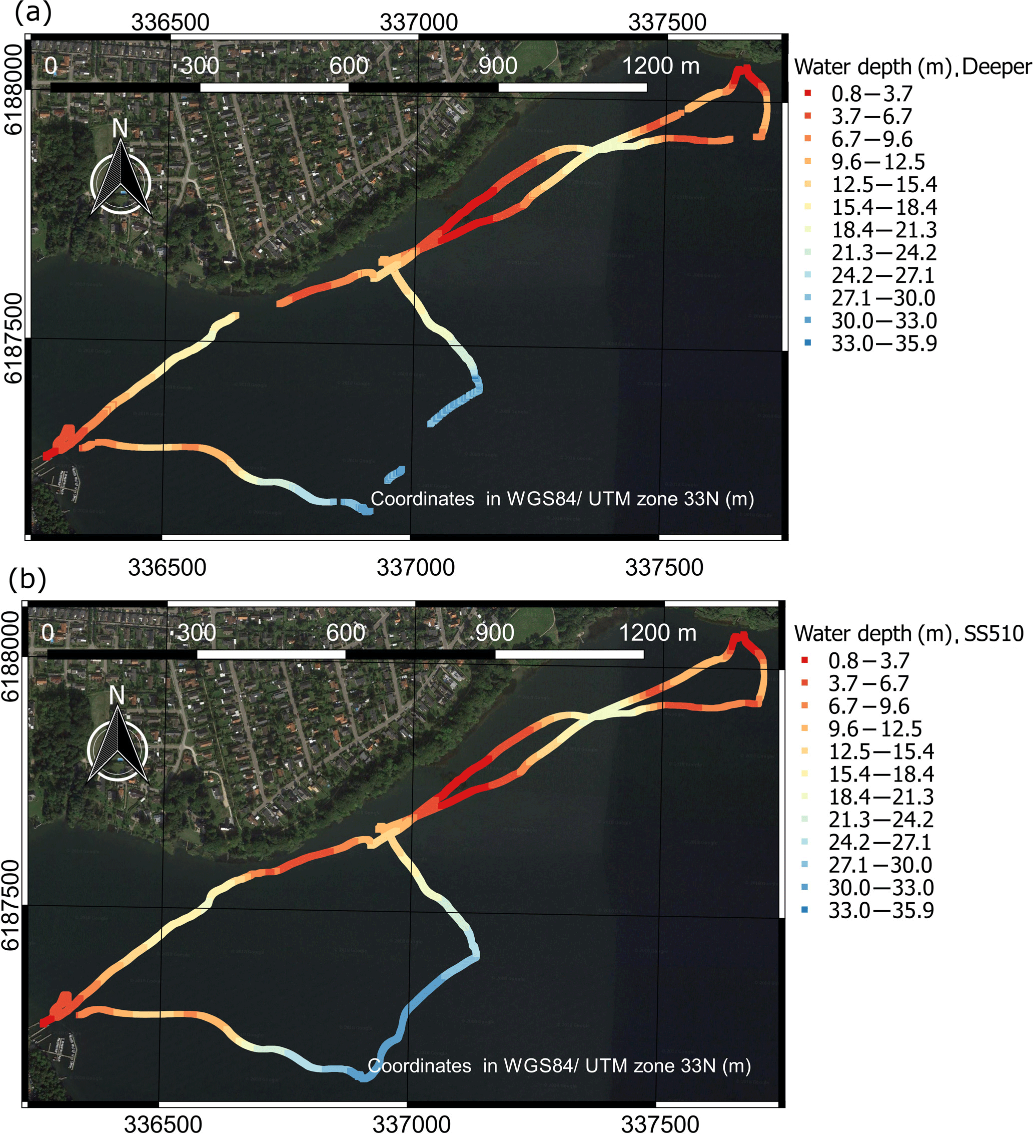
Figure 6Water depth measurements retrieved in Furesø by the two sonars: (a) observations with Deeper sonar; (b) observations with SS510 sonar.
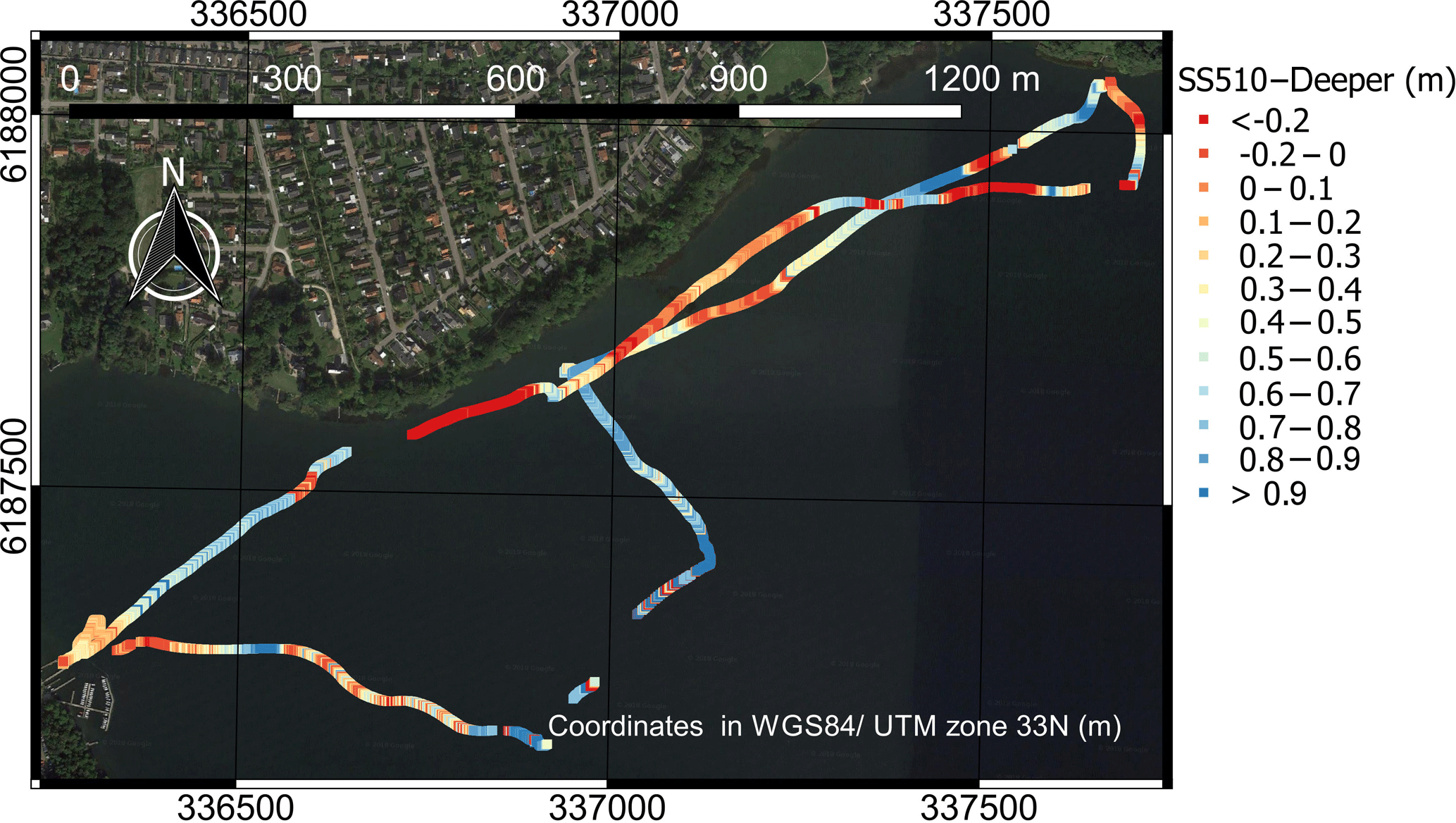
The maximum water depth retrieved during the survey is ∼36 m. In Fig. 7, we report the difference between the observations retrieved by the SS510 and the Deeper sonar.
Table 1Statistics comparing the Deeper sonar, SS510 sonar, and ground truth observations.
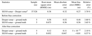
∗ Statistics computed after removing outliers (above the 95th percentile and below the 5th percentile).

Figure 7 shows high consistency between the two sonars. However, littoral areas with dense submerged vegetation show larger errors. While in the deepest area (∼30 m deep) the Deeper sonar observed multiple returns of the sound wave caused by suspended sediments, the analysis of the waveform was more complicated and subject to errors. In this area, the Deeper sonar fails to retrieve some water depth observations, where the waveform analysis does not show a well-defined strong return echo.
The observations retrieved by the two sonars are compared with ground truth observations in Fig. 8.
Figure 8 depicts a systematic overestimation of water depth by both sensors. The relationship between the observations of the two sonar sensors (x) and ground truth (y) can be described with a linear regression of the form shown in Eq. (10), in which β0 is the offset (y intercept), β1 is the slope, and ε is a random error term:
This survey showed an offset of zero. Thus, the bias between the ground truth observations and the sonar observations can be corrected by multiplying the sonar observations by β1. Linear regression lines can be fitted to the observations shown in Fig. 8 with a R2 of ∼0.99. Appendix A shortly describes how physical variables (such as depth, salinity, and temperature) can affect water depth observations using sonars.
Table 1 shows comparative statistics between the Deeper, the SS510 sonar, and the ground truth observations.
Table 1 shows a difference of ∼30 cm between the measurements of the two sonars, with the Deeper sonar generally underestimating water depth. This can be due to the wider scanning angle of the Deeper (15∘) compared to the SS510 sonar (9∘). The Deeper sonar is more affected by steep slopes, in which the depth tends to represent the most shallow point in the beam because of the larger scanning angle. The Deeper and SS510 observations can be corrected multiplying by the slope β1 (∼0.97 for the Deeper and ∼0.96 for the SS510 sonar). The correction factor is site specific as it depends on the bed form and material, as well as on the water properties (temperature, salinity, and pressure). Therefore, the acquisition of a sample of ground control points is required.
3.2 UAV-borne measurements
In Fig. 9 we show the observations of the UAV-borne survey above Furesø.
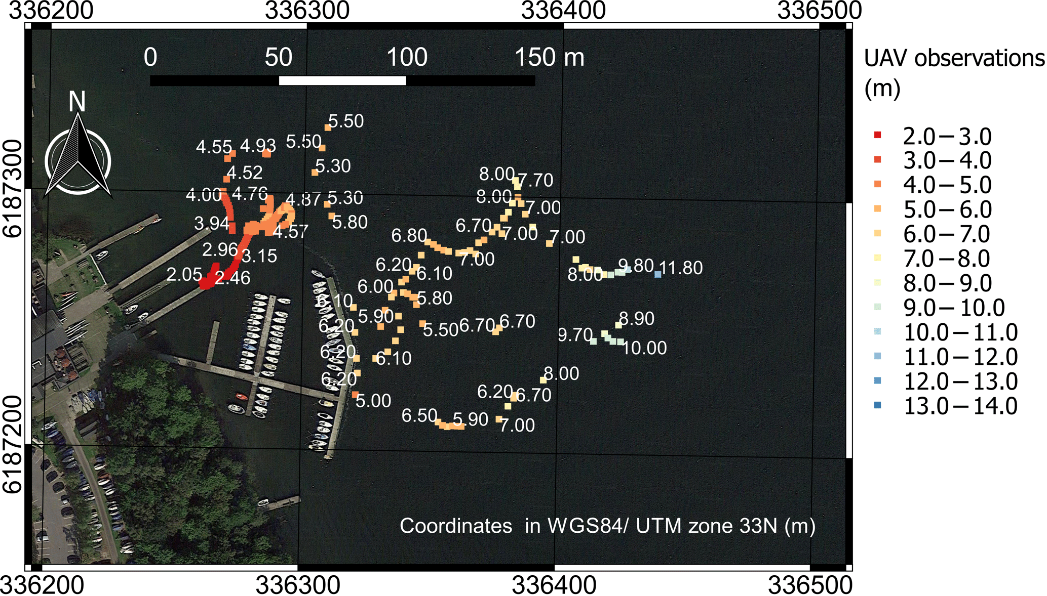
Figure 9Water depth (m) observations retrieved in Furesø with the the sonar tethered to the UAV.
Figure 10 depicts the UAV observations of four different cross sections of Marrebæk Kanal.
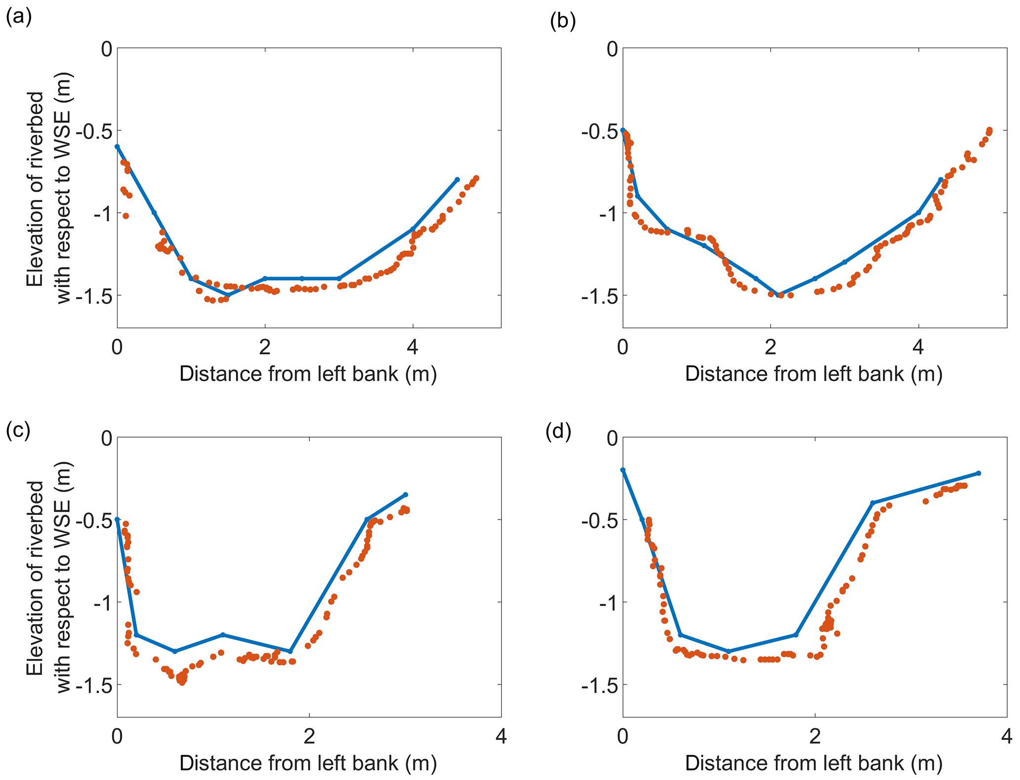
Figure 10River cross sections retrieved at different locations along Marrebæk Kanal. The y axis shows the difference between riverbed elevation and WSE (opposite sign of water depth). Red points are retrieved with UAV-borne observations and blue lines are the ground truth observations. The latitude and longitude coordinates of the left bank of the river cross sections are (a) 54.676300, 11.913296∘; (b) 54.675507, 11.913628∘; (c) 54.682117, 11.911957∘; and (d) 54.681779, 11.910723∘ (WGS84 reference system).
The accuracy of ground truth observations depends on both (i) the accuracy of the GNSS observations and (ii) the accuracy in positioning the GNSS pole in contact with the river bed. A vertical accuracy of ∼5–7 cm and a horizontal accuracy of ∼2–3 cm are estimated for the RTK GNSS ground truth observations, while the accuracy of the UAV-borne river-cross-section observations depends on (i) the error in absolute position of the sonar and (ii) the sonar's accuracy in measuring depth. The Deeper sonar shows a systematic overestimation of water depth in Fig. 10, which can be corrected by multiplying by the slope coefficient (β1∼0.95 for this specific survey). Figure 11 shows the observations after correction for the measurement bias.
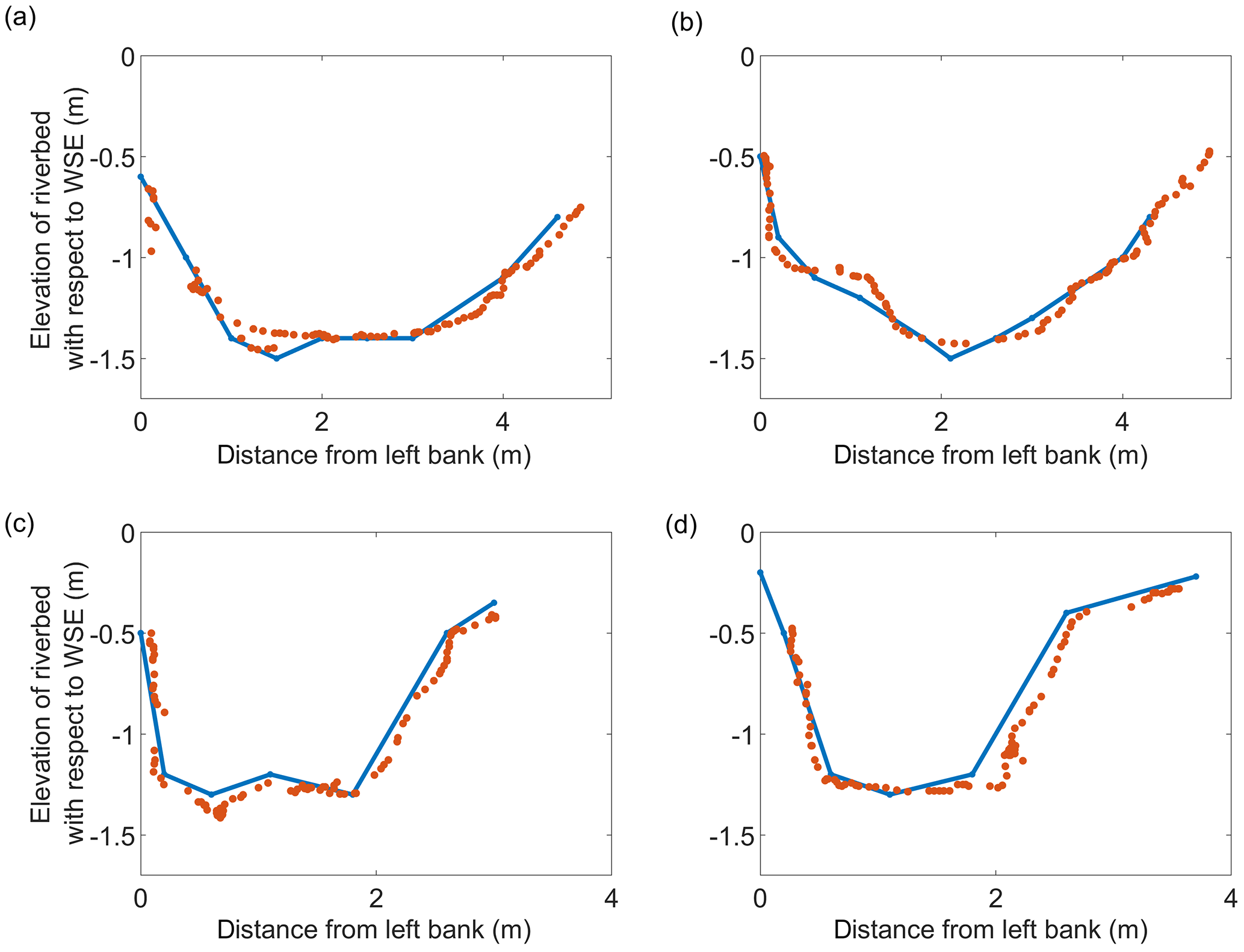
Figure 11River-cross-section observations retrieved from Marrebæk Kanal at the locations shown in Fig. 10 after bias correction of the Deeper sonar observations. Red points are retrieved with UAV-borne observations and blue lines are the ground truth observations.
UAV-borne bathymetric surveys provide high spatial resolution. Surveys can be interpolated to obtain bathymetric maps of entire river stretches. Figure 12 shows UAV observations in Åmose Å retrieved with the Deeper sonar at a resolution of ∼0.5 m. These observations were interpolated using the triangulated irregular network method. Two ground truth cross sections were retrieved with the RTK GNSS rover. The investigated stretch of Åmose Å has a length of ∼85 m and a maximum water depth of ∼1.15 m.
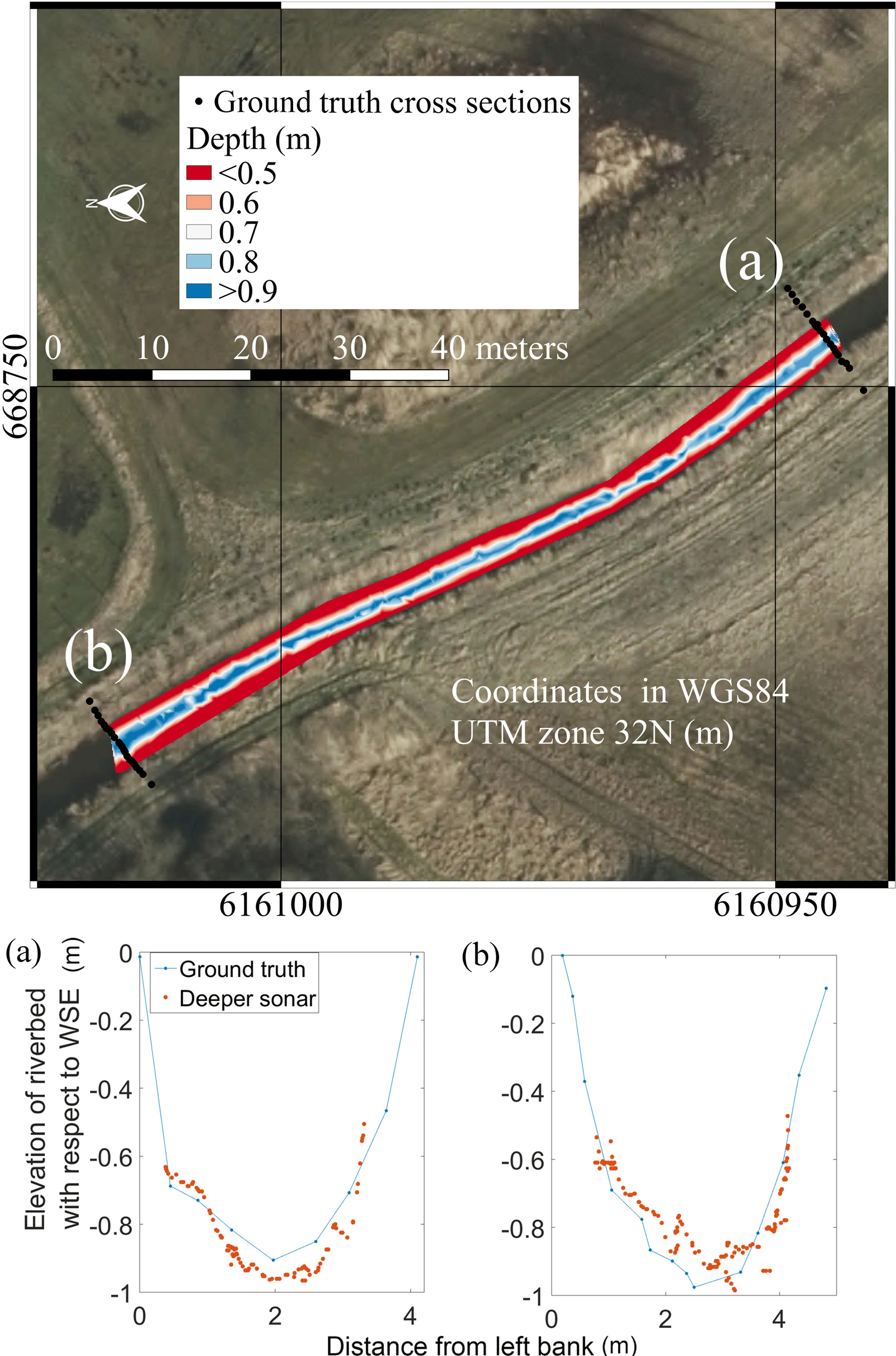
Figure 12Bathymetry observations in Åmose Å. Top panel shows the surveyed river stretch (north direction pointing towards the left side of the map as indicated by the north arrow). Background map is an airborne orthophoto provided by the Danish Styrelsen for Dataforsyning og Effektivisering (https://kortforsyningen.dk/, last access: 6 September 2017). Raster foreground map shows UAV-borne observations interpolated with the triangulated irregular network method. Two ground truth cross sections were retrieved, which are shown in the bottom panels: (a) upstream and (b) downstream cross section. In the cross section plots, the x axis shows the distance from left bank (west bank), and the y axis shows the difference between riverbed elevation and WSE (opposite sign of water depth).
Figure 12 shows that the minimum depth restriction is a significant limitation of the Deeper sonar in small rivers and streams. Water depth values smaller than ∼0.5 m are generally not measured by the Deeper sonar. Furthermore, the soft sediment and the submerged vegetation cause significant errors in the Deeper observations when compared to ground truth cross sections. In this survey, it was not possible to identify a systematic error and thus correct for the bias of the UAV-borne observations.
3.3 Accuracy of the Deeper sonar position
The accuracy of the absolute position of the Deeper sonar depends on the accuracy of (i) the drone horizontal position, (ii) the drone heading, and (iii) the relative position of the sonar with respect to the drone. The accuracies of these observations are reported in Table 2.
The accuracy of the relative position of the sonar depends on the image analysis procedure implemented to convert an offset from pixel into metric units. This procedure is also affected by the accuracy of the radar-derived WSE, because OD is an input to Eqs. (1) and (2). Tests were conducted in static mode using a checkerboard, placed at a series of known distances between 1 and 4 m, to evaluate the accuracy of measuring true distances in the image. These experiments showed that the offset between the camera and the sensor could be determined with an accuracy of 3 % of its actual value. The error in the conversion from image units to true distance units is mainly due to the (i) uncorrected lens distortion and (ii) assumption, made in Eqs. (1) and (2), that focal length is precisely known and that the distance between the rear nodal point of the lens and the image plane is exactly equal to focal length.
Table 2Accuracy of the different sensors used to measure the absolute position of the sonar.
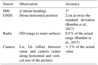
An error propagation study evaluated the overall accuracy of the absolute position of the sonar in real-world horizontal coordinates. For detailed information, see the data in the Supplement. The uncertainties of β, Lw, and Lh have the larger impact on the overall accuracy, compared to other error sources, such as OD and drone horizontal position. Since the offset (L) between the center of the camera and the sonar typically assumes values between 0 and 2 m, the overall accuracy of the Deeper sonar position is generally better than 20 cm. This accuracy is acceptable for most bathymetric surveys, particularly in light of the spatial resolution (15∘ beam divergence) of the Deeper sonar measurements.
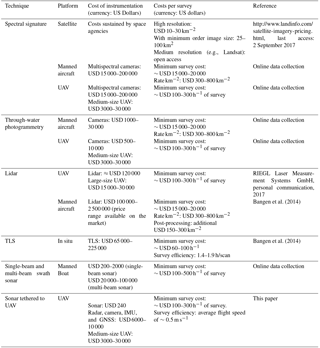
Bathymetry can be measured with both in situ and remote sensing methods. In situ methods generally deploy bathymetric sonars installed on vessels. Remote sensing methods include (i) lidar techniques, (ii) methods evaluating the relationship between spectral signature and depth, and (iii) through-water photogrammetry. Remote sensing methods generally allow for larger spatial coverage than in situ methods, but only shallow and clear water bodies can be surveyed. Table 3 shows a comparison of the different remote sensing and in situ techniques. UAV-borne sonar depth measurements bridge the gap between ground surveys and remote sensing techniques. The deployed Deeper sonar can measure deep and turbid water, and reach remote and dangerous areas, including unnavigable streams, when it is tethered to UAV. For depths up to ∼30 m, the 2.1 % accuracy complies with the first accuracy level established by the International Hydrographic Organization (IHO) for accurate bathymetric surveys. Indeed, for depths of 30 m, the accuracy of the tethered sonar is ∼0.630 m, while the first IHO level standard requires an accuracy better than 0.634 m. Conversely, for depths greater than 30 m, the UAV-borne sonar measurements comply with the second IHO level. Because of the large beam angle of the Deeper sonar, small-scale bathymetric features at greater depth cannot be resolved. However, a large beam angle (e.g., 8–30∘) is an intrinsic limitation of single-beam sonar systems. For these reasons, when detection of small-scale features is required, surveys are generally performed with vessels equipped with multi-beam swath systems or side-scan imaging sonars. These systems are significantly more expensive, heavier, and larger than single-beam sonars, which makes integration with UAV platforms difficult.
Table 3Comparison of different approaches for measuring river bathymetry.
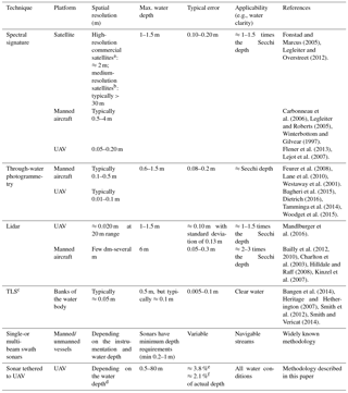
a Multispectral bands: IKONOS, QuickBird, and WorldView-2. b Landsat. c Terrestrial laser scanner (TLS). d The divergence of the sonar cone beam is 15∘. e Before bias correction. f After bias correction.
Table 3 does not include methods requiring the operator to wade into a river, e.g., measurements taken with a RTK GNSS rover (e.g., Bangen et al., 2014). To take measurements with a GNSS rover, the operator must submerge the antenna pole until it reaches the river bed surface. Therefore, this method can only be used for local observations. Furthermore, innovative approaches such as using a ground penetrating radar (GPR) are not included because they are still at the level of local proof-of-concept applications (Costa et al., 2000; Spicer et al., 1997) and generally require cableways to suspend instrumentation a few decimeters above the water surface.
In order to obtain reliable measurements and ensure effective post-processing of the data, the techniques shown in Table 3 require initial expenditure and expertise from multiple fields, e.g., electric and software engineers (for technology development and data analysis), pilots (e.g., UAVs and manned aircrafts), experts in river navigation (for boats), surveyors (e.g., for GNSS rovers, photogrammetry), hydrologists, and geologists. In Appendix B, the typical survey expenditures for the different techniques are shown.
Future research
UAV-borne measurements of water depth have the potential to enrich the set of available hydrological observations. Their advantages compared to airborne, satellite, and manned boat measurements were demonstrated in this study. The competitiveness of UAVs in measuring water depth, compared to the capabilities of unmanned aquatic vessels equipped with sonar and RTK GNSS systems, is currently limited to water bodies that do not allow navigation of unmanned aquatic vessels, e.g., because of high water currents, slopes, or obstacles. The full potential of UAV-borne hydrological observations will be exploited only with flight operations beyond visual line of sight. The new generation of waterproof rotary wing UAVs equipped with visual navigation sensors and automatic pilot systems will make it possible to collect hyperspatial observations in remote or dangerous locations, without requiring the operator to access the area.
UAVs are flexible and low-cost platforms. UAVs allow operators to retrieve hyperspatial hydrological observations with high spatial and temporal resolution. Automatic flight, together with computer vision navigation, allows UAVs to monitor dangerous or remote areas, including unnavigable streams.
This study shows how water depths can be retrieved by a tethered sonar controlled by UAVs. In particular, we highlighted the following:
-
The accuracy of the measured water depth is not significantly affected by bottom structure and water turbidity if the sound waveform is correctly processed. However, submerged vegetation and soft sediments can affect sonar observations.
-
Observations were retrieved for water depths ranging from 0.5 up to 35 m. Accuracy can be improved from ∼3.8 % to ∼2.1 % after correction of the observational bias, which can be identified and quantified by acquiring a representative sample of ground truth observations. The observational bias, which was observed in most experiments, can be caused by the dependence of the sound wave speed on temperature, salinity, and pressure. The relatively wide beam angle (15∘) of the UAV-tethered sonar implies coarse spatial resolution, especially at large water depths, and limits the detection of small-scale differences in depth.
-
The accuracy and maximum survey depth achieved in this study exceed those of any other remote sensing techniques and are comparable with bathymetric sonars transported by manned or unmanned aquatic vessels.
Datasets used in the study are available online in the repository archived in Zenodo.org, https://doi.org/10.5281/zenodo.1309416 (Bandini et al., 2018). The repository contains MATLAB datasets, scripts, together with vector and raster files that can be used to replicate the figures of this paper.
In Fig. 8 the measurements of the two different sonars lie along a line with a nearly constant slope (not coincident with the 1:1 line) with respect to the ground truth observations.
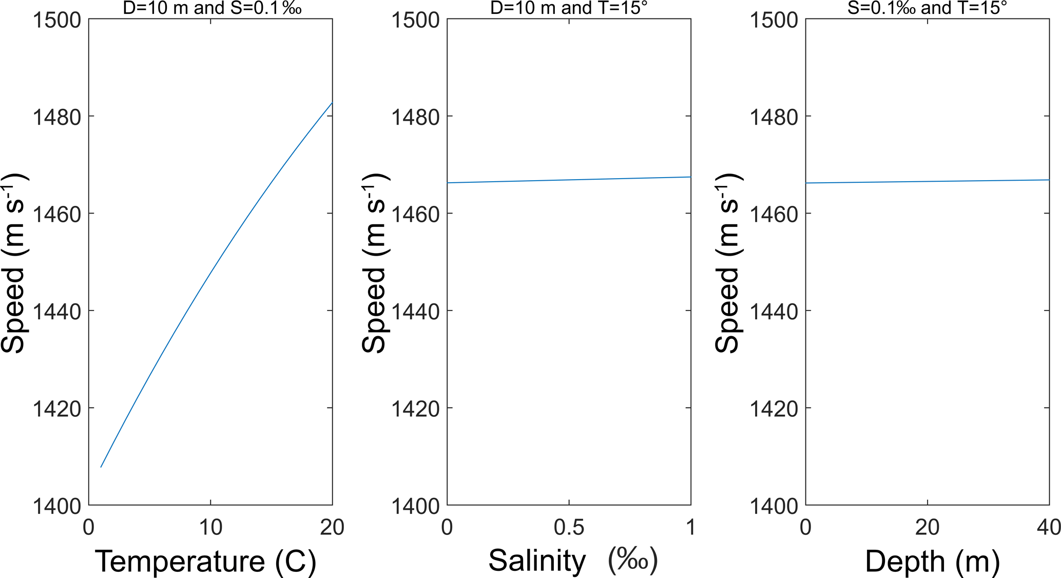
The equation presented by Chen and Millero (1977) is the international standard algorithm, often known as the UNESCO algorithm, that computes the speed of sound (c) in water as a complex function of temperature (T), salinity (S), and pressure (P).
This equation has a range of validity: temperature 0 to 40 ∘C, salinity 0 to 40 parts per thousand, pressure 0 to 1000 bar (Wong and Zhu, 1995). Measurements were conducted in the Furesø lake, which has a salinity of less than 0.5 ‰, a recorded surface temperature between 12 and 19∘, and a depth up to ∼35 m. A sensitivity analysis with one factor varying at the time was applied to the Chen and Millero equation to estimate the range of variability of the speed of sound at different temperature, salinity, and depth (or pressure) values, as shown in Fig. A1.
As shown Fig. A1, temperature has the largest influence on speed of sound. Thus, the slope of linear regression between sonar and ground truth measurements is mainly determined by the temperature profiles and only to a lesser extent by the salinity and depth. Indeed, although the two sonars measure the surface temperature of water, no internal compensation is performed for the vertical temperature profile.
Costs related to the individual approaches to measure bathymetry are difficult to estimate and compare. Costs include an initial expenditure and additional expenses depending on the nature of each survey. These typically depend on the duration of the survey, on the size of the area to be surveyed, on the needed accuracy and resolution, on the cost of labor, and on the water body characteristics. Table B1 compares the approximate costs for the techniques that are most commonly used to retrieve water depth.
The supplement related to this article is available online at: https://doi.org/10.5194/hess-22-4165-2018-supplement.
The authors declare that they have no conflict of interest.
Ole Smith, Thyge Bjerregaard Pedersen, Karsten Stæhr Hansen, and Mikkel Lund Schmedes from Orbicon A/S provided help and technical support during the bathymetric surveys.
The Innovation Fund Denmark is acknowledged for providing funding for this
study via the project Smart UAV (125-2013-5).
Edited by: Anas Ghadouani
Reviewed by: two anonymous referees
Alsdorf, D. E., Rodriguez, E., and Lettenmaier, D. P.: Measuring surface water from space, Rev. Geophys., 45, 1–24, https://doi.org/10.1029/2006RG000197, 2007.
Bagheri, O., Ghodsian, M., and Saadatseresht, M.: Reach scale application of UAV+SfM method in shallow rivers hyperspatial bathymetry, Int. Arch. Photogramm., 40, 77–81, 2015.
Bailly, J.-S., Kinzel, P. J., Allouis, T., Feurer, D., and Le Coarer, Y.: Airborne LiDAR Methods Applied to Riverine Environments, in: Fluvial Remote Sensing for Science and Management, edited by: Carbonneau, P. E. and Piégay, H., 141–161, 2012.
Bailly, J. S., le Coarer, Y., Languille, P., Stigermark, C. J., and Allouis, T.: Geostatistical estimations of bathymetric LiDAR errors on rivers, Earth Surf. Proc. Land., 35, 1199–1210, https://doi.org/10.1002/esp.1991, 2010.
Bandini, F., Jakobsen, J., Olesen, D., Reyna-Gutierrez, J. A., and Bauer-Gottwein, P.: Measuring water level in rivers and lakes from lightweight Unmanned Aerial Vehicles, J. Hydrol., 548, 237–250, https://doi.org/10.1016/j.jhydrol.2017.02.038, 2017.
Bandini, F., Olesen, D., Jakobsen, J., Kittel, C. M. M., Wang, S., Garcia, M., and Bauer-Gottwein, P.: Dataset used in “Bathymetry observations of inland water bodies using a tethered single-beam sonar controlled by an Unmanned Aerial Vehicle” (https://doi.org/10.5194/hess-2017-625), https://doi.org/10.5281/ZENODO.1309417, 2018.
Bangen, S. G., Wheaton, J. M., Bouwes, N., Bouwes, B., and Jordan, C.: A methodological intercomparison of topographic survey techniques for characterizing wadeable streams and rivers, Geomorphology, 206, 343–361, https://doi.org/10.1016/j.geomorph.2013.10.010, 2014.
Brown, C. J. and Blondel, P.: Developments in the application of multibeam sonar backscatter for seafloor habitat mapping, Appl. Acoust., 70, 1242–1247, https://doi.org/10.1016/j.apacoust.2008.08.004, 2009.
Brown, D. C.: Close-range camera calibration, Photogramm. Eng., 37, 855–866, 1971.
Brown, H. C., Jenkins, L. K., Meadows, G. A., and Shuchman, R. A.: BathyBoat: An autonomous surface vessel for stand-alone survey and underwater vehicle network supervision, Mar. Technol. Soc. J., 44, 20–29, 2010.
Carbonneau, P. E., Lane, S. N., and Bergeron, N.: Feature based image processing methods applied to bathymetric measurements from airborne remote sensing in fluvial environments, Earth Surf. Proc. Land., 31, 1413–1423, https://doi.org/10.1002/esp.1341, 2006.
Charlton, M. E., Large, A. R. G., and Fuller, I. C.: Application of airborne lidar in river environments: The River Coquet, Northumberland, UK, Earth Surf. Proc. Land., 28, 299–306, https://doi.org/10.1002/esp.482, 2003.
Chen, C. and Millero, F. J.: Speed of sound in seawater at high pressures, J. Acoust. Soc. Am., 62, 1129–1135, https://doi.org/10.1121/1.381646, 1977.
Clarke, T. and Fryer, J.: The development of camera calibration methods and models, Photogramm. Rec., 16, 51–66, https://doi.org/10.1111/0031-868X.00113, 1998.
Conner, J. T. and Tonina, D.: Effect of cross-section interpolated bathymetry on 2D hydrodynamic model results in a large river, Earth Surf. Proc. Land., 39, 463–475, https://doi.org/10.1002/esp.3458, 2014.
Costa, J. E., Spicer, K. R., Cheng, R. T., Haeni, F. P., Melcher, N. B., Thurman, E. M., Plant, W. J., and Keller, W. C.: Measuring stream discharge by non-contact methods: A proof-of-concept experiment, Geophys. Res. Lett., 27, 553–556, https://doi.org/10.1029/1999GL006087, 2000.
Detert, M. and Weitbrecht, V.: A low-cost airborne velocimetry system: proof of concept, J. Hydraul. Res., 53, 532–539, https://doi.org/10.1080/00221686.2015.1054322, 2015.
Dietrich, J. T.: Bathymetric Structure from Motion: Extracting shallow stream bathymetry from multi-view stereo photogrammetry, Earth Surf. Proc. Land., 42, 355–364, https://doi.org/10.1002/esp.4060, 2016.
Faig, W.: Calibration of close-range photogrammetry systems: Mathematical formulation, Photogramm. Eng. Rem. S., 41, 1479–1486, 1975.
Ferreira, H., Almeida, C., Martins, A., Almeida, J., Dias, N., Dias, A., and Silva, E.: Autonomous bathymetry for risk assessment with ROAZ robotic surface vehicle, in OCEANS '09 IEEE, Bremen, 2009.
Feurer, D., Bailly, J.-S., Puech, C., Le Coarer, Y., and Viau, A. A.: Very-high-resolution mapping of river-immersed topography by remote sensing, Prog. Phys. Geogr., 32, 403–419, https://doi.org/10.1177/0309133308096030, 2008.
Flener, C., Vaaja, M., Jaakkola, A., Krooks, A., Kaartinen, H., Kukko, A., Kasvi, E., Hyyppä, H., Hyyppä, J., and Alho, P.: Seamless mapping of river channels at high resolution using mobile liDAR and UAV-photography, Remote Sens., 5, 6382–6407, https://doi.org/10.3390/rs5126382, 2013.
Fonstad, M. A. and Marcus, W. A.: Remote sensing of stream depths with hydraulically assisted bathymetry (HAB) models, Geomorphology, 72, 320–339, https://doi.org/10.1016/j.geomorph.2005.06.005, 2005.
Gichamo, T. Z., Popescu, I., Jonoski, A., and Solomatine, D.: River cross-section extraction from the ASTER global DEM for flood modeling, Environ. Model. Softw., 31, 37–46, https://doi.org/10.1016/j.envsoft.2011.12.003, 2012.
Giordano, F., Mattei, G., Parente, C., Peluso, F., and Santamaria, R.: Integrating sensors into a marine drone for bathymetric 3D surveys in shallow waters, Sensors, 16, 41, https://doi.org/10.3390/s16010041, 2015.
Guenther, G. C.: Airborne Lidar Bathymetry, in Digital Elevation Model Technologies and Applications, The DEM Users Manual, 253–320, 8401 Arlington Blvd., 2001.
Guenther, G. C., Cunningham, A. G., Larocque, P. E., Reid, D. J., Service, N. O., Highway, E., and Spring, S.: Meeting the Accuracy Challenge in Airborne Lidar Bathymetry, EARSeL eProceedings, 1, 1–27, 2000.
Hamylton, S., Hedley, J., and Beaman, R.: Derivation of High-Resolution Bathymetry from Multispectral Satellite Imagery: A Comparison of Empirical and Optimisation Methods through Geographical Error Analysis, Remote Sens., 7, 16257–16273, https://doi.org/10.3390/rs71215829, 2015.
Heritage, G. L. and Hetherington, D.: Towards a protocol for laser scanning in fluvial geomorphology, Earth Surf. Proc. Land., 32, 66–74, https://doi.org/10.1002/esp.1375, 2007.
Hilldale, R. C. and Raff, D.: Assessing the ability of airborne LiDAR to map river bathymetry, Earth Surf. Proc. Land., 33, 773–783, https://doi.org/10.1002/esp.1575, 2008.
Kinzel, P. J., Wright, C. W., Nelson, J. M., and Burman, A. R.: Evaluation of an Experimental LiDAR for Surveying a Shallow, Braided, Sand-Bedded River, J. Hydraul. Eng., 133, 838–842, https://doi.org/10.1061/(ASCE)0733-9429(2007)133:7(838), 2007.
Lane, S. N., Widdison, P. E., Thomas, R. E., Ashworth, P. J., Best, J. L., Lunt, I. A., Sambrook Smith, G. H., and Simpson, C. J.: Quantification of braided river channel change using archival digital image analysis, Earth Surf. Proc. Land., 35, 971–985, https://doi.org/10.1002/esp.2015, 2010.
Lee, K. R., Kim, A. M., Olsen;, R. C., and Kruse, F. A.: Using WorldView-2 to determine bottom-type and bathymetry, Proc. SPIE 8030, Ocean Sensing and Monitoring III, , 80300D (5 May 2011), vol. 2, 2011.
Legleiter, C. J.: Remote measurement of river morphology via fusion of LiDAR topography and spectrally based bathymetry, Earth Surf. Proc. Land., 37, 499–518, https://doi.org/10.1002/esp.2262, 2012.
Legleiter, C. J. and Overstreet, B. T.: Mapping gravel bed river bathymetry from space, J. Geophys. Res.-Earth, 117, https://doi.org/10.1029/2012JF002539, 2012.
Legleiter, C. J. and Roberts, D. A.: Effects of channel morphology and sensor spatial resolution on image-derived depth estimates, Remote Sens. Environ., 95, 231–247, https://doi.org/10.1016/j.rse.2004.12.013, 2005.
Legleiter, C. J., Roberts, D. A., and Lawrence, R. L.: Spectrally based remote sensing of river bathymetry, Earth Surf. Proc. Land., 34, 1039–1059, https://doi.org/10.1002/esp.1787, 2009.
Lejot, J., Delacourt, C., Piégay, H., Fournier, T., Trémélo, M.-L., and Allemand, P.: Very high spatial resolution imagery for channel bathymetry and topography from an unmanned mapping controlled platform, Earth Surf. Proc. Land., 32, 1705–1725, https://doi.org/10.1002/esp.1595, 2007.
Liceaga-Correa, M. A. and Euan-Avila, J. I.: Assessment of coral reef bathymetric mapping using visible Landsat Thematic Mapper data, Int. J. Remote Sens., 23, 3–14, https://doi.org/10.1080/01431160010008573, 2002.
Lyons, M., Phinn, S., and Roelfsema, C.: Integrating Quickbird multi-spectral satellite and field data: Mapping bathymetry, seagrass cover, seagrass species and change in Moreton Bay, Australia in 2004 and 2007, Remote Sens., 3, 42–64, https://doi.org/10.3390/rs3010042, 2011.
Lyzenga, D. R.: Remote sensing of bottom reflectance and water attenuation parameters in shallow water using aircraft and Landsat data, Int. J. Remote Sens., 2, 71–82, https://doi.org/10.1080/01431168108948342, 1981.
Lyzenga, D. R., Malinas, N. P., and Tanis, F. J.: Multispectral bathymetry using a simple physically based algorithm, IEEE Trans. Geosci. Remote Sens., 44, 2251–2259, https://doi.org/10.1109/TGRS.2006.872909, 2006.
Mandlburger, G., Pfennigbauer, M., Wieser, M., Riegl, U., and Pfeifer, N.: Evaluation Of A Novel Uav-Borne Topo-Bathymetric Laser Profiler, ISPRS – Int. Arch. Photogramm. Remote Sens. Spat. Inf. Sci., XLI-B1, 933–939, https://doi.org/10.5194/isprs-archives-XLI-B1-933-2016, 2016.
Manley, P. L. and Singer, J. K.: Assessment of sedimentation processes determined from side-scan sonar surveys in the Buffalo River, New York, USA, Environ. Geol., 55, 1587–1599, https://doi.org/10.1007/s00254-007-1109-8, 2008.
Marcus, W. A., Legleiter, C. J., Aspinall, R. J., Boardman, J. W., and Crabtree, R. L.: High spatial resolution hyperspectral mapping of in-stream habitats, depths, and woody debris in mountain streams, Geomorphology, 55, 363–380, https://doi.org/10.1016/S0169-555X(03)00150-8, 2003.
Nitsche, F. O., Ryan, W. B. F., Carbotte, S. M., Bell, R. E., Slagle, A., Bertinado, C., Flood, R., Kenna, T., and McHugh, C.: Regional patterns and local variations of sediment distribution in the Hudson River Estuary, Estuar. Coast. Shelf Sci., 71, 259–277, https://doi.org/10.1016/j.ecss.2006.07.021, 2007.
Overstreet, B. T. and Legleiter, C. J.: Removing sun glint from optical remote sensing images of shallow rivers, Earth Surf. Proc. Land., 42, 318–333, 2017.
Powers, J., Brewer, S. K., Long, J. M., and Campbell, T.: Evaluating the use of side-scan sonar for detecting freshwater mussel beds in turbid river environments, Hydrobiologia, 743, 127–137, https://doi.org/10.1007/s10750-014-2017-z, 2015.
Ridolfi, E. and Manciola, P.: Water level measurements from drones: A Pilot case study at a dam site, Water (Switzerland), https://doi.org/10.3390/w10030297, 2018.
Rovira, A., Batalla, R. J., and Sala, M.: Fluvial sediment budget of a Mediterranean river: The lower Tordera (Catalan Coastal Ranges, NE Spain), Catena, 60, 19–42, https://doi.org/10.1016/j.catena.2004.11.001, 2005.
Schäppi, B., Perona, P., Schneider, P., and Burlando, P.: Integrating river cross section measurements with digital terrain models for improved flow modelling applications, Comput. Geosci., 36, 707–716, https://doi.org/10.1016/j.cageo.2009.12.004, 2010.
Smith, M., Vericat, D., and Gibbins, C.: Through-water terrestrial laser scanning of gravel beds at the patch scale, Earth Surf. Proc. Land., 37, 411–421, https://doi.org/10.1002/esp.2254, 2012.
Smith, M. W. and Vericat, D.: Evaluating shallow-water bathymetry from through-water terrestrial laser scanning under a range of hydraulic and physical water quality conditions, River Res. Appl., 30, 905–924, https://doi.org/10.1002/rra.2687, 2014.
Snellen, M., Siemes, K., and Simons, D. G.: Model-based sediment classification using single-beam echosounder signals., J. Acoust. Soc. Am., 129, 2878–2888, https://doi.org/10.1121/1.3569718, 2011.
Spicer, K. R., Costa, J. E., and Placzek, G.: Measuring flood discharge in unstable stream channels using ground-penetrating radar, Geology, 25, 423–426, https://doi.org/10.1130/0091-7613(1997)025<0423:MFDIUS>2.3.CO;2, 1997.
Strayer, D. L., Malcom, H. M., Bell, R. E., Carbotte, S. M., and Nitsche, F. O.: Using geophysical information to define benthic habitats in a large river, Freshw. Biol., 51, 25–38, https://doi.org/10.1111/j.1365-2427.2005.01472.x, 2006.
Stumpf, R. P., Holderied, K., and Sinclair, M.: Determination of water depth with high-resolution satellite imagery over variable bottom types, Limnol. Oceanogr., 48, 547–556, https://doi.org/10.4319/lo.2003.48.1_part_2.0547, 2003.
Tamminga, A., Hugenholtz, C., Eaton, B., and Lapointe, M.: Hyperspatial Remote Sensing of Channel Reach Morphology and Hydraulic Fish Habitat Using an Unmanned Aerial Vehicle (Uav): a First Assessment in the Context of River Research and Management, River Res. Appl., 31, 379–391, https://doi.org/10.1002/rra.2743, 2014.
Tauro, F., Petroselli, A., and Arcangeletti, E.: Assessment of drone-based surface flow observations, Hydrol. Process., 30, 1114–1130, https://doi.org/10.1002/hyp.10698, 2015a.
Tauro, F., Pagano, C., Phamduy, P., Grimaldi, S., and Porfiri, M.: Large-Scale Particle Image Velocimetry From an Unmanned Aerial Vehicle, IEEE/ASME Trans. Mechantronics, 20, 1–7, https://doi.org/10.1109/TMECH.2015.2408112, 2015b.
Tauro, F., Porfiri, M., and Grimaldi, S.: Surface flow measurements from drones, J. Hydrol., 540, 240–245, https://doi.org/10.1016/j.jhydrol.2016.06.012, 2016.
Virili, M., Valigi, P., Ciarfuglia, T., and Pagnottelli, S.: A prototype of radar-drone system for measuring the surface flow velocity at river sites and discharge estimation, Geophys. Res. Abstr., 17, 2015–12853, 2015.
Walker, D. J. and Alford, J. B.: Mapping Lake Sturgeon Spawning Habitat in the Upper Tennessee River using Side-Scan Sonar, North Am. J. Fish. Manag., 36, 1097–1105, https://doi.org/10.1080/02755947.2016.1198289, 2016.
Weng, J., Coher, P., and Herniou, M.: Camera Calibration with Distortion Models and Accuracy Evaluation, IEEE T. Pattern Anal., 14, 965–980, https://doi.org/10.1109/34.159901, 1992.
Westaway, R. M., Lane, S. N., and Hicks, D. M.: Remote sensing of clear-water, shallow, gravel-bed rivers using digital photogrammetry, Photogramm. Eng. Rem. S., 67, 1271–1281, 2001.
Winterbottom, S. J. and Gilvear, D. J.: Quantification of channel bed morphology in gravel-bed rivers using airborne multispectral imagery and aerial photography, Regul. Rivers-Research Manag., 13, 489–499, https://doi.org/10.1002/(SICI)1099-1646(199711/12)13:6<489::AID-RRR471>3.0.CO;2-X, 1997.
Wong, G. S. K. and Zhu, S.: Speed of sound in seawater as a function of salinity, temperature, and pressure, J. Acoust. Soc. Am., 97, 1732–1736, https://doi.org/10.1121/1.413048, 1995.
Woodget, A. S., Carbonneau, P. E., Visser, F., and Maddock, I. P.: Quantifying submerged fluvial topography using hyperspatial resolution UAS imagery and structure from motion photogrammetry, Earth Surf. Proc. Land., 40, 47–64, https://doi.org/10.1002/esp.3613, 2015.