the Creative Commons Attribution 4.0 License.
the Creative Commons Attribution 4.0 License.
 | 13 Aug 2018
Multi-source data assimilation for physically based hydrological modeling of an experimental hillslope
Anna Botto
Enrica Belluco
Matteo Camporese
Data assimilation has recently been the focus of much attention for integrated surface–subsurface hydrological models, whereby joint assimilation of water table, soil moisture, and river discharge measurements with the ensemble Kalman filter (EnKF) has been extensively applied. Although the EnKF has been specifically developed to deal with nonlinear models, integrated hydrological models based on the Richards equation still represent a challenge, due to strong nonlinearities that may significantly affect the filter performance. Thus, more studies are needed to investigate the capabilities of the EnKF to correct the system state and identify parameters in cases where the unsaturated zone dynamics are dominant, as well as to quantify possible tradeoffs associated with assimilation of multi-source data. Here, the CATHY (CATchment HYdrology) model is applied to reproduce the hydrological dynamics observed in an experimental two-layered hillslope, equipped with tensiometers, water content reflectometer probes, and tipping bucket flow gages to monitor the hillslope response to a series of artificial rainfall events. Pressure head, soil moisture, and subsurface outflow are assimilated with the EnKF in a number of scenarios and the challenges and issues arising from the assimilation of multi-source data in this real-world test case are discussed. Our results demonstrate that the EnKF is able to effectively correct states and parameters even in a real application characterized by strong nonlinearities. However, multi-source data assimilation may lead to significant tradeoffs: the assimilation of additional variables can lead to degradation of model predictions for other variables that are otherwise well reproduced. Furthermore, we show that integrated observations such as outflow discharge cannot compensate for the lack of well-distributed data in heterogeneous hillslopes.


Data assimilation, i.e., the process in which observations of a system are merged in a consistent manner with numerical model predictions (Moradkhani, 2008; Troch et al., 2003), has become increasingly popular in hydrological modeling over the last few decades (Montzka et al., 2012). Among the various techniques available, the ensemble Kalman filter (EnKF) (Evensen, 2003, 2009b) is probably the most widespread, thanks to its ease of implementation, capability to handle nonlinear models and potential to be used as a sequential inverse modeling tool when parameters are included in the update step. Applications in hydrology include studies in different disciplines, such as groundwater hydrology (Bailey and Baù, 2010; Chen and Zhang, 2006; Hendricks Franssen and Kinzelbach, 2008; Li et al., 2012; Zovi et al., 2017), rainfall–runoff modeling (Clark et al., 2008; Han and Li, 2008; Moradkhani et al., 2005; Vrugt et al., 2006; Weerts and El Serafy, 2006; Xie and Zhang, 2010), and land surface modeling at multiple scales (Cammalleri and Ciraolo, 2012; Crow and Wood, 2003; De Lannoy et al., 2007; Flores et al., 2012; Francois et al., 2003; Hain et al., 2012; Pan and Wood, 2006; Reichle et al., 2002a, b).
As a consequence of such popularity, the EnKF is also increasingly applied with integrated surface–subsurface hydrological models (IHSSMs), whereby multiple terrestrial compartments (e.g., snow cover, surface water, groundwater) are solved simultaneously, in an attempt to tackle environmental problems in a holistic approach (Kollet et al., 2017; Maxwell et al., 2014). For instance, Camporese et al. (2009a) and Camporese et al. (2009b) combined the CATHY model and the EnKF to assimilate pressure head, soil moisture, and streamflow data, finding that the assimilation of pressure head and soil moisture is beneficial to subsurface states and river discharge, but the assimilation of river discharge alone does not improve the prediction of subsurface states. Similar conclusions were drawn by Pasetto et al. (2012), who compared the EnKF with a modified particle filter to assimilate discharge and pressure head, using the CATHY model. More recently, Pasetto et al. (2015) used the EnKF and CATHY to investigate the impact of possible sensor failure on the observability of flow dynamics and estimation of the model parameters characterizing the soil properties of an artificial hillslope. Ridler et al. (2014) assimilated soil moisture remote sensing products in the MIKE SHE model and found that surface soil moisture has correction capabilities limited to the first 25 cm of soil. With the same model, Rasmussen et al. (2016), Rasmussen et al. (2015), Zhang et al. (2015), and Zhang et al. (2016) investigated in detail issues related to uncertainty quantification and biased observations, as well the impacts of update localization and ensemble size on the multivariate assimilation of groundwater head and river discharge at the catchment scale. Kurtz et al. (2015) first presented a data assimilation framework for the land surface–subsurface part of the Terrestrial System Modelling Platform (TerrSysMP), followed by Baatz et al. (2017), who assimilated distributed river discharge data into the TerrSysMP to estimate the spatially distributed Manning roughness coefficient, and Zhang et al. (2018), who tested and compared five data assimilation methodologies for assimilating groundwater level data via the EnKF to improve root zone soil moisture estimation. Within yet another modeling framework, Tang et al. (2017) used the EnKF in conjunction with HydroGeoSphere to study the influence of heterogeneous riverbeds on river–aquifer exchange fluxes.
In spite of such a strong interest, several issues related to the use of EnKF for state and parameter estimation in integrated hydrological modeling remain unresolved. The subsurface component of many IHSSMs is based on the solution of the Richards equation in one or three dimensions and, although recent studies with numerical experiments in synthetic test cases (Brandhorst et al., 2017; Erdal et al., 2014) have shown that the EnKF has great potential for the estimation of soil hydraulic parameters in the unsaturated zone, it is still unclear whether the method is able to cope with nonlinearities and parameter estimation in real test cases, where multiple uncertainties on initial and boundary conditions make the problem much more challenging (Bauser et al., 2016; De Lannoy et al., 2007; Monsivais-Huertero et al., 2010; Shi et al., 2015; Visser et al., 2006). Also, as more sources of data become available at cheaper cost, it is increasingly difficult to assess which data types are the most suitable or effective in assimilating and checking which possible tradeoffs might occur when assimilating different variables in a multivariate data assimilation framework. Zhang et al. (2018), for instance, found that joint assimilation of pressure head and soil moisture is beneficial only when pressure head is assimilated in the saturated zone and soil moisture in the unsaturated zone, while Zhang et al. (2016) showed that joint assimilation of groundwater head and water content fails to provide reasonable results if proper countermeasures to spurious correlations are not adopted.
Within this context, the main goals of the present study are (i) to assess whether the EnKF in combination with a Richards equation-based hydrological model is able to effectively improve states and parameters in a real-world test case characterized by dominant unsaturated dynamics and (ii) to quantify the tradeoffs associated with multi-source data assimilation.
To pursue these goals, the EnKF is used in combination with the CATHY (CATchment HYdrology) model (Camporese et al., 2010) to assimilate real observations of pressure head, soil moisture and subsurface outflow collected during a controlled experiment carried out in an artificial hillslope. The experiment is characterized by strong nonlinearities, due to the dominant unsaturated dynamics, but the strictly controlled conditions, as opposed to field studies, allow us to minimize the effects of initial and boundary condition uncertainty. The behavior and performance of the EnKF-based assimilation framework in terms of its ability to retrieve the correct hillslope response are evaluated in a number of data assimilation scenarios, characterized by different combinations of assimilated and updated variables. In each scenario, a significant part of the simulation is devoted to the validation of the model (i.e., with no data assimilation), to assess the impacts of parameter updating on the model predictions, also during periods without observations.
The artificial hillslope is placed inside a concrete structure of length 6 m, width 2 m and height varying linearly from 3.5 to 0.5 m, corresponding to a slope of 32∘ (Fig. 1). A total of 50 apertures, which can be kept closed with screw cups when needed, allow the positioning of various monitoring sensors in properly chosen positions on each lateral wall of the structure. The hillslope toe is made with a hollow-brick porous wall, in order to allow subsurface water to drain. The soil is placed inside the structure to mimic a two-layered hillslope. A uniform 60 cm thick silty fine sand is deployed on top of a low-permeable basement made of sandy clay soil. More details on the soil properties can be found in Lora et al. (2016a) and Schenato et al. (2017). In the following, we will refer to the two soil types simply as sand and clay.
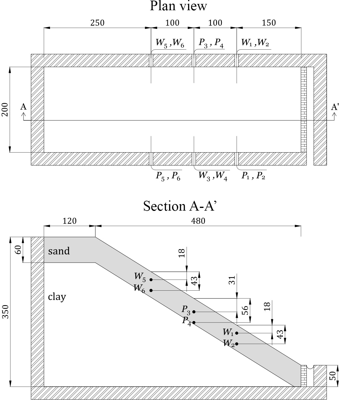
Figure 1Plan view and longitudinal cross section of the artificial hillslope, along with the position of the monitoring instruments. Tensiometers are indicated by the letter “P”, while WCR probes are denoted by “W”. All dimensions are in centimeters.
Six tensiometers and six water content reflectometer (WCR) probes are used to measure pressure head and water content in the top soil layer. All the sensors are located in an intermediate position of the hillslope, as shown in Fig. 1, which reports a plan view and longitudinal cross section along with the six positions where each tensiometer has been installed in front of the corresponding WCR. Two tipping-bucket flow gages are placed at the toe of the hillslope to measure surface runoff and subsurface outflow, while the rain is generated by a rainfall simulator that can produce relatively uniform rainfall intensities varying from 50 to 150 mm h−1 (Lora et al., 2016a).
A Campbell Scientific (CR 1000) data logger is used to collect and record all the data with a frequency of 0.5 Hz during a 12-day experiment, carried out by generating rainfall events of different duration alternated with recession periods (no rainfall, evaporation only). Before the experiment, two preliminary tests were performed to check the intensity and the uniformity of the rainfall rate. The coefficients of uniformity of the preliminary tests are equal to 72 %, for a mean rate of 58.8 mm h−1 (Lora et al., 2016a). The evaporation rate has been measured throughout the experiment by an atmometer. The average measured rate is quite small (<1 mm day−1), consistent with weather and period of the year (November 2016).
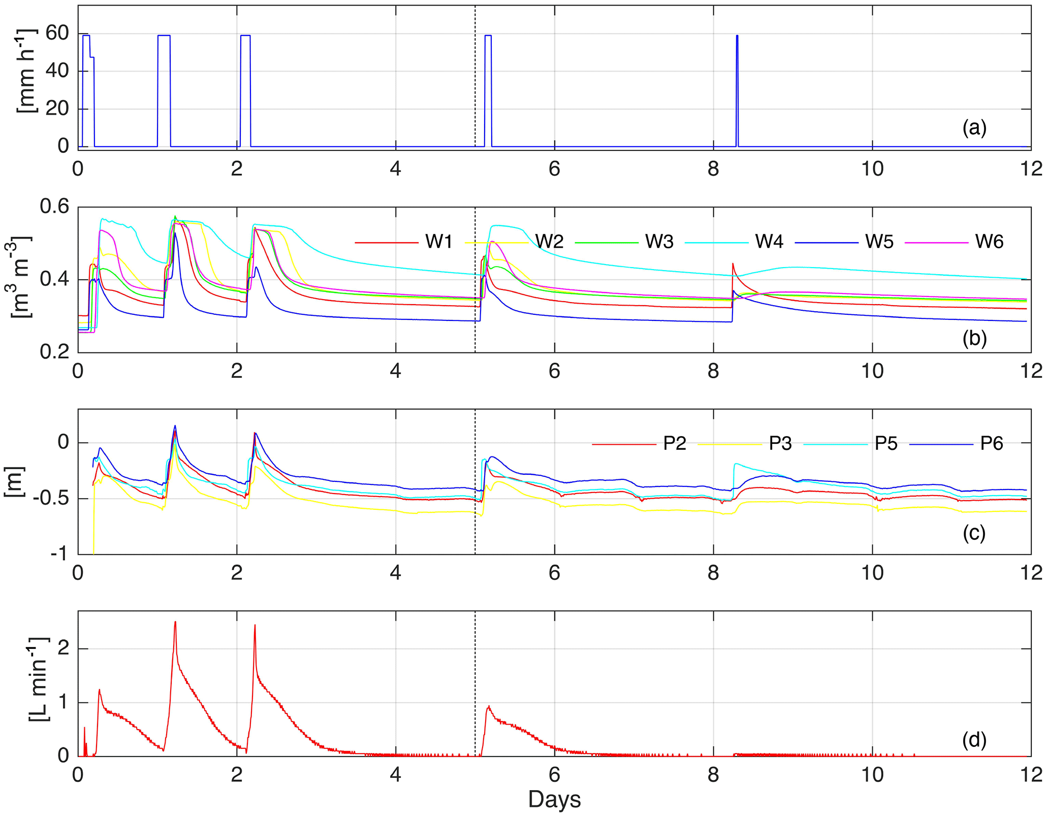
Figure 2Experimental data collected during the experiment: (a) rainfall rate; (b) water content as measured by the WCR probes; (c) pressure head as measured by the tensiometers; (d) subsurface outflow. The black vertical dashed line marks the transition between the data assimilation and the validation phases.
Figure 2 reports all the data collected during the experiment. Note that the tensiometers P1 and P4 were affected by malfunctioning; therefore, their data are not reported and were not used in the data assimilation simulations.
3.1 The CATHY model
The CATHY model (Camporese et al., 2010) is a physics-based hydrological model capable of simulating integrated subsurface, overland and channel water flow. The model combines a Richards equation solver for the three-dimensional flow in variably saturated porous media with a surface water flow module for the solution of the one-dimensional diffusion wave approximation of the de Saint-Venant equation. In this study, however, there is no surface runoff. Therefore, only subsurface flow is considered, according to the following form of the Richards equation:
In Eq. (1), is water saturation, θ and ϕ being the volumetric soil water content and porosity (∕), respectively, Ss is the specific storage coefficient (L−1), ψ is the pressure head (L), t is time (T), ∇ is the gradient operator, Ks is the saturated hydraulic conductivity tensor (L∕T), Kr is the relative hydraulic conductivity function (∕), is the vertical direction vector, z is the vertical coordinate directed upward (L), and qs represents distributed source or sink terms (L3∕L3T).
The unsaturated hydraulic properties are taken into account by means of the van Genuchten functions (e.g., Wösten and van Genuchten, 1988) Sw(ψ) and Kr(ψ):
where is the residual water saturation, with θr the residual water content, α is an empirical constant (L−1) related to the inverse of the air entry suction, and the dimensionless shape parameters n and m are linked by the expression . The model solves Eq. (1) by means of Galerkin finite elements with tetrahedral elements and linear basis functions in space and weighted finite differences for integration in time (Camporese et al., 2010).
It is worth noting that the Richards equation is strongly nonlinear, due to the retention curves (Eqs. 2 and 3). Such nonlinearities are enhanced in this study by the fact that the hillslope is characterized by dominant unsaturated conditions (Fig. 2), as opposed to many other previous applications of data assimilation with physics-based models. This makes our hillslope experiment particularly challenging and distinctive from both modeling and data assimilation perspectives.
3.2 The ensemble Kalman filter
The ensemble Kalman filter (Evensen, 2003, 2009a, b) is a sequential data assimilation scheme, in which states (and parameters) are sequentially updated based on a Monte Carlo approximation of the covariance matrices needed in the standard Kalman filter. The process is Markovian of the first order and the implementation of the EnKF does not require the linearization of the model, making it particularly suitable for handling nonlinear problems.
In this paper the EnKF is implemented according to the numerical formulation proposed by Sakov et al. (2010). Let X be an ensemble matrix of M rows and N columns, where N is the number of realizations and M is the state dimension, i.e., the number of nodes in the finite element grid, augmented by the number of parameters that are subject to update. The main idea behind this type of implementation is that the matrix X can be defined as the sum, x+A, of the ensemble average, x,
and the matrix of ensemble anomalies, A,
where 1 and I are a vector with all elements equal to one and the identity matrix, respectively. As usual, superscript T denotes matrix transposition.
Whenever observed data are available, the EnKF can compute the updated matrix Xu as the sum of the updated ensemble mean, xu, and the updated anomalies, Au:
In the following, the lack of a superscript u denotes that the matrix or vector is computed at the forecast stage, i.e., at the previous model time step.
The updated mean can be calculated as
where β is a diagonal matrix of dampening factors (Hendricks Franssen and Kinzelbach, 2008), whose elements vary from 0 to 1, and s is the scaled innovation vector
which depends on the measurement error covariance matrix, R, the difference between the measurements, D, and the ensemble mean of the simulated observations, Hx. Dampening factors help to prevent the occurrence of unstable updates and filter divergence (e.g., Evensen, 2009b) and were chosen as an alternative to covariance inflation due to ease of implementation.
The matrix G is defined as
where S is the matrix of scaled ensemble innovation anomalies
HA being the simulated measurement anomalies
and M being defined as
The updated anomalies, Au, are computed as
When updating the states only, the elements of X are the pressure heads at each node of the finite element grid, while the state augmentation technique is used when also updating the parameters. In this latter case, the desired parameters (e.g., hydraulic conductivity, parameters of the retention curves), transformed as described in Sect. 4.2, are added to X and updated based on their correlation with the system states (Erdal et al., 2015).
Table 1Perturbation parameters for the generation of the ensemble initial conditions, hydraulic conductivities and atmospheric forcing.
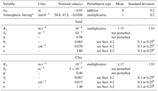
a Rainfall (positive) and evaporation (negative) rates. b σVG as described in Sect. 4.2.
4.1 CATHY setup
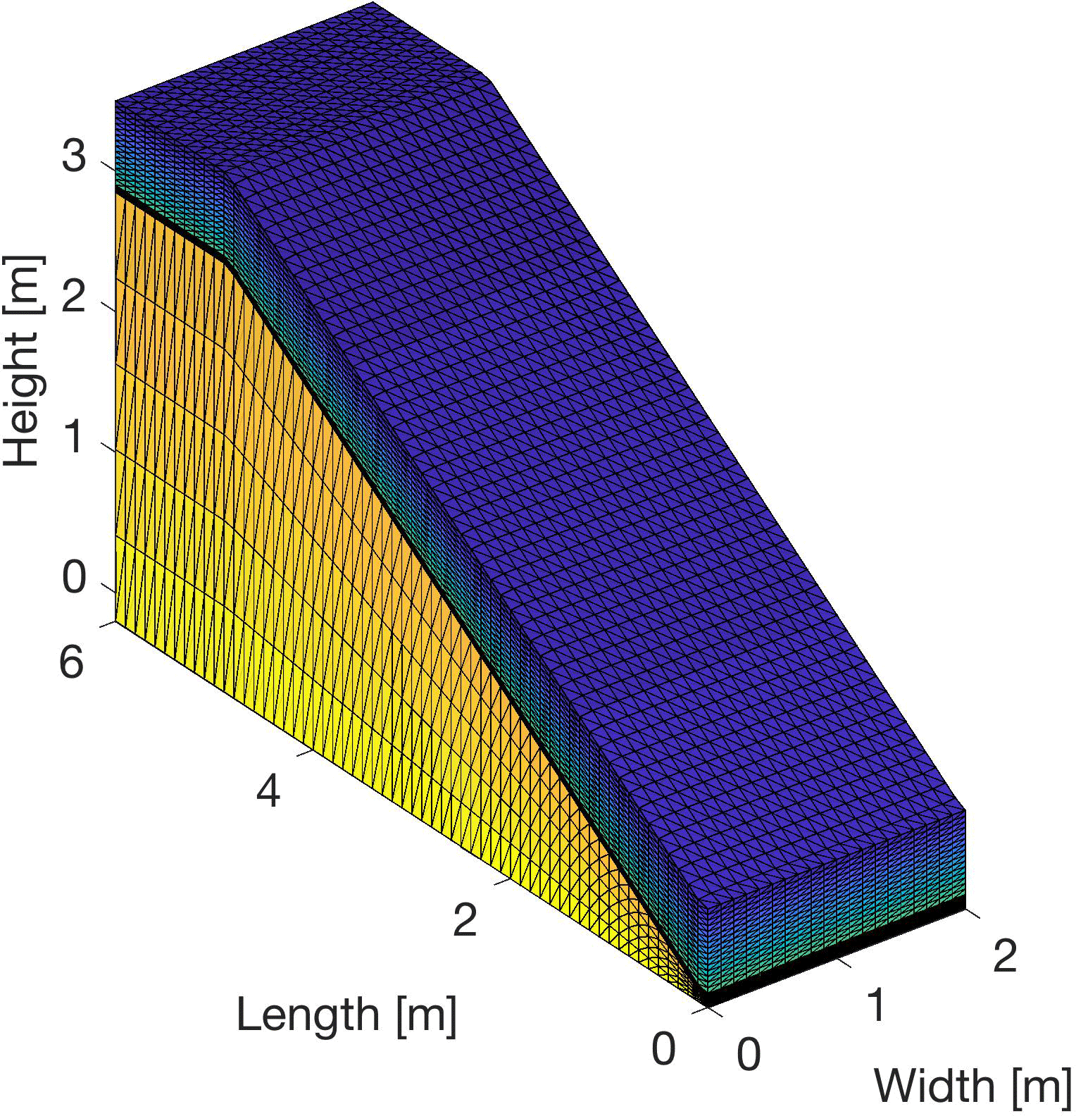
The artificial hillslope is discretized with a surface triangular grid resulting from the subdivision of square cells of 10 cm side. The triangular grid is then replicated vertically for a total of 25 layers to generate the three-dimensional tetrahedral mesh (Fig. 3). Fifteen layers are used to represent the top sand, while 10 layers discretize the clay. No flow boundary conditions are assumed at each boundary, except for the subsurface outflow section, where seepage face boundary conditions are used, and the surface, where time-variable rainfall or evaporation rates are imposed. Finally, the soil hydraulic parameters are assigned as reported in Table 1. The values of saturated hydraulic conductivity and van Genuchten retention parameters are perturbed to generate the ensemble of realizations as described in the following section, whereas soil porosities and specific storages are considered deterministic, the former being well characterized with laboratory tests and the latter having little impact on the CATHY model response in this case.
4.2 EnKF setup
In order to generate the ensemble of realizations needed for the application of the EnKF, we perturb the atmospheric forcing (i.e., rainfall and evaporation rates), soil properties and initial conditions. Table 1 reports a summary of the perturbed variables, along with their nominal mean values as well as the nature and statistics of the perturbations. The uncertainties on model parameters and boundary conditions have been assigned on the basis of previous modeling experiences and preliminary characterization of the soils in the hillslope (Camporese et al., 2009a, b; Lora et al., 2016b).
The ensemble of time-variable atmospheric forcing rates was generated with a sequence of multiplicative perturbations, qk, correlated in time as in Evensen (2003):
where the subscript k is the time index, wk is a sequence of white noise drawn from the standard normal distribution, and the coefficient γ is computed as
Δt being the assimilation interval and τ the specified time decorrelation length, here set equal to 108 000 s, i.e., 30 h.
The initial conditions consist of a uniform value of pressure head, ψ0, whose nominal ensemble mean is −0.67 m, based on the average provided by the tensiometer measurements. We opted for a uniform value of initial pressure head because, at the beginning of the experiment, the entire hillslope was in a highly unsaturated condition, as derived from the tensiometer data. This means that, even without an initially hydrostatic (i.e., equilibrium) profile, water is basically prevented from flowing in or out of the hillslope due to the very small values of relative hydraulic conductivity. This is one of the peculiarities of our test case compared to similar studies. Preliminary analyses showed that the model is not very sensitive to ψ0, because in any case the initial hydraulic conductivity is so small that the hillslope responds only when the first rainfall event occurs and starts wetting the soil. Therefore, in this study, no warm-up or spin-up was necessary. The ensemble of ψ0 values is generated by additive perturbations normally distributed with mean equal to 0 and standard deviation equal to 0.2 m.
Perturbed soil parameters, for both sand and clay, include the saturated hydraulic conductivity as well as the parameters of the van Genuchten retention curves. Table 1 reports the nominal mean values of Ks, based on soil samples analyzed in the laboratory, as well as the parameters used for generating their ensembles. The saturated hydraulic conductivities of sand and clay are perturbed independently of each other with multiplicative perturbations sampled from a lognormal distribution.
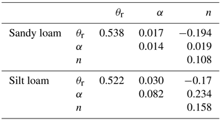
The parameters of the van Genuchten retention curves α, n, and θr are perturbed taking into account their mutual correlation according to Carsel and Parrish (1988), who described their statistics and transformed them into normally distributed variables via the Johnson system (Johnson, 1970). Three main transformation functions are available, i.e, the lognormal (LN), log-ratio (SB), and hyperbolic (SU):
where V denotes the parameter before transformation, bounded within the range [A B], and Y denotes the transformed parameter with normal distribution. In this work, the prior statistics of the van Genuchten parameters are taken from the soil types “sandy loam” and “silt loam” in Carsel and Parrish (1988), assumed as valid representations of our sand and clay, respectively. In particular, the SB transformation has been used for all the parameters, except for n of the sandy loam and α of the silt loam, for which the LN transformation has been applied. The ensemble of transformed parameters is generated by
where y is the vector containing transformed α, n, and θr, u contains the transformed variable means, T is an upper diagonal matrix, obtained from the Choleski factorization of the covariance matrix of the three parameters (see Table 2), and z is a vector of normal deviates with mean equal to 0 and standard deviation σVG. The transformed variables can be included in the matrix X when updating the parameters, and can then be back-transformed in order to obtain the updated values of the soil retention parameters.
The EnKF algorithm implemented here is actually an ensemble transform Kalman filter (Bishop et al., 2001) that does not require the perturbation of observations. On the other hand, the measurement error covariance matrix, R, must be assumed to be known a priori. In this work, R was estimated directly from the measurements, taking advantage of the high time resolution of the collected data. Pressure head and water content data were collected every 2 s and averaged every 10 min over a 40 s window to obtain the observations to assimilate. Over the same time window, the data were linearly detrended and the residuals were used to calculate the correlation coefficients between all pairs of observations. The final covariance matrices were then assembled by multiplying the correlation coefficients by the relevant standard deviations, assumed as 0.05 m and 0.025 for pressure head and water content, respectively. The subsurface outflow measurements are assumed to be independent of the pressure head and water content data, with a standard deviation equal to 8 % of the measured discharge. All measurement error standard deviations have been estimated based on the accuracy of the sensors and plausible positioning errors.
When assimilating multiple variables, proper normalization of the measurement error covariance matrices, anomalies of the simulated data, and innovation vectors were performed, using values of 0.6 m, 0.58, and m3 s−1 for pressure head, water content and subsurface outflow, respectively. The normalization ensures that in multivariate assimilation scenarios the covariance matrices in the Kalman gain are not ill-conditioned (Camporese et al., 2009b; Evensen, 2003).
Table 2Factored covariance matrices used for the perturbation of van Genuchten parameters (Carsel and Parrish, 1988).
4.3 Data assimilation scenarios
A total of 17 data assimilation scenarios have been simulated, whereby the assimilation interval, the assimilated variables, the updated variables, and the uncertainty on the van Genuchten parameters were varied. Table 3 reports a summary of the main characteristics for each scenario. Assimilated variables may include water content only or with subsurface outflow, pressure head only or with subsurface outflow, and all three variables together. With regard to the updated variables, three cases have been analyzed: update of the state variables only; update of the state variables and saturated hydraulic conductivities for both sand and clay; update of the state variables, hydraulic conductivities and van Genuchten parameters, for both sand and clay. In all the data assimilation scenarios, observations were assimilated only during the first 5 days of simulation, leaving the final 7 days as a validation period, during which the ensemble was left to evolve freely. For comparison, two open loop simulations, i.e., without data assimilation, have also been carried out (Table 3).
Table 3Overview of the open loop and data assimilation scenarios.
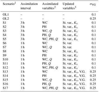
1 OL1 and OL2 indicate open loop scenarios, i.e.,
simulations without data
assimilation.
2 WC, PH, and Q denote water content, pressure
head, and subsurface
outflow, respectively.
3 St. var., Ks, and V.G. indicate state variables
(in terms of
pressure head), saturated hydraulic conductivity, and
van Genuchten parameters,
respectively.
The performance of the simulations has been evaluated by means of the root mean square error (RMSE), computed for the different variables, i.e., pressure head, water content, and subsurface outflow. The root mean square error is calculated as
where No is the number of observations available (six, four, and one for water content, pressure head, and subsurface outflow, respectively), Si,j refers to the simulated results of the ith realization of the ensemble at the location of the jth observation and Oj is the corresponding experimental value. To obtain a meaningful comparison between the errors of different variables, we also compute the time-averaged normalized root mean square error, NRMSE,
where NT is the number of time steps, k is the time index, and NF is a normalization factor equal to 0.58, 0.60 m, and m3 s−1 (i.e., 2.5 L min−1) for the water content, pressure head, and subsurface discharge, respectively. The NRMSE is computed separately for each variable and for the assimilation (NT=120) and validation (NT=167) periods, but also as a global index of performance averaged over all the variables and the two periods.
5.1 Preliminary simulations
A preliminary sensitivity analysis over a number of EnKF parameters has been performed, in order to select a final and satisfactory setup for the subsequent data assimilation scenarios. First, simulations with N equal to 32, 128 and 256 have been performed, and it has been found that an ensemble size of 128 ensures a good tradeoff between performance and computational effort. Some preliminary sensitivity analyses of the value of σVG have also been performed, resulting in values of 0.1 and 0.25 for the scenarios with and without update of van Genuchten parameters, respectively (Table 3).
Then, several dampening factor values (β in Eqs. 7 and 13) were tested, including combinations of different values for the update of system state and parameters. Based on this analysis, a value of 1 has been chosen for the update of the system state, whereas a dampening factor equal to 0.5 has been selected for the update of the soil hydraulic parameters (Ks, α, n, and θr, for both sand and clay). This choice of dampening factors is consistent with previous studies (Brandhorst et al., 2017) and prevents abrupt changes in the retention curve parameters that could lead to difficulties in model convergence and hence loss of realizations.
According to these preliminary analyses, all scenarios reported in Table 3 have been simulated with an ensemble size of 128 and dampening factors of 1 and 0.5 for system state and parameters, respectively.
5.2 Overall EnKF performance
Table 4 and Fig. 4 summarize the performance of the EnKF in all the data assimilation scenarios, expressed in terms of NRMSE for the three measured variables (water content, WC, pressure head, PH, and subsurface outflow, Q), and averaged separately over the assimilation and validation windows. A comparison between scenarios 1–5 and 8–12 in Table 4, characterized by the same assimilated and updated variables but different assimilation intervals, shows that assimilating more frequently does not always result in significant improvements of model predictions. The variable that benefits the most from more frequent updates is subsurface outflow, especially in the scenarios where Q is assimilated (e.g., compare scenarios 3–5 with 10–12).
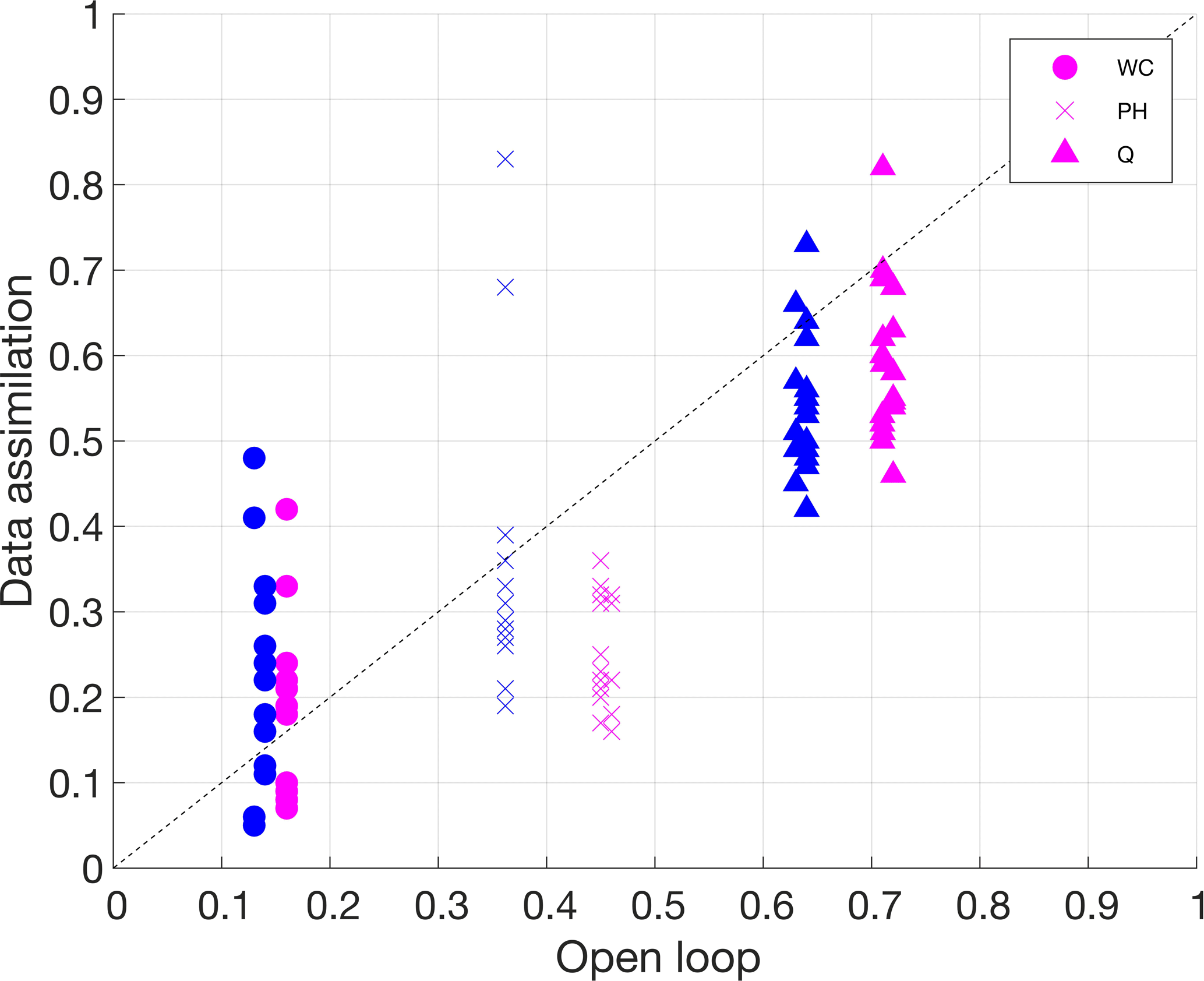
Figure 4Normalized root mean square errors for water content, pressure head, and subsurface outflow of the data assimilation scenarios versus corresponding values of the open loop. Symbols in magenta represent values calculated over the assimilation period, while symbols in blue represent values calculated over the validation period.
Figure 4 highlights that most of the data assimilation scenarios result in an improvement of model predictions for pressure head and subsurface outflow, compared to the open loop simulations (data pairs below the 45 ∘ reference line). However, in some scenarios, the filter performance in predicting the water content is actually worse than in the open loop. A close inspection of the values in Table 4 indicates that such scenarios are those where pressure head is assimilated, alone or in conjunction with water content and subsurface outflow. This is likely due to a combination of two factors: (i) only four out of six tensiometers are available for assimilation, compared to the six WCR probes available for water content, and (ii) the pressure head measurements are characterized by relatively poor quality. This can be appreciated from the pressure head data shown in Fig. 2, where diurnal disturbances caused by temperature fluctuations (Warrick et al., 1998) are apparent.
Table 4Normalized root mean square errors (NRMSEs) for the 17 data assimilation scenarios under analysis and two open loop (OL) simulations. The table reports the NRMSE for three variables, water content, pressure head and outflow discharge, for both the assimilation and the validation periods. The last three columns report the mean values calculated over the three variables (WC, PH and Q) and the global average between assimilation and validation. Bold values indicate exceedance of the corresponding open loop errors.
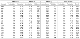
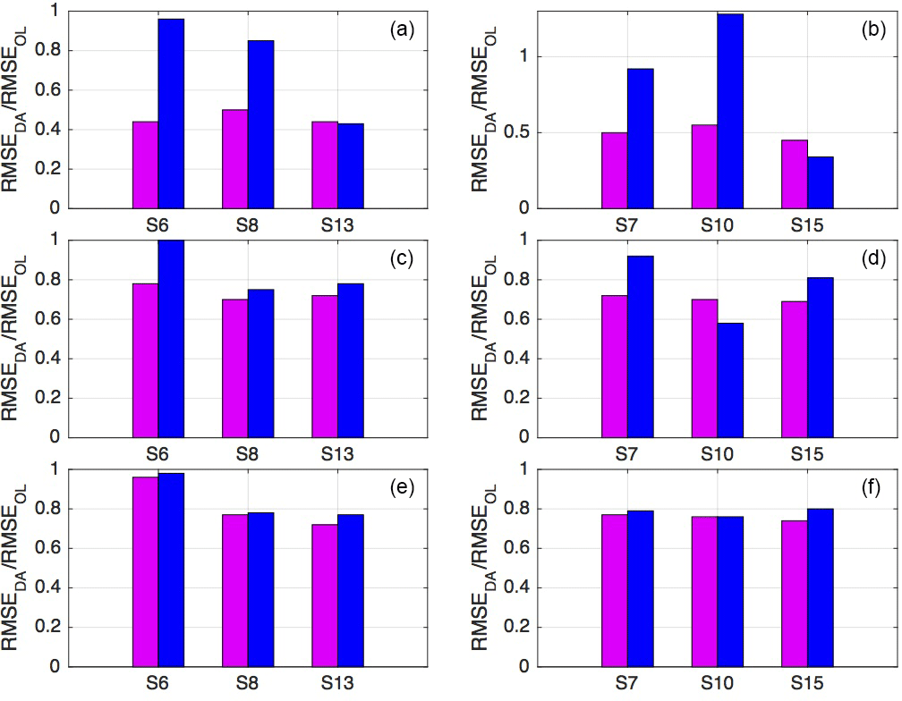
Figure 5Ratios between RMSEs in scenarios S6, S8, and S13 (a, c, e), S7, S10, and S15 (b, d, f), and the corresponding open loop values, for water content, WC (a, b), pressure head, PH (c, d), and subsurface outflow, Q (e, f). The magenta bars refer to the data assimilation period, and the blue ones to the validation period.
5.3 Parameter estimation capabilities
To assess the capabilities and benefits of parameter estimation with the EnKF, it is useful to compare scenarios with the same assimilated variables but different updated variables. Figure 5a, c, and e show the ratios between RMSE in data assimilation scenarios S6, S8, and S13 and the corresponding open loop values for water content, pressure head, and subsurface outflow, respectively. In these three scenarios, water content alone is assimilated, but the updated variables are system state only in S6, system state and saturated hydraulic conductivity in S8, and system state, the Ks and van Genuchten parameters α, n, and θr in S13. Figure 5a highlights that progressively updating more parameters brings significant improvements in water content prediction over the validation period, with reductions of the NRMSE with respect to the open loop of almost 20 % when updating Ks only and 60 % when also updating the retention curve parameters. Moreover, updating parameters improves significantly pressure head predictions in validation and subsurface outflow in both assimilation and validation, as shown in Fig. 5c and e.
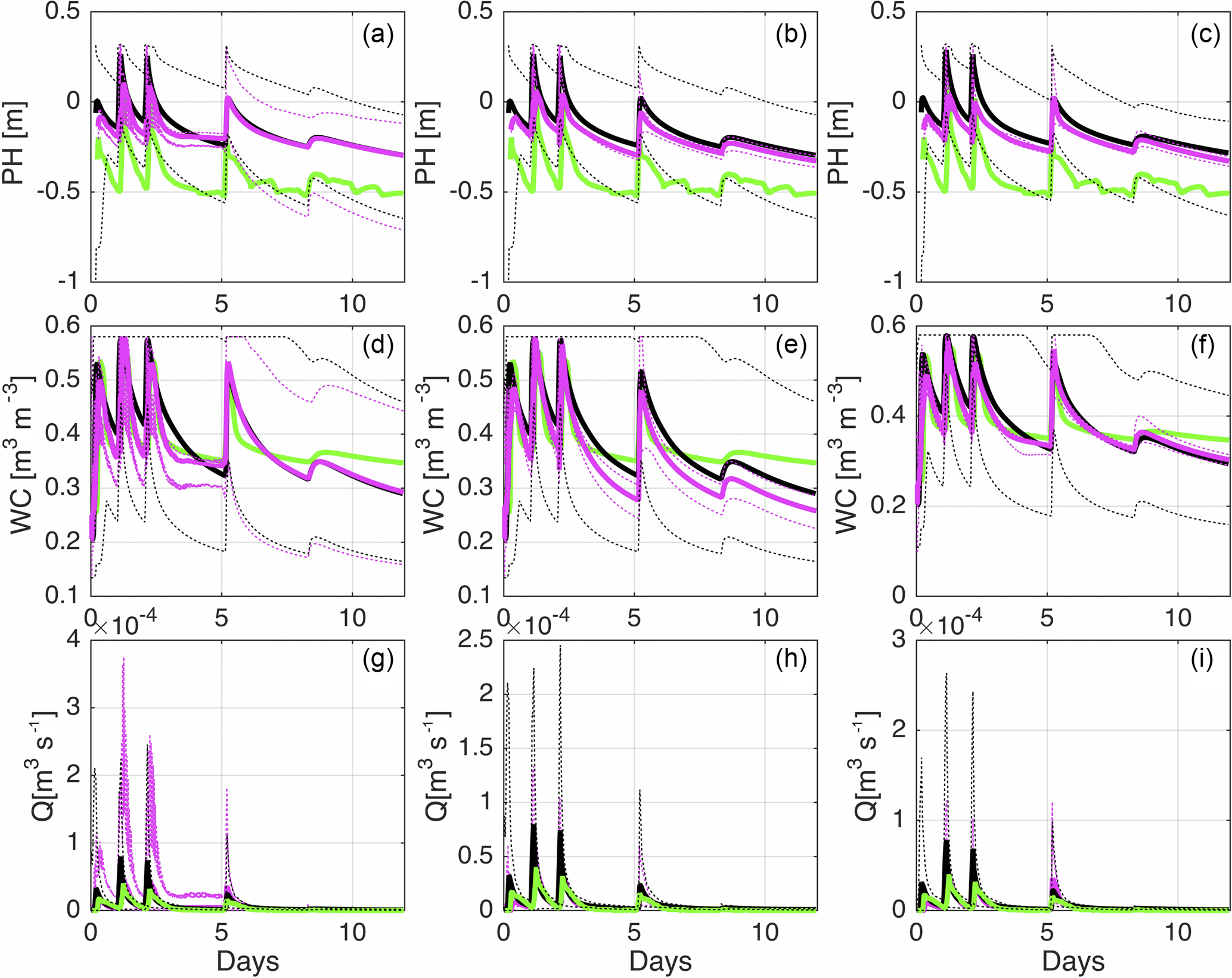
Figure 6Plots of the pressure head in P2 (a, b, c), water content in W6 (d, e, f), and outflow discharge (g, h, i) for scenarios S6 (a, d, g), S8 (b, e, h), and S13 (c, f, i). Solid green lines represent experimental data, while solid black and magenta lines indicate the ensemble mean of the open loop and data assimilation scenarios, respectively. The simulated 90 % confidence bands are also reported (dashed black and magenta lines). The locations of the tensiometer P2 and water content probe W6 are shown in Fig. 1.
The effect of parameter updating on model predictions for scenarios S6, S8, and S13 can be visualized in Fig. 6, which shows ensemble means and 90 % confidence bands of simulated water content, pressure head, and subsurface outflow in comparison with the experimental data and the corresponding open loop values. In scenario S6, without parameter update, model predictions during the validation tend to converge again to the open loop simulations in terms of both mean and uncertainty (Fig. 6a, d, g). Updating the parameters (scenarios S8 and S13) results in decreased uncertainty during validation (Fig. 6b, c, e, f, h, i), due to the reduced variability of saturated hydraulic conductivity and van Genuchten parameters. Note also that the update of Ks is particularly beneficial to pressure head (panel a versus b and c, where it can be seen that, in the validation phase, the ensemble mean with data assimilation departs the open loop and gets closer to the measurements) and subsurface outflow (panel g versus h and i), whereas updating α, n, and θr improved significantly the water content (panel e versus f).
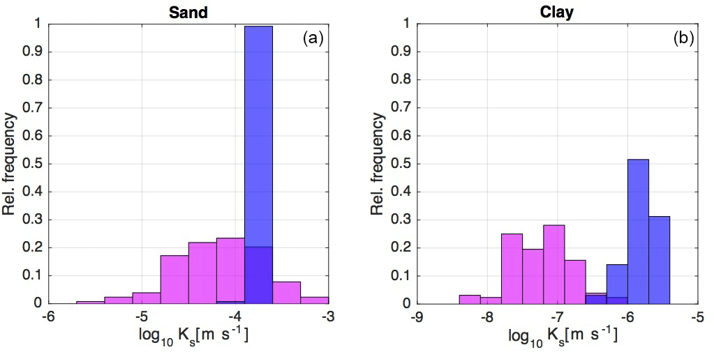
Figure 7Relative frequency distributions of the saturated hydraulic conductivity, Ks, of sand and clay in scenario S10. Graphs in magenta denote the prior Ks distributions, while the blue ones indicate the posterior distributions, i.e., at the end of the assimilation period.
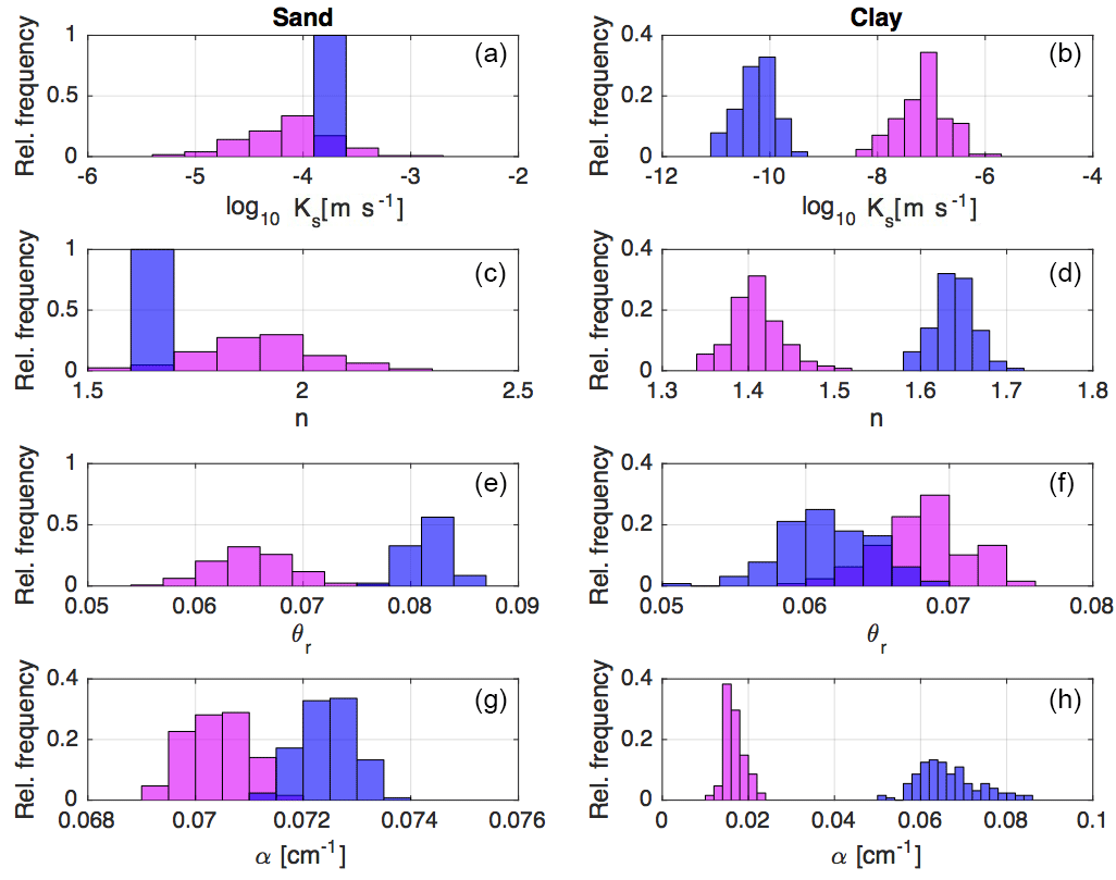
Figure 8Relative frequency distributions of the saturated hydraulic conductivity, Ks, and van Genucthen parameters of sand and clay in scenario S15. Graphs in magenta denote prior distributions, while the blue ones indicate posterior distributions, i.e., at the end of the assimilation period.
5.4 Tradeoffs in multi-source data assimilation
We now focus our attention on the scenarios where multi-source data are assimilated. The right panels in Fig. 5 show the ratios between RMSE in data assimilation scenarios S7, S10, and S15 and the corresponding open loop values for water content, pressure head, and subsurface outflow. Whereas in scenarios S6, S8, and S13 (see panels (a), (c) and (e) in Fig. 5) water content alone was assimilated, in scenarios S7, S10, and S15 (see panels (b), (d) and (f) in Fig. 5) water content and subsurface outflow were jointly assimilated. The updated variables are system state only in S7, system state and saturated hydraulic conductivity in S10, and system state plus Ks and van Genuchten parameters α, n, and θr in S15. As previously noted for the scenarios with assimilation of water content alone, the effect of parameter updating is significant mainly in the validation phase. However, one can now observe an increase in validation RMSE of water content when also updating Ks, with a value that exceeds the one of the corresponding open loop. At the same time, there is a decrease in pressure head RMSE of more than 40 % with respect to the open loop, indicating that the update of Ks is beneficial to pressure head, but not to water content. Including the update of van Genuchten parameters, in scenario S15, has an opposite effect: model predictions of water content in validation improve dramatically (RMSE of almost 60 % less than in the open loop), whereas pressure head predictions worsen slightly and align with RMSE values of scenario S13. This indicates that the update of the van Genuchten parameters is more important for predictions of water content than pressure head, which represents an interesting example of the kinds of tradeoffs associated with multi-source data assimilation and parameter updating in integrated hydrological models.
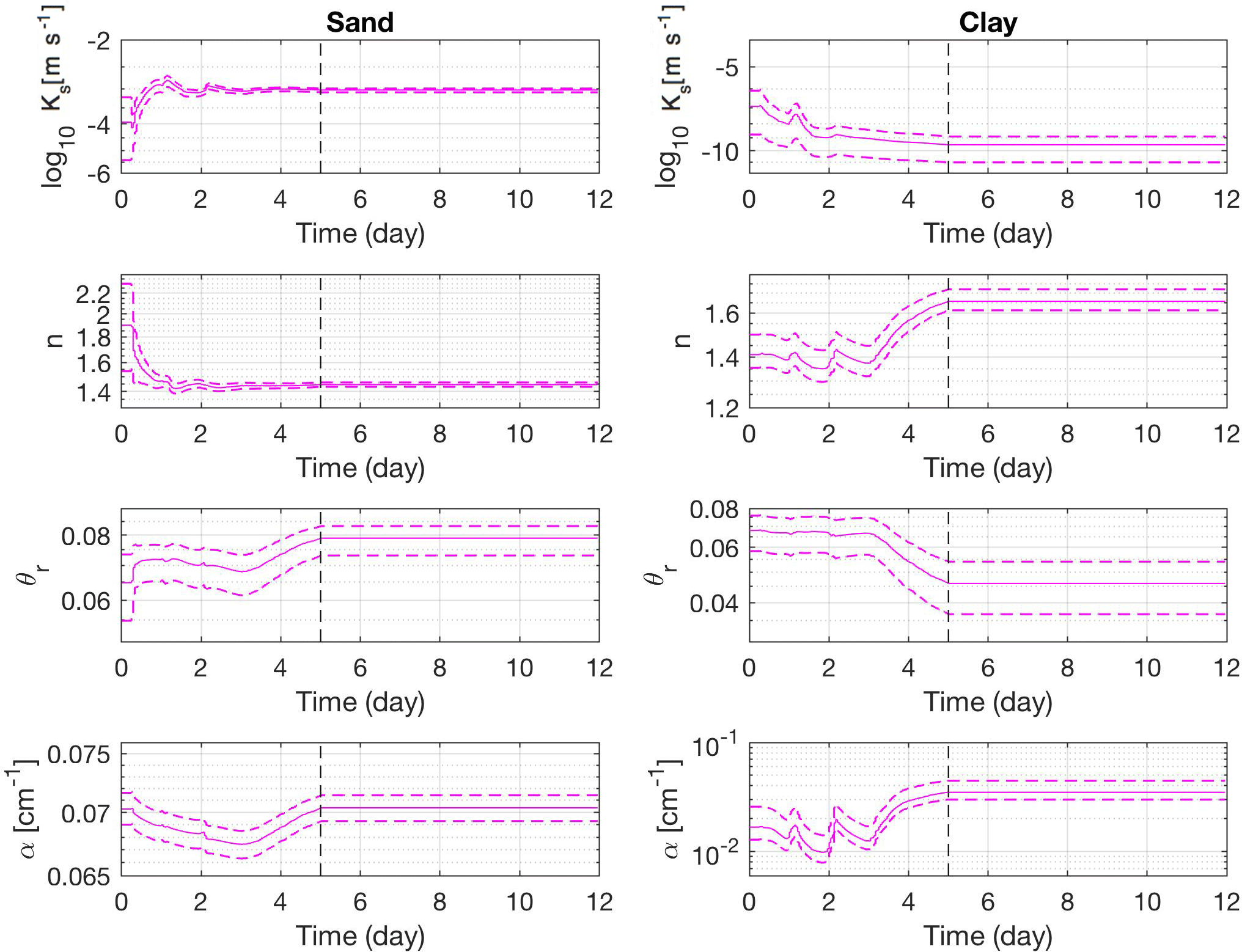
Figure 9Time evolution of the saturated hydraulic conductivity and van Genuchten parameters (mean values, solid line, together with minimum and maximum values, in dashed lines, to indicate the ensemble spread) for the two types of soil, sand and clay, in scenario S17.
Further insights into the differences between scenarios S10 and S15 can be gained from Figs. 7 and 8, which report the prior and posterior (i.e., at the end of the assimilation period) distributions of soil parameters. Fig. 7 reports the results for scenario S10, where Ks only was updated, and shows that the sand Ks is clearly identifiable, whereas the clay Ks is not, with a large residual uncertainty and a mean value that is not consistent with the actual soil type in the hillslope. As no data are available in the clay layer, the large residual variability should be expected, but the bias in the mean value is probably caused by spurious correlations and, perhaps, also by the low sensitivity of the assimilated variables to the clay permeability. This is likely the reason for the poor model prediction of water content.
Figure 8 shows the prior and posterior distributions of Ks, α, n, and θr in S15. Again, for the sand, the saturated hydraulic conductivity can be clearly identified, as well as the exponent n of the van Genuchten retention function, while parameters θr and α are more difficult to estimate. As for the clay, posterior uncertainty is large for all the parameters and the mean value of Ks shows again a bias with respect to the prior value, although in this case the final value is more consistent with the actual soil type and this could explain why the water content model predictions improve significantly compared to scenario S10. This can also be explained by the fact that all the sensors are located in the sand layer, while no experimental data from the clay layer are assimilated.
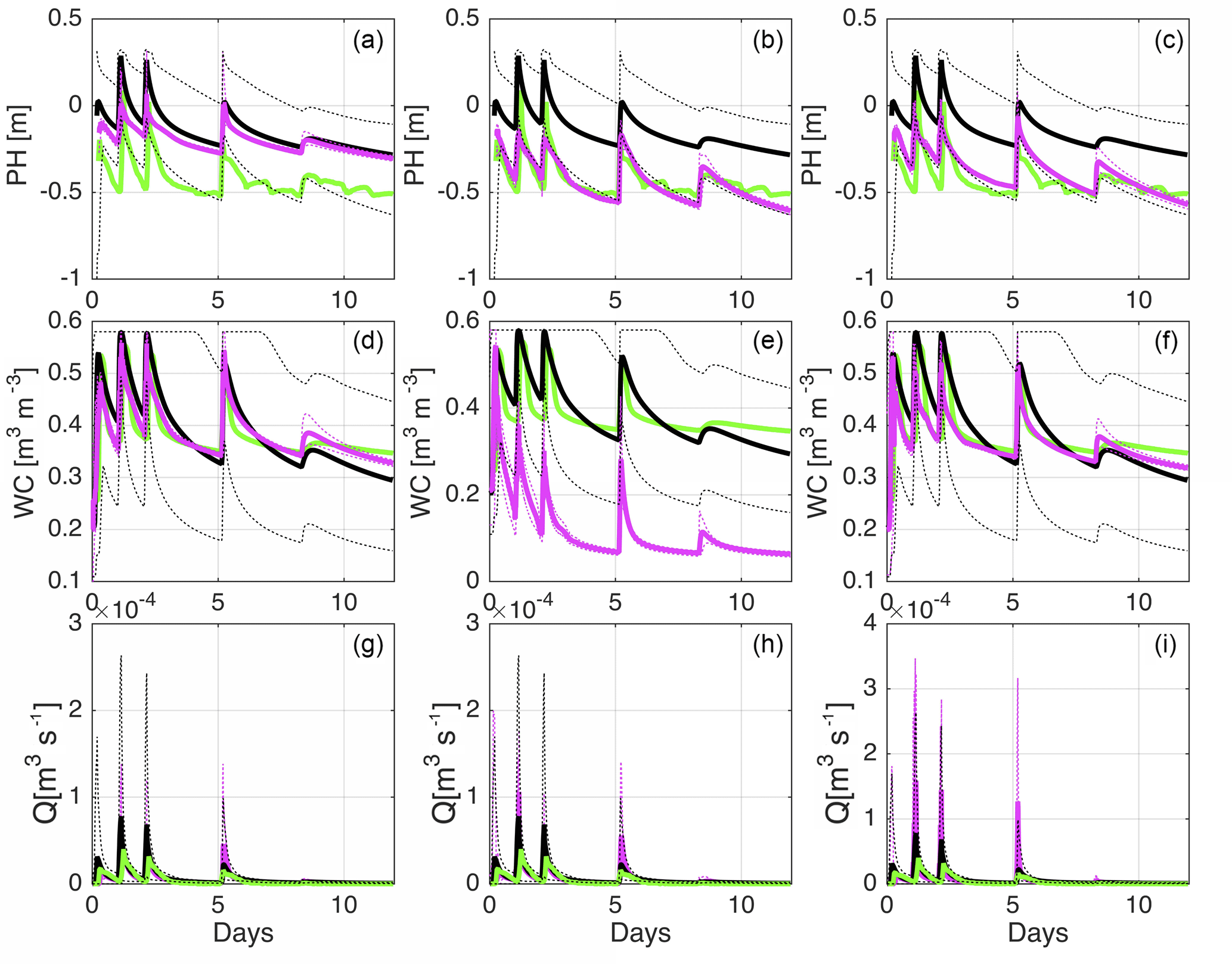
Figure 10Plots of the pressure head in P2, (a, b, c), water content in W6, (d, e, f) and outflow discharge (g, h, i) for scenarios S15 (a, d, g), S16 (b, e, h), and S17 (c, f, i). Solid green lines represent experimental data, while solid black and magenta lines indicate the ensemble mean of the open loop and data assimilation scenarios, respectively. The simulated 90 % confidence bands are also reported (dashed black and magenta lines). The locations of the tensiometer P2 and water content probe W6 are shown in Fig. 1.
An additional perspective on parameter estimation is given by Fig. 9, which shows the time evolution of ensemble mean and spread of the saturated hydraulic conductivity and van Genuchten parameters for both sand and clay in scenario S17 (one of the scenarios reported in Fig. 10). The convergence toward stable values in the data assimilation phase is only achieved for the parameters Ks and n of the sand layer, while the dispersion remains generally higher for θr (to which the model is typically not very sensitive) and α, as well as for all the parameters of the clay layer.
In summary, the results of parameter updating for the clay show that data would be needed in all the soil layers. However, when dealing with large heterogeneous structures, it is very expensive to have every soil zone properly probed, which is why it is important to assess whether multivariate data assimilation approaches are capable of compensating for the lack of distributed observations with alternative sources of information. Here, an integrated measurement such as the subsurface outflow does not seem to be sufficient to compensate for this lack of representativeness.
Finally, we analyze the tradeoffs in system state predictions associated with multi-source data assimilation for scenarios S15, S16, and S17. Figure 10 shows pressure head in P2, water content in W6, and subsurface outflow as simulated in the data assimilation and open loop scenarios, in terms of ensemble mean and 90 % confidence bands, compared to the measurements. In scenario S15 (Fig. 10a, d, g), where water content and subsurface discharge were assimilated, model results are very good for these variables but not so for pressure head (see also NRMSE values in Table 4). On the other hand, in scenario S16, where pressure head and subsurface outflow were assimilated, pressure head and discharge are well simulated, but not water content (Fig. 10b, e, h, and Table 4). Finally, in scenario S17, where all the available data were assimilated, the model predicts well both pressure head and water content, but at the cost of a slightly degraded prediction of subsurface outflow compared to scenarios S15 and S16 (Fig. 10c, f, i, and Table 4).
Similar issues were reported by Zhang et al. (2016), who found that the joint assimilation of soil moisture and groundwater head does not improve model predictions, unless update localization is used. In their study, this was likely caused by unrealistic cross-variable correlations due to limited ensemble sizes, whereas in our case it might be that the relatively poor quality of pressure head measurements, compared to water content observations, and the lack of observations in the clay layer do not allow us to obtain accurate estimates of the van Genuchten parameters.
In this study, a Richards equation-based hydrological model, CATHY, has been used with the ensemble Kalman filter to assimilate pressure head, water content, and subsurface outflow data in a real-world test case, represented by an experimental artificial hillslope. A total of 17 data assimilation simulations have been presented and described to provide a comprehensive overview of possible scenarios. Univariate scenarios with the assimilation of water content or pressure head alone were compared to multivariate cases where water content and pressure head were combined with outflow discharge or where water content, pressure head and outflow discharge were jointly assimilated. Regarding the updating strategies, single (state variable) and joint (state variables plus saturated hydraulic conductivity with and without van Genuchten parameters) updating scenarios were considered.
Overall, the capabilities of the ensemble Kalman filter to jointly correct the system states and soil parameters in physically based hydrological models were confirmed, even in a real-world test case such as the one presented here, characterized by dominant unsaturated dynamics and hence strong nonlinearities. Updating of the saturated hydraulic conductivity brought significant improvements in the prediction of pressure head and subsurface outflow, while updating the van Genuchten parameters proved to be highly beneficial to the prediction of the water content dynamics. On the other hand, multivariate data assimilation may lead to significant tradeoffs. For instance, the assimilation of soil moisture in addition to pressure head and subsurface outflow improved water content, but slightly degraded the prediction of the outflow discharge. Moreover, our results suggest that high-quality and representative data are essential for a proper and effective use of data assimilation in physically based hydrological models, as shown by the relatively poor performance of the EnKF in scenarios when pressure head was assimilated, due to temperature disturbances of the data, and by biased estimates of clay parameters, due to the lack of data in this soil layer.
In future studies, more representative data, including observations in the clay, will be assimilated, and the possibility of applying bias-aware filters will be considered to compensate for the effect of temperature in the tensiometric data.
All the data are available from the corresponding author upon request.
AB and EB carried out the experiment. AB conducted the numerical simulations. AB and MC wrote the manuscript. MC supervised the research. All the authors reviewed the manuscript.
The authors declare that they have no conflict of interest.
We gratefully acknowledge the financial support of the University of Padua,
through grant CPDA148790. We thank the editor and three anonymous reviewers
for their detailed and very helpful comments.
Edited by: Harrie-Jan Hendricks Franssen
Reviewed by: three
anonymous referees
Baatz, D., Kurtz, W., Franssen, H. H., Vereecken, H., and Kollet, S.: Catchment tomography – An approach for spatial parameter estimation, Adv. Water Resour., 107, 147–159, https://doi.org/10.1016/j.advwatres.2017.06.006, 2017. a
Bailey, R. and Baù, D.: Ensemble smoother assimilation of hydraulic head and return flow data to estimate hydraulic conductivity distribution, Water Resour. Res., 46, w12543, https://doi.org/10.1029/2010WR009147, 2010. a
Bauser, H. H., Jaumann, S., Berg, D., and Roth, K.: EnKF with closed-eye period – towards a consistent aggregation of information in soil hydrology, Hydrol. Earth Syst. Sci., 20, 4999–5014, 10.5194/hess-20-4999-2016, 2016. a
Bishop, C. H., Etherton, B. J., and Majumdar, S. J.: Adaptive Sampling with the Ensemble Transform Kalman Filter. Part I: Theoretical Aspects, Mon. Weather Rev., 129, 420–436, https://doi.org/10.1175/1520-0493(2001)129<0420:ASWTET>2.0.CO;2, 2001. a
Brandhorst, N., Erdal, D., and Neuweiler, I.: Soil moisture prediction with the ensemble Kalman filter: Handling uncertainty of soil hydraulic parameters, Adv. Water Resour., 110, 360–370, https://doi.org/10.1016/j.advwatres.2017.10.022, 2017. a, b
Cammalleri, C. and Ciraolo, G.: State and parameter update in a coupled energy/hydrologic balance model using ensemble Kalman filtering, J. Hydrol., 416–417, 171–181, https://doi.org/10.1016/j.jhydrol.2011.11.049, 2012. a
Camporese, M., Paniconi, C., Putti, M., and Salandin, P.: Ensemble Kalman filter data assimilation for a process-based catchment scale model of surface and subsurface flow, Water Resour. Res., 45, w10421, https://doi.org/10.1029/2008WR007031, 2009a. a, b
Camporese, M., Paniconi, C., Putti, M., and Salandin, P.: Comparison of Data Assimilation Techniques for a Coupled Model of Surface and Subsurface Flow, Vadose Zone J., 8, 837–845, https://doi.org/10.2136/vzj2009.0018, 2009b. a, b, c
Camporese, M., Paniconi, C., Putti, M., and Orlandini, S.: Surface-subsurface flow modeling with path-based runoff routing, boundary condition-based coupling, and assimilation of multisource observation data, Water Resour. Res., 46, w02512, https://doi.org/10.1029/2008WR007536, 2010. a, b, c
Carsel, R. F. and Parrish, R. S.: Developing joint probability distributions of soil water retention characteristics, Water Resour. Res., 24, 755–769, https://doi.org/10.1029/WR024i005p00755, 1988. a, b, c
Chen, Y. and Zhang, D.: Data assimilation for transient flow in geologic formations via ensemble Kalman filter, Adv. Water Resour., 29, 1107–1122, https://doi.org/10.1016/j.advwatres.2005.09.007, 2006. a
Clark, M. P., Rupp, D. E., Woods, R. A., Zheng, X., Ibbitt, R. P., Slater, A. G., Schmidt, J., and Uddstrom, M. J.: Hydrological data assimilation with the ensemble Kalman filter: Use of streamflow observations to update states in a distributed hydrological model, Adv. Water Resour., 31, 1309–1324, https://doi.org/10.1016/j.advwatres.2008.06.005, 2008. a
Crow, W. T. and Wood, E. F.: The assimilation of remotely sensed soil brightness temperature imagery into a land surface model using Ensemble Kalman filtering: a case study based on ESTAR measurements during SGP97, Adv. Water Resour., 26, 137–149, https://doi.org/10.1016/S0309-1708(02)00088-X, 2003. a
De Lannoy, G. J., Houser, P. R., Pauwels, V., and Verhoest, N. E.: State and bias estimation for soil moisture profiles by an ensemble Kalman filter: Effect of assimilation depth and frequency, Water Resour. Res., 43, 6, https://doi.org/10.1029/2006WR005100, 2007. a, b
Erdal, D., Neuweiler, I., and Wollschläger, U.: Using a bias aware EnKF to account for unresolved structure in an unsaturated zone model, Water Resour. Res., 50, 132–147, https://doi.org/10.1002/2012WR013443, 2014. a
Erdal, D., Rahman, M., and Neuweiler, I.: The importance of state transformations when using the ensemble Kalman filter for unsaturated flow modeling: Dealing with strong nonlinearities, Adv. Water Resour., 86, 354–365, https://doi.org/10.1016/j.advwatres.2015.09.008, 2015. a
Evensen, G.: The Ensemble Kalman Filter: theoretical formulation and practical implementation, Ocean Dynam., 53, 343–367, 2003. a, b, c, d
Evensen, G.: Data Assimilation: The Ensemble Kalman Filter, Springer-Verlag, Berlin, Germany, 2009a. a
Evensen, G.: The ensemble Kalman filter for combined state and parameter estimation, vol. 29, IEEE Control Systems, 83–104, 2009b. a, b, c
Flores, A. N., Bras, R. L., and Entekhabi, D.: Hydrologic data assimilation with a hillslope-scale-resolving model and L band radar observations: Synthetic experiments with the ensemble Kalman filter, Water Resour. Res., 48, W08509, https://doi.org/10.1029/2011WR011500, 2012. a
Francois, C., Quesney, A., and Ottlé, C.: Sequential Assimilation of ERS-1 SAR Data into a Coupled Land Surface–Hydrological Model Using an Extended Kalman Filter, J. Hydrometeorol., 4, 473–487, 2003. a
Hain, C. R., Crow, W. T., Anderson, M. C., and Mecikalski, J. R.: An ensemble Kalman filter dual assimilation of thermal infrared and microwave satellite observations of soil moisture into the Noah land surface model, Water Resour. Res., 48, 11, https://doi.org/10.1029/2011WR011268, 2012. a
Han, X. and Li, X.: An evaluation of the nonlinear/non-Gaussian filters for the sequential data assimilation, Remote Sens. Environ., 112, 1434–1449, 2008. a
Hendricks Franssen, H. J. and Kinzelbach, W.: Real-time groundwater flow modeling with the Ensemble Kalman Filter: Joint estimation of states and parameters and the filter inbreeding problem, Water Resour. Res., 44, w09408, https://doi.org/10.1029/2007WR006505, 2008. a, b
Johnson, S. K.: Distributions in Statistics: Continuous Unvariate Distributions-1, Houghton Mifflin, 1970. a
Kollet, S., Sulis, M., Maxwell, R. M., Paniconi, C., Putti, M., Bertoldi, G., Coon, E. T., Cordano, E., Endrizzi, S., Kikinzon, E., Mouche, E., Mügler, C., Park, Y.-J., Refsgaard, J. C., Stisen, S., and Sudicky, E.: The integrated hydrologic model intercomparison project, IH-MIP2: A second set of benchmark results to diagnose integrated hydrology and feedbacks, Water Resour. Res., 53, 867–890, https://doi.org/10.1002/2016WR019191, 2017. a
Kurtz, W., He, G., Kollet, S. J., Maxwell, R. M., Vereecken, H., and Hendricks Franssen, H.-J.: TerrSysMP–PDAF (version 1.0): a modular high-performance data assimilation framework for an integrated land surface–subsurface model, Geosci. Model Dev., 9, 1341–1360, 10.5194/gmd-9-1341-2016, 2016. a
Li, L., Zhou, H., Gómez-Hernández, J. J., and Franssen, H.-J. H.: Jointly mapping hydraulic conductivity and porosity by assimilating concentration data via ensemble Kalman filter, J. Hydrol., 428–429, 152–169, 2012. a
Lora, M., Camporese, M., and Salandin, P.: Design and performance of a nozzle-type rainfall simulator for landslide triggering experiments, CATENA, 140, 77–89, https://doi.org/10.1016/j.catena.2016.01.018, 2016a. a, b, c
Lora, M., Camporese, M., Troch, P. A., and Salandin, P.: Rainfall-triggered shallow landslides: infiltration dynamics in a physical hillslope model, Hydrol. Process., 30, 3239–3251, https://doi.org/10.1002/hyp.10829, 2016b. a
Maxwell, R. M., Putti, M., Meyerhoff, S., Delfs, J.-O., Ferguson, I. M., Ivanov, V., Kim, J., Kolditz, O., Kollet, S. J., Kumar, M., Lopez, S., Niu, J., Paniconi, C., Park, Y.-J., Phanikumar, M. S., Shen, C., Sudicky, E. A., and Sulis, M.: Surface-subsurface model intercomparison: A first set of benchmark results to diagnose integrated hydrology and feedbacks, Water Resour. Res., 50, 1531–1549, https://doi.org/10.1002/2013WR013725, 2014. a
Monsivais-Huertero, A., Graham, W. D., Judge, J., and Agrawal, D.: Effect of simultaneous state-parameter estimation and forcing uncertainties on root-zone soil moisture for dynamic vegetation using EnKF, Adv. Water Resour., 33, 468–484, https://doi.org/10.1016/j.advwatres.2010.01.011, 2010. a
Montzka, C., Pauwels, V. R. N., Franssen, H.-J. H., Han, X., and Vereecken, H.: Multivariate and Multiscale Data Assimilation in Terrestrial Systems: A Review, Sensors, 12, 16291–16333, https://doi.org/10.3390/s121216291, 2012. a
Moradkhani, H.: Hydrologic remote sensing and land surface data assimilation, Sensors, 8, 2986–3004, 2008., a
Moradkhani, H., Hsu, K.-L., Gupta, H., and Sorooshian, S.: Uncertainty assessment of hydrologic model states and parameters: Sequential data assimilation using the particle filter, Water Resour. Res., 41, 5, https://doi.org/10.1029/2004WR003604, 2005. a
Pan, M. and Wood, E. F.: Data Assimilation for Estimating the Terrestrial Water Budget Using a Constrained Ensemble Kalman Filter, J. Hydrometeorol., 7, 534–547, https://doi.org/10.1175/JHM495.1, 2006. a
Pasetto, D., Camporese, M., and Putti, M.: Ensemble Kalman filter versus particle filter for a physically-based coupled surface–subsurface model, Adv. Water Resour., 47, 1–13, 2012. a
Pasetto, D., Niu, G.-Y., Pangle, L., Paniconi, C., Putti, M., and Troch, P. A.: Impact of sensor failure on the observability of flow dynamics at the Biosphere 2 LEO hillslopes, Adv. Water Resour., 86, 327–339, https://doi.org/10.1016/j.advwatres.2015.04.014, 2015. a
Rasmussen, J., Madsen, H., Jensen, K. H., and Refsgaard, J. C.: Data assimilation in integrated hydrological modeling using ensemble Kalman filtering: evaluating the effect of ensemble size and localization on filter performance, Hydrol. Earth Syst. Sci., 19, 2999–3013, 10.5194/hess-19-2999-2015, 2015. a
Rasmussen, J., Madsen, H., Jensen, K. H., and Refsgaard, J. C.: Data assimilation in integrated hydrological modelling in the presence of observation bias, Hydrol. Earth Syst. Sci., 20, 2103–2118, 10.5194/hess-20-2103-2016, 2016. a
Reichle, R. H., McLaughlin, D. B., and Entekhabi, D.: Hydrologic data assimilation with the ensemble Kalman filter, Mon. Weather Rev., 130, 103–114, 2002a. a
Reichle, R. H., Walker, J. P., Koster, R. D., and Houser, P. R.: Extended versus ensemble Kalman filtering for land data assimilation, J. Hydrometeorol., 3, 728–740, 2002b. a
Ridler, M.-E., Madsen, H., Stisen, S., Bircher, S., and Fensholt, R.: Assimilation of SMOS-derived soil moisture in a fully integrated hydrological and soil-vegetation-atmosphere transfer model in Western Denmark, Water Resour. Res., 50, 8962–8981, https://doi.org/10.1002/2014WR015392, 2014. a
Sakov, P., Evensen, G., and Bertino, L.: Asynchronous data assimilation with the EnKF, Tellus A, 62, 24–29, https://doi.org/10.1111/j.1600-0870.2009.00417.x, 2010. a
Schenato, L., Palmieri, L., Camporese, M., Bersan, S., Cola, S., Pasuto, A., Galtarossa, A., Salandin, P., and Simonini, P.: Distributed optical fibre sensing for early detection of shallow landslides triggering, Sci. Rep., 7, 14686, https://doi.org/10.1038/s41598-017-12610-1, 2017. a
Shi, Y., Davis, K. J., Zhang, F., Duffy, C. J., and Yu, X.: Parameter estimation of a physically-based land surface hydrologic model using an ensemble Kalman filter: A multivariate real-data experiment, Adv. Water Resour., 83, 421–427, https://doi.org/10.1016/j.advwatres.2015.06.009, 2015. a
Tang, Q., Kurtz, W., Schilling, O., Brunner, P., Vereecken, H., and Franssen, H.-J. H.: The influence of riverbed heterogeneity patterns on river-aquifer exchange fluxes under different connection regimes, J. Hydrol., 554, 383–396, https://doi.org/10.1016/j.jhydrol.2017.09.031, 2017. a
Troch, P. A., Paniconi, C., and McLaughlin, D.: Catchment-scale hydrological modeling and data assimilation, Adv. Water Resour., 26, 131–135, https://doi.org/10.1016/S0309-1708(02)00087-8, 2003. a
Visser, A., Stuurman, R., and Bierkens, M. F.: Real-time forecasting of water table depth and soil moisture profiles, Adv. Water Resour., 29, 692–706, 2006. a
Vrugt, J. A., Gupta, H. V., Nualláin, B., and Bouten, W.: Real-Time Data Assimilation for Operational Ensemble Streamflow Forecasting, J. Hydrometeorol., 7, 548–565, https://doi.org/10.1175/JHM504.1, 2006. a
Warrick, A. W., Wierenga, P. J., Young, M. H., and Musil, S. A.: Diurnal fluctuations of tensiometric readings due to surface temperature changes, Water Resour. Res., 34, 2863–2869, https://doi.org/10.1029/98WR02095, 1998. a
Weerts, A. H. and El Serafy, G. Y.: Particle filtering and ensemble Kalman filtering for state updating with hydrological conceptual rainfall-runoff models, Water Resour. Res., 42, W09403, https://doi.org/10.1029/2005WR004093, 2006. a
Wösten, J. H. M. and van Genuchten, M. T.: Using Texture and Other Soil Properties to Predict the Unsaturated Soil Hydraulic Functions, Soil Sci. Soc. Am. J., 52, 1762–1770, 1988. a
Xie, X. and Zhang, D.: Data assimilation for distributed hydrological catchment modeling via ensemble Kalman filter, Adv. Water Resour., 33, 678–690, https://doi.org/10.1016/j.advwatres.2010.03.012, 2010. a
Zhang, D., Madsen, H., Ridler, M. E., Refsgaard, J. C., and Jensen, K. H.: Impact of uncertainty description on assimilating hydraulic head in the MIKE SHE distributed hydrological model, Adv. Water Resour., 86, 400–413, https://doi.org/10.1016/j.advwatres.2015.07.018, 2015. a
Zhang, D., Madsen, H., Ridler, M. E., Kidmose, J., Jensen, K. H., and Refsgaard, J. C.: Multivariate hydrological data assimilation of soil moisture and groundwater head, Hydrol. Earth Syst. Sci., 20, 4341–4357, 10.5194/hess-20-4341-2016, 2016. a, b, c
Zhang, H., Kurtz, W., Kollet, S., Vereecken, H., and Franssen, H.-J. H.: Comparison of different assimilation methodologies of groundwater levels to improve predictions of root zone soil moisture with an integrated terrestrial system model, Adv. Water Resour., 111, 224–238, https://doi.org/10.1016/j.advwatres.2017.11.003, 2018. a, b
Zovi, F., Camporese, M., Franssen, H.-J. H., Huisman, J. A., and Salandin, P.: Identification of high-permeability subsurface structures with multiple point geostatistics and normal score ensemble Kalman filter, J. Hydrol., 548, 208–224, https://doi.org/10.1016/j.jhydrol.2017.02.056, 2017. a