the Creative Commons Attribution 4.0 License.
the Creative Commons Attribution 4.0 License.
 | 20 Aug 2018
Surface water monitoring in small water bodies: potential and limits of multi-sensor Landsat time series
Gilles Belaud
Sylvain Massuel
Mark Mulligan
Patrick Le Goulven
Roger Calvez
Hydrometric monitoring of small water bodies (1–10 ha) remains rare, due to their limited size and large numbers, preventing accurate assessments of their agricultural potential or their cumulative influence in watershed hydrology. Landsat imagery has shown its potential to support mapping of small water bodies, but the influence of their limited surface areas, vegetation growth, and rapid flood dynamics on long-term surface water monitoring remains unquantified. A semi-automated method is developed here to assess and optimize the potential of multi-sensor Landsat time series to monitor surface water extent and mean water availability in these small water bodies. Extensive hydrometric field data (1999–2014) for seven small reservoirs within the Merguellil catchment in central Tunisia and SPOT imagery are used to calibrate the method and explore its limits. The Modified Normalised Difference Water Index (MNDWI) is shown out of six commonly used water detection indices to provide high overall accuracy and threshold stability during high and low floods, leading to a mean surface area error below 15 %. Applied to 546 Landsat 5, 7, and 8 images over 1999–2014, the method reproduces surface water extent variations across small lakes with high skill (R2=0.9) and a mean root mean square error (RMSE) of 9300 m2. Comparison with published global water datasets reveals a mean RMSE of 21 800 m2 (+134 %) on the same lakes and highlights the value of a tailored MNDWI approach to improve hydrological monitoring in small lakes and reduce omission errors of flooded vegetation. The rise in relative errors due to the larger proportion and influence of mixed pixels restricts surface water monitoring below 3 ha with Landsat (Normalised RMSE = 27 %). Interferences from clouds and scan line corrector failure on ETM+ after 2003 also decrease the number of operational images by 51 %, reducing performance on lakes with rapid flood declines. Combining Landsat observations with 10 m pansharpened Sentinel-2 imagery further reduces RMSE to 5200 m2, displaying the increased opportunities for surface water monitoring in small water bodies after 2015.
- Article
(30898 KB) - Full-text XML
- BibTeX
- EndNote


1.1 Monitoring water resources in small reservoirs
Support from governmental and international projects combined with farmer initiatives have led to significant development of small reservoirs (<1 Mm3) across the globe, including India (Bouma et al., 2011; Massuel et al., 2014; Venot and Krishnan, 2011), Brazil (Burte et al., 2005), and parts of northern and sub-Saharan Africa (Nyssen et al., 2010; Sawunyama et al., 2006; Talineau et al., 1994). These have been built to reduce sediment transfer and silting of downstream dams, as well as to harvest scarce and unreliable water resources for local users (Habi and Morsli, 2011; Wisser et al., 2010).
Despite their growing importance worldwide, small reservoirs are rarely monitored in situ, except for research purposes (Albergel and Rejeb, 1997), due to their quantity, size, and geographical dispersion. Instrumenting and maintaining a hydrometric observation network require significant time, equipment, and transport costs (Liebe et al., 2005) which are not compatible with the localized and modest importance in the water budget of small reservoirs. As a result, little information is available on their water availability and their cumulative influence (Ogilvie et al., 2016b).
Water availability in small reservoirs is constrained by design capacities but determined by site-specific hydrological dynamics regulated by both natural (climate, topography, geology, geomorphology, pedology) and human factors (maintenance, leaks, withdrawals, releases). Studies based on hydrological measurements and geochemical analyses have identified the water balance of small reservoirs (Gay, 2004; Grunberger et al., 2004; Lacombe, 2007; Li and Gowing, 2005; Nyssen et al., 2010) but highlighted multiple modelling uncertainties due to evaporation, groundwater flows, high spatial rainfall variability, and human management (Grunberger et al., 2004; Kingumbi et al., 2007; Lacombe, 2007; Leduc et al., 2007; Li and Gowing, 2005). Rainfall–runoff modelling of gauged small reservoirs in Tunisia notably failed to exceed R2=0.5 (Lacombe, 2007) and difficulties are greater in ungauged catchments (Cudennec et al., 2005).
1.2 Remote sensing in hydrology
Images from a variety of active and passive sensors have been used successfully in hydrology to inventory and to assess flooded areas and river stage levels and widths, as well as to investigate hydrological processes and water balance issues. Low spatial resolution sensors such as MODIS (Moderate Resolution Imaging Spectroradiometer, 250 m) and AVHRR (Advanced Very High Resolution Radiometer, 1.1 km), providing daily coverage of the globe, notably facilitated the assessment and monitoring of large wetlands (Guo et al., 2017), including the Niger Inner Delta (Bergé-Nguyen and Crétaux, 2015; Mahé et al., 2011; Ogilvie et al., 2015; Seiler et al., 2009), the Okavango Delta (Gumbricht et al., 2004; Wolski and Murray-Hudson, 2008), the Tana Delta (Leauthaud et al., 2013), or the Mekong Delta (Kuenzer et al., 2015; Sakamoto et al., 2007), large rivers such as the Amazon (Alsdorf et al., 2007; Martinez and Le Toan, 2007), and large lakes notably in eastern Africa (Ouma and Tateishi, 2006; Swenson and Wahr, 2009) and China (Ma et al., 2007; Qi et al., 2009). These sensors have also been used for global assessments (Klein et al., 2015; Papa et al., 2010; Prigent et al., 2007), but their low spatial resolutions remain inadequate for small reservoirs, as a single MODIS pixel corresponds to an area of 6.25 ha.
High spatial resolution imagery such as SPOT (Satellite Pour l'Observation de la Terre), Quickbird, and Ikonos captures images under 5 m resolution, but their reduced spatial coverage (10–20 km wide for the highest resolution) makes them less suitable for medium-sized catchments and their costs are prohibitive for operational long-term monitoring. Recent sensors such as Sentinel-2 capture 10 m images of the entire globe every 5 days, providing enhanced opportunities, but hydrological investigations which require historical perspectives will continue to rely on previous sensors. Landsat, which has provided free multispectral images since the 1970s at medium geometric resolution (30 m since Landsat 4 in 1982) every 16 days (since Landsat 7 in 1999, as previous sensors present multiple gaps), therefore continues to provide the most potential to detect and monitor small water bodies.
Satellite altimetry originally developed to monitor the ocean's surface has increasingly been exploited and adapted since the 1990s to monitor height variations of continental surface waters (Crétaux et al., 2016). Used across rivers and large lakes, recent works have sought to transpose these to smaller water bodies (from 50 ha), but highlight several limitations relating essentially to the poor density of altimetry tracks, the long along-track path lengths, and low revisit times (Avisse et al., 2017; Baup et al., 2014). Altimeters aboard Topex, Envisat, Jason-1, and Jason-2 have temporal resolutions ranging from 10 to 35 days and high vertical accuracy; however, their narrow swaths and long along-track path lengths (1 km) restrict their application essentially to large lakes (>100 km2, Avisse et al., 2017). Other altimeters have improved spatial resolution and cover more of the globe but at the expense of low revisit times (368 days for Cryostat-2), removing any monitoring possibilities. The Dahiti altimetry database (Schwatke et al., 2015), employed by Busker et al. (2018), combines the tracks of numerous altimeters to optimize the sites covered, temporal resolution, and length of observations. These provide data for 168 sites in Africa (none however in Tunisia) and lakes must have a minimum 300 m diameter (circa 7 ha). The Sentinel-3a and 3b constellations provide major improvements in their along-track resolution (300 m), making them potentially suitable for lakes around 4 ha, but inter-tracks of 52 km mean many lakes are not covered by their trajectories (Crétaux et al., 2016). Furthermore, radar altimetry provides an estimate of the altitude of the water surface, based on the two-way travel time of the radar pulse and the known altitude of the satellite, but assessing absolute volumes requires site-specific data such as stage height or topographic data (Baup et al., 2014). Avisse et al. (2017) showed that DEM data taken before lakes were built or when they were empty could be used, but on larger lakes (59 to 379 ha) with 30 m data.
1.3 Landsat imagery to map and monitor small water bodies
Local studies on small lakes from 1 to 25 ha in western Africa (Annor et al., 2009; Gardelle et al., 2010; Jones et al., 2017; Liebe et al., 2005; Soti et al., 2010), in southern Africa (Sawunyama et al., 2006), in southern India (Mialhe et al., 2008), and in South America (Rodrigues et al., 2011) specifically investigated the potential of remote sensing methods to assess surface areas of small reservoirs. Field validation confirmed the potential of remote sensing (RS) methods as a cost-effective technique to identify water bodies, but revealed problems of variable accuracy (Annor et al., 2009; Ran and Lu, 2012; Solander et al., 2016) on small lakes (under 100 ha). These studies provided a snapshot of floods in reservoirs at a given time (Liebe et al., 2005), or of seasonality (Annor et al., 2009; Jones et al., 2017), but did not explore their dynamics over time.
Smaller water bodies have also been included in worldwide inventories, done with Landsat imagery (Feng et al., 2016; Verpoorter et al., 2014; Yamazaki et al., 2015). Landsat was recently used to undertake long-term monitoring of surface water bodies at global (Pekel et al., 2016) and regional scales (Avisse et al., 2017; Mueller et al., 2016; Tulbure et al., 2016). The remarkable study by Pekel et al. (2016) exploited 1 petabyte of Landsat archive imagery to study surface water dynamics in 30 m pixels globally over 1984–2015. Small water bodies were included, but Yamazaki and Trigg (2016) warn of limitations in Pekel et al. (2016) as “resolution issues prevent analysis of small water bodies”. Similarly, Mueller et al. (2016), focussing on Australian water bodies, recognized the difficulties in the “presence of water and vegetation within the pixel” and that their “product may not be fit for […] small farm dams”. In their own inventory of water bodies, Yamazaki et al. (2015) had also noted the omission errors on water bodies below 100 ha. These errors on small lakes are influenced by the insufficient spatial resolution, but essentially also by the increased presence of flooded vegetation and shallow waters which affect the reflectance signal (Annor et al., 2009; Mueller et al., 2016; Sawunyama et al., 2006; Yamazaki et al., 2015). These studies recognize the difficulties of using Landsat imagery, but adequate ground truth data remain sparse and extensive field validation has not quantified the limits of these approaches on the smallest lakes. The feasibility of Landsat to monitor surface water dynamics and provide long-term water availability assessments in small water bodies remains therefore to be quantified (Baup et al., 2014; Pekel et al., 2016). Validation depends on higher-resolution imagery or other published water maps which suffer from similar classification inaccuracies (Yamazaki et al., 2015), non-negligible on these small water bodies. Pekel et al. (2016) for example in their validation used sample pixels of seasonal water bodies within 1∘ tiles, but these did not specifically account for small water bodies as shown in this paper.
Furthermore, hydrological monitoring of small water bodies imposes specific constraints on temporal resolution, due to the limited flood amplitude and the rapid flood declines, and “with the 16 day repeat cycle of Landsat […] floods may be missed” (Yamazaki and Trigg, 2016). Clouds and shadows in optical imagery as well as the scan line corrector failure (after 31 May 2003 on the Landsat 7 ETM+ sensor) are known to have a detrimental influence in global water datasets (Mueller et al., 2016; Pekel et al., 2016). These have a proportionally larger influence on small water bodies where gap-fill methods are not suited to localized rapid changes in land cover (Zeng et al., 2013; Zhu and Woodcock, 2014). The influence of Landsat's limited temporal resolution and these interferences on representing flood dynamics in small lakes remains however unknown.
1.4 Improving surface water monitoring in small reservoirs
The objective of this research was to assess and optimize the ability of Landsat to provide sufficient, accurate observations of long-term surface water dynamics in the smallest water bodies (1–10 ha). Exceptional long-term hydrological time series of seven small reservoirs over up to 15 years are used here to develop and validate a semi-automated method using Landsat imagery, capable of reproducing surface water dynamics and long-term water availability in small water bodies.
(McFeeters, 1996)(Xu, 2006)(Lacaux et al., 2007)(Gao, 1996)(Lacaux et al., 2007)(Rouse et al., 1973)(Feyisa et al., 2014)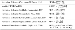
Numerous spectral water indices and classification methods exist, but these are often tested and developed empirically on larger water bodies (Feyisa et al., 2014) and their suitability in different settings must be investigated (Palmer et al., 2015). Suitable automation of water detection over several reservoirs and over several images also imposes specific constraints on the methodology, in terms of detection accuracy, threshold stability, cloud presence, and computer processing when manipulating satellite imagery (Mialhe et al., 2008; Ogilvie et al., 2015; Pekel et al., 2016). Widely used water detection indices were compared to assess their suitability for monitoring floods on small reservoirs. The interferences from clouds, shadows, and scan-line corrector failure were investigated and reduced here by defining optimal filter thresholds based on long-term field data. Results were compared with analysis performed using available global water datasets (Pekel et al., 2016) to quantify accuracy issues and argue for the benefits of specific approaches for small water bodies. Finally, the benefits provided by Sentinel-2 imagery for surface water monitoring since 2015 were quantified.
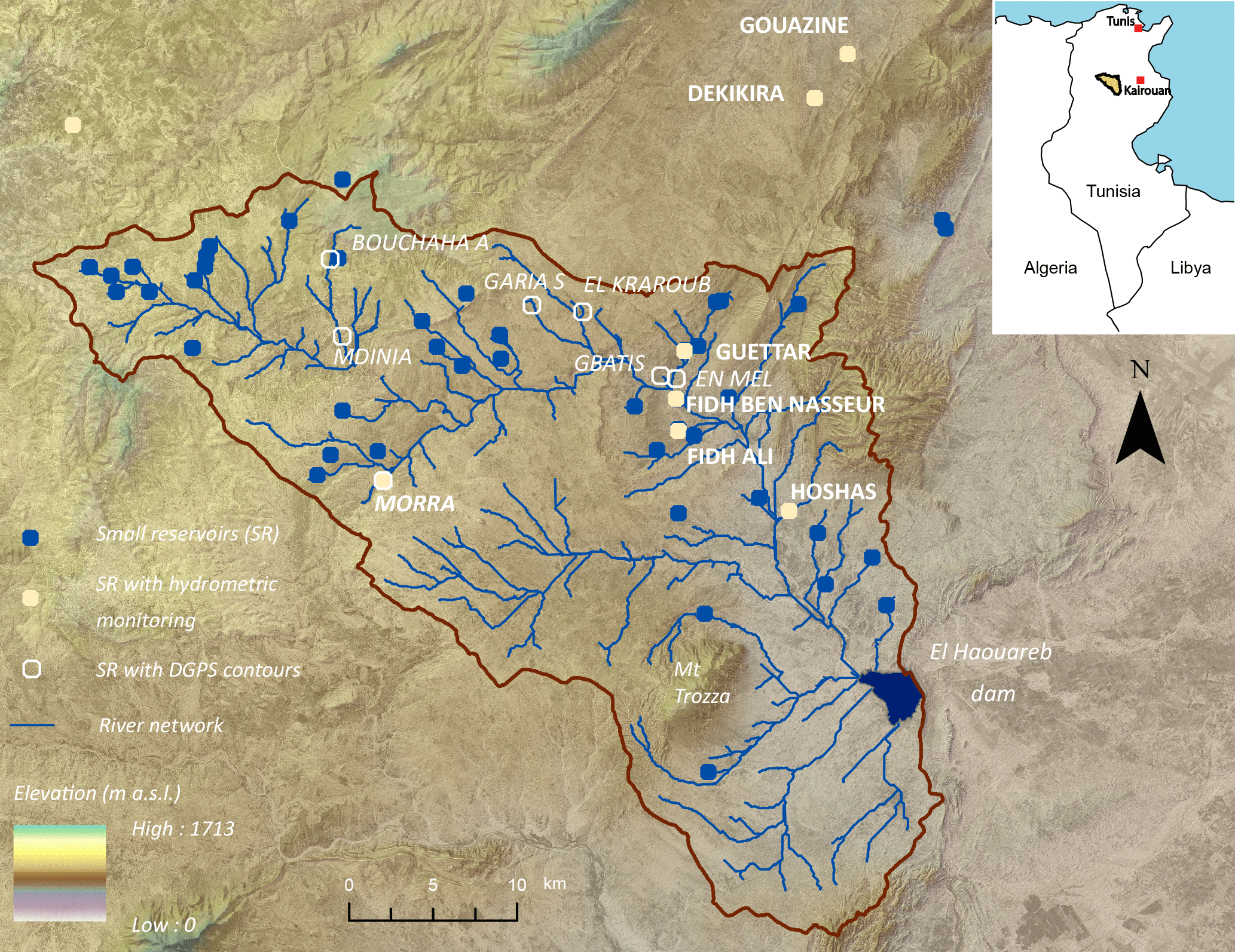
2.1 Small reservoirs in the Merguellil upper catchment
The case study area is the Merguellil upper catchment located in central semi-arid Tunisia (Fig. 1). A total of 58 small reservoirs have been built across this 1180 km2 catchment since the 1960s, as a result of international projects and an ambitious nationwide water and soil conservation strategy. These were inventoried through the combination and cross-referencing of records from local authorities, literature (CNEA, 2006; Kingumbi, 2006; Lacombe, 2007), satellite imagery, and field visits (Ogilvie et al., 2016a).
Initial design capacities of small reservoirs in the catchment range between 17 000 and 1 590 000 m3, though the median size only reaches 66 000 m3. Peak flooded surface areas vary between 0.5 and 18 ha. Lakes flood as a result of intense localized rainfall events (Ogilvie et al., 2016b), during autumn and spring mostly. High annual and interannual variability in rainfall (329 mm year−1 ±131 mm) combined with significant heterogeneity in the infiltration, evaporation rates, and occasional withdrawals lead to large disparities in the frequency and duration of floods in small lakes (Lacombe, 2007; Ogilvie, 2015).
Table 2Landsat 8 MNDWI flooded surface area assessments compared to field measurements for seven lakes on the calibration and validation images .
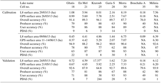
*46 % of clouds and 50 % of shadows were detected over this lake on this L8 image.
Due to the importance of the downstream irrigated Kairouan plain for national agricultural production, the catchment has been the focus of numerous research projects to understand the changes and influences exerted by evolving climatic and human dynamics (dam and small reservoir construction, irrigation withdrawals, etc.). Small reservoirs in the Merguellil upper catchment and along the Tunisian NE–SW mountain range (“Dorsale”) consequently benefited from extensive hydrological monitoring thanks to ongoing research collaboration with the local authorities (Albergel and Rejeb, 1997).
2.2 Field hydrometric monitoring
Seven reservoirs helped calibrate and validate the spectral water indices. Lakes were chosen amongst those identified as flooded on a classified 10 m SPOT image in March 2013, and flooded surface areas were measured with real-time kinematic (RTK) GPS, to reduce uncertainties from stage–height rating curves. Nineteen GPS contours were acquired, providing a range of flooded surface areas from 0.2 to 7.8 ha (Table 2) to test the performance of indices.
Seven small reservoirs with extensive field data were then used to test the performance of the method over time, i.e. identify how spatial and temporal resolution affected monitoring of surface water extent dynamics and water availability. Lakes were selected based on the length and quality of their hydrometric time series (Fig. 2) and include a range of altitudes (Fig. 1), capacities (Table 3), and associated flood dynamics (amplitude and duration). With the exception of Lake Morra, these seven lakes were not used in the calibration of the indices, giving further weight and confidence to the validation of their thresholds.
Reservoir levels were monitored with automatic stage pressure transducers and daily readings by local observers on limnimetric stage ladders were used to cross-check and fill gaps in automatic readings. Following the decline in the number and quality of observations exacerbated by the Tunisian revolution, complementary instrumentation was implemented on three small reservoirs, Guettar, Morra, and Hoshas, as part of this research. Transducer uncertainties are minimal, with a 0.2 cm resolution and theoretical ±0.25 % precision.
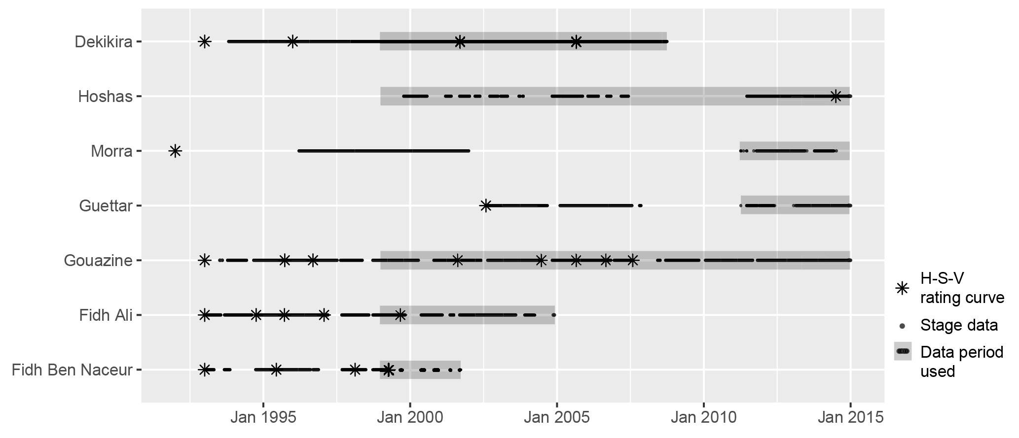
Figure 2Availability of stage data and rating curves over 1992–2014 for the seven lakes monitored.
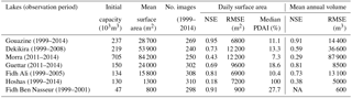
Table 3Landsat RS performance on daily surface areas and mean annual volumes.
2.2.1 Lake hypsometric relationships
Stage values were converted to surface areas and water volumes using rating curves available for each lake, indicated in Fig. 2. These were acquired and updated to account for silting as part of regular surveys started in the late 1990s (Albergel and Rejeb, 1997). A complementary survey was undertaken on Hoshas in 2014 with a RTK GPS and interpolated based on Delaunay triangular interpolation networks (TINs), well suited to bathymetric applications. Considering the logistical difficulties in updating rating curves (cost, access to lake, presence of water and dense vegetation on the lake bed), complementary field data were used to assess uncertainties associated with the obsolescence of the rating curves. Figure 3 shows that mean surface area error from the rating curve against two additional GPS contours acquired on Guettar and five on Morra reaches 1450 and 9000 m2 respectively. In relative terms these remain low (11 %–12 %) in both cases despite rating curves not being updated for 12 and 22 years respectively. Errors rise for smaller surface areas (Fig. 3) and in catchments with higher silting rates such as Fidh Ali (Collinet and Zante, 2005; Hentati et al., 2010). Comparing surface areas calculated with the Gouazine 2001 and 2007 rating curves provided an estimate of the error generated from a 6-year old rating curve and accordingly an indication of errors on surface areas calculated until 2014. Mean RMSE reaches 2300 m2 for surface areas under 10 ha but rises to 5200 m2 for surface areas below 1 ha. Similarly, on Fidh Ali after 4 years, mean RMSE reaches 4600 m2 on flooded areas under 4 ha but rises for both small (6700 m2 for S<1 ha) and larger (5600 m2 for S>3 ha) surface areas.
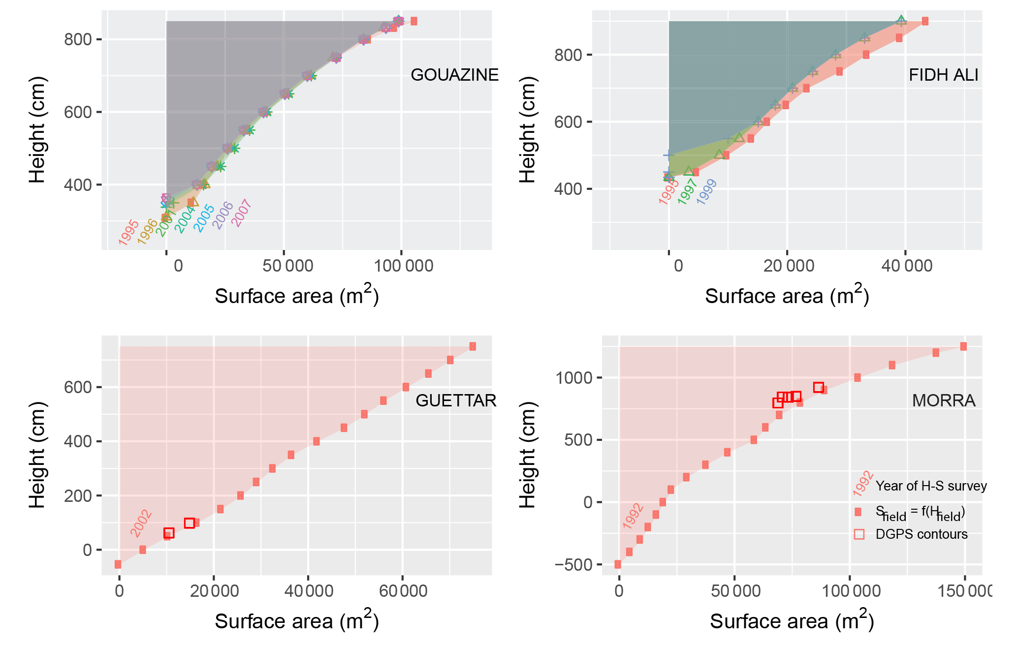
Analysis in the region (Albergel et al., 2003; Lacombe, 2007) of 70 height (H) – surface (S) – volume (V) rating curves expressed as power relations (e.g. ) showed that the shift in the parameters (B, β) over time due to silting could be modelled through linear regression. Parameters evolve to reflect the decreasingly concave nature of the lake banks. In ungauged reservoirs, such regional power relations are required, but relative errors can exceed 50 % (Liebe et al., 2005; Ogilvie et al., 2016a; Sawunyama et al., 2006). In gauged reservoirs, these estimates also lead to rising uncertainties over time, as silting is not a linear, incremental process. Sediment transport is heterogeneous and occurs through sudden, discrete events, difficult to model in these small catchments (Hentati et al., 2010). On Morra, estimating silt deposit after 22 years leads to a RMSE of over 60 000 m2 when compared to the GPS contours, confirming the difficulty of updating the initial rating curve. The influences of the rating curves on the assessment of the performance of Landsat monitoring are further discussed in the results.
2.3 Landsat preprocessing
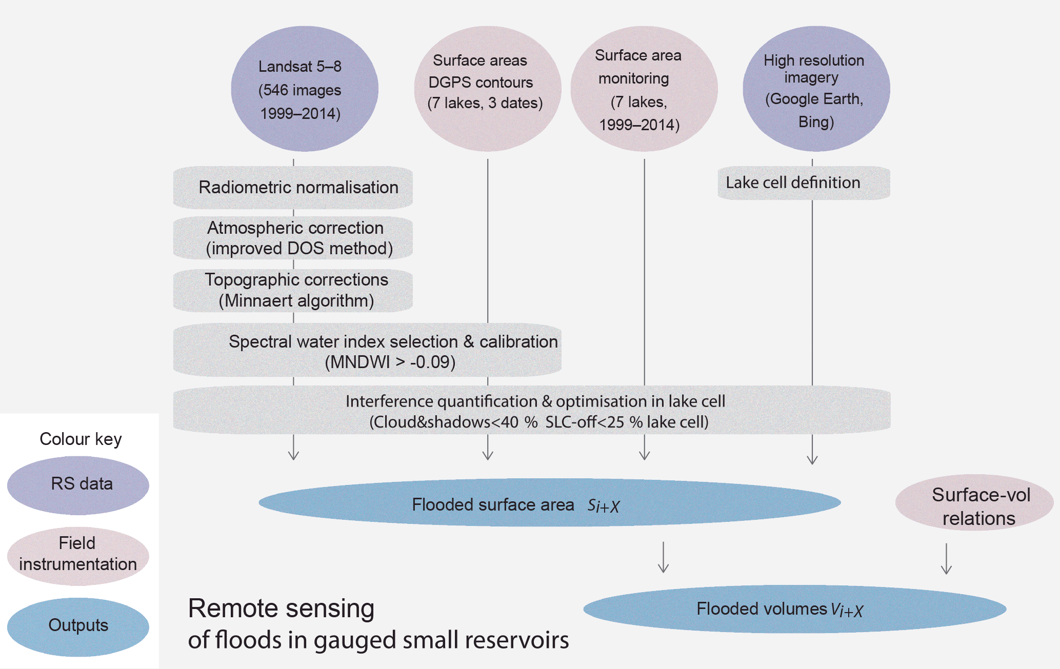
Landsat Level 1 Terrain Corrected (L1T) (orthorectified) products from USGS Earth Explorer were used here (USGS, 2018). The required radiometric (including atmospheric and topographic) corrections derived for each sensor and band combination are detailed in the Appendix. Based on data availability of Landsat images and field limnimetric data for the seven lakes, 546 Landsat 5–8 images over the period 1999–2014 were acquired and treated (Fig. 4). Lake cells to automate extraction of the flooded area were defined using freely available high-resolution imagery from Digital Globe and Astrium available in Google Earth and Bing Maps. These cells defined the maximal flooded area based on visual interpretation of geomorphological boundaries of the lake (with a 10 % buffer) and helped constrain overestimations, i.e. pixels which do not belong to the lake but which share similar reflectance profiles, such as surrounding flooded vegetation, river stretches, and temporary ponds or waterlogging.
Level 2A products corrected to land surface reflectance using the Landsat Ecosystem Disturbance Adaptive Processing System (LEDAPS) for sensors TM and ETM+ or the Landsat Surface Reflectance Code (LaSRC) for the OLI sensor were not available for our catchment and time period at the time of research. Two Landsat 8 LaSRC products now available from ESPA were acquired for 2013 to analyse the possibility of applying the water detection approach developed in this paper directly to level 2A imagery. Remotely sensed flooded areas were quantified and compared with 13 GPS contours to assess relative errors.
2.4 Spectral water indices for multi-image analysis of small water bodies
Six widely used water detection indices (Table 1) were compared to assess their suitability for monitoring floods on small reservoirs in terms of detection accuracy and threshold stability. These include the NDWI (Normalised Difference Water Index) developed by McFeeters (1996) exploiting the difference in reflectance of water in the green and NIR bands. Xu (2006) proposed a modified NDWI (MNDWI) where the NIR band was substituted by the SWIR band to improve distinction of built-up features over water. In parallel, Lacaux et al. (2007) developed the NDPI (Normalised Difference Pond Index) which also exploits the low reflectance of water in SWIR and its contrast with the green band. The NDPI is effectively the opposite of the MNDWI and was therefore not investigated separately. Gao (1996) developed a NDWI but using NIR and SWIR bands. Xu (2006) later defined this as the NDMI (Normalised Difference Moisture Index). The NDTI (Normalised Difference Turbidity Index) was also developed using the red and green bands, and exploits the principle that turbid water reacts like bare soils, i.e. low reflectance in green and high in red. The NDVI (Normalised Difference Vegetation Index) (Rouse et al., 1973) is one of the most well-known band ratio indexes and exploits the contrast between the peak reflectance in the infrared band and the low reflectance in the red to monitor vegetation. It has also been used to detect water bodies (Ma et al., 2007; Mohamed et al., 2004) as the index becomes positive in the presence of vegetation and negative for water bodies. Finally, the AWEI (Automated Water Extraction Index) (Feyisa et al., 2014) was empirically developed to discriminate water over several large lakes using wavelengths within five Landsat bands. Two variants exist, AWEInsh and AWEIsh, the latter being optimized to remove (urban and topographic) shadow pixels. Both can be used in succession in the presence of highly reflective areas (snow, roofs, etc.), but in this rural, semi-arid gently sloping watershed, the AWEInsh was used. For SWIR, band 5 for TM/ETM+ and band 7 for OLI were used in accordance with other studies (Ji et al., 2009; Ouma and Tateishi, 2006). For the NVDI and NDTI, values below the threshold were classified as water, and conversely for the four other indices.
2.5 Calibration and comparison of spectral water indices
The six water detection indices were calibrated on two Landsat 8 images to assess the performance and stability of each index in high waters (March 2013), and in low waters (June 2013) when greater proportions of vegetation growth, algae, and turbidity can affect water detection. A third image from May 2013 when vegetation and algae growth were evident but in reduced proportions was used to validate thresholds. Rainfall recorded over March–June 2013 ranged between 27 and 44 mm across the lakes concentrated on one event on 24 April 2013. Timed to coincide with the 16-day Landsat 8 acquisition cycle (Table 2), the lag between satellite overpass and field observation was inferior to 1 week, similar or inferior to previous studies (Annor et al., 2009; Liebe et al., 2005; Sawunyama et al., 2006).
Georeferenced GPS contours for each lake and date (Fig. 9 and Table 2) were used to calculate confusion matrices for each index, lake, and Landsat image. Classification thresholds for each index were varied in increments of 0.01, considering the observed influence of a second decimal in the thresholds (Ogilvie et al., 2015), and optimal thresholds were determined based on minimizing overall accuracy rates. The median threshold from all calibration points (i.e. seven lakes on two images) was retained as the optimal threshold for each index. The median was preferred over the mean threshold to reduce the influence of single lakes (and dates) where the optimal threshold is significantly different due to mixed reflectance issues. Similarly, an optimal inter-lake and inter-date threshold was not determined based on aggregated pixels from all lakes, as we sought to give equal weighting to each lake rather than allow large lakes to steer threshold values. This also ensured mixed pixels found across small reservoirs were better accounted for in the calibration (Jain, 2010). Spectral unmixing techniques (Van Der Meer, 1995) were not used here considering the marginal benefit (5 % increase in sub-pixel accuracy) observed in Sun et al. (2017) and the requirements to adapt the approach to deal with residual clouds and SLC gaps in multi-temporal Landsat time series.
The Percentage Deviation Area Index (PDAI, Eq. 1) (Sawunyama et al., 2006) was calculated to provide a relative measure of the spectral indices' accuracy in estimating flooded surface area remotely (SRS) compared to the field GPS measurements (SGPS). PDAI was not used for calibration as it is not a pixel-based assessment and was here shown to disguise spatial errors, i.e. over-classified pixels compensating for under-classified areas. Feyisa et al. (2014) showed that additional statistics, notably the Kappa coefficient and McNemar's test which focus on the frequency of pixels correctly and incorrectly classified, did not provide added benefit when optimizing water detection thresholds (Fisher and Danaher, 2013). Confusion matrices and PDAI errors per lake on the third validation image were then used to discuss the performance of each index and determine the optimal water detection index for these small water bodies.
2.6 Influence of clouds, shadows, and ETM+ scan-line corrector failure
Gap-fill methods designed to address the loss of pixels from SLC failure and interferences from clouds and shadows rely on nearby spatial or temporal spectral information. Suited for larger lakes and land use studies, spatial interpolation algorithms and decision tree classifications (Bédard et al., 2008; Maxwell, 2004) assume that nearby pixels share a similar reflectance profile which is not compatible with the small-scale analysis developed here (Feng et al., 2016; Zeng et al., 2013). Our objects of interest vary between 1 and 30 ha and are easily contained within a single SLC-off band or individual clouds. SLC failure led to the loss of around 22 % of pixels (Zeng et al., 2013), distributed along oblique lines ranging from 14 pixels wide at the edges to 2 at the centre (i.e. 420 to 60 m) (Maxwell, 2004).
Temporal methods (Scaramuzza et al., 2004; Zeng et al., 2013; Zhu and Woodcock, 2012, 2014) such as those employed by the USGS to provide SLC-corrected images exploit additional spectral data from another image close in time. These rely on the relative stability of pixel reflectance between images of nearby dates or at least assume “similar patterns of spectral differences between dates” (Chen et al., 2011; Zeng et al., 2013). These are again not suited to the detection of ephemeral localized changes (Yin et al., 2016; Zhu and Woodcock, 2014), such as small-scale, rapid changes in water surface area, which do not follow the same gradual pattern as nearby land use (vegetation) between successive images.
The Fmask algorithm (Zhu and Woodcock, 2012) was used here to quantify the presence of clouds and shadows over each lake on each Landsat image (details in the Appendix). Level 1 Quality Assessment bands provided by USGS now employ Cmask, a C version of this cloud detection algorithm, thereby providing comparable data (Foga et al., 2017). Errors from clouds, shadows, and SLC-off pixels were then assessed and minimized in post-processing by removing images for each lake with interferences above a determined threshold. This optimal threshold was determined by minimizing the root mean squared error (RMSE) on surface area aggregated over time (15 years) in order to give importance to both the number and quality of the Landsat observations over time, and therefore compromise between maintaining high temporal resolution and minimizing spatial errors from clouds, shadows, and SLC-off interferences. Thresholds were varied in 5 % increments and the quality of fit in terms of R2 and RMSE between remotely sensed surface area and field surface area was calculated for decreasing subsets of images. Gouazine lake (Al Ali et al., 2008; Nasri et al., 2004), which possessed both the longest time series (over 15 years) and the most accurate data and rating curves (updated six times), was used to optimize the thresholds. The approach was repeated on four other lakes (Morra, Dekikira, Guettar, Fidh Ali) to confirm the suitability of the thresholds and explore the resulting availability of suitable Landsat imagery over all lakes.
2.7 Remote monitoring of surface water dynamics and water availability
The complete method was applied to all 546 images and surface water extents were assessed for the seven small reservoirs over 1999–2014. Values affected by excessive cloud and shadow and SLC presence over each lake were removed and remaining observations were linearly interpolated over time into continuous time series of flood dynamics. Alternate smoothing and interpolation of discrete observations were shown not to improve the results (Ogilvie, 2015), considering the abrupt flood dynamics in small water bodies. These were then converted to volumes using the site-specific updated surface–volume rating curves. The mean water availability per year was calculated to assess the suitability of the approach for deriving long-term water availability data for stakeholders. Outliers were further constrained by the known initial maximum capacity of lakes. The skill of the method in reproducing surface water extent dynamics and water availability assessments over the seven reservoirs was discussed in the light of R2 and RMSE values against the extensive field-based data.
2.8 Comparison with published global water datasets
Results were compared to those obtained when using the global surface water datasets produced by Pekel et al. (2016) with 30 m Landsat imagery. These exploited original approaches based on a combination of expert systems, visual analytics, and evidential reasoning to classify pixels as water, land, or non-valid (here NA). Two-hundred monthly water history rasters produced by the European Commission Joint Research Centre (JRC) for our region of interest were downloaded through Google Earth Engine (Gorelick, 2017). Monthly surface water extent areas over 1999–2014 were extracted from the raster files for the 13 lakes used previously. Confusion matrices between three JRC images and the DGPS contours from 2013 on seven lakes were first calculated to provide pixel-based comparisons of the method's ability to detect water in the smallest reservoirs. Additionally, high spatial resolution (10 m) SPOT 5 multispectral imagery from 26 May 2013 was used to identify standing and floating vegetation on the seven lakes based on superior NDVI (Normalised Difference Vegetation Index) values and discuss the performance of the expert systems approach in pure and vegetated pixels. Monthly surface water values extracted from JRC datasets over 1999–2014 for seven small reservoirs were then compared with mean monthly surface areas based on in situ monitoring. RMSE and Nash–Sutcliffe efficiency (NSE) values on monthly surface water dynamics as well as mean annual water availability were again calculated to compare with results from our approach. In parallel, the number of NA values in monthly water history rasters within each lake grid cell were collected for each image to reduce their detrimental influence on surface water area estimates. NA values result from clouds and SLC-off interferences which are not differentiated in the JRC global water datasets.
2.9 Comparison with Sentinel-2 imagery
Sentinel-2A launched in June 2015 by the European Space Agency provides freely available multispectral imagery at 10 m spatial resolution (20 m in the SWIR band) every 10 days. Its constellation with Sentinel-2B launched in March 2017 increases temporal resolution to 5 days. Eighty-four surface reflectance products over 2015–2017 distributed by THEIA were used to quantify the performance of Sentinel-2 imagery and its combination with Landsat imagery after 2015 in terms of RMSE and NSE for daily surface water monitoring. Fifty additional Landsat 7 and Landsat 8 images were processed to surface reflectance through our treatment chain to extract flooded areas and additional field data from ongoing in situ monitoring on one lake (Gouazine) were acquired.
THEIA Sentinel-2 products include atmospheric corrections based on the MAJA (MACSS-ATCOR Joint Algorithm) treatment chain developed by CNES-CESBIO (Hagolle et al., 2015) and German DLR. These notably include 30 m topographic corrections, as did the Landsat imagery. Intensity–hue–saturation (IHS) pansharpening (Carper et al., 1990) was used on SWIR bands to allow water detection at 10 m (Du et al., 2016; Kaplan and Avdan, 2018) with the MNDWI and to compare performance with the 20 and 30 m MNDWI. The optimal MNDWI threshold on Sentinel-2 imagery was independently calibrated against k-means (unsupervised) classification (Jain, 2010) of flooded areas, and was substantially lower (−0.2) than with Landsat imagery (−0.09). Cloud masks provided by the MACCS algorithm were used directly, to reduce difficulties with the Fmask and Sen2cor methods resulting from the absence of the thermal band.
3.1 Spatial accuracy of spectral water indices in small water bodies
3.1.1 Water classification with variable thresholds (calibration)
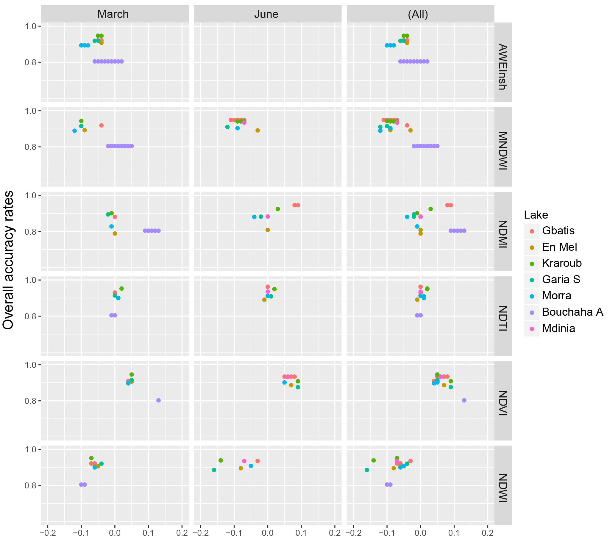
Figure 5Optimal threshold (based on overall accuracy) for each lake and index on March and June calibration images.
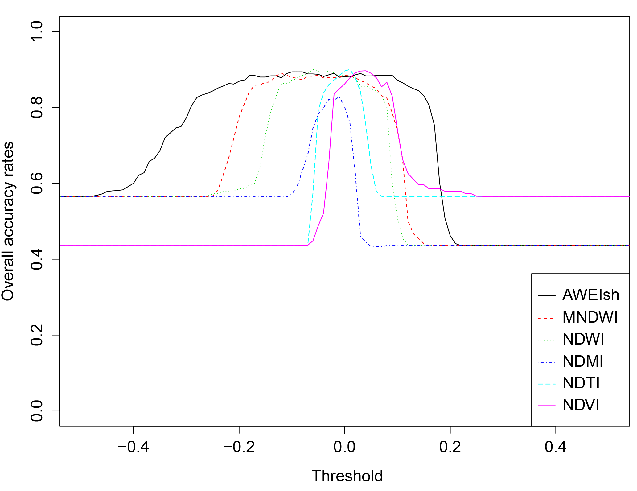
Figure 6Rate of change of overall accuracy rates for varying thresholds of MNDWI on the Landsat 8 29 March 2013 image for Lake Morra.
All six spectral water indices performed well when calibrated for a single image (March or June), achieving consistently high overall accuracy rates (Fig. 5) over 80 %. In high waters (March), associated surface area errors remain below 20 % on four out of six lakes. Even on the smallest lake (Gbatis) the PDAI values varied between 9 % and 27 % depending on the index, showing remarkable precision considering its size of 1 ha and the coarse 30 m image resolution.
In low waters (June), PDAI values degraded however for the NDVI, NDWI, and NDMI and exceeded 50 % on the smallest lake. Only the MNDWI and NDTI maintained PDAI rates below 25 % for all lakes. In the dry season, lower water levels, greater algae, and vegetation growth make accurate discrimination more complex (Ji et al., 2009). Smaller lakes intrinsically have a higher proportion of mixed pixels and shallow waters (Mialhe et al., 2008) where the spectral reflectance is a combination of water, soil, and vegetation. The coarse resolution exacerbates these errors due to the proportionally greater influence of a single misclassified pixel on the result (1 ha corresponds to a little more than 9 pixels).
The NDVI, which suffers from an inability to correctly distinguish vegetation from flooded vegetation, sees its performance diminish accordingly. The NDMI on the other hand performed better in low waters, coherent with its objective to detect moisture and all types of water. Thanks to the middle infrared band which penetrates water less and is less affected by turbidity and vegetation in the water, NDMI was able to detect the two smallest lakes, but low user accuracy led to gross PDAI errors, as it overclassified many vegetated pixels. MNDWI and NDTI fared the best with these smaller reservoirs (e.g. Gbatis) due to their ability to detect turbid waters and distinguish flooded vegetation over wet vegetation on land.
AWEI performed well on the first image, but the index failed on the other images, with overall accuracies falling below 60 % on four lakes. These were here related to inherent discrepancies in the radiometric corrections apparently amplified by the nature of the AWEI equation, rather than contained as with other normalized band ratio indices. Normalizing reflectance values between the 546 images may help reduce these issues, but as a result AWEI was not considered for the semi-automation of this method. Furthermore, Jiang et al. (2014) showed that MNDWI outperformed AWEI when extracting narrow water bodies on Landsat.
3.1.2 Water classification with fixed thresholds (validation)
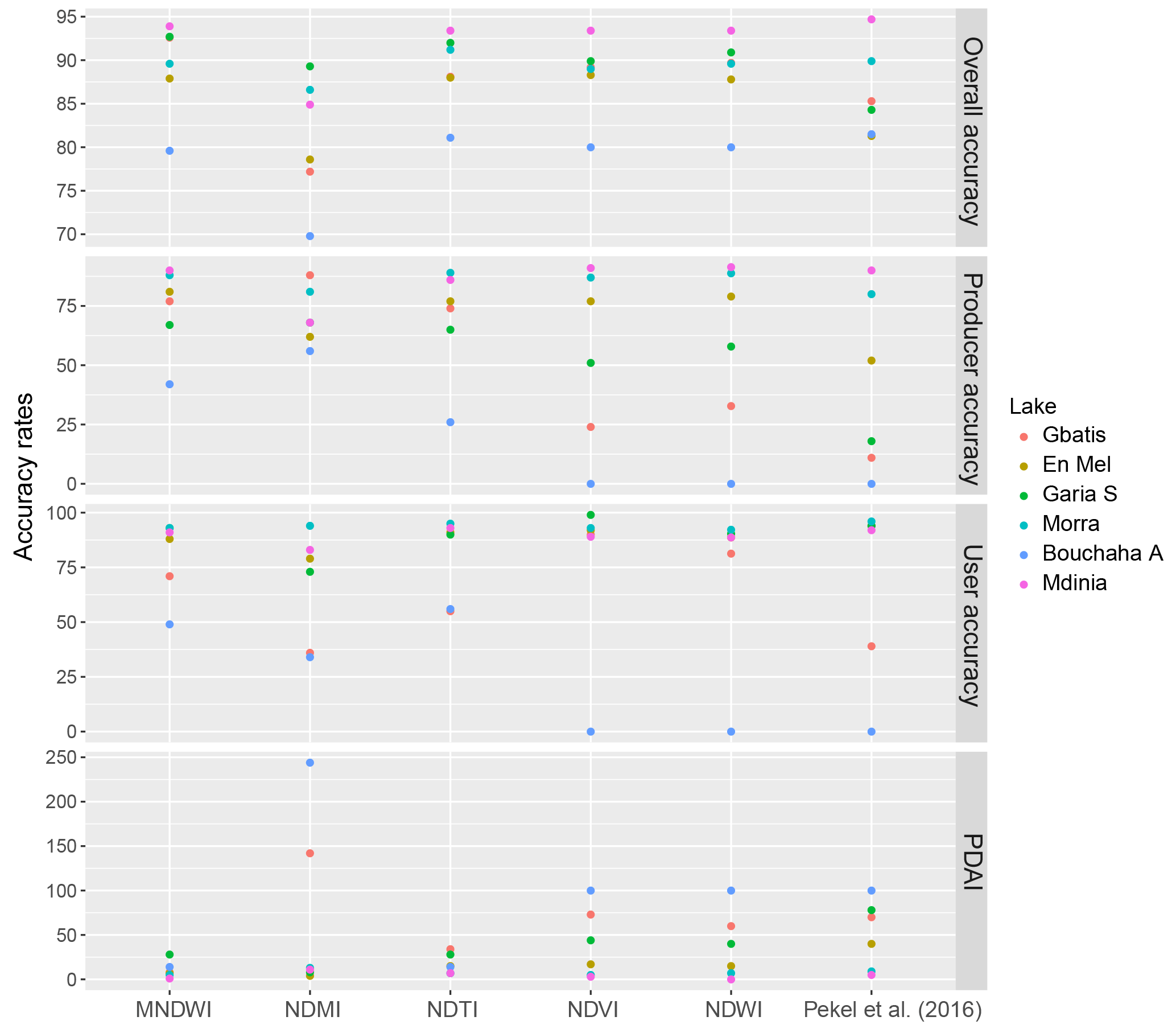
Figure 7Accuracy and error values for five spectral water indices and the Pekel et al. (2016) expert systems approach on the May validation image.
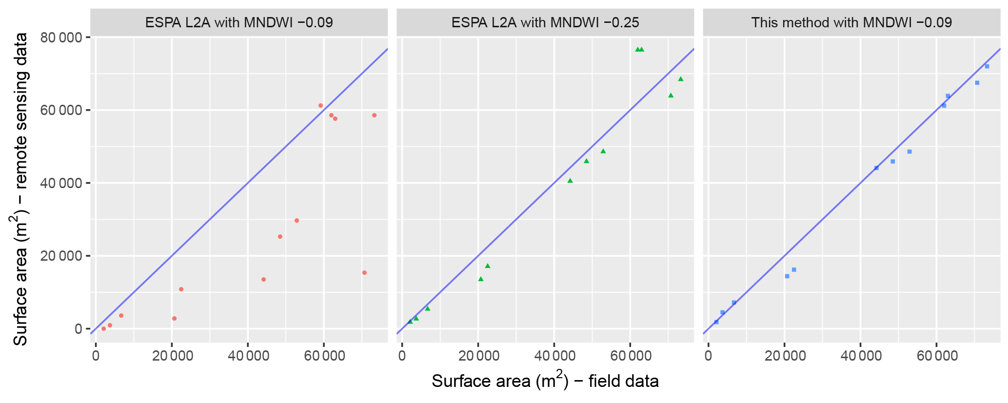
Figure 8Remotely sensed surface areas with MNDWI on Landsat ESPA surface reflectance products and Landsat surface reflectance through our treatment chain vs. field data (13 DGPS contours) in May and June 2013.
The optimal threshold determined from the March and June images on seven lakes was used in validation on a third image (May). Accuracy rates remained high for MNDWI and NDTI, but reduced significantly for the three other indices (Fig. 7). Issues of shallow waters and vegetation were again prevalent here and even an image-specific threshold could only minimize omission and commission errors to 50 % with the NDVI, resulting in a PDAI of 46 %.
The stability of the individual thresholds (Fig. 5) combines with the sensitivity to threshold change (Fig. 6) to determine the amplitude of the errors when using fixed thresholds. A marginal shift in threshold due to shallow waters and abundant algae will then introduce larger errors and omission rates, with the NDVI and NDWI reaching 76 % and 100 % on the smallest lakes. The significant rate of change observed highlighted that thresholds must be optimized up to two decimals. The MNDWI achieved better accuracies on these small lakes and achieved consistently the lowest PDAI errors, as a result of the lower rate of change in the MNDWI over the NDTI (Fig. 6).
These results confirm firstly its suitability over other band ratio indices on the smallest lakes, in line with results on larger water bodies (Feyisa et al., 2014; Ji et al., 2015; Jiang et al., 2014; Ogilvie et al., 2015). Applied across seven lakes and three images, the method yields a R2 Pearson correlation coefficient of 0.99 and low RMSE errors, confirming secondly that a fixed-threshold MNDWI can be used to study over time lakes from 1 ha with 30 m Landsat images (Table 2). Surface area errors ranged from 1 % to 28 % (mean 10.5 %, SD 8.7 %) with some underestimations observed due to undetected narrow inlets on certain lakes. On the smallest lakes (Bouchaha A and Gbatis) however errors reached only 14 % and 8 %. In the dry season, Bouchaha A reduced to only 0.2 ha; therefore, PDAI error reached 50 % with all indices, which is to be expected as it corresponds to just over 2 Landsat 30 m pixels.
Optimizing thresholds for each lake and image individually can reduce PDAI errors below 5 %, highlighting the potential for further improvements by developing (unsupervised) classification methods capable of being used over numerous locations and images reliably and efficiently (in terms of CPU and user input). Optimizing thresholds for each lake but not each image only improved performance on certain small lakes.
Comparison between the Landsat surface reflectance products (level 2A) provided by ESPA and 13 DGPS contours revealed that lake surface areas are significantly underestimated on all lakes, except Mdinia (Fig. 8) when using the MNDWI threshold determined here (−0.09). RMSE reaches 22 000 m2 with the L2A products compared to 3200 m2 with surface reflectance products through our treatment chain, largely resulting from underestimation in small lakes. Lowering the MNDWI threshold further (to −0.25) to increase the classification of water with standing vegetation can reduce RMSE to 7000 m2, but leads to overestimations (over 20 %) on large lakes such as Mdinia. Considering the good performance of the atmospheric corrections provided by ESPA's 6S Landsat Surface Reflectance Code (6S-LaSRC) (Doxani et al., 2018; Vermote et al., 2016), the greater dispersion in the reflectance values observed may be explained by the finer topographic corrections performed in our treatment chain (30 m SRTM vs. 1 km GCM DEM by LaSRC), necessary when monitoring small water bodies.
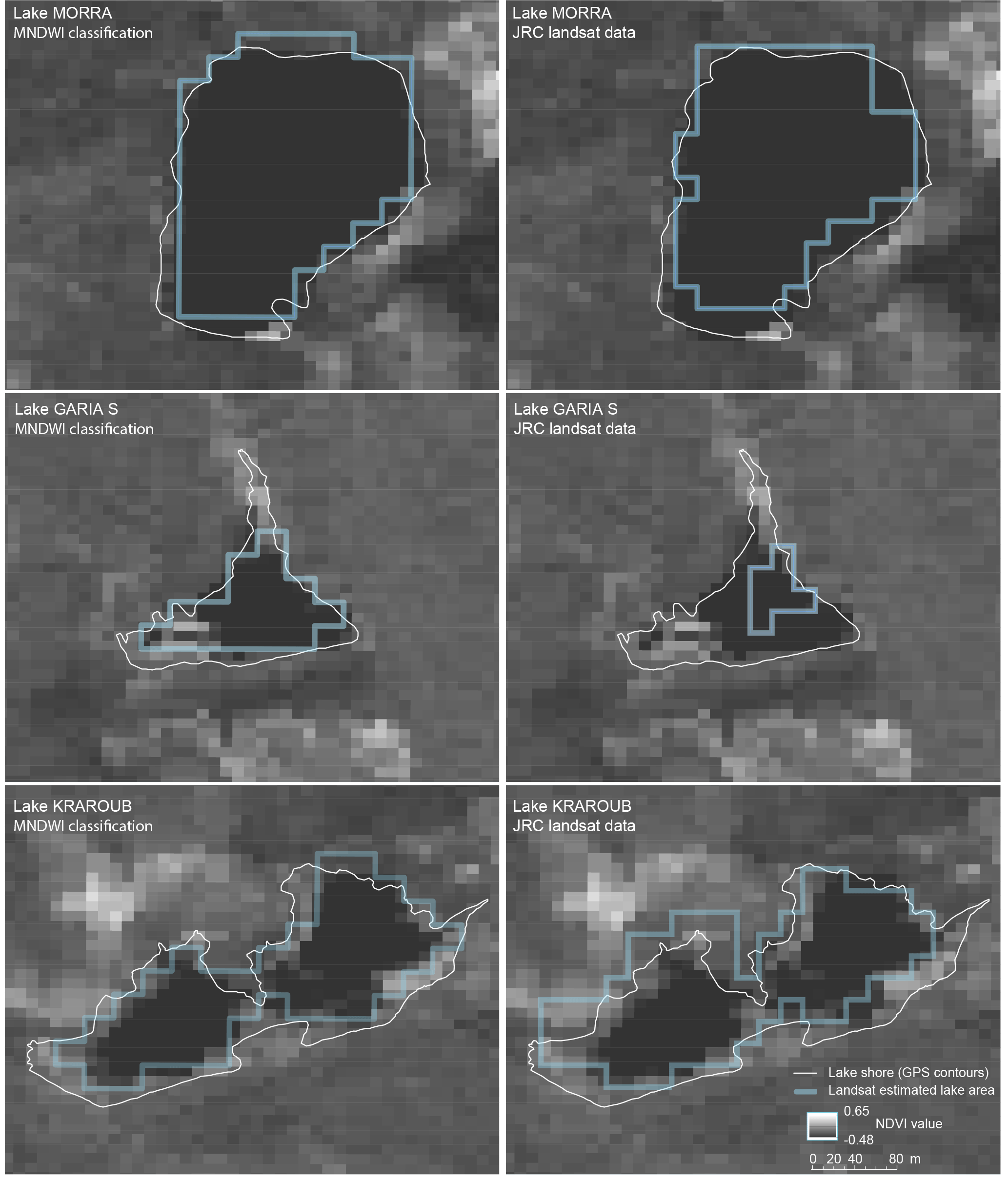
Figure 9Comparison of surface water classification from the MNDWI approach and JRC data against DGPS contours and SPOT 5 NDVI maps for three lakes in May 2013.
3.1.3 Comparison with previous approaches
Previous studies to map small reservoirs yielded PDAI errors of 10 % to 50 % on lakes in the range 1.5–5 ha and with image-specific thresholds (Liebe et al., 2005; Sawunyama et al., 2006). Errors in this study remained minimal even on lakes of this size despite the same spatial resolution of the images, pointing to the improved ability of indices in detecting mixed pixels caused by shallow waters. Including mixed pixels from small reservoirs in the calibration also improved performance (Jain, 2010; Ji et al., 2009) and led to a slightly lower threshold (−0.09). The MNDWI threshold for water detection is often near 0, but here a value close to that found in wetlands (Ogilvie et al., 2015) with similar mixed spectral profiles was determined.
Confusion matrices performed on the JRC monthly surface water rasters (Pekel et al., 2016) confirmed their excellent performance on larger lakes in high waters (e.g. Morra, Mdinia), with the PDAI under 10 % and overall accuracies near 90 %. Overall accuracy values remained high (>80 %) on other lakes, due to the large number of non-water pixels correctly classified in each lake cell, but water omission errors (i.e. producer accuracy) on the smaller lakes (under 5 ha) were substantial, rising in some cases to over 50 % (Fig. 7). Commission errors remained minimal (10 % on average), indicating that the expert system approach suffered from the inability to detect all types of water, rather than from overdetection. Confusion matrices on the June images confirmed the progressive decline in accuracy as water reduces and the presence of flooded vegetation, algae, and shallow waters increases. In June, overall accuracy rates declined and the PDAI for instance rose from 9.1 % to 18.7 % on Morra and up to 74.7 % on Kraroub, where significant algae and vegetation growth was observed. In comparison, the MNDWI, designed to detect mixed water reflectance, led to a 7.1 % PDAI on this 5 ha lake. Across all seven lakes, omission errors in JRC datasets reached 32 % in high waters and 41 % in shallow waters. These are substantially higher than values provided in Pekel et al. (2016) (23 % for seasonal water bodies in Landsat 8) and in Mueller et al. (2016) (12 % in small water bodies and 26 % where water and vegetation mix). These suggest that the validation approach which uses sample pixels with a “high probability of water occurrence” within 1∘ tiles (Pekel et al., 2016) may introduce a bias towards larger, near-permanent water bodies, which also contained greater proportions of clear-water pixels.
NDVI maps created from high-resolution (10 m) SPOT imagery confirmed the accurate detection of pure water pixels by both methods and illustrate the difficulties with the JRC datasets where lakes include standing or floating vegetation (Fig. 9). The lake fringes are notably excluded by the JRC approach, which on larger lakes such as Morra and Mdinia leads to minor underestimation of the flooded area. However, on lake Garia S, where vegetation is observed on much of the west of the lake, this leads to substantial underestimations (PDAI = 80 %). NDVI maps also highlight additional pure water pixels in the south of Garia S and En Mel lakes which are excluded by the expert systems approach. Conversely, on lake Kraroub, the JRC datasets included vegetated pixels in May 2013 but not in June 2013. Though results point largely to difficulties in detecting shallow waters where reflectance is affected by vegetation and turbidity, other factors influencing the JRC approach such as terrain shadows and lake morphology could not be excluded here. The good performance on Kraroub in May 2013 confirms that in some situations, the expert systems approach is capable of reaching its goal of detecting water even with variable “chlorophyll concentration, total suspended solids and coloured dissolved organic matter load” (Pekel et al., 2016), but not systematically.
3.2 Influence of clouds, shadows, and SLC-off pixels on multi-temporal analysis
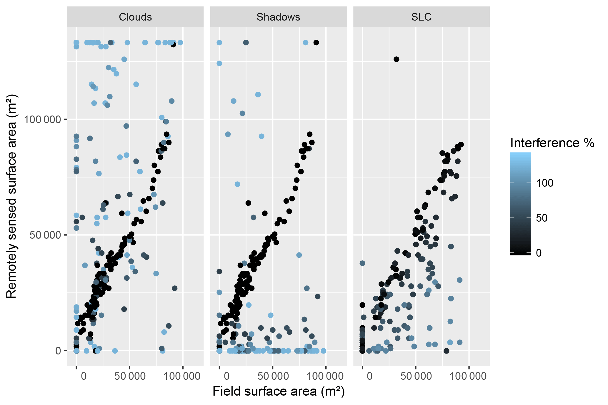
Figure 10Errors due to interference from clouds, shadows, and SLC-off percentage across the Gouazine lake cell.
3.2.1 Interference from clouds, shadows, and SLC-off
The influence of clouds, shadows, and SLC failure on estimated flooded areas from Landsat imagery over 1999–2014 is illustrated in Figs. 10 and 11 based on field data from one small reservoir. Detected on 28 % of the 546 Landsat images, clouds lead essentially to commission errors (false positives) and overestimation, as a result of visible wavelengths being reflected while much of the electromagnetic energy is absorbed by the droplets in clouds. Their effect was not systematic and proportional (Fig. 11), as shown by underestimations in 30 % of cases where clouds were detected across the whole lake cell. The diversity in the nature and properties (temperature, thickness, water content, etc.) of clouds is indeed firstly responsible for the heterogeneous reflectance observed and the resulting classification difficulties. The influence of shadows is more moderate and less frequent, responsible for overestimations in only 5 % of images. This results partly from the greater difficulties in discriminating shadows and the overlap from clouds. Pixel loss from SLC failure varies across Landsat tiles, and for a given lake, 30 % of the 287 Landsat 7 SLC-off images suffered from minor pixel loss (<10 %). SLC-off pixel loss led to a systematic underestimation of flooded areas, on average by 35 % (Fig. 11).
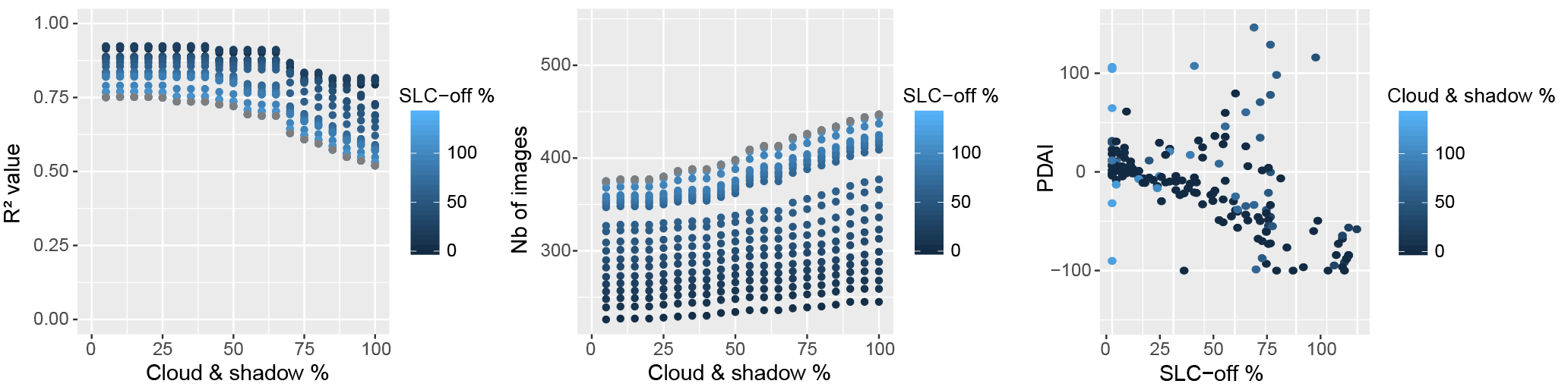
Figure 11Change in R2 (between field and remotely sensed surface areas), remaining number of Landsat scenes, and PDAI for increasing percentages of SLC-off and cloud and shadow pixels tolerated (Lake Gouazine).
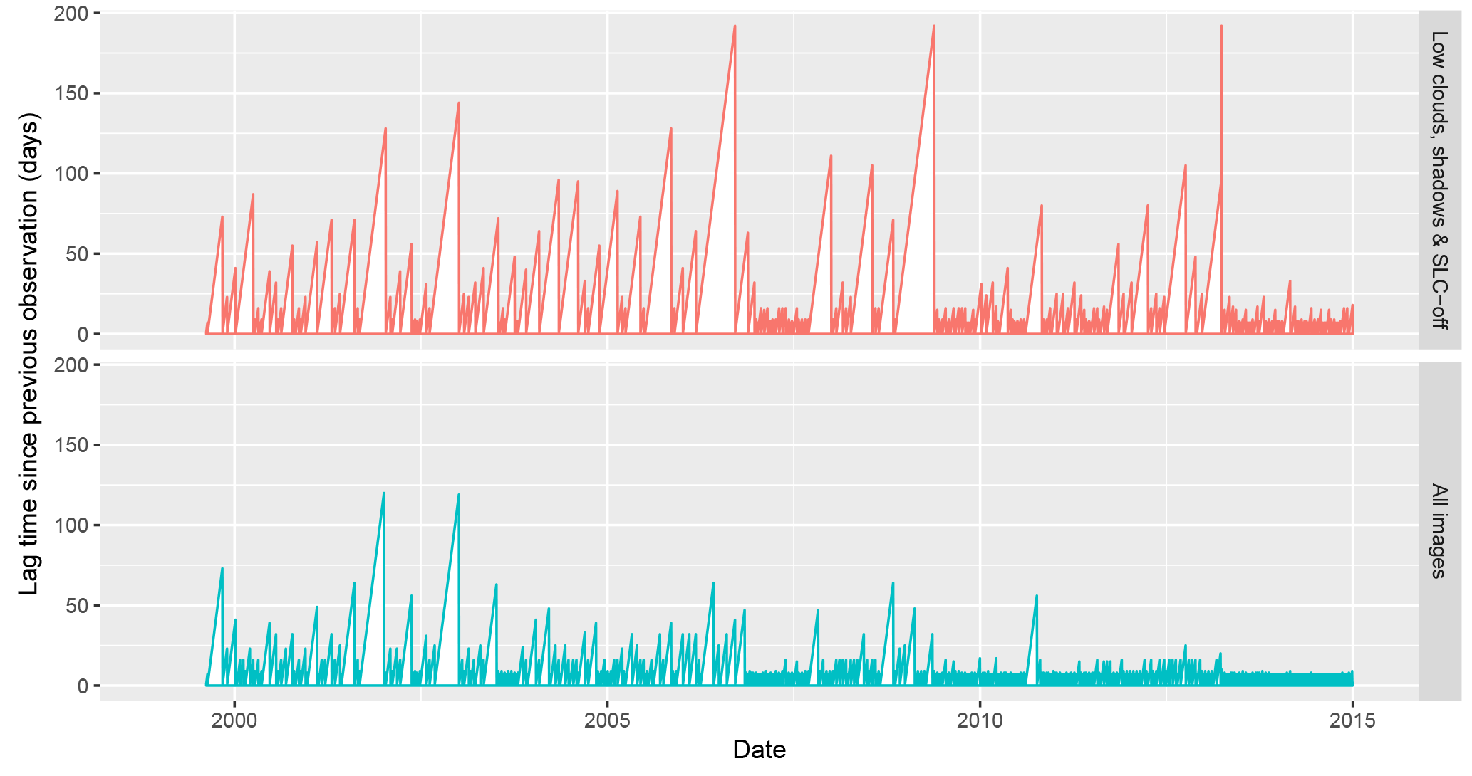
Figure 12Lag time between successive Landsat images, based on all images available and after optimization to reduce clouds, shadows, and SLC-off interferences.
3.2.2 Optimizing image availability vs. interferences
Optimizing on R2 tends towards removing all cloud and SLC interferences, and therefore reduces the number of available observations. Considering the objective of hydrological monitoring and maintaining sufficient temporal repetitivity, images with up to 25 % SLC-off pixels and 40 % cloud and shadow pixels over the studied lake cell were retained here. These thresholds were found to minimize the mean squared error on surface area aggregated over 15 years, which gives importance to both the number and quality of the Landsat observations over time.
This calibration removed a significant 51 % of images, leaving on average 282±27 Landsat images suitable for observations across these seven small reservoirs (Table 3). This equates to 1.5 images month−1 over the 1999–2014 period studied, though these are unevenly distributed as seen in Fig. 12, due partly to low overall cloud cover between March 2013 and December 2014 over our area of interest. The acquisition cycle of Landsat 7 is also staggered by 8 days compared to Landsat 5 and 8, leading to a revisit frequency of up to 8 days. The Merguellil catchment is located at the overlap of two paths visited at a 7-day interval, further increasing availability.
Significantly when studying one lake, 59 % of the Landsat 7 post-2003 images were discarded due to SLC-off pixels, and 31 % of all Landsat images were removed due to excessive cloud presence. Variations between lakes in the number of images available were high when using the same thresholds, due to greater cloud presence on higher-altitude lakes (Morra) as well as the irregular SLC interference detailed earlier. These confirm the value of lake-specific cloud detection to account for the scale of small reservoirs (i.e. a 0.1 km2 area within a 33 300 km2 Landsat 8 tile, i.e. 0.0003 %). In other catchments, proximity to coastal areas and more pronounced orography may increase the proportion of images affected by clouds.
3.3 Remote monitoring of surface water dynamics in small reservoirs
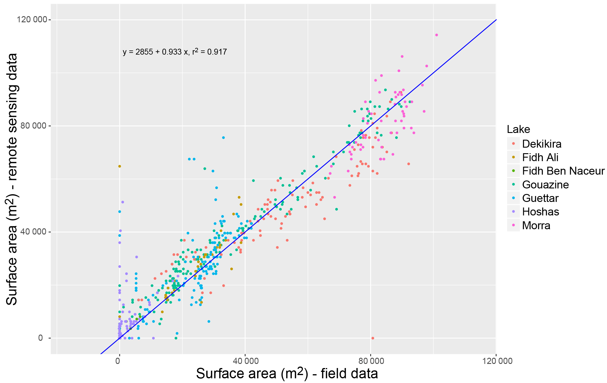
Figure 13Remotely sensed surface areas with the MNDWI on Landsat imagery vs. field data over 1999–2014 across all seven lakes.
Results from this semi-automated method applied across 546 Landsat images (1999–2014) and seven lakes yielded a strong correlation (R2=0.92) between remotely sensed flood areas and field data (Fig. 13). Confirming its excellent performance in terms of accuracy and stability across reservoirs and over several years, the results also substantiate the method's ability to be used across multiple sensors, notably Landsat 8 OLI with Landsat 7 ETM+ and Landsat 5 TM, in line with what Vogelmann et al. (2001) showed on TM and ETM+. On larger lakes with long-term and accurate time series such as Gouazine, R2 reached 0.95 with an RMSE of 6800 m2 (Table 3). When accounting for the lake size, this equates to a median relative (PDAI) error of 11 % (Fig. 14).
Landsat observations provided here accurate insights into the surface water extent dynamics, closely reproducing flood peaks and declines notably (Fig. 15). Reduced image availability due to clouds, shadows, and SLC-off however prevented accurate representation (interpolation) of the steep flood rises associated with intense rapid floods as opposed to the more gradual declines, easier to interpolate. As seen in Figs. 10 and 11, increasing the allowance of clouds, shadows, and SLC-off pixels to raise image availability leads to a decline in R2 and a rise in the PDAI. Conversely, single outliers remain, but reducing cloud, shadows, and SLC thresholds was shown not to remove these larger classification errors. These outliers are due to the inherent uncertainties in the method, partly incomplete detection of clouds, and classification difficulties (e.g. overestimation as a result of detecting water flow in the tributaries or peripheral flooding due to cells being defined broadly to account for exceptional flood volumes). Stage-derived surface areas are subject to rising uncertainty after 2008 due to the obsolescence of the rating curve (estimated at 2300 m2 from Fig. 3), but Fig. 16 does not signal a marked shift in the rating curve.
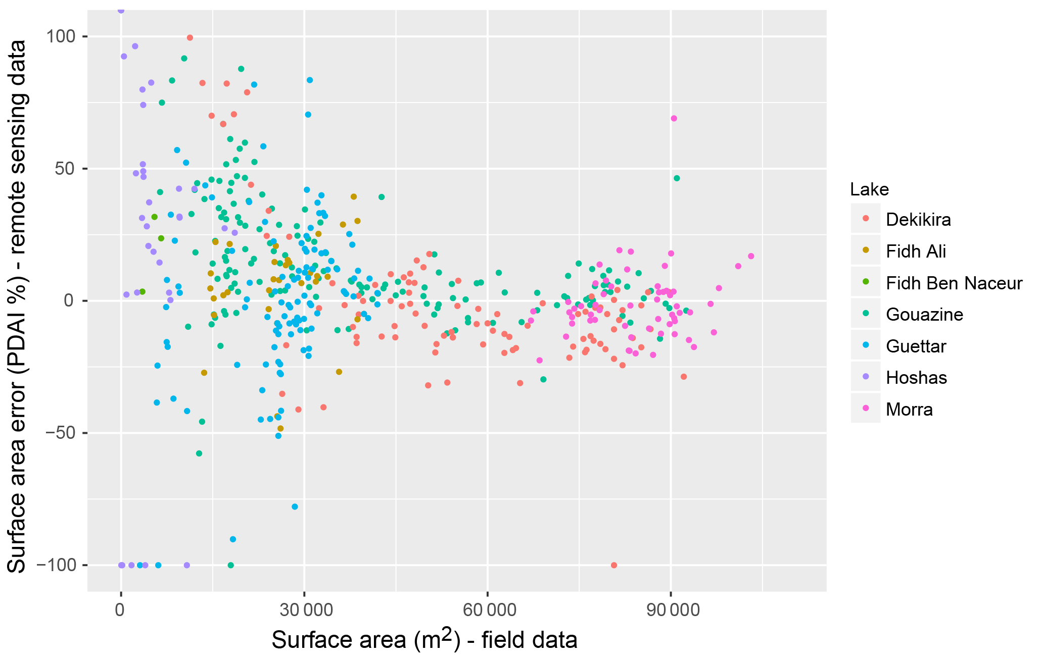
Figure 14Surface area error (in PDAI %) from remote sensing data against field data for seven lakes.
3.3.1 Greater errors on small lakes
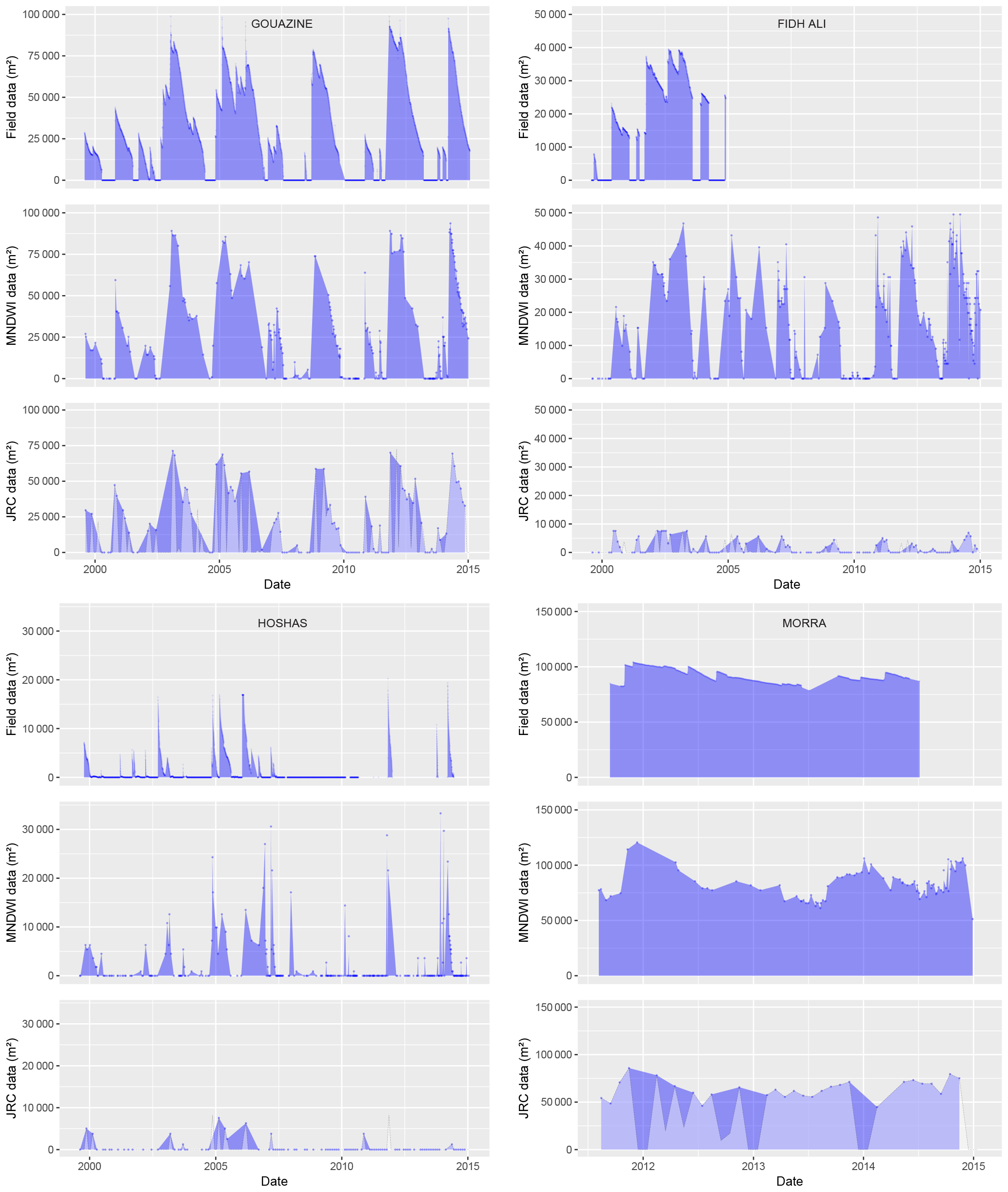
Figure 15Surface water extent dynamics from field data and remote sensing over 1999–2015 for four lakes. JRC data (Pekel et al., 2016) are filtered to images with less than 25 % NA over the lake cell (the complete JRC datasets are represented in pale blue).
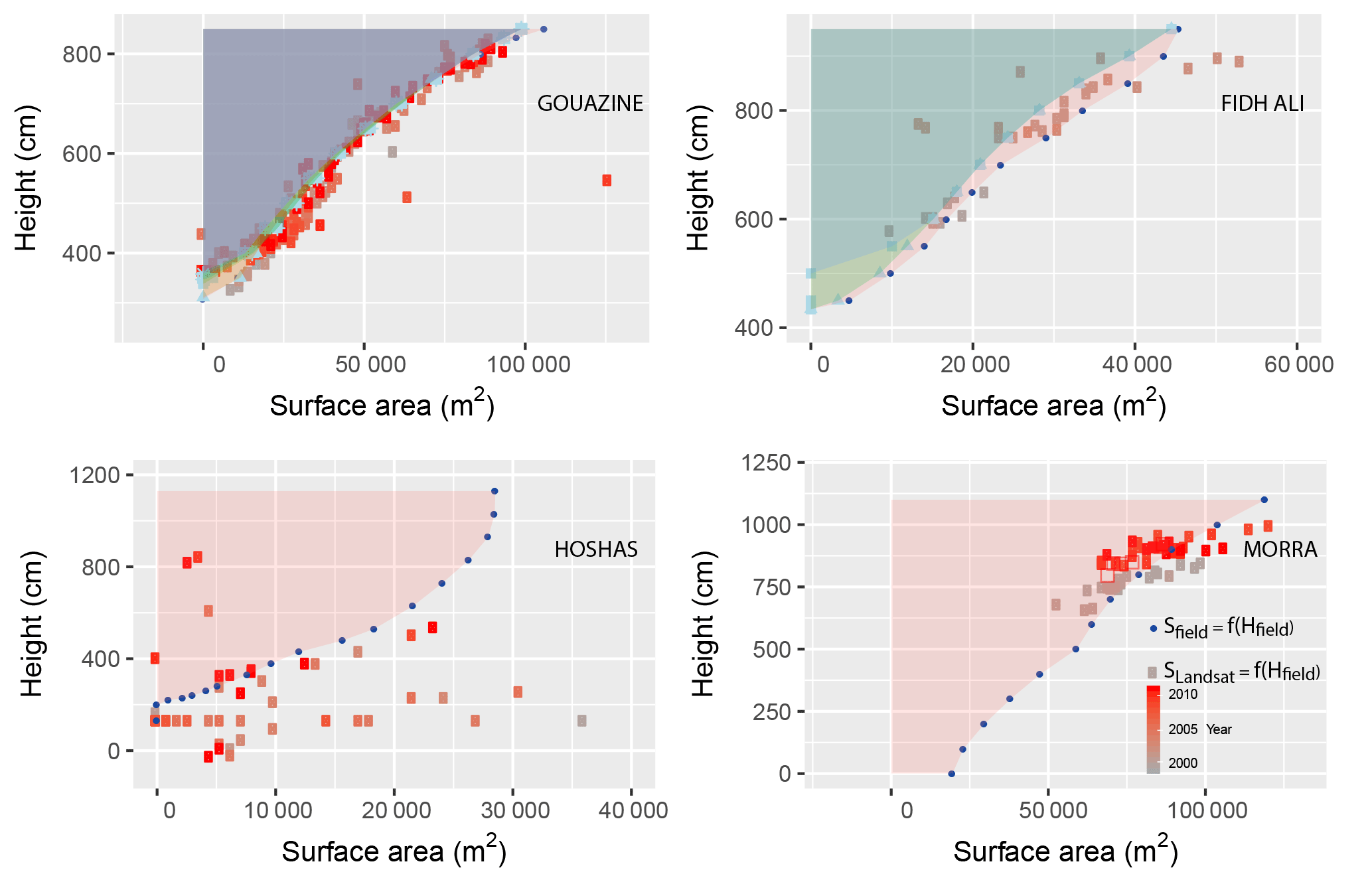
Figure 16Comparison of field-based H–S rating curves and the H–S rating curves that could be established based on Landsat surface water observations over 1999–2014.
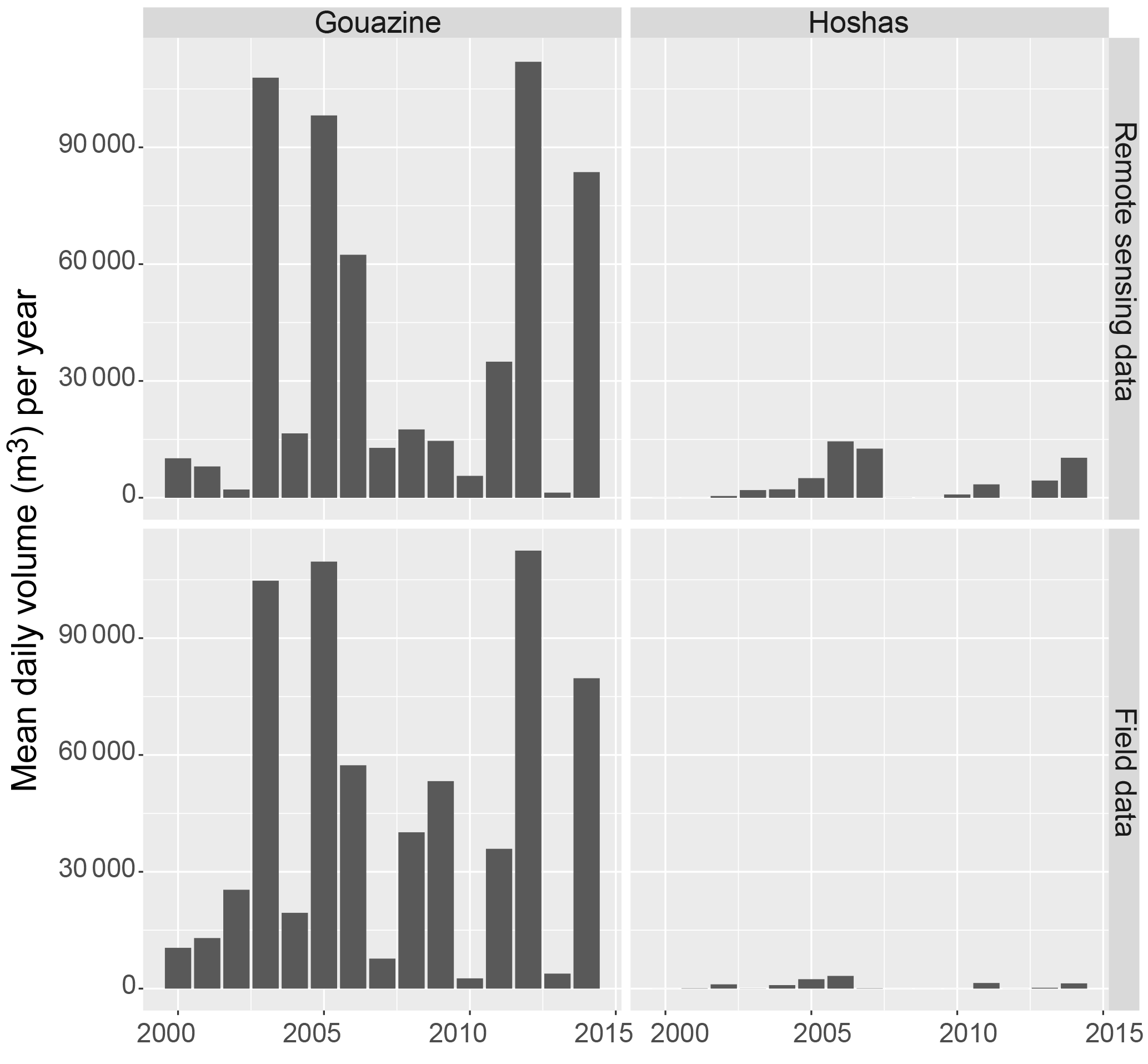
Figure 17Annual mean volumes from field data and remote sensing data over 1999–2015 for two lakes .
On smaller lakes, the influence of incorrectly detected pixels is proportionally greater due to the low spatial resolution and reduced pixel numbers. Mean PDAI rises from 13 % to 27 % on surface areas under 3 ha and scattering is reflected in the reduced NSE skill values (Fig. 14 and Table 3). On Hoshas, this is exacerbated by the numerous empty periods and the greater mathematical influence on R2 of minor classification noise. Errors are also proportionally greater at the lower part of the H–S rating curves. Figure 16 highlights on Hoshas the multiple classification errors (overestimation and nondetection) and the observed dispersion confirms that errors are only partially affected by the absence of prior rating curves. Over a reduced period (2011–2014) where the lake was regularly flooded and data confidence is greater, R2 for Hoshas rises to 0.77. Smaller lakes also suffer from greater classification difficulties, discussed in calibration of indices, due to more heterogeneous pixels where soil, vegetation, and water reflectances overlap. Threshold calibration of our MNDWI led here to a minor overestimation for the lowest water levels, as seen in Fig. 14 and for Fidh Ali and low flood levels in Gouazine in Fig. 13. In absolute terms, however, mean error remains restricted to 9300 m2 for both small and larger lakes.
3.3.2 Dealing with rapid flood declines
On these smaller lakes, the method continues in many cases to be able to derive time series reproducing surface water dynamics, notably highlighting drought periods and the minor flooded areas (e.g. Fidh Ali in Fig. 15). However, the reduced amplitude of the flood and crucially the rapid decline can lead to difficulties. Out of seven events on the smallest lakes (Fidh Ben Nasseur and Hoshas), two minor events (0.5 ha flood) were completely undetected and two were detected after surface area had declined by 50 %. On these lakes, 1 ha floods were completely infiltrated and evaporated within 21 days. Figure 15 also illustrates the difficulty in interpolating points with variable and non-negligible time lag into a hydrologically coherent daily time series. Available observations remained however relatively accurate on Fidh Ben Nasseur (R2=0.91), showing the potential of the method even on the smallest lakes (<1 ha), subject to sufficient temporal resolution. The launches of Sentinel-2A in 2015 and Sentinel-2B in 2017 provide increased opportunities to monitor with high temporal resolution rapid flood dynamics in small reservoirs, discussed in Sect. 3.6.
3.3.3 Reduced surface water amplitudes
On the largest lake studied here (Morra), Normalised root mean square error (NRMSE) remains moderate (14 %); however, the low R2 translates the difficulties in extracting consistent flood trends from the remote sensing data (Fig. 15). GPS contours revealed a 9000 m2 error associated with the stage–surface rating curve (Fig. 3) which has not been updated for over 20 years due to the lake remaining flooded through the year and the access difficulties in performing bathymetric surveys. Comparing remotely sensed surface areas with field stage readings (Fig. 16) illustrates the potential of using Landsat observations to define and correct hypsometric relationships in small water bodies, such as Gouazine and Morra. On Hoshas, the dispersion in the values indicates that errors are only marginally influenced by the absence of prior rating curves and confirms the presence of remote sensing uncertainties. On Morra, Fig. 16 illustrates the inadequacy of the rating curve, and notably its inferior slope which leads to a reduction in the amplitude of flooded surface area variations. A shift in the rating curve is also apparent during the late 2000s, resulting either from a major silting event or from a shift in the placement of the ladder. Using the Landsat observations after 2011 to define a new rating curve leads to a closer match between stage-converted surface area and remotely sensed surface area. This is expected considering the bias it introduces, but here RMSE reduces only marginally by 10 %, indicating that the rating curve errors are not sufficient to explain the low performance observed. This may be partly explained by the morphology of this large deep lake, where the uncertainties of the remote sensing method (combined with the rating curve) are significant compared to the amplitude of the surface area variations (80 000–100 000 m2 on Morra against 0–90 000 m2 on Gouazine). Accordingly, it is not only the spatial resolution and number of pixels but also the amplitude of variations in the flooded surface area over time which determine by how much remote sensing of surface water extent is affected by uncertainties and scattering.
3.4 Remote assessment of long-term water availability in small reservoirs
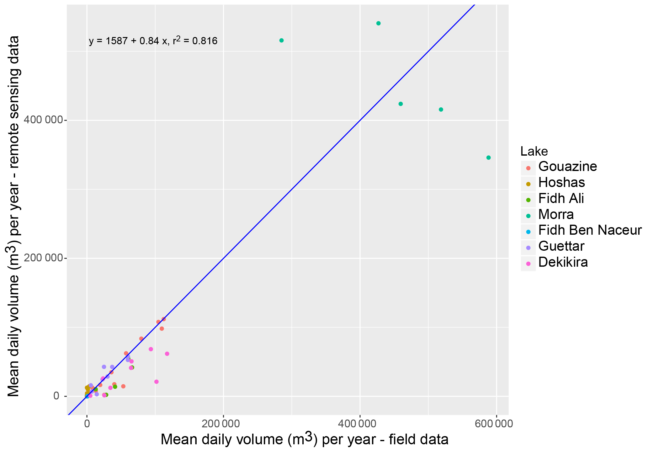
Figure 18Mean daily volume per year with MNDWI on Landsat imagery vs. field data over 1999–2014 across all seven lakes.
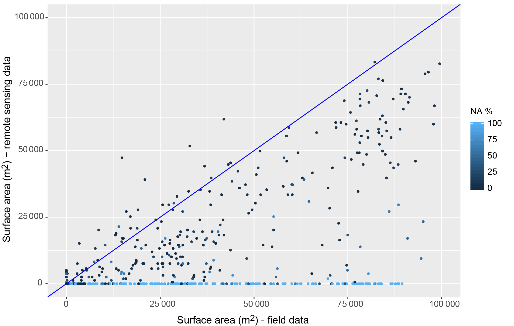
Figure 19Remotely sensed surface areas with global surface water datasets (Pekel et al., 2016) vs. field data over 1999–2014 across all seven lakes. The percentage of NA pixels was calculated over each lake cell.
Daily time series of surface area aggregated and converted into mean annual surface volumes are shown in Fig. 17. The fit with the mean volume assessed from stage data is again excellent for Gouazine (R2=0.91) (Table 3). On other lakes, the absence of stage data over several years limited the number of values which could be compared, but for available years Fig. 18 indicates a good overall fit (R2=0.82). The method therefore provides a valuable tool to assess and compare water resources between years and lakes. Transposed to multiple ungauged lakes where no hypsometric relationships are available, this approach can highlight the significant variability in terms of inter-lake and inter-annual water availability (Ogilvie et al., 2016a). This information may then help farmers and stakeholders quantify the risk of agricultural drought and optimize their agricultural practices and investments accordingly. In the Merguellil catchment, water availability patterns are being spatially confronted with agricultural production to explore to what extent hydrological constraints suffice in explaining agricultural water patterns and what additional socio-economic factors must be accounted for.
R2 values increased for certain lakes as a result of the smoothing of the method's uncertainties (e.g. Guettar and Hoshas), but conversely reduced on other lakes (e.g. Dekikira). Interpolation over time between discrete Landsat observations can lead single outliers to reduce overall performance if they are not rapidly corrected by a subsequent observation. The influence of outliers is then variable and depends on the lag between successive correct observations. Similarly, all observations do not carry the same importance when assessing mean annual volumes. Landsat observations close to the peak of an event are accordingly more important than observations during dry periods or the (gradual) decline of flooded areas, which can be more easily interpolated.

Figure 20Surface area error (in PDAI %) from global surface water datasets (Pekel et al., 2016) against field data for seven lakes.
3.5 Comparison with published global datasets
Analysis of available monthly surface water datasets (Pekel et al., 2016) against field data for seven lakes over up to 15 years (1999–2014) highlighted firstly the incidence of NA pixels and the necessity to assess and remove NA pixels above individual lakes to reduce underestimations (Fig. 19) and reproduce coherent flood dynamics (Fig. 15). Filtering out images with over 25 % NA values per lake cell led to optimal RMSE errors and is coherent with the SLC threshold determined with our approach. After NA removal, NSE across all seven lakes rose from 0.39 to 0.78, but Fig. 20 confirms the residual difficulties, consistent with the omission errors identified on single JRC water history rasters (Figs. 7 and 9). Mean RMSE reaches 22 500 m2 and removing all NAs only improves RMSE further to 21 800 m2 compared to 9300 m2 with the MNDWI approach. On small lakes under 5 ha which present greater shallow waters and flooded vegetation, PDAI errors are proportionally more important and reach 61 % on average. On Fidh Ali (Fig. 15), difficulties due to the significant vegetation in the lake lead to vast underestimations and fail to detect certain floods completely. On surface areas over 5 ha, the PDAI remains high around 35 % and interestingly continues to underestimate surface water areas. These result from omission errors during summer months due to vegetation growth in permanent lakes as well as undetected vegetated areas on the fringes inundated during large floods. Figure 15 highlights the valuable insights into the general flood dynamics that can be extracted from the JRC datasets on larger lakes such as Gouazine and Morra, though omission errors remain apparent in the underestimated flood peaks.
These classification inaccuracies are further exacerbated by the limited number of observations. After NA removal, JRC monthly water history sets provide for instance 99 exploitable images over 1999–2014 on Gouazine, compared to 269 when using the complete L5, L7, and L8 archives filtered for clouds, shadows, and SLC failure (Figs. 11 and 12). The greater temporal resolution allows better detection of dry spells, multiple flood peaks, timing of flood peaks, and more coherent flood rises and declines as seen on Gouazine, while on the small Hoshas lake two floods in 2013–2014 are otherwise undetected with JRC datasets (Fig. 15). These difficulties also have implications for the accuracy of maximum extent estimates, and though median underestimation is 41 %, the spread in the error (Fig. 20), even for larger lakes, prevents systematic corrections. Surface area inaccuracies on small lakes in JRC datasets also degrade water resource assessments for farmers or water balances for hydrologists, with for instance Gouazine RMSE on mean water availability increasing by 24 % to 17 800 m3.
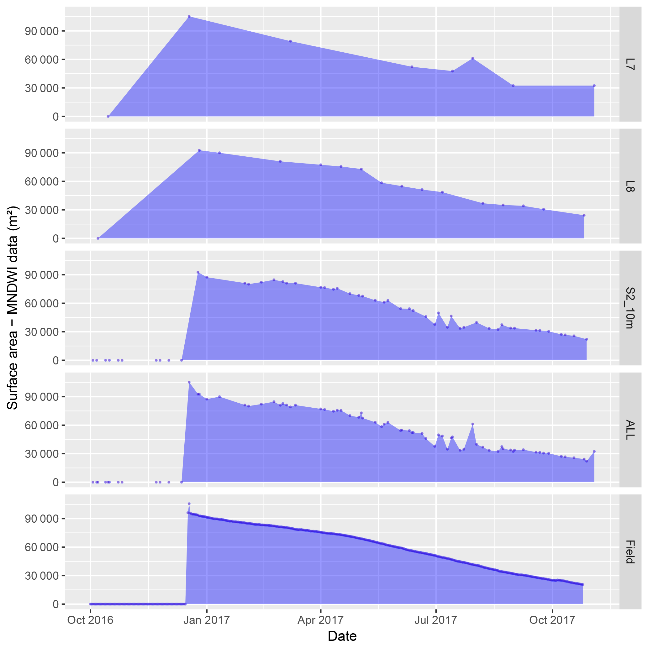
Figure 21Surface water extent dynamics from Sentinel-2 and Landsat 7 and 8 and field data over 2016–2017 on lake Gouazine.
3.6 Comparison with Sentinel-2 imagery
Sentinel-2 imagery available on the Merguellil catchment since December 2015 was used to monitor surface water variations on the Gouazine lake. Figure 21 illustrates the improved monitoring of the rise of the unique flood over 2015–2017 from combining Landsat and Sentinel-2 data. This results partly from the increased frequency of observations, but Landsat 7 and 8 were here disproportionately affected by the presence of clouds between early October and the flood in late December 2016: 3 cloudless observations out of 8 vs. 9 out of 12 for Sentinel-2. This gap in water surface observations would lead, in the absence of complementary local hydrometeorological data, to gross errors in monitoring the timing of the flood rise. The Landsat 7 observation closest to the flood peak also argues for applying multi-sensor approaches to maximize the number of surface water observations, especially in small water bodies, where flood variations are sudden and less suited to interpolation than large wetlands with gradual flood rises. The increased temporal resolution of Sentinel-2 also allows greater accuracy across the flood decline and overall RMSE across the period reaches 6900 m2 compared to 23 700 m2 with Landsat 7 and 8 imagery. Combining Landsat and Sentinel-2 observations further reduces RMSE to 5200 m2 (NRMSE = 16.5 %) and NSE rises to 0.97. Furthermore, the MNDWI calculated at 20 and at 10 m after pansharpening of the SWIR band highlights the additional improvements (Fig. 22) from the increased spatial resolution (RMSE reduces from 7800 to 6900 m2 at 10 m), coherent with results in Du et al. (2016). The benefits from 10 m imagery are expected to be greater in smaller flooded areas, and should be further quantified based on additional in situ monitoring of small water bodies.
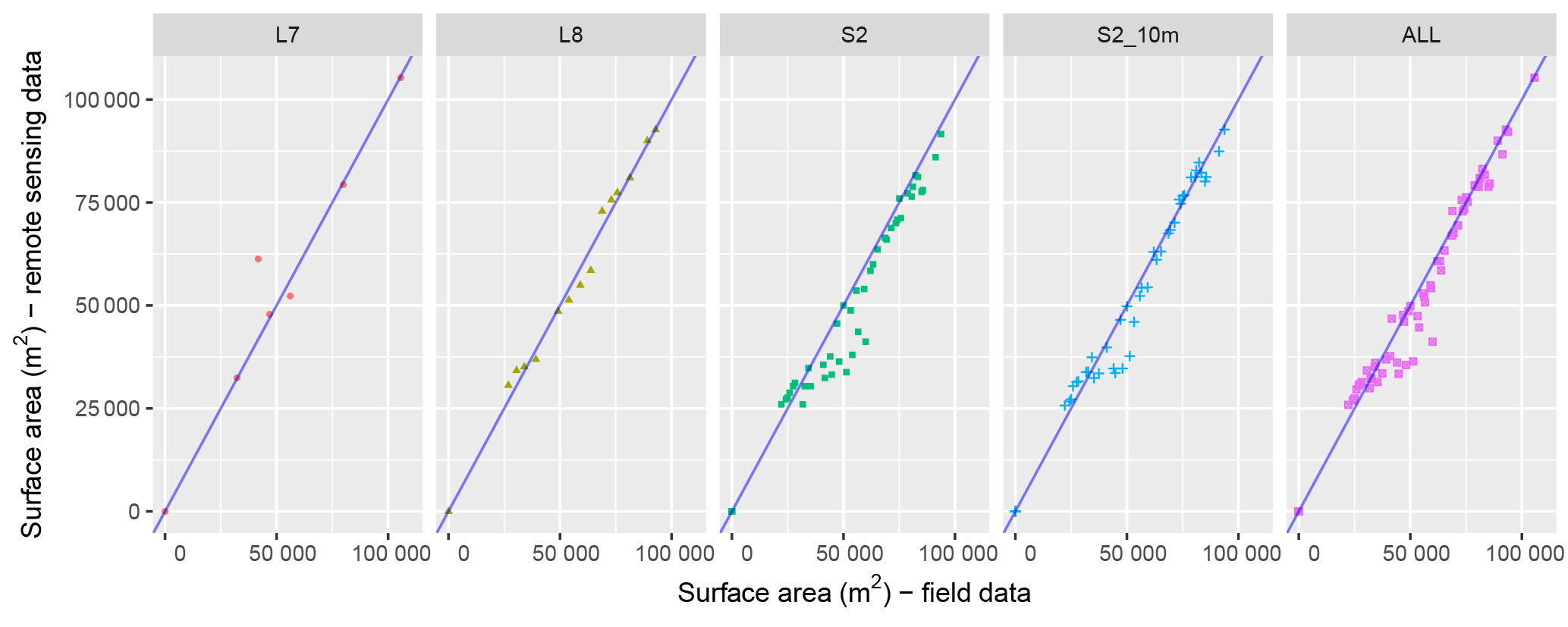
Figure 22Remotely sensed surface areas with Sentinel-2 and Landsat 7 and 8 data vs. field data over 2016–2017 on Lake Gouazine.
Validated against significant hydrometric field data, this paper demonstrates the potential and limitations of Landsat imagery to monitor surface water extent dynamics and water availability within the smallest reservoirs (1–10 ha). Results confirmed the superiority of the MNDWI out of six widely used band ratio indices to detect flooded areas in seven reservoirs of varying sizes and over three flood stages. Overall accuracy rates were high despite difficulties in shallow water and flooded vegetation and the MNDWI threshold remained sufficiently stable to allow automation across several lakes from 1 to 12 ha and over Landsat 5, 7, and 8 images. The performance of other water detection indices when used in semi-automation (fixed thresholds) reduced significantly due to their greater sensitivity to minor changes in thresholds. With the MNDWI, surface area errors remained low, under 15 % on five lakes, including the smallest ones, remarkable considering the demanding objective of detecting areas under 1 ha with 30 m spatial imagery.
Applied over 546 images, results highlight the impact of spatial inaccuracies as well as cloud and shadow interferences over small lakes. Residual errors from cloud uncertainties, due to undetected cirrus clouds and shadows, as well as greater vegetation, shallow water, and associated mixed pixels, led to a number of outliers which can be detrimental, notably on smaller lakes. Filtering images with excessive cloud and SLC presence reduced temporal resolution to 1.5 images month−1, which can lead to minor floods and those subject to high infiltration being overlooked by Landsat time series. With a mean RMSE of 9300 m2 and R2 reaching 0.9, the method however confirmed the operational potential of Landsat imagery to study surface water dynamics of floods over 3 ha, as well as long-term water availability (R2=0.82).
Comparisons with global water datasets (Pekel et al., 2016) notably confirmed the benefits and relevance of specific, complementary approaches for improving classification in smaller water bodies. Designed and calibrated to account for the specificities of small reservoirs, this semi-automated MNDWI approach reduced RMSE by 57 % in comparison, by minimizing omission errors from flooded vegetation and shallow waters. Accurate estimates of the total flooded surface area are notably important when converting lake surfaces to volumes (Busker et al., 2018) to quantify hydrological variables. Results also argue for the importance of exploiting all Landsat archive imagery to maximize temporal resolution, capture flood peaks, reproduce coherent flood dynamics, and improve water resource assessments considering the rapid flood declines in small lakes. Clearer distinction of clouds and SLC-off in the JRC datasets would have allowed finer filtering of images due to the non-systematic cloud error observed here. Continued research in improving cirrus cloud and shadow detection and notably specific methods capable of addressing the incremental change even on small land use objects remain essential (Zhu and Woodcock, 2014).
Results also provide evidence of the rising opportunities from remote sensing in small-scale hydrology, secured by the next generation of optical sensors providing free images every 5 days (Sentinel-2) with high spatial resolution (10–20 m). Greater spatial accuracy from 10 m pansharpened bands notably reduced RMSE by 12 % on the 2016–2017 floods compared to MNDWI on 20 m Sentinel-2 bands. Combining Landsat and Sentinel-2 imagery here reduced RMSE to 5200 m2 from 23 700 m2 on the 2016–2017 flood thanks to frequent observations and better detection of the flood peak. Monitoring flood dynamics with optical sensors remains however dependent on low cloud cover, and alternate optimization of clouds and SLC-off or concomitant imagery sources including active sensors (e.g. Sentinel-1) could also be used to maintain more observations at critical stages such as flood peaks (Eilander et al., 2014). Remotely sensed observations may also be combined with field data and modelling to overcome image availability issues and problems of incoherent hydrological dynamics.
Using free medium-resolution Landsat imagery, this method may be replicated regionally or globally to provide long-term datasets across small water bodies. Future research will help clarify whether the apparent stability of the MNDWI threshold across these seven lakes and in other regions (Ogilvie et al., 2015) allows the approach to be transposed without additional field calibration and whether automatic thresholding approaches may be complementary (Coltin et al., 2016; Vala and Baxi, 2013). Accurate long-term water availability assessments are notably required to inform farmers of water resources in the millions of small reservoirs worldwide (Lehner et al., 2011; Wisser et al., 2010) and to improve hydrological modelling. The spatialized information of the volumes captured by small lakes can be used to improve hydrological modelling in the lake catchments, especially runoff estimation due to poorly detected rainfall in semi-arid areas. Similarly, data assimilation techniques to combine the Landsat-derived flooded volumes can improve semi-distributed hydrological modelling of larger catchments. Reducing the uncertainties in the volumes captured by small lakes is essential to improve watershed management, e.g. to assess groundwater recharge from small lakes and to clarify the cumulative influence of these water conservation works in reducing downstream runoff.
Landsat L1T data are available from USGS Earth Explorer (USGS, 2018). Monthly water history rasters (Pekel et al., 2016) are available through Google Earth Engine (Gorelick, 2017), image collection ID JRC/GSW1_0/MonthlyHistory. Fmask is available at https://github.com/prs021/fmask. Details on the additional scripts and R packages used to process the Landsat imagery are provided in Appendix A. Sentinel-2 surface reflectance data are available for selected regions of the world from https://theia.cnes.fr.
The following preprocessing chain was applied to 596 Landsat images over 1999–2017. Functions belonging to the R rgdal, raster, sp, and landsat packages were used, but their code was adapted to account for the differences in Landsat 8 bands and metadata files.
A1 Radiometric normalization
Quantized calibrated (QCAL) digital numbers (DNs) for each pixel were converted to at-sensor (a.k.a. top-of-atmosphere, TOA) spectral radiance L by reversing the calibration process used by USGS (Chander et al., 2007). The linear transformation used (Eq. A1) can be rewritten as Eq. (A2) as DNmin is 0 and DNmax is 255. Grescale and Brescale are the “radiance multiplicative” and “radiance additive” rescaling factors, sometimes called gain and bias (or offset). These sensor- and band-specific factors were extracted automatically for each band and image from the Landsat metadata files.
where
A2 Atmospheric corrections
At-sensor radiance was then converted to at-canopy (at-surface) reflectance using the dark object subtraction (DOS) method (Chavez, 1996). The DOS approach encompasses conversion to at-sensor reflectance to account for intra-annual differences in Earth to Sun distance and solar illumination (Paolini et al., 2006). It also incorporates atmospheric corrections to estimate top-of-canopy (TOC) reflectance (Eq. A5) and account for the complex distorting effect of air molecules, aerosol particles, water vapour, carbon dioxide, methane, etc., which absorb and scatter electromagnetic waves (Hagolle et al., 2015). Absolute corrections were preferred over relative atmospheric correction methods such as pseudo invariant features (PIFs) and histogram matching as these do not account for the band specificity of atmospheric disturbances and are therefore not recommended with band ratio classifications (Lu et al., 2002). Furthermore, key inputs for physically based models of (part of the) atmospheric effects such as aerosol optical thickness were not available from nearby Aeronet sites for historical Landsat 5 and 7 data. DOS methods provide a simple, widely used method for atmospheric corrections, proven to perform well and as reliably as other algorithms and methods (Lu et al., 2002; Paolini et al., 2006; Song et al., 2001).
The DOS method supposes that certain objects within an image are dark (in complete shadow) and that radiance values measured for these objects are due to atmospheric scattering (path radiance, Lhaze) (Chavez, 1996). These dark objects are selected from the lowest DN value across at least 1000 pixels. This defines the starting haze value (SHV) which is converted from DN to TOA radiance according to Eq. (A2). As per Eq. (A8), an allowance is made considering that pixels are rarely completely dark and 1 % natural reflectance is subtracted. Lhaze converted to satellite reflectance is then subtracted to reflectance values across the image (Eq. A5). The improved DOS employed here calculates Lhaze for all bands using only one band (blue band) to “correlate haze values and maintain the spectral relationship between bands” (Chavez, 1996; Goslee, 2011). In the SWIR bands, where minimal scattering occurs, SHV is defined as 0 (Goslee, 2011).
Tauv is the atmospheric transmittance from the target to the sensor, Tauz is the atmospheric transmittance from the Sun to the target, and Edown is the downwelling diffuse spectral irradiance at the surface. The DOS1 level of correction which assumes no atmospheric transmission losses in either direction (Tauv and Tauz=1) and no diffuse downward radiation at the ground (Edown=0), i.e. corrects only for additive scattering, was used here. More complex corrections (for haze or aerosols) are less adapted to normalizing successive images as required here and do not improve overall accuracies (Goslee, 2011; Song et al., 2001).
Esun is the Earth to Sun distance in astronomical units (AUs) provided in the metadata files for OLI. For other sensors (ETM+, TM), this was calculated based on the date of acquisition indicated in the metadata (and function ESDIST in the R Landsat Goslee, 2011 package).
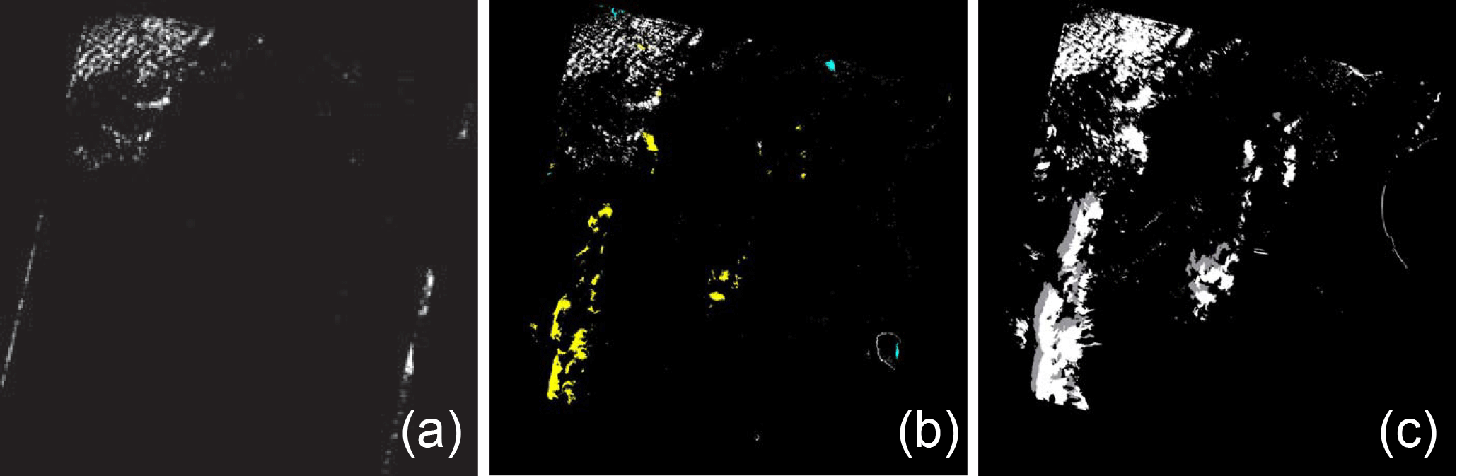
Figure A1Comparing cloud detection methods on the Landsat 8 29 March 2013 image: (a) clouds detected over 1.7 % of the image with the ACCA (Irish et al., 2006) and Goslee (2011) methods; (b) clouds including cirrus detected over 8.2 % of the image with the Landsat 8 1380 nm band; (c) clouds including cirrus and cloud shadows detected over 11.5 % of the image with the Fmask (Zhu and Woodcock, 2014) method.
sunelev is the solar elevation angle in degrees for the scene centre provided by the metadata file and again based on known changes in Earth–Sun geometry over the months. The complementary angle (90−sunelev) provides the local solar zenith angle.
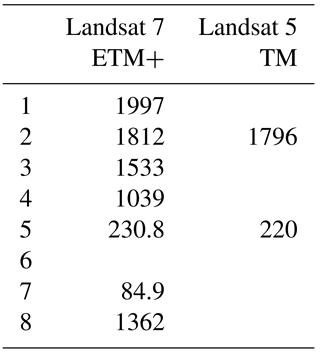
Exsun is the band-specific exoatmospheric solar irradiance constant in calculated based on Eq. (A9). For OLI, Lmax and REFmax are provided for each band. For ETM+ and TM sensors, Exsun for each band was taken from the literature (Table A1).
A3 Topographic normalization
Finally, topographic corrections to account for the effect on surface reflectance values of reduced illumination from inclined surfaces were implemented. The Minnaert algorithm (Minnaert, 1941), shown to perform as well as or better than C correction, cosine correction, and Gamma correction (Vanonckelen et al., 2013), was used. Minnaert adds a band-specific constant K to the cosine correction, a trigonometric correction defined in Eq. (A10) where ρt is the reflectance value generated by the inclined surface, and ρh is the value on a theoretical flat surface. Illumination is modelled as per Eq. (A11), where γi is the incident angle, slope angle is θp, solar zenith angle is θz, solar azimuth angle is ϕa, and aspect angle is ϕo. Slope and aspect were derived in R from the SRTM version 3 30 m digital elevation model, and information on solar azimuth and zenith angle were extracted from satellite and solar geometry in the metadata files.
Table A1Exoatmospheric solar constant per band for ETM+ and TM sensors (Chander et al., 2009).
A4 Cloud and shadow detection per lake
Fmask (Zhu and Woodcock, 2012), which uses top-of-atmosphere reflectances for all visible and IR bands, and brightness temperature for band 6 (Eq. A12) as inputs, was used to assess clouds and shadow presence on each image and over each lake cell. It reports a 96.41 % overall accuracy vs. 84.8 % for the Automated Cloud Cover Assessment (ACCA) algorithm (Irish et al., 2006) used originally by the USGS. DN values in Landsat thermal bands were converted to TOA radiance using Eq. (A2) and then to (brightness) temperature (Kelvin) using Eq. (A12).
K1 and K2 can be found in the Landsat 8 metadata and in the literature for Landsat 5 and 7 (Chander et al., 2009). ε is emissivity, and can be estimated as 0.95 to account for atmospheric interferences. The method then combines probability masks with a series of rule-based tests to identify potential cloud pixels based on the cloud spectral behaviour. Cloud shadows are modelled based upon estimating cloud height based on temperature, view angle, and solar illumination geometry reported in the metadata files (Huang et al., 2010; Zhu and Woodcock, 2012). In addition to cloud shadows, the Fmask version (3.2.1) used here also exploits the Landsat 8 1380 nm wavelength for the detection of the cirrus clouds (Fig. A1). This wavelength present on other lower spatial resolution sensors is strongly absorbed by the water vapour in the (lower) atmosphere; therefore, only high cirrus clouds where water vapour is low will reflect solar radiation in this wavelength. As discussed, associated methods combining the information from several (15 for Tmask) successive images to improve cloud shadow detection (Goodwin et al., 2013; Zhu and Woodcock, 2014) were not suitable, due to the localized and rapid changes investigated here.
AO conceived the research, carried out the analysis and wrote the article. GB, SM, MM and PLG helped design the approach and review the results and the article. RC, SM and AO contributed to field data acquisition.
The authors declare that they have no conflict of interest.
We gratefully acknowledge the collaboration from the Direction Générale
de l'Aménagement et de la Conservation des Terres Agricoles (DG ACTA) and
Direction Générale des Ressources en Eau (DGRE) in Tunis and local
representatives at the Kairouan and Siliana Commissariat Régional au
Développement Agricole (CRDA). These works were partly financed by the ANR
AMETHYST and SICMED DYSHYME projects. Sentinel-2 surface reflectance data
were obtained as part of the CNES THEIA Sentinel-2 project for Tunisia. SPOT
5 10 m imagery was provided through the CNES ISIS programme, request
703.
Edited by: Anas Ghadouani
Reviewed by: Manuela Grippa and C. Cudennec
Al Ali, Y., Touma, J., Zante, P., Nasri, S., and Albergel, J.: Water and sediment balances of a contour bench terracing system in a semi-arid cultivated zone (El Gouazine, central Tunisia), Hydrol. Sci. J., 53, 883–892, https://doi.org/10.1623/hysj.53.4.883, 2008. a
Albergel, J. and Rejeb, N.: Les lacs collinaires en Tunisie: Enjeux, Contraintes et Perspectives, C. R. Acad. Agric. Fr., 83, 77–88, 1997. a, b, c
Albergel, J., Pepin, Y., Nasri, S., and Boufaroua, M.: Erosion et transport solide dans des petits bassins versants méditerranéens, IAHS-AISH P., 278, 373–379, 2003. a
Alsdorf, D., Bates, P., and Melack, J.: Spatial and temporal complexity of the Amazon flood measured from space, Geophys. Res. Lett., 34, L08402, https://doi.org/10.1029/2007GL029447, 2007. a
Annor, F. O., van de Giesen, N., Liebe, J., van de Zaag, P., Tilmant, A., and Odai, S.: Delineation of small reservoirs using radar imagery in a semi-arid environment: A case study in the upper east region of Ghana, Phys. Chem. Earth Pt. A/B/C, 34, 309–315, https://doi.org/10.1016/j.pce.2008.08.005, 2009. a, b, c, d, e
Avisse, N., Tilmant, A., Müller, M. F., and Zhang, H.: Monitoring small reservoirs' storage with satellite remote sensing in inaccessible areas, Hydrol. Earth Syst. Sci., 21, 6445–6459, https://doi.org/10.5194/hess-21-6445-2017, 2017. a, b, c, d
Baup, F., Frappart, F., and Maubant, J.: Combining high-resolution satellite images and altimetry to estimate the volume of small lakes, Hydrol. Earth Syst. Sci., 18, 2007–2020, https://doi.org/10.5194/hess-18-2007-2014, 2014. a, b, c
Bédard, F., Reichert, G., Dobbins, R., and Trépanier, I.: Evaluation of segment-based gap-filled Landsat ETM+ SLC-off satellite data for land cover classification in southern Saskatchewan, Canada, Int. J. Remote Sens., 29, 2041–2054, https://doi.org/10.1080/01431160701281064, 2008. a
Bergé-Nguyen, M. and Crétaux, J.-F.: Inundations in the Inner Niger Delta: Monitoring and Analysis Using MODIS and Global Precipitation Datasets, Remote Sens., 7, 2127–2151, https://doi.org/10.3390/rs70202127, 2015. a
Bouma, J. A., Biggs, T. W., and Bouwer, L. M.: The downstream externalities of harvesting rainwater in semi-arid watersheds: An Indian case study, Agr. Water Manage., 98, 1162–1170, https://doi.org/10.1016/j.agwat.2011.02.010, 2011. a
Burte, J., Coudrain, A., Frischkorn, H., Chaffaut, I., and Kosuth, P.: Impacts anthropiques sur les termes du bilan hydrologique d'un aquifère alluvial dans le Nordeste semi-aride, Brésil, Hydrol. Sci. J., 50, 95–110, https://doi.org/10.1623/hysj.50.1.95.56337, 2005. a
Busker, T., de Roo, A., Gelati, E., Schwatke, C., Adamovic, M., Bisselink, B., Pekel, J.-F., and Cottam, A.: A global lake and reservoir volume analysis using a surface water dataset and satellite altimetry, Hydrol. Earth Syst. Sci. Discuss., https://doi.org/10.5194/hess-2018-21, in review, 2018. a, b
Carper, W. J., Lillesand, T. M., and Kiefer, R. W.: The use of intensity-hue-saturation transformations for merging SPOT panchromatic and multispectral image data, Photogramm. Eng. Rem. S., 56, 459–467, 1990. a
Chander, G., Markham, B. L., and Barsi, J. A.: Revised landsat-5 thematic mapper radiometric calibration, IEEE Geosci. Remote S., 4, 490–494, https://doi.org/10.1109/LGRS.2007.898285, 2007. a
Chander, G., Markham, B. L., and Helder, D. L.: Summary of current radiometric calibration coefficients for Landsat MSS, TM, ETM+, and EO-1 ALI sensors, Remote Sens. Environ., 113, 893–903, https://doi.org/10.1016/j.rse.2009.01.007, 2009. a, b
Chavez, P. S. J.: Image-based atmospheric corrections- revisited and improved, Photogramm. Eng. Rem. S., 62, 1025–1035, https://doi.org/0099-1112/96/6209-1025, 1996. a, b, c
Chen, J., Zhu, X., Vogelmann, J. E., Gao, F., and Jin, S.: A simple and effective method for filling gaps in Landsat ETM+ SLC-off images, Remote Sens. Environ., 115, 1053–1064, https://doi.org/10.1016/j.rse.2010.12.010, 2011. a
CNEA: Etude d'impact des travaux de conservation des eaux et du sol dans le gouvernorat de Kairouan, Tech. rep., Centre National des Etudes Agricoles (CNEA), Tunisie, 2006. a
Collinet, J. and Zante, P.: Analyse du ravinement de bassins versants à retenues collinaires sur sols à fortes dynamiques structurales (Tunisie), Geomorphologie, 11, 61–74, https://doi.org/10.4000/geomorphologie.257, 2005. a
Coltin, B., McMichael, S., Smith, T., and Fong, T.: Automatic boosted flood mapping from satellite data, Int. J. Remote Sens., 37, 993–1015, https://doi.org/10.1080/01431161.2016.1145366, 2016. a
Crétaux, J.-F., Abarca-del Río, R., Bergé-Nguyen, M., Arsen, A., Drolon, V., Clos, G., and Maisongrande, P.: Lake Volume Monitoring from Space, Surv. Geophys., 37, 269–305, https://doi.org/10.1007/s10712-016-9362-6, 2016. a, b
Cudennec, C., Slimani, M., and Le Goulven, P.: Accounting for sparsely observed rainfall space-time variability in a rainfall-runoff model of a semiarid Tunisian basin, Hydrol. Sci. J., 50, 617–630, https://doi.org/10.1623/hysj.2005.50.4.617, 2005. a
Doxani, G., Vermote, E., Roger, J.-C., Gascon, F., Adriaensen, S., Frantz, D., Hagolle, O., Hollstein, A., Kirches, G., Li, F., Louis, J., Mangin, A., Pahlevan, N., Pflug, B., and Vanhellemont, Q.: Atmospheric Correction Inter-Comparison Exercise, Remote Sens., 10, 352, https://doi.org/10.3390/rs10020352, 2018. a
Du, Y., Zhang, Y., Ling, F., Wang, Q., Li, W., and Li, X.: Water Bodies' Mapping from Sentinel-2 Imagery with Modified Normalized Difference Water Index at 10 m Spatial Resolution Produced by Sharpening the SWIR Band, Remote Sens., 8, 354, https://doi.org/10.3390/rs8040354, 2016. a, b
Eilander, D., Annor, F., Iannini, L., and van de Giesen, N.: Remotely Sensed Monitoring of Small Reservoir Dynamics: A Bayesian Approach, Remote Sens., 6, 1191–1210, https://doi.org/10.3390/rs6021191, 2014. a
Feng, M., Sexton, J. O., Channan, S., and Townshend, J. R.: A global, high-resolution (30-m) inland water body dataset for 2000: first results of a topographic-spectral classification algorithm, Int. J. Digit. Earth, 9, 113–133, https://doi.org/10.1080/17538947.2015.1026420, 2016. a, b
Feyisa, G. L., Meilby, H., Fensholt, R., and Proud, S. R.: Automated Water Extraction Index: A new technique for surface water mapping using Landsat imagery, Remote Sens. Environ., 140, 23–35, https://doi.org/10.1016/j.rse.2013.08.029, 2014. a, b, c, d, e
Fisher, A. and Danaher, T.: A water index for SPOT5 HRG satellite imagery, New South Wales, Australia, determined by linear discriminant analysis, Remote Sens., 5, 5907–5925, https://doi.org/10.3390/rs5115907, 2013. a
Foga, S., Scaramuzza, P. L., Guo, S., Zhu, Z., Dilley, R. D., Beckmann, T., Schmidt, G. L., Dwyer, J. L., Joseph Hughes, M., and Laue, B.: Cloud detection algorithm comparison and validation for operational Landsat data products, Remote Sens. Environ., 194, 379–390, https://doi.org/10.1016/J.RSE.2017.03.026, 2017. a
Gao, B.-C.: NDWI – A normalized difference water index for remote sensing of vegetation liquid water from space, Remote Sens. Environ., 58, 257–266, https://doi.org/10.1016/S0034-4257(96)00067-3, 1996. a, b
Gardelle, J., Hiernaux, P., Kergoat, L., and Grippa, M.: Less rain, more water in ponds: a remote sensing study of the dynamics of surface waters from 1950 to present in pastoral Sahel (Gourma region, Mali), Hydrol. Earth Syst. Sci., 14, 309–324, https://doi.org/10.5194/hess-14-309-2010, 2010. a
Gay, D.: Fonctionnement et bilan de retenues artificielles en Tunisie: approche hydrochimique et isotopique, PhD thesis, Université Paris XI, France, 2004. a
Goodwin, N. R., Collett, L. J., Denham, R. J., Flood, N., and Tindall, D.: Cloud and cloud shadow screening across Queensland, Australia: An automated method for Landsat TM/ETM+ time series, Remote Sens. Environ., 134, 50–65, https://doi.org/10.1016/j.rse.2013.02.019, 2013. a
Gorelick, N., Hancher, M., Dixon, M., Ilyushchenko, S., Thau, D., and Moore, R.: Google Earth Engine: Planetary-scale geospatial analysis for everyone, Remote Sens. Environ., 202, 18–27, https://doi.org/10.1016/j.rse.2017.06.031, 2017.
Goslee, S. C.: Analyzing Remote Sensing Data in R: The landsat Package, J. Stat. Softw., 43, 1–25, https://doi.org/10.18637/jss.v043.i04, 2011. a, b, c, d, e
Grunberger, O., Montoroi, J., and Nasri, S.: Quantification of water exchange between a hill reservoir and groundwater using hydrological and isotopic modelling (El Gouazine, Tunisia), C. R. Geosci., 336, 1453–1462, https://doi.org/10.1016/j.crte.2004.08.006, 2004. a, b
Gumbricht, T., Wolski, P., Frost, P., and McCarthy, T.: Forecasting the spatial extent of the annual flood in the Okavango Delta, Botswana, J. Hydrol., 290, 178–191, https://doi.org/10.1016/j.jhydrol.2003.11.010, 2004. a
Guo, M., Li, J., Sheng, C., Xu, J., and Wu, L.: A Review of Wetland Remote Sensing, Sensors, 17, 777, https://doi.org/10.3390/s17040777, 2017. a
Habi, M. and Morsli, B.: Contraintes et perspectives des retenues collinaires dans le Nord-Ouest algérien, Sécheresse, 22, 49–56, https://doi.org/10.1684/sec.2011.0293, 2011. a
Hagolle, O., Huc, M., Pascual, D., and Dedieu, G.: A Multi-Temporal and Multi-Spectral Method to Estimate Aerosol Optical Thickness over Land, for the Atmospheric Correction of FormoSat-2, LandSat, VENS and Sentinel-2 Images, Remote Sens., 7, 2668–2691, https://doi.org/10.3390/rs70302668, 2015. a, b
Hentati, A., Kawamura, A., Amaguchi, H., and Iseri, Y.: Evaluation of sedimentation vulnerability at small hillside reservoirs in the semi-arid region of Tunisia using the Self-Organizing Map, Geomorphology, 122, 56–64, https://doi.org/10.1016/j.geomorph.2010.05.013, 2010. a, b
Huang, C., Thomas, N., Goward, S. N., Masek, J. G., Zhu, Z., Townshend, J. R. G., and Vogelmann, J. E.: Automated masking of cloud and cloud shadow for forest change analysis using Landsat images, Int. J. Remote Sens., 31, 5449–5464, https://doi.org/10.1080/01431160903369642, 2010. a
Irish, R. R., Barker, J. L., Goward, S. N., and Arvidson, T.: Characterization of the Landsat-7 ETM+ Automated Cloud-Cover Assessment (ACCA) Algorithm, Photogramm. Eng. Rem. S., 72, 1179–1188, https://doi.org/10.14358/PERS.72.10.1179, 2006. a, b
Jain, A. K.: Data clustering: 50 years beyond K-means, Pattern Recogn. Lett., 31, 651–666, https://doi.org/10.1016/j.patrec.2009.09.011, 2010. a, b, c
Ji, L., Zhang, L., and Wylie, B.: Analysis of Dynamic Thresholds for the Normalized Difference Water Index, Photogramm. Eng. Rem. S., 75, 1307–1317, https://doi.org/10.14358/PERS.75.11.1307, 2009. a, b, c
Ji, L., Geng, X., Sun, K., Zhao, Y., and Gong, P.: Target Detection Method for Water Mapping Using Landsat 8 OLI/TIRS Imagery, Water, 7, 794–817, https://doi.org/10.3390/w7020794, 2015. a
Jiang, H., Feng, M., Zhu, Y., Lu, N., Huang, J., and Xiao, T.: An Automated Method for Extracting Rivers and Lakes from Landsat Imagery, Remote Sens., 6, 5067–5089, https://doi.org/10.3390/rs6065067, 2014. a, b
Jones, S., Fremier, A., DeClerck, F., Smedley, D., Ortega Pieck, A., and Mulligan, M.: Big Data and Multiple Methods for Mapping Small Reservoirs: Comparing Accuracies for Applications in Agricultural Landscapes, Remote Sens., 9, 1307, https://doi.org/10.3390/rs9121307, 2017. a, b
Kaplan, G. and Avdan, U.: Sentinel-2 Pan Sharpening – Comparative Analysis, Proceedings, 2, 345, https://doi.org/10.3390/ecrs-2-05158, 2018. a
Kingumbi, A.: Modélisation hydrologique d'un bassin affecté par des changements d'occupation. Cas du Merguellil en Tunisie Centrale, PhD thesis, Université de Tunis El Manar, Ecole Nationale d'Ingénieurs de Tunis, Tunisia, 2006. a
Kingumbi, A., Bargaoui, Z., Ledoux, E., Besbes, M., and Hubert, P.: Modélisation hydrologique stochastique d'un bassin affecté par des changements d'occupation: cas du Merguellil en Tunisie centrale, Hydrol. Sci. J., 52, 1232–1252, https://doi.org/10.1623/hysj.52.6.1232, 2007. a
Klein, I., Dietz, A., Gessner, U., Dech, S., and Kuenzer, C.: Results of the Global WaterPack: a novel product to assess inland water body dynamics on a daily basis, Remote Sens. Lett., 6, 78–87, https://doi.org/10.1080/2150704X.2014.1002945, 2015. a
Kuenzer, C., Klein, I., Ullmann, T., Georgiou, E., Baumhauer, R., and Dech, S.: Remote Sensing of River Delta Inundation: Exploiting the Potential of Coarse Spatial Resolution, Temporally-Dense MODIS Time Series, Remote Sens., 7, 8516–8542, https://doi.org/10.3390/rs70708516, 2015. a
Lacaux, J., Tourre, Y., Vignolles, C., Ndione, J., and Lafaye, M.: Classification of ponds from high-spatial resolution remote sensing: Application to Rift Valley Fever epidemics in Senegal, Remote Sens. Environ., 106, 66–74, https://doi.org/10.1016/j.rse.2006.07.012, 2007. a, b, c
Lacombe, G.: Evolution et usages de la ressource en eau dans un bassin versant amenagé semi-aride, Le cas du Merguellil en Tunisie Centrale, PhD thesis, Université Montpellier II, France, 2007. a, b, c, d, e, f
Leauthaud, C., Belaud, G., Duvail, S., Moussa, R., Grünberger, O., and Albergel, J.: Characterizing floods in the poorly gauged wetlands of the Tana River Delta, Kenya, using a water balance model and satellite data, Hydrol. Earth Syst. Sci., 17, 3059–3075, https://doi.org/10.5194/hess-17-3059-2013, 2013. a
Leduc, C., Ben Ammar, S., Favreau, G., Beji, R., Virrion, R., Lacombe, G., Tarhouni, J., Aouadi, C., Zenati Chelli, B., Jebnoun, N., Oi, M., Michelot, J., and Zouari, K.: Impacts of hydrological changes in the Mediterranean zone: environmental modifications and rural development in the Merguellil catchment, central Tunisia, Hydrol. Sci. J., 52, 1162–1178, https://doi.org/10.1623/hysj.52.6.1162, 2007. a
Lehner, B., Liermann, C. R., Revenga, C., Vörösmarty, C., Fekete, B., Crouzet, P., Döll, P., Endejan, M., Frenken, K., Magome, J., Nilsson, C., Robertson, J. C., Rödel, R., Sindorf, N., and Wisser, D.: High-resolution mapping of the world's reservoirs and dams for sustainable river-flow management, Front. Ecol. Environ., 9, 494–502, https://doi.org/10.1890/100125, 2011. a
Li, Q. and Gowing, J.: A Daily Water Balance Modelling Approach for Simulating Performance of Tank-Based Irrigation Systems, Water Resour. Manag., 19, 211–231, https://doi.org/10.1007/s11269-005-2702-9, 2005. a, b
Liebe, J., van de Giesen, N., and Andreini, M.: Estimation of small reservoir storage capacities in a semi-arid environment, Phys. Chem. Earth Pt. A/B/C, 30, 448–454, https://doi.org/10.1016/j.pce.2005.06.011, 2005. a, b, c, d, e, f
Lu, D., Mausel, P., Brondizio, E., and Moran, E.: Assessment of atmospheric correction methods for Landsat TM data applicable to Amazon basin LBA research, Int. J. Remote Sens., 23, 2651–2671, https://doi.org/10.1080/01431160110109642, 2002. a, b
Ma, M., Wang, X., Veroustraete, F., and Dong, L.: Change in area of Ebinur Lake during the 1998–2005 period, Int. J. Remote Sens., 28, 5523–5533, https://doi.org/10.1080/01431160601009698, 2007. a, b
Mahé, G., Orange, D., Mariko, A., and Bricquet, J. P.: Estimation of the flooded area of the Inner Delta of the River Niger in Mali by hydrological balance and satellite data, IAHS-AISH P., 344, 138–143, 2011. a
Martinez, J.-M. and Le Toan, T.: Mapping of flood dynamics and spatial distribution of vegetation in the Amazon floodplain using multitemporal SAR data, Remote Sens. Environ., 108, 209–223, https://doi.org/10.1016/j.rse.2006.11.012, 2007. a
Massuel, S., Perrin, J., Mascre, C., Mohamed, W., Boisson, A., and Ahmed, S.: Managed aquifer recharge in South India: What to expect from small percolation tanks in hard rock?, J. Hydrol., 512, 157–167, https://doi.org/10.1016/j.jhydrol.2014.02.062, 2014. a
Maxwell, S.: Filling Landsat ETM+ SLC-off Gaps Using a Segmentation Model Approach, Photogramm. Eng. Rem. S., 70, 1109–1111, 2004. a, b
McFeeters, S. K.: The use of the Normalized Difference Water Index (NDWI) in the delineation of open water features, Int. J. Remote Sens., 17, 1425–1432, https://doi.org/10.1080/01431169608948714, 1996. a, b
Mialhe, F., Gunnell, Y., and Mering, C.: Synoptic assessment of water resource variability in reservoirs by remote sensing: General approach and application to the runoff harvesting systems of south India, Water Resour. Res., 44, W05411, https://doi.org/10.1029/2007WR006065, 2008. a, b, c
Minnaert, M.: The reciprocity principle in lunar photometry, Astrophys. J., 93, 403–410, https://doi.org/10.1086/144279, 1941. a
Mohamed, Y., Bastiaanssen, W. G. M., and Savenije, H. H. G.: Spatial variability of evaporation and moisture storage in the swamps of the upper Nile studied by remote sensing techniques, J. Hydrol., 289, 145–164, https://doi.org/10.1016/j.jhydrol.2003.11.038, 2004. a
Mueller, N., Lewis, A., Roberts, D., Ring, S., Melrose, R., Sixsmith, J., Lymburner, L., McIntyre, A., Tan, P., Curnow, S., and Ip, A.: Water observations from space: Mapping surface water from 25 years of Landsat imagery across Australia, Remote Sens. Environ., 174, 341–352, https://doi.org/10.1016/j.rse.2015.11.003, 2016. a, b, c, d, e
Nasri, S., Cudennec, C., Albergel, J., and Berndtsson, R.: Use of a geomorphological transfer function to model design floods in small hillside catchments in semiarid Tunisia, J. Hydrol., 287, 197–213, https://doi.org/10.1016/j.jhydrol.2003.10.001, 2004. a
Nyssen, J., Clymans, W., Descheemaeker, K., Poesen, J., Vandecasteele, I., Vanmaercke, M., Zenebe, A., Van Camp, M., Haile, M., Haregeweyn, N., Moeyersons, J., Martens, K., Gebreyohannes, T., Deckers, J., and Walraevens, K.: Impact of soil and water conservation measures on catchment hydrological response-a case in north Ethiopia, Hydrol. Process., 24, 1880–1895, https://doi.org/10.1002/hyp.7628, 2010. a, b
Ogilvie, A.: Upscaling water availability and water use assessments in hydro-sociosystems: the small reservoirs of the Merguellil catchment (Central Tunisia), PhD thesis, Université de Montpellier, France and King's College London, UK, 2015. a, b
Ogilvie, A., Belaud, G., Delenne, C., Bailly, J.-S., Bader, J.-C., Oleksiak, A., Ferry, L., and Martin, D.: Decadal monitoring of the Niger Inner Delta flood dynamics using MODIS optical data, J. Hydrol., 523, 368–383, https://doi.org/10.1016/j.jhydrol.2015.01.036, 2015. a, b, c, d, e, f
Ogilvie, A., Belaud, G., Massuel, S., Mulligan, M., Le Goulven, P., and Calvez, R.: Assessing Floods and Droughts in Ungauged Small Reservoirs with Long-Term Landsat Imagery, Geosciences, 6, 42, https://doi.org/10.3390/GEOSCIENCES6040042, 2016a. a, b, c
Ogilvie, A., Le Goulven, P., Leduc, C., Calvez, R., and Mulligan, M.: Réponse hydrologique d'un bassin semi-aride aux événements pluviométriques et aménagements de versant (bassin du Merguellil, Tunisie centrale), Hydrol. Sci. J., 61, 441–453, https://doi.org/10.1080/02626667.2014.934249, 2016b. a, b
Ouma, Y. O. and Tateishi, R.: A water index for rapid mapping of shoreline changes of five East African Rift Valley lakes: an empirical analysis using Landsat TM and ETM+ data, Int. J. Remote Sens., 27, 3153–3181, https://doi.org/10.1080/01431160500309934, 2006. a, b
Palmer, S. C. J., Kutser, T., and Hunter, P. D.: Remote sensing of inland waters: Challenges, progress and future directions, Remote Sens. Environ., 157, 1–8, https://doi.org/10.1016/j.rse.2014.09.021, 2015. a
Paolini, L., Grings, F., Sobrino, J. A., Jiménez Muñoz, J. C., and Karszenbaum, H.: Radiometric correction effects in Landsat multi-date/multi-sensor change detection studies, Int. J. Remote Sens., 27, 685–704, https://doi.org/10.1080/01431160500183057, 2006. a, b
Papa, F., Prigent, C., Aires, F., Jimenez, C., Rossow, W. B., and Matthews, E.: Interannual variability of surface water extent at the global scale, 1993–2004, J. Geophys. Res., 115, D12111, https://doi.org/10.1029/2009JD012674, 2010. a
Pekel, J.-F., Cottam, A., Gorelick, N., and Belward, A. S.: High-resolution mapping of global surface water and its long-term changes, Nature, 540, 418–422, https://doi.org/10.1038/nature20584, 2016. a, b, c, d, e, f, g, h, i, j, k, l, m, n, o, p, q, r, s, t
Prigent, C., Papa, F., Aires, F., Rossow, W. B., and Matthews, E.: Global inundation dynamics inferred from multiple satellite observations, 1993–2000, J. Geophys. Res., 112, D12107, https://doi.org/10.1029/2006JD007847, 2007. a
Qi, S., Brown, D. G., Tian, Q., Jiang, L., Zhao, T., and Bergen, K. M.: Inundation Extent and Flood Frequency Mapping Using LANDSAT Imagery and Digital Elevation Models, GIsci. Remote Sens., 46, 101–127, https://doi.org/10.2747/1548-1603.46.1.101, 2009. a
Ran, L. and Lu, X. X.: Delineation of reservoirs using remote sensing and their storage estimate: an example of the Yellow River basin, China, Hydrol. Process., 26, 1215–1229, https://doi.org/10.1002/hyp.8224, 2012. a
Rodrigues, L. N., Sano, E. E., Steenhuis, T. S., and Passo, D. P.: Estimation of Small Reservoir Storage Capacities with Remote Sensing in the Brazilian Savannah Region, Water Resour. Manag., 26, 873–882, https://doi.org/10.1007/s11269-011-9941-8, 2011. a
Rouse, J., Haas, J., Schell, J., and Deering, D.: Monitoring vegetation systems in the Great Plains with ERTS, in: Proceedings 3rd ERTS Symposium, NASA SP353, 309–317, Washington DC, USA, 1973. a, b
Sakamoto, T., Van Nguyen, N., Kotera, A., Ohno, H., Ishitsuka, N., and Yokozawa, M.: Detecting temporal changes in the extent of annual flooding within the Cambodia and the Vietnamese Mekong Delta from MODIS time-series imagery, Remote Sens. Environ., 109, 295–313, https://doi.org/10.1016/j.rse.2007.01.011, 2007. a
Sawunyama, T., Senzanje, A., and Mhizha, A.: Estimation of small reservoir storage capacities in Limpopo River Basin using geographical information systems (GIS) and remotely sensed surface areas: Case of Mzingwane catchment, Phys. Chem. Earth Pt. A/B/C, 31, 935–943, https://doi.org/10.1016/j.pce.2006.08.008, 2006. a, b, c, d, e, f, g
Scaramuzza, P., Micijevic, E., and Chander, G.: SLC gap-filled products phase one methodology, Landsat Technical Notes, available at: https://landsat.usgs.gov/documents/SLC_Gap_Fill_Methodology.pdf (last access: 10 August 2018), 2004. a
Schwatke, C., Dettmering, D., Bosch, W., and Seitz, F.: DAHITI – an innovative approach for estimating water level time series over inland waters using multi-mission satellite altimetry, Hydrol. Earth Syst. Sci., 19, 4345–4364, https://doi.org/10.5194/hess-19-4345-2015, 2015. a
Seiler, R., Schmidt, J., Diallo, O., and Csaplovics, E.: Flood monitoring in a semi-arid environment using spatially high resolution radar and optical data, J. Environ. Manage., 90, 2121–2129, https://doi.org/10.1016/j.jenvman.2007.07.035, 2009. a
Solander, K. C., Reager, J. T., and Famiglietti, J. S.: How well will the Surface Water and Ocean Topography (SWOT) mission observe global reservoirs?, Water Resour. Res., 52, 2123–2140, https://doi.org/10.1002/2015WR017952, 2016. a
Song, C., Woodcock, C. E., Seto, K. C., Lenney, M. P., and Macomber, S. A.: Classification and Change Detection Using Landsat TM Data, Remote Sens. Environ., 75, 230–244, https://doi.org/10.1016/S0034-4257(00)00169-3, 2001. a, b
Soti, V., Puech, C., Lo Seen, D., Bertran, A., Vignolles, C., Mondet, B., Dessay, N., and Tran, A.: The potential for remote sensing and hydrologic modelling to assess the spatio-temporal dynamics of ponds in the Ferlo Region (Senegal), Hydrol. Earth Syst. Sci., 14, 1449–1464, https://doi.org/10.5194/hess-14-1449-2010, 2010. a
Sun, W., Du, B., and Xiong, S.: Quantifying Sub-Pixel Surface Water Coverage in Urban Environments Using Low-Albedo Fraction from Landsat Imagery, Remote Sens., 9, 428, https://doi.org/10.3390/rs9050428, 2017. a
Swenson, S. and Wahr, J.: Monitoring the water balance of Lake Victoria, East Africa, from space, J. Hydrol., 370, 163–176, https://doi.org/10.1016/j.jhydrol.2009.03.008, 2009. a
Talineau, J., Selmi, S., and Alaya, K.: Lacs collinaires en Tunisie semi-aride, Sécheresse, 5, 251–256, 1994. a
Tulbure, M. G., Broich, M., Stehman, S. V., and Kommareddy, A.: Surface water extent dynamics from three decades of seasonally continuous Landsat time series at subcontinental scale in a semi-arid region, Remote Sens. Environ., 178, 142–157, https://doi.org/10.1016/j.rse.2016.02.034, 2016. a
USGS: Earth Resources Observation and Science (EROS) Center, Landsat Collection 1 Level 1, available at: https://earthexplorer.usgs.gov, last access: 11 August 2018
Vala, H. J. and Baxi, A.: A review on Otsu image segmentation algorithm, International Journal of Advanced Research in Computer Engineering and Technology, 2, 387–389, 2013. a
Van Der Meer, F.: Spectral unmixing of Landsat Thematic Mapper data, Int. J. Remote Sens., 16, 3189–3194, https://doi.org/10.1080/01431169508954622, 1995. a
Vanonckelen, S., Lhermitte, S., and Van Rompaey, A.: The effect of atmospheric and topographic correction methods on land cover classification accuracy, Int. J. Appl. Earth Obs. Geoinf., 24, 9–21, https://doi.org/10.1016/j.jag.2013.02.003, 2013. a
Venot, J. P. and Krishnan, J.: Discursive framing: Debates over small reservoirs in the Rural South, Water Altern., 4, 316–324, 2011. a
Vermote, E., Justice, C., Claverie, M., and Franch, B.: Preliminary analysis of the performance of the Landsat 8/OLI land surface reflectance product, Remote Sens. Environ., 185, 46–56, https://doi.org/10.1016/J.RSE.2016.04.008, 2016. a
Verpoorter, C., Kutser, T., Seekell, D. A., and Tranvik, L. J.: A Global Inventory of Lakes Based on High-Resolution Satellite Imagery, Geophys. Res. Lett., 41, 6396–6402, https://doi.org/10.1002/2014GL060641, 2014. a
Vogelmann, J. E., Helder, D., Morfitt, R., Choate, M. J., Merchant, J. W., and Bulley, H.: Effects of Landsat 5 Thematic Mapper and Landsat 7 Enhanced Thematic Mapper plus radiometric and geometric calibrations and corrections on landscape characterization, Remote Sens. Environ., 78, 55–70, https://doi.org/10.1016/S0034-4257(01)00249-8, 2001. a
Wisser, D., Frolking, S., Douglas, E. M., Fekete, B. M., Schumann, A. H., and Vörösmarty, C. J.: The significance of local water resources captured in small reservoirs for crop production – A global-scale analysis, J. Hydrol., 384, 264–275, https://doi.org/10.1016/j.jhydrol.2009.07.032, 2010. a, b
Wolski, P. and Murray-Hudson, M.: An investigation of permanent and transient changes in flood distribution and outflows in the Okavango Delta, Botswana, Phys. Chem. Earth Pt. A/B/C, 33, 157–164, https://doi.org/10.1016/j.pce.2007.04.008, 2008. a
Xu, H.: Modification of normalised difference water index (NDWI) to enhance open water features in remotely sensed imagery, Int. J. Remote Sens., 27, 3025–3033, https://doi.org/10.1080/01431160600589179, 2006. a, b, c
Yamazaki, D. and Trigg, M. A.: Hydrology: The dynamics of Earth's surface water, Nature, 540, 348–349, https://doi.org/10.1038/nature21100, 2016. a, b
Yamazaki, D., Trigg, M. A., and Ikeshima, D.: Development of a global ∼90 m water body map using multi-temporal Landsat images, Remote Sens. Environ., 171, 337–351, https://doi.org/10.1016/j.rse.2015.10.014, 2015. a, b, c, d
Yin, G., Mariethoz, G., and McCabe, M.: Gap-Filling of Landsat 7 Imagery Using the Direct Sampling Method, Remote Sens., 9, 12, https://doi.org/10.3390/rs9010012, 2016. a
Zeng, C., Shen, H., and Zhang, L.: Recovering missing pixels for Landsat ETM+ SLC-off imagery using multi-temporal regression analysis and a regularization method, Remote Sens. Environ., 131, 182–194, https://doi.org/10.1016/j.rse.2012.12.012, 2013. a, b, c, d, e
Zhu, Z. and Woodcock, C. E.: Object-based cloud and cloud shadow detection in Landsat imagery, Remote Sens. Environ., 118, 83–94, https://doi.org/10.1016/j.rse.2011.10.028, 2012. a, b, c, d
Zhu, Z. and Woodcock, C. E.: Automated cloud, cloud shadow, and snow detection in multitemporal Landsat data: An algorithm designed specifically for monitoring land cover change, Remote Sens. Environ., 152, 217–234, https://doi.org/10.1016/j.rse.2014.06.012, 2014. a, b, c, d, e, f