the Creative Commons Attribution 4.0 License.
the Creative Commons Attribution 4.0 License.
 | 13 Sep 2018
Spatial prediction of groundwater spring potential mapping based on an adaptive neuro-fuzzy inference system and metaheuristic optimization
Khabat Khosravi
Dieu Tien Bui
Groundwater is one of the most valuable natural resources in the world (Jha et al., 2007). However, it is not an unlimited resource; therefore understanding groundwater potential is crucial to ensure its sustainable use. The aim of the current study is to propose and verify new artificial intelligence methods for the spatial prediction of groundwater spring potential mapping at the Koohdasht–Nourabad plain, Lorestan province, Iran. These methods are new hybrids of an adaptive neuro-fuzzy inference system (ANFIS) and five metaheuristic algorithms, namely invasive weed optimization (IWO), differential evolution (DE), firefly algorithm (FA), particle swarm optimization (PSO), and the bees algorithm (BA). A total of 2463 spring locations were identified and collected, and then divided randomly into two subsets: 70 % (1725 locations) were used for training models and the remaining 30 % (738 spring locations) were utilized for evaluating the models. A total of 13 groundwater conditioning factors were prepared for modeling, namely the slope degree, slope aspect, altitude, plan curvature, stream power index (SPI), topographic wetness index (TWI), terrain roughness index (TRI), distance from fault, distance from river, land use/land cover, rainfall, soil order, and lithology. In the next step, the step-wise assessment ratio analysis (SWARA) method was applied to quantify the degree of relevance of these groundwater conditioning factors. The global performance of these derived models was assessed using the area under the curve (AUC). In addition, the Friedman and Wilcoxon signed-rank tests were carried out to check and confirm the best model to use in this study. The result showed that all models have a high prediction performance; however, the ANFIS–DE model has the highest prediction capability (AUC = 0.875), followed by the ANFIS–IWO model, the ANFIS–FA model (0.873), the ANFIS–PSO model (0.865), and the ANFIS–BA model (0.839). The results of this research can be useful for decision makers responsible for the sustainable management of groundwater resources.


Groundwater is defined as the water in a saturated zone which fills rock and pore spaces (Berhanu et al., 2014; Fitts, 2002), and groundwater potential is the probability of groundwater occurrence in an area (Jha et al., 2010). The occurrence and movement of groundwater in an aquifer are affected by various geo-environmental factors including lithology, topography, geology, fault and fracture and their connectivities, drainage pattern, and land use/land cover (Mukherjee, 1996). Geological strata act like a conduit and reservoir for groundwater, while storage and transmissivity influence the suitability of exploitation of groundwater in a given geological formation. Downhill and depression slopes cause runoff and improve recharge and infiltration, respectively (Waikar and Nilawar, 2014). Globally, groundwater is a major source of drinking water for around 2 billion people (Richey et al., 2015), and in agriculture, about 278.8 million ha of agricultural lands are irrigated by groundwater (Siebert et al., 2013). Due to population and economic growth, the demand for groundwater is anticipated to increase in the future (Ercin and Hoekstra, 2014). For the case of Iran, approximately two-thirds of the land is covered by deserts, and groundwater is still the main water source for drinking and other uses (Nosrati and Van Den Eeckhaut, 2012). According to Rahmati et al. (2016), groundwater in Iran supplies around 65 % of the water use and the remaining 35 % is supplied by surface water. However, groundwater is not an unlimited resource; therefore understanding groundwater potential is crucial to ensure its sustainable use. One of the most efficient methods for the protection and management of groundwater is to identify groundwater potential zoning (Ozdemir, 2011b).
There are a number of methods for groundwater potential zoning and exploitation. Traditional methods, i.e., drilling, geological, geophysical, and hydrogeological methods, are the most widely used (Israil et al., 2006; Jha et al., 2010; Todd and Mays, 1980; Sander et al., 1996; Singh and Prakash, 2002). However, they are time-consuming and costly methods, especially for large areas. In recent years, geographic information systems (GIS) and remote sensing have become effective tools for groundwater potential mapping (Fashae et al., 2014) due to their ability to handle a huge amount of spatial data.
In more recent years, some probabilistic models, such as the frequency ratio (Oh et al., 2011), multi-criteria decision analysis (MCDA; Kaliraj et al., 2014; Rahmati et al., 2015), weights-of-evidence (Pourtaghi and Pourghasemi, 2014), logistic regression (Ozdemir, 2011a; Pourtaghi and Pourghasemi, 2014), evidential belief function (Nampak et al., 2014; Pourghasemi and Beheshtirad, 2015), and Shannon's entropy (Naghibi et al., 2015), have been considered for groundwater potential mapping. Bivariate and multivariate statistical models have disadvantages in measuring the relationship between groundwater occurrence and conditioning factors (Tehrany et al., 2013; Umar et al., 2014), whereas the MCDA technique is a source of bias due to expert opinion. Therefore, machine learning has been considered and has proven efficient due to its ability to handle nonlinear structured data from various sources with different scales. In addition, machine learning requires no statistical assumptions. Among machine learning methods, the artificial neural network (ANN) model is a widely used method for groundwater mapping due to its computational efficiency (Sun et al., 2016; Mohanty et al., 2015; Maiti and Tiwari, 2014). However, the ANN model has a number of weaknesses such as poor prediction and error in the modeling process (Bui et al., 2016); therefore, hybrid models have been proposed. Among hybrid frameworks, an ensemble of fuzzy logic and neural networks, i.e., an adaptive neuro-fuzzy inference system (ANFIS), has proven it is efficient in terms of high accuracy (Lohani et al., 2012; Emamgholizadeh et al., 2014; Zare and Koch, 2018; Bui et al., 2018; Nourani et al., 2016; Tien Bui et al., 2017; Pham et al., 2018a). It should be noted that although an ANFIS model has a higher accuracy than other models, it is still difficult to find the best internal weight values of ANFIS due to the limited nature of the adaptive algorithm used (Bui et al., 2016). Thus, these weights should be optimized by new metaheuristic optimization algorithms to enhance the prediction accuracy of groundwater models.
The main goal of the current study is to propose and verify integration of new metaheuristic optimization algorithms with ANFIS for groundwater spring potential mapping (GSPM) in the Koohdasht–Nourabad plain, Iran. Accordingly, five new metaheuristic algorithms are investigated, invasive weed optimization (IWO), differential evolution (DE), firefly algorithm (FA), particle swarm optimization (PSO), and the bees algorithm (BA). According to current literature, it is the first time that such a study has been conducted on groundwater potential mapping.
The Koohdasht–Nourabad plain is located in the western part of the Lorestan province (Iran) and covers an area of around 9531.9 km2. It lies between latitudes 33∘3′28 and 34∘22′55 N and between longitudes 46∘50′19 and 48∘21′18 E (Fig. 1). The region is located in a semi-arid area, with a mean annual precipitation of about 450 mm (Iran Meteorological Organization, http://www.irimo.ir/, last access: 1 May 2018). The altitude of the study area varies between 531 and 3175 m above sea level. The maximum slope and minimum slope are 64 and 0∘, respectively. Geologically, the study area is located in the Zagros structural zone of Iran and is indicative of a Quaternary and Cretaceous–Paleocene geologic timescale. The dominant land use/land cover of the study area is moderate forest (20 %). Residential areas cover about 3 % of the plain. Rock outcrops/Inceptisols are the dominant soil types in the study area, covering about 51 % of the study area. The population of the plain is 362 000 (according to a 2016 census) and agriculture is the primary occupation. In this plain, groundwater is the main water source for drinking and agricultural activities.

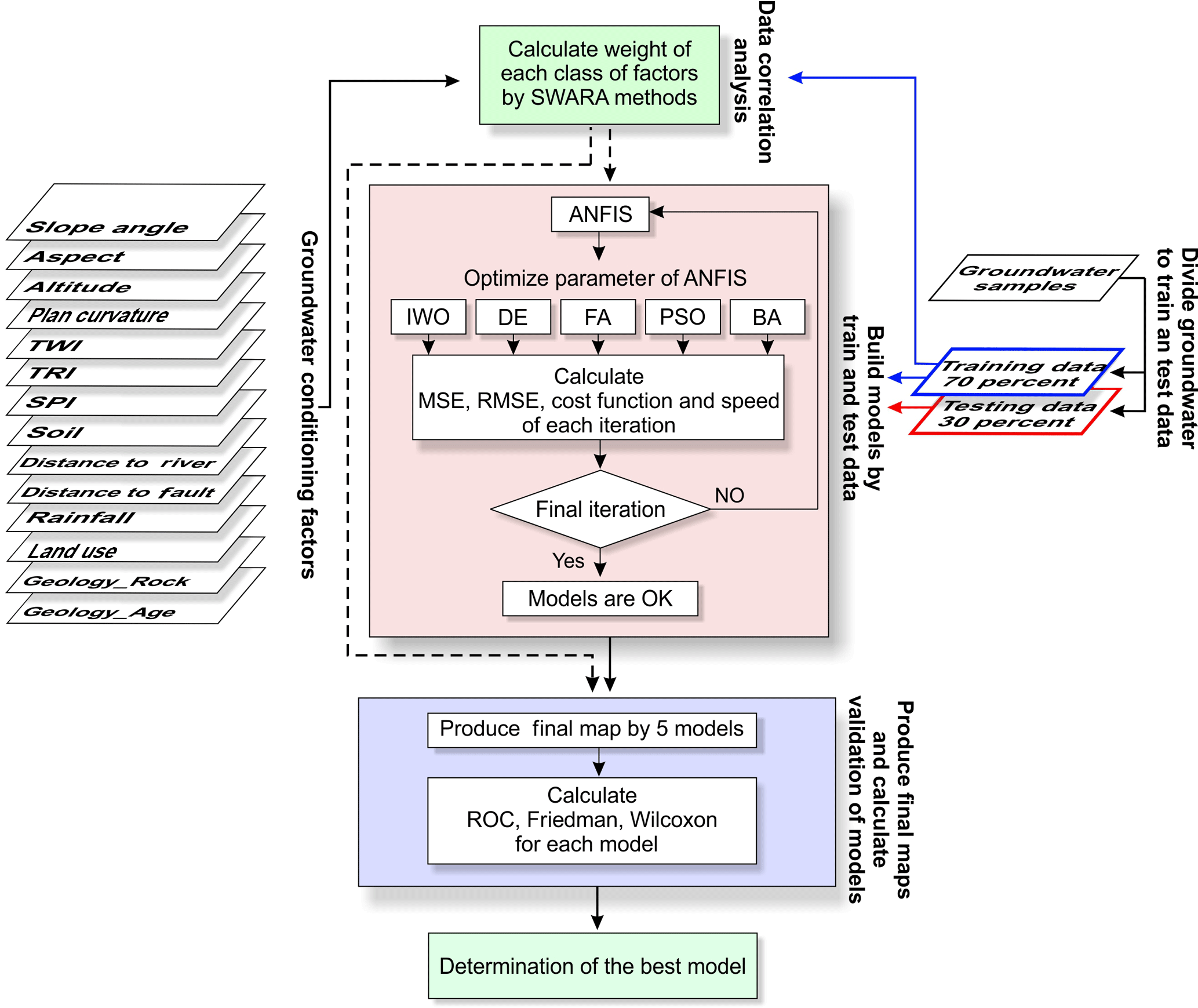
An overview of the methodological approach is shown in Fig. 2.
3.1 Data preparation
3.1.1 Groundwater spring inventory map
In groundwater modeling, spatial relationships between groundwater springs and conditioning factors should be analyzed and assessed to determine the best subset of these factors. In the Koohdasht–Nourabad plain, a total of 2463 spring locations were provided by the Iranian Water Resources Management Company. Most of these spring locations were checked during extensive field surveys using a handheld GPS unit.
3.1.2 Construction of the training and testing datasets
Spatial prediction of groundwater potential mapping using a machine learning model is considered a binary classification with two classes, spring and non-spring. Therefore, a total of 2463 non-spring locations were randomly generated using the random point tool in ArcGIS10.2. According to Chung and Fabbri (2003), it is possible to validate the model performance using a cross-validation method that splits the dataset into the two parts of spring and non-spring locations. The first part is used for model building, which is called a training dataset, and the other part is utilized for validation of the model performance, called a testing dataset (Pham et al., 2017a). In this study, a ratio of 70 ∕ 30 was selected randomly for generating the training and testing datasets (Pourghasemi et al., 2012, 2013a, b; Xu et al., 2012). Accordingly, both spring locations and non-spring locations have been randomly divided into two groups for training (1725 locations) and validating (738 locations) purposes (Fig. 1).
Both the training and the testing datasets were converted to a raster format, whereby spring pixels were assigned “1” and non-spring pixels were assigned “0” (Bui et al., 2015), and then, these pixels were overlaid with 13 groundwater conditioning factors to extract their attribute values.
3.1.3 Groundwater conditioning factor analysis
Selection of the groundwater conditioning factors
After the initial selection of the conditioning factors, these factors should be assessed for multicollinearity problems. Multicollinearity takes place when two or more independent conditioning factors are highly correlated, or, in other words, interdependent (Li et al., 2010). Several methods have been proposed to diagnose multicollinearity, and among them, the variance inflation factor (VIF) and tolerance (TOL) are widely used in environmental modeling (O'brien, 2007; Bui et al., 2016); therefore, they were selected for this research. Factors with VIFs greater than 5 and TOL less than 0.1 indicate that multicollinearity problems existed (O'brien, 2007; Bui et al., 2011). Another method, namely the information gain ratio (IGR) technique, was applied to identify the relative importance of the conditioning factor and also to obtain factors with null effect. These factors must be removed to increase the accuracy of the model (Khosravi et al., 2018).
In the current study, 13 conditioning factors have been selected, namely the slope degree, slope aspect, altitude, plan curvature, stream power index (SPI), topographic wetness index (TWI), terrain roughness index (TRI), distance from fault, distance from river, land use/land cover, rainfall, soil order, and lithology units. These factors have been determined based on a literature review, characteristics of the study area, and data availability (Nampak et al., 2014; Mukherjee, 1996; Oh et al., 2011; Ozdemir, 2011b). The process of converting continuous variables into categorical classes was carried out based on our frequency analysis of spring location (Khosravi et al., 2018) in order to define the class intervals.
A digital elevation model (DEM) of the study area was downloaded from ASTER Global DEM (https://asterweb.jpl.nasa.gov/gdem.asp, last access: 20 April 2017) with a grid size of 30×30 m. Based on the DEM, slope degree, slope aspect, altitude, plan curvature, SPI, TWI, and TRI were derived. Slope degree has been divided in five categories using the quantile classification scheme (Tehrany et al., 2013, 2014), namely 0–5.5, 5.5–12.11, 12.11–19.4, 19.4–28.7, and 28.7–64.3∘ (Fig. 3a). Slope aspect is selected because it controls solar radiation budgets that influence the groundwater potential. Slope aspect has been provided in five different classes, flat, north, west, south, and east (Fig. 3b). Altitude was divided into five classes using the quantile classification scheme, namely 531–1070, 1070–1385, 1385–1703, 1703–2068, and 2068–3175 m (Fig. 3c). Plan curvature was divided into three classes, namely concave (), flat (−0.05 to 0.05), and convex (>0.05) (Fig. 3d) (Pham et al., 2017a).
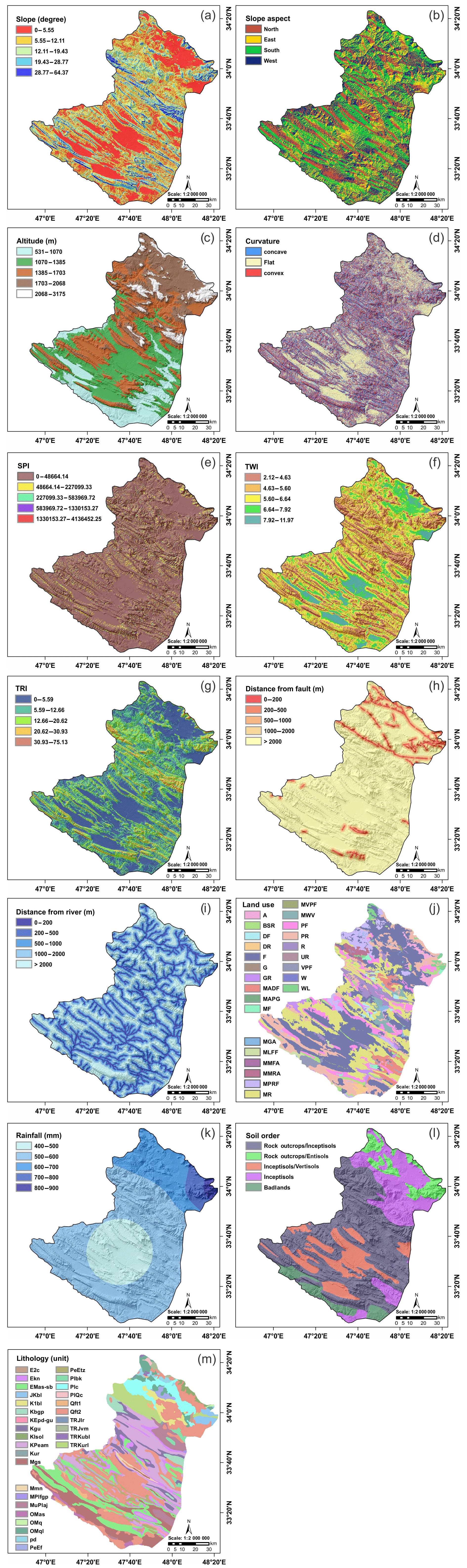
Figure 3Groundwater conditioning factors for the study area used in this research: (a) slope degree, (b) slope aspect, (c) altitude, (d) plan curvature, (e) SPI, (f) TWI, (g) TRI, (h) distance from fault, (i) distance from river, (j) land use/land cover, (k) rainfall, (l) soil order, and (m) lithology units.
SPI is related to the erosive power of surface runoff, whereas TWI relates to the amount of the flow that accumulates at any point in the catchment. In this research, SPI, TWI, and TRI were constructed using the System for Automated Geoscientific Analyses (SAGA) GIS 2.2 software, and finally, were divided into five classes. These classes are 0–48 664, 48 664–227 099, 227 099–583 969, 583 969–1 330 153, and 1 330 153–4 136 452 for SPI (Fig. 3e). For TWI, these classes are 2.1–4.6, 4.6–5.6, 5.6–6.6, 6.6–7.9, and 7.9–11.9 (Fig. 3f), and for TRI, these classes are 0–8.7, 8.7–18.2, 18.2–29.9, 29.9–46.6, and 46.6–185 (Fig. 3g).
Distances from the fault and river for the study area were generated with five classes using the Multiple Ring Buffer tool in ArcGIS 10.2, 0–200, 200–500, 500–1000, 1000–2000, and >2000 m (Fig. 3h and i). Lithology plays a key role in determining the groundwater potential due to different infiltration rates of formation (Adiat et al., 2012; Nampak et al., 2014). Land use/land cover of the study area was obtained using Landsat 7 Enhanced Thematic Mapper plus (ETM+) images that were downloaded from the US Geological Survey (available at https://earthexplorer.usgs.gov, last access: 1 May 2018). Accordingly, 25 land use/land cover types were recognized: agriculture (A), garden (G), dense forest (DF), good rangeland (GR), poor forest (PF), waterway (W), mixture of garden and agriculture (MGA), mixture of agriculture with dry farming (MADF), mixture of agriculture with poor garden (MAPG), dry farming (DF), fallow (F), dense rangeland (DR), very poor forest (VPF), mixture of waterway and vegetation (MWV), mixture of moderate forest and agriculture (MMFA), mixture of moderate rangeland and agriculture (MMRA), mixture of poor rangeland and fallow (MPRF), mixture of low forest and fallow (MLFF), woodland (WL), moderate forest (MF), moderate rangeland (MR), poor rangeland (PR), bare soil and rock (BSR), urban and residential (UR), mixture of very poor forest (MVPF), and rangeland (R) (Fig. 3j).
Rainfall is a major source of recharge for the groundwater. In this research, 15 years (2000–2015) of mean annual rainfall data from four rain-gauge stations of the study area were used. The rainfall map (Fig. 3k) with five categories (300–400, 400–500, 500–600, 600–700, and 700–800 mm) was generated using an inverse distance weighting method due to a lower root mean square error (RMSE; Khosravi et al., 2016a, b). A soil map at a scale of 1 : 50 000 for the study area was provided by the Iranian Water Resources Department (IWRD). The soil types are soil rock outcrops/Entisols, rock outcrops/Inceptisols, Inceptisols, Inceptisols/Vertisols, and badlands (Fig. 3l).
Lithology for the study area, at a scale of 1 : 100 000, was provided by the Iranian Department of Geology Survey (IDGS). Accordingly, 30 classes were used: OMq, PeEf, PlQc, K1bl, Plc, pd, TRKubl, TRJvm, MPlfgp, OMql, Plbk, E2c, TRKurl, Qft2, MuPlaj, KEpd-gu, Kgu, Qft1, Ekn, KPeam, PeEtz, Kbgp, EMas-sb, Mgs, TRJlr, Klsol, JKbl, Kur, OMas, and Mmn (Fig. 3m). Finally, using ArcGIS 10.2 software, all the aforementioned groundwater conditioning factors were converted to a raster format with a grid size of 30 m×30 m for modeling purposes.
3.2 Spatial relationship between spring location and conditioning factors
To assess the spatial relationship between spring location and conditioning factors, in this research, step-wise assessment ratio analysis (SWARA) (Keršuliene et al., 2010), a multi-criteria decision-making (MCDM) analysis, was used. SWARA has received great attention in various fields in the last 5 years (Alimardani et al., 2013; Hong et al., 2018). The working principles of SWARA are briefly described as follows.
Phase one. First, the experts will define the problem-solving criteria. By using the practical knowledge of the experts, the priority for the criteria is determined and these criteria are organized in descending order.
Phase two. The following trends are employed for the estimation of the weight of the criteria.
Starting from the second criterion, the respondent explains the relative importance of the criterion j in relation to the (j−1) criterion, and for each particular criterion as well. As Keršuliene mentioned, this process specifies the comparative importance of the average value, Sj, as follows (Keršuliene et al., 2010):
where n is the number of experts, Ai explicates the offered ranks for each factor by the experts, and j stands for the number of the factor.
Subsequently, the coefficient Kj is determined as follows:
Recalculation of weight Qj is done as follows:
The relative weights of the evaluation criteria are calculated by the following equation:
where Wj shows the relative weight of jth criterion, and m is the total number of criteria.
3.3 Groundwater spring prediction modeling
As mentioned earlier, in this research, five new metaheuristic optimization algorithms (IWO, DE, FA, PSO, and BA) were investigated in order to optimize the parameters of ANFIS. This section briefly presents the theoretical background of these algorithms and ANFIS.
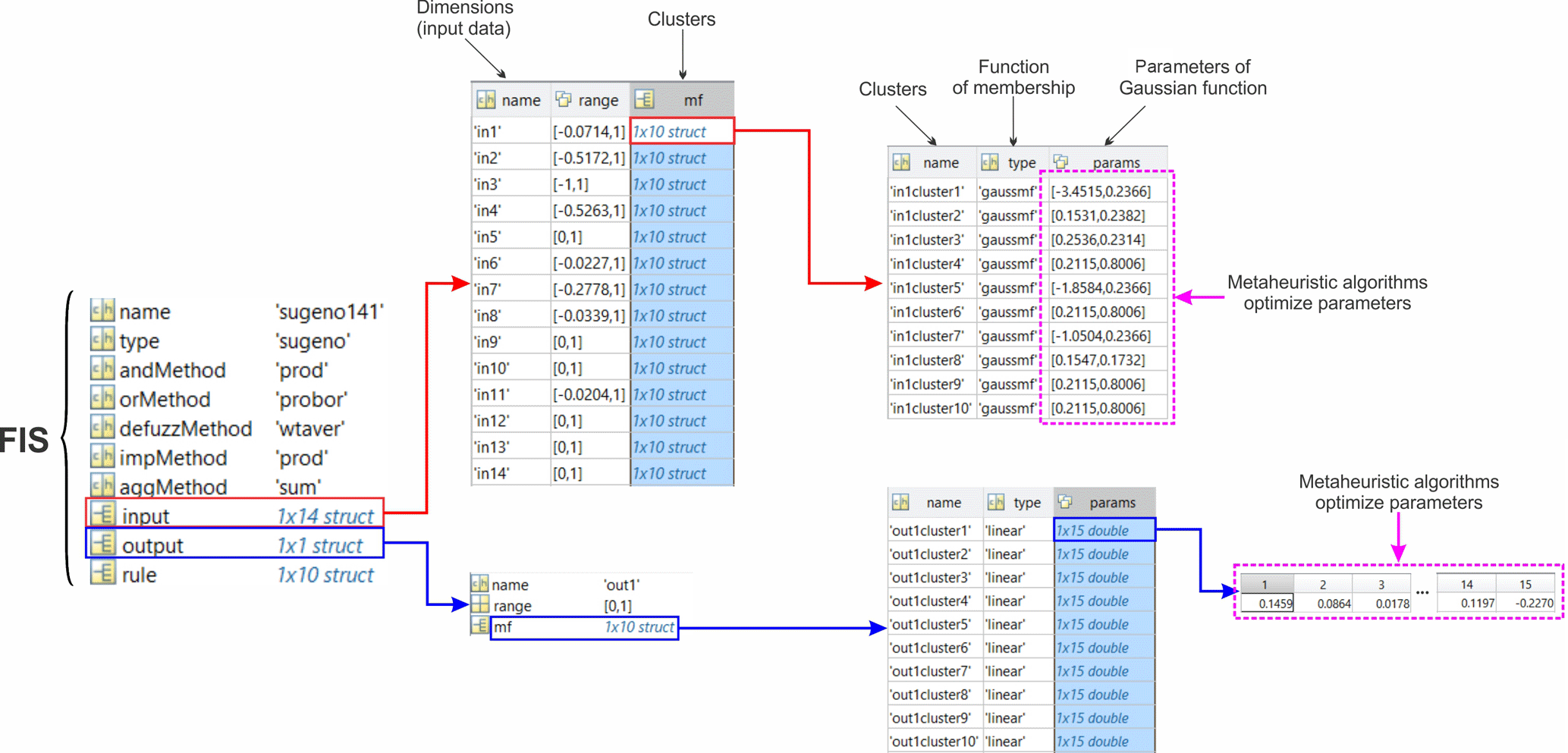
3.3.1 Adaptive neuro-fuzzy inference system
An adaptive neuro-fuzzy inference system (ANFIS) was proposed by Jang (1993) to solve nonlinear and complex problems in one framework. ANFIS converts input data to fuzzy inputs by using a membership function; there are different membership functions that describe system behavior (Jang, 1993). ANFIS is applied to the Takagi–Sugeno–Kang (TSK) fuzzy model with two “if-then” rules, both with two inputs, x1 and x2, and one output, f (Takagi and Sugeno, 1985), as follows:
Jang's ANFIS consists of a feed-forward neural network with six distinct layers. Detailed description of ANFIS can be found in Jang (1993).
3.3.2 Metaheuristic optimization algorithms
The main goal of these algorithms is to find the optimal antecedent and the consequent parameters of the ANFIS model using IWO, DE, FA, PSO, and BA algorithms. Figure 4 illustrates a general methodological data flow of the ANFIS model.
Invasive weed optimization algorithm
Invasive weed optimization (IWO) mimics the colonizing behavior of weeds. Its design, by Mehrabian and Lucas (2006), is based on the way that weeds find proper space for growth and reproduction. One characteristic of this algorithm is its simple structure; the number of input parameters is low and it has strong robustness. Furthermore, it is easy to understand and the same merit causes it to be used for solving difficult nonlinear optimization problems (Ghasemi et al., 2014; Naidu and Ojha, 2015; Zhou et al., 2015). This algorithm consists of four parts: initialization, reproduction, spatial dispersal, competitive exclusion, and termination condition.
Differential evolution algorithm
Differential evolution (DE) is an evolutionary algorithm for finding global optimal answers for problems with continuous space (Das et al., 2009). This algorithm starts by producing a random population in which each individual of the population is a solution to the problem. Vector shows each individual of the population, is a number denoting each individual, in which D stands for the search dimension, or in other words, is a component problem, and generation time, where Gmax is the total number of generations.
By assuming the maximum and minimum of every dimension of searching space, there are and , respectively; initial population is defined by the following (Storn and Price, 1997):
where rand (0, 1) is a uniformly distributed random number in [0,1]. Detailed description of DE can be found in Chen et al. (2017).
Firefly algorithm
The firefly algorithm (FA) is as a metaheuristic algorithm, proposed by Yang (2010), that is originated from the flashing and communication behavior of fireflies. Like other swarm intelligence algorithms, of which components are known as solutions to the problems, in this algorithm, each firefly is a solution and its light intensity is the objective function value. In general, the FA follows three idealized rules as given below: (1) all firefly species are unisex, with each of them attracting other fireflies without considering their gender (Amiri et al., 2013); (2) attractiveness of a firefly is related to its light intensity, and thus, from two flashing firefly species, one with lower light intensity moves toward the other one with higher light intensity; (3) light intensity of a firefly is defined as an objective function value and must be optimized.
Particle swarm optimization algorithm
The article swarm optimization (PSO) algorithm has been inspired by the way birds use their collective intelligence for finding the best way to get food (Kennedy and Eberhart, 1995). Each bird implemented in this algorithm acts as a particle that is in fact a representative of a solution to the problem. These particles find the optimum answers for the problem by searching in “n” dimensional space, and “n” is the number of the problem's parameters. For this purpose, particles were scattered randomly in space at the beginning of algorithm execution. Detailed description of PSO can be found in Kennedy (2011).
Bees algorithm
The bees algorithm (BA), which was introduced by Pham et al. (2005), is inspired by the foraging behavior of bees' colonies in search of food sources located near the hive. In the initial setup, evenly distributed scout bees are scattered randomly in different directions to identify flower patches. After that, scout bees come back to the hive and start a specific dance called the waggle dance. This dance is for communicating with others in order to share the information of discovered flower patches. The information indicates direction, distance, and nectar quality of the flower patches, and helps the colony to have proper evaluation of all flower patches. After evaluation, scout bees come back to the location of discovered flower patches with other bees, named recruit bees. Dependent on the distance and the amount of nectar, a different number of recruit bees is assigned to each flower patch. In other words, those flower patches with better nectar quality are designated more recruit bees. Recruit bees then evaluate the quality of flower patches when performing the harvest process, and leave the flower patches with a low quality. Conversely, if the flower patch quality is good, it will be announced during the next waggle dance.
3.4 Performance assessment of models
According to Chung and Fabbari (2003), without validation, the results (achieved maps) of the models do not have any scientific significance. Prediction capability of these five spatial groundwater models must be evaluated using both success-rate curves and prediction-rate curves (Hong et al., 2015). Success-rate curves show how suitable the built model is for groundwater potential assessment (Gaprindashvili et al., 2014). Success-rate curves have been constructed using groundwater potential maps and the number of spring locations used in the training dataset (Tien Bui et al., 2012). Prediction-rate curves constructed using the testing dataset demonstrate how good the model is and evaluate the prediction power of the models. Therefore, it can be used for model prediction capabilities (Brenning, 2005). The area under the curve (AUC) of success and prediction rate is the basis for assessing the accuracy of the groundwater potential models quantitatively (Khosravi et al., 2016a, b; Pham et al., 2017b). The AUC value varies from 0.5 to 1; the higher the AUC, the better the prediction capability of models (Tien Bui and Hoang, 2018; Ngoc-Thach et al., 2018).
In addition, the mean squared error (MSE) was further used (Bui et al., 2016) as follows:
where Oi and Ei are observation (target) and prediction (output) values in both training and testing datasets, and N is the total samples in the training or the testing dataset.
3.5 Inferential statistics
3.5.1 Friedman test
Nonparametric statistical procedures such as the Friedman test (Friedman, 1937) can be used regardless of statistical assumptions (Derrac et al., 2011) and do not presuppose the data to be normally distributed. The main aim of this test is to find whether there is a significant difference between the models' performance or not. In other words, multiple comparisons are performed to detect significant differences between the behaviors of two or more models (Beasley and Zumbo, 2003). The null hypothesis (H0) is that there are no differences among the performances of the groundwater potential models. The higher the p value, the higher the probability that the null hypothesis is not true, since if the p value is less than the significance level (α=0.05), the null hypothesis will be rejected.
3.5.2 Wilcoxon signed-rank test
Because the Friedman test only illustrates whether there is any difference between the models or not, this test does not provide pairwise comparisons among compared models. Therefore, another nonparametric statistical test named the Wilcoxon signed-rank test has been applied. To evaluate the significance of differences between the performances of groundwater potential models, the p value and z value have been used.
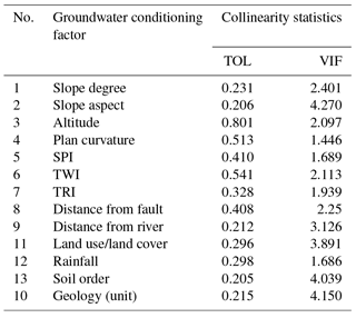
4.1 Multicollinearity diagnosis
Results of the multicollinearity analysis in this study are shown in Table 1. The analysis revealed that as the VIF is less than 5 and TOL is greater than 0.1, no multicollinearity problems exist among conditioning factors.
4.2 Determination of the most important parameters
The most common method, the information gain ratio (IGR), was applied to identify the most important conditioning factors. Result shows that all 13 conditioning factors affect groundwater occurrence. The land use/land cover factor has the most important impact on groundwater (IGR = 0.502), followed by lithology (IGR = 0.465), rainfall (IGR = 0.421), TWI (IGR = 0.400), soil (IGR = 0.370), TRI (IGR = 0.337), slope degree (IGR = 0.317), altitude (IGR = 0.287), distance to river (IGR = 0.139), aspect (IGR = 0.066), plan curvature (IGR = 0.0548), distance to fault (IGR = 0.0482), and SPI (IGR = 0.0323).
4.3 Spatial relationship between springs and conditioning factors using the SWARA method
The spatial correlation between groundwater springs and the conditioning factors is shown in Table 2. Regarding the slope, the class of 0–5.5∘ shows the highest probability (0.45) of groundwater spring occurrence. As the slope degree increases, the probability of spring occurrence is reduced. In the case of slope aspect, the east aspect (0.44) has the most impact on spring occurrence. According to calculated results, in terms of altitude, springs are the most abundant in altitudes of 1703–2068 m (0.6). The SWARA model is high in flat areas (0.4), followed by areas with concave (0.38) and convex (0.2) curvature. For SPI, the highest SWARA value is found for the classes of 583 969–1 330 153 (0.46). In the case of the TWI, the SWARA values decrease when the TWI reduces. There is an inverse relationship between TRI and SWARA values, and as the TRI increases, the SWARA value reduces.
Table 2Spatial correlation between the conditioning factors and spring locations using the SWARA method.
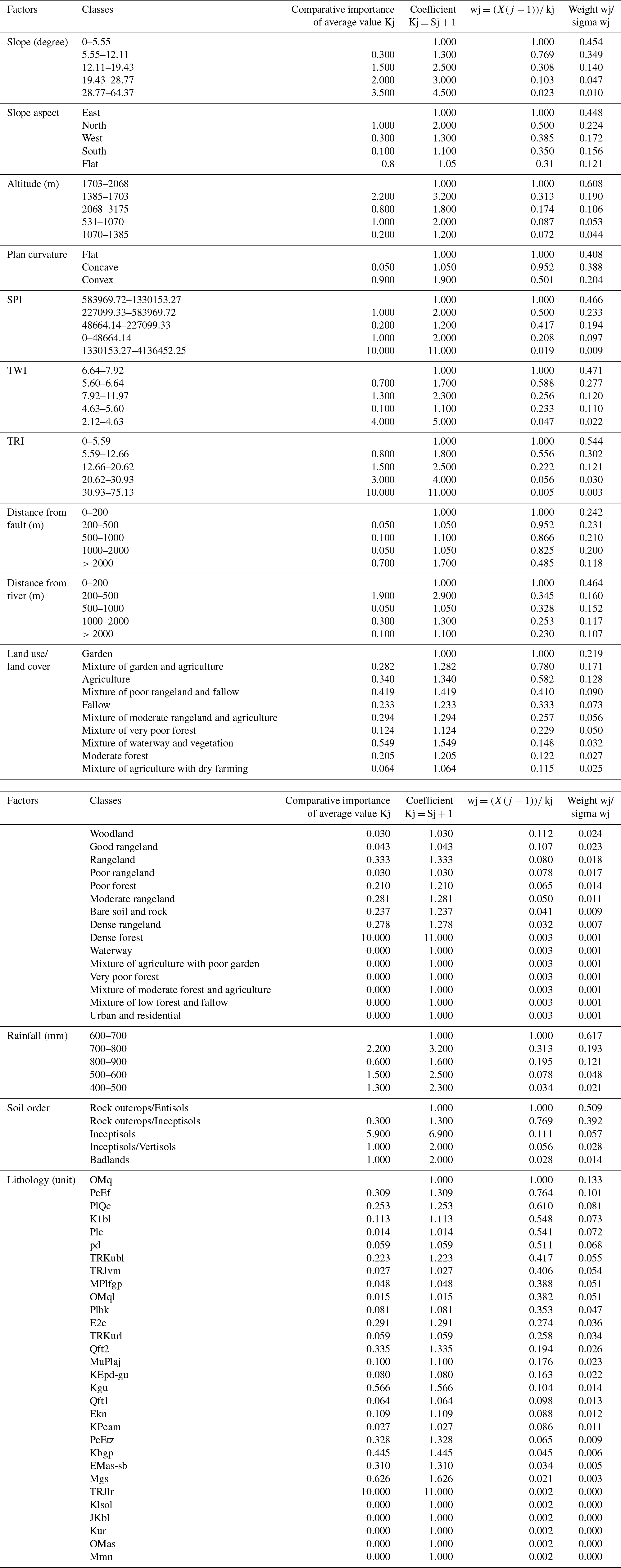
Regarding distance from the fault, a distance less than 2000 m has the highest impact on spring occurrence, and with an increase in distance (greater than 2000 m), the probability of spring occurrence is reduced. Regarding distance to river, it can be seen that the class of 0–200 m has the highest correlation with spring occurrence (0.46) and there is an inverse relationship between spring occurrence and SWARA values. In the case of land use, the highest SWARA values are shown for garden areas (0.219), followed by a mixture of garden and agriculture (0.17) and agricultural areas (0.12), whereas the lowest SWARA is for bare soil and rock (0.00063). Rainfall between 500 and 600 mm has the highest SWARA value (0.61). The Inceptisols class has the highest SWARA values (0.5), followed by rock outcrops/Entisols (0.39), rock outcrops/Inceptisols (0.056), Inceptisols/Vertisols (0.028), and badlands (0.014). The highest probability is shown for the highly porous and very good water reservoir karstic Oligo-Miocene and Cretaceous pure carbonate formation (OMq and K1bl), the young and poorly consolidated highly porous detrital rock units (PeEf and Plq), and the unconsolidated Quaternary alluvium (PlQc).
4.4 Application of ANFIS ensemble models and their assessment
In the current study, hybrids of the ANFIS model and five metaheuristic algorithms were designed, constructed, and implemented in MATLAB 8.0 software. These models were built using the training dataset. Weights gained by the SWARA method for each conditioning factor were fed as input into the training dataset. The results are shown in Figs. 5 and 6.
As can be seen in Fig. 5, the MSEs of the ANFIS–IWO model, the ANFIS–DE model, the ANFIS–FA model, the ANFIS–PSO model, and the ANFIS–BA model using the training dataset are 0.066, 0.066, 0.066, 0.049, and 0.09, respectively. This indicates that the ANFIS–PSO model has the highest performance, whereas the ANFIS–BA model presents the lowest one. The prediction performance of the five models using the validation dataset is shown in Fig. 6. MSEs of the ANFIS–IWO model, the ANFIS–DE model, the ANFIS–FA model, the ANFIS–PSO model, and the ANFIS–BA model are 0.060, 0.060, 0.060, 0.045, and 0.09, respectively. Therefore, it could be concluded that the ANFIS–PSO model and ANFIS–BA model have the highest and lowest prediction performances, respectively.
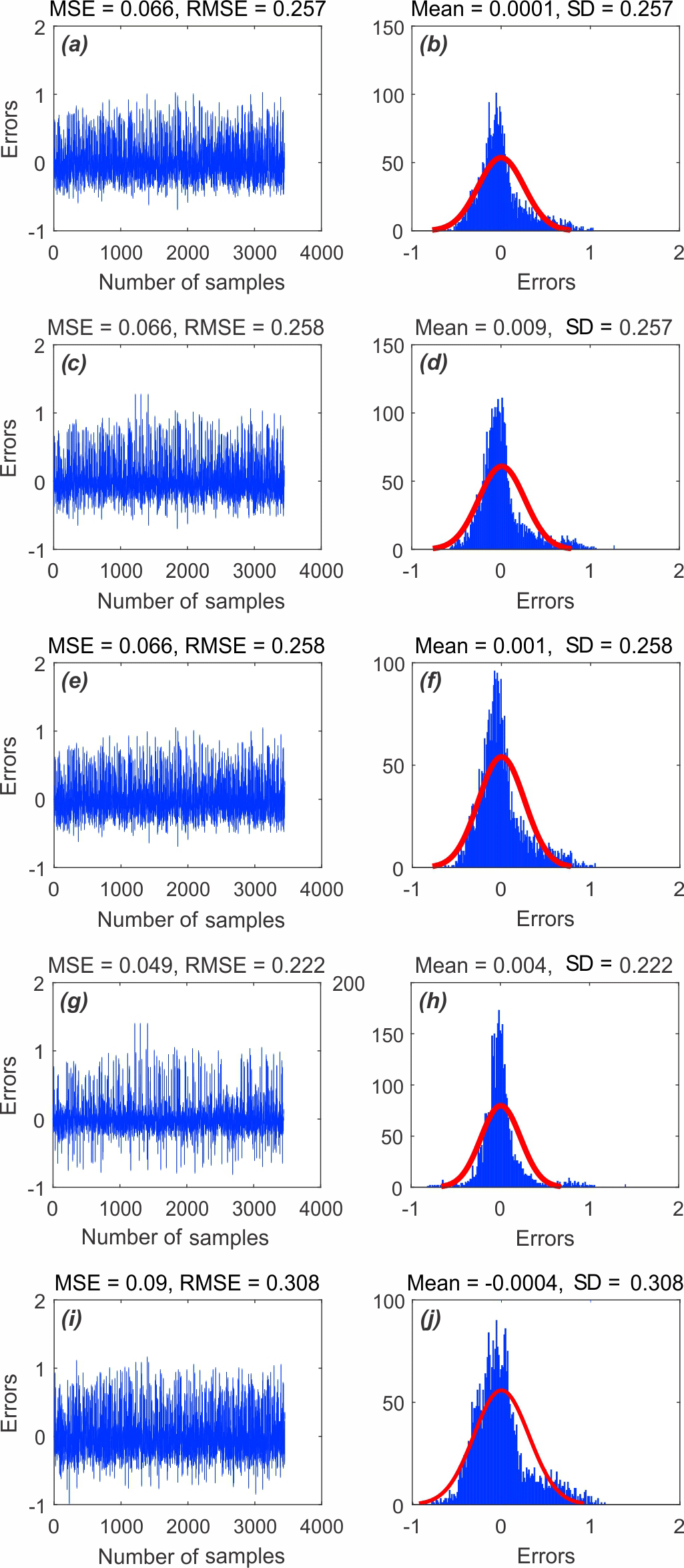
Figure 5MSE and RMSE values of the five models using the training dataset of (a) ANFIS–IWO, (c) ANFIS–DE, (e) ANFIS–FA, (g) ANFIS–PSO, and (i) ANFIS–BA. Frequency errors of the five models using the train dataset of (b) ANFIS–IWO, (d) ANFIS–DE, (f) ANFIS–FA, (h) ANFIS–PSO, and (j) ANFIS–BA.
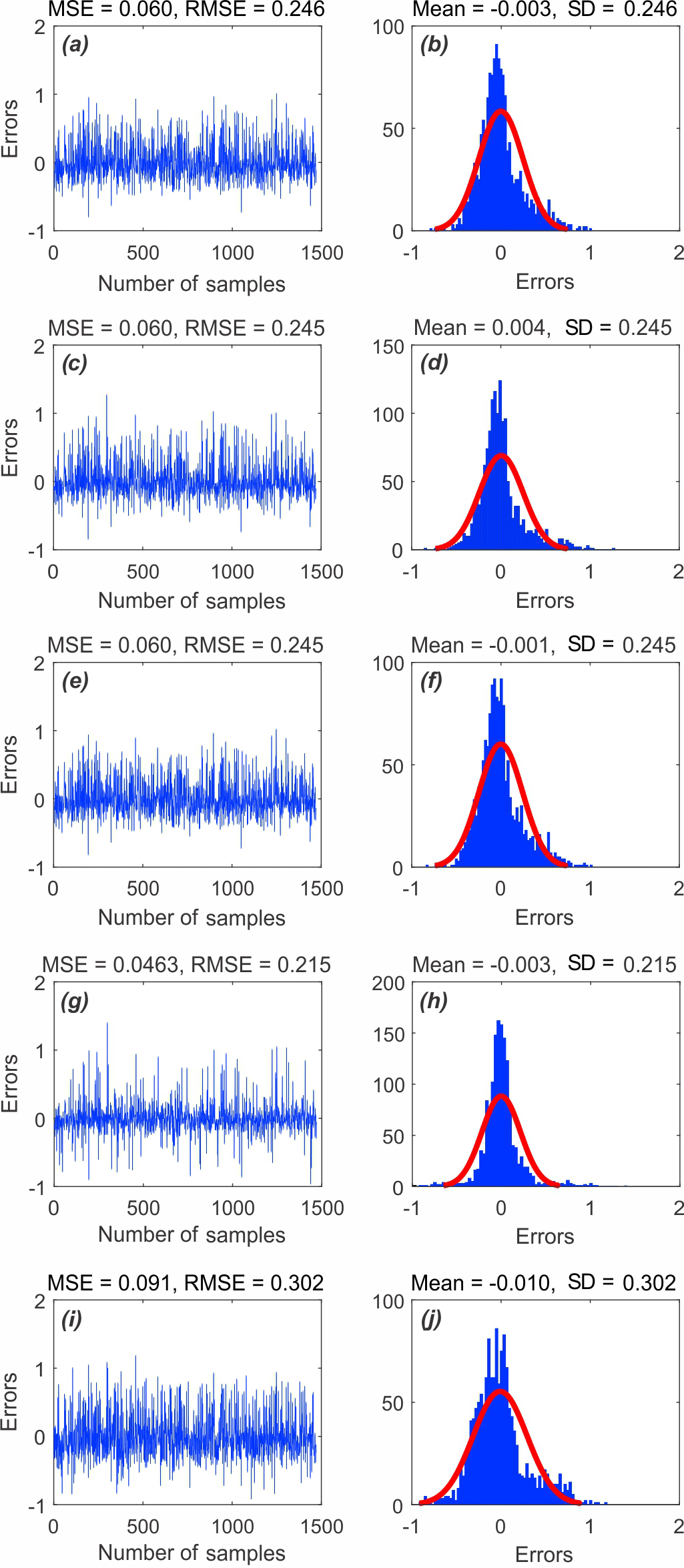
Figure 6MSE and RMSE values of the five models using the validation dataset of (a) ANFIS–IWO, (c) ANFIS–DE, (e) ANFIS–FA, (g) ANFIS–PSO, and (i) ANFIS–BA. Frequency errors of the five models using the validation dataset of (b) ANFIS–IWO, (d) ANFIS–DE, (f) ANFIS–FA, (h) ANFIS–PSO, and (j) ANFIS–BA.
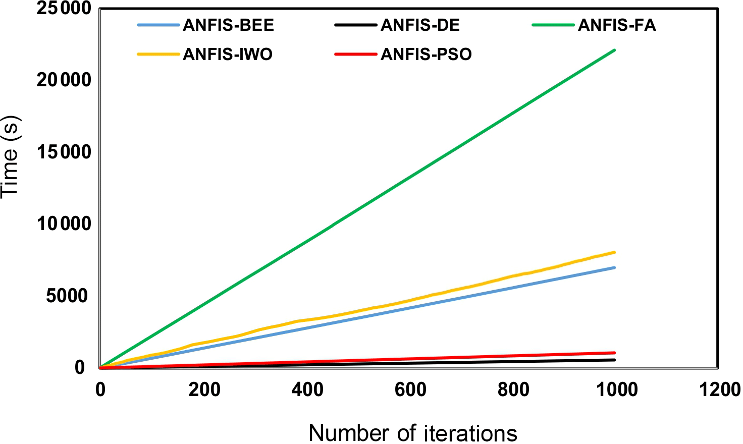
However, it should be noticed that, in addition to accuracy, the execution speed of the five models was found to be of significance. To measure this, the running time for 1000 iterations was estimated. The result is shown in Fig. 7. It could be seen that the running time of the ANFIS–IWO model, the ANFIS–DE model, the ANFIS–FA model, the ANFIS–PSO model, and the ANFIS–BA model was 8036, 547, 22 111, 1050, and 6993 s, respectively. It can be concluded that the ANFIS–DE model had the lowest running time and the ANFIS–FA model had the maximum time.
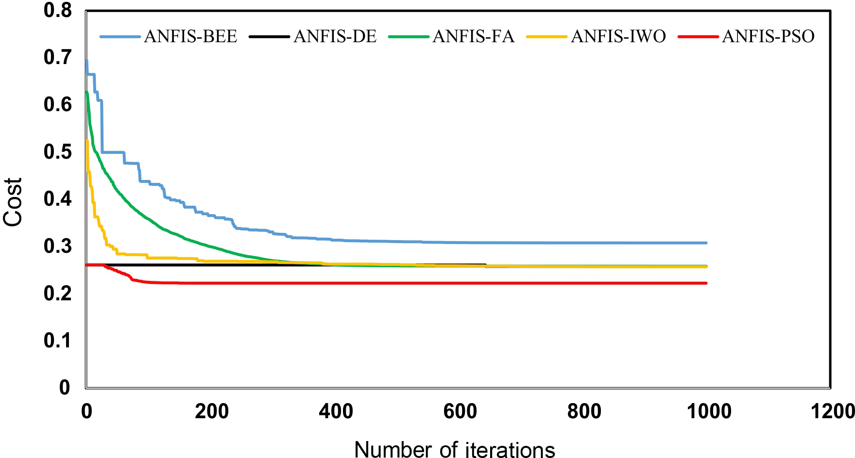
On the other hand, it is possible to test how each model achieves convergence in learning. Using the cost function values, a convergence graph for all five models was constructed and shown in Fig. 8. The results show that cost function values of the ANFIS–DE model and the ANFIS–BA model were stable from 30 and 95 iterations, indicating a rapid convergence of the models, while the ANFIS–PSO model, the ANFIS–IWO model, and the ANFIS–FA model showed a convergence after 650, 650, and 360 iterations, respectively. This indicates a slow convergence.
4.5 Generation of groundwater spring potential maps using ANFIS hybrid models
Once the five models were successfully trained and validated, these models were used to compute groundwater spring indices for all the pixels of the study areas. Then, these indices were exported from MATLAB into ArcGIS10.2 software for generating groundwater spring potential maps. Ultimately, the achieved maps could be sorted into five classes: very low, low, moderate, high, and very high (Fig. 9a–e).
Many methods can be used for determining thresholds for the five classes: manual, equal interval, geometric interval, quantile, natural break, and standard deviation. Selection of a method depends on the characteristics of the data and the distribution of the groundwater spring indexes in a histogram (Ayalew and Yamagishi, 2005). If the indexes have a positive or negative skewness, the quantile or natural break classification is suitable for index classification (Akgun, 2012). In this research, the histogram was checked and the results revealed that the quantile method was better than other methods for index classification.
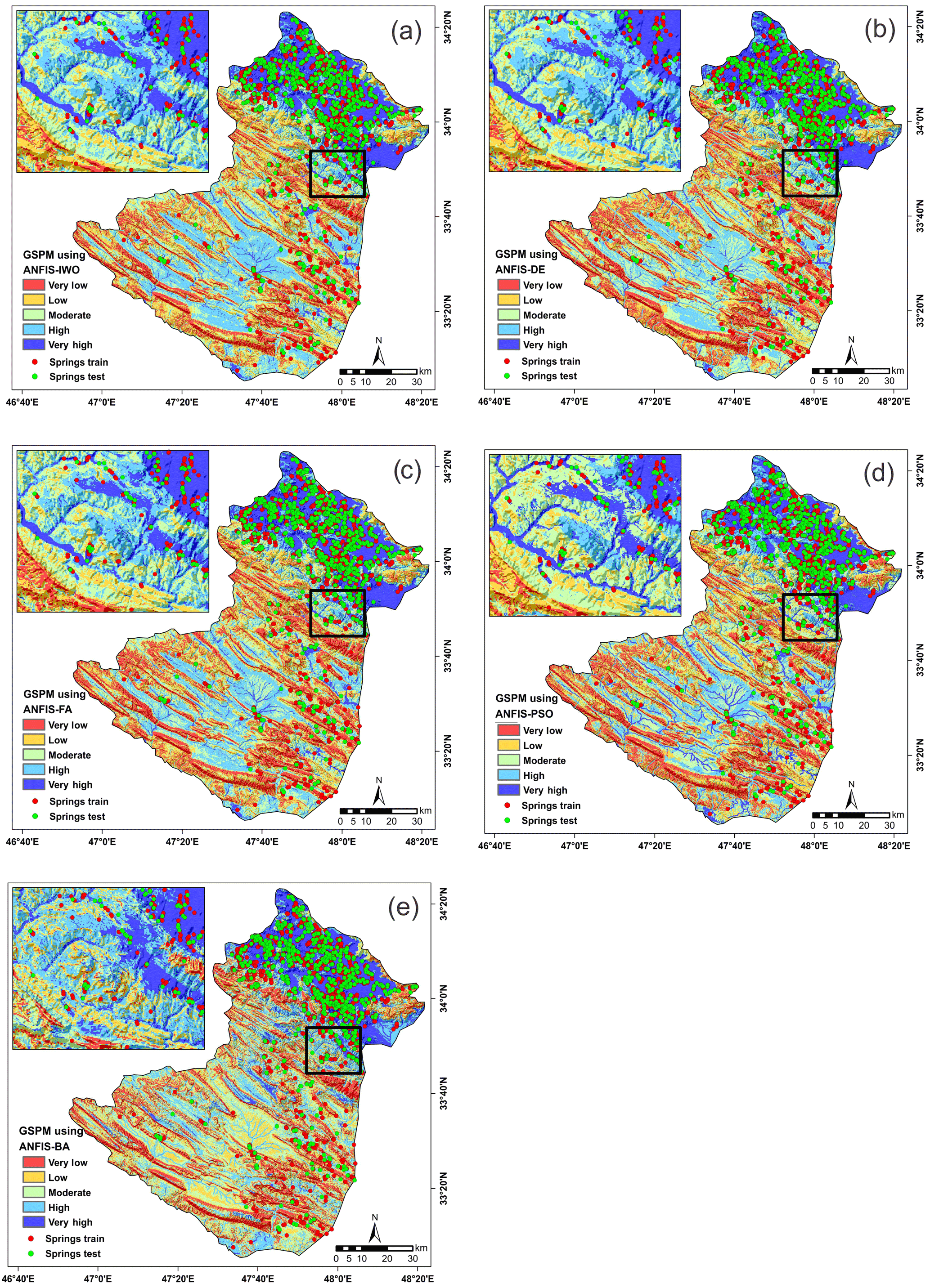
Figure 9Groundwater spring potential map using (a) the ANFIS–IWO model, (b) the ANFIS–DE model, (c) the ANFIS–FA model, (d) the ANFIS–PSO model, and (e) the ANFIS–BA model.
4.6 Validation and comparisons of the groundwater spring potential map
The prediction ability and reliability of the five achieved maps have been evaluated using both the training and the validation datasets. The results of the success rate revealed that the ANFIS–DE model had the highest AUC value (0.883), followed by the ANFIS–IWO model (0.882), the ANFIS–FA model (0.882), the ANFIS–PSO model (0.871), and the ANFIS–BA model (0.852) (Fig. 10a). Regarding the prediction rate, all five models had a good prediction capability but the ANFIS–DE model has the highest prediction rate (0.873), followed by the ANFIS-IWO model (0.873) and the ANFIS–FA model (0.873), the ANFIS–PSO model (0.865), and the ANFIS–BA model (0.839)(Fig. 10b).

4.7 Statistical tests
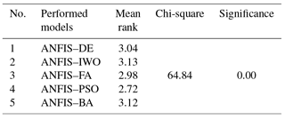
The result of the Friedman test (Table 3) revealed that as significance and chi-square values were less than 0.05 and greater than 3.84, respectively, the null hypothesis was rejected. The result also indicated that there was a statistically significant difference between prediction capabilities of the five models.
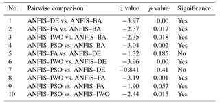
The results of the Wilcoxon signed-rank test showed that both p values and z values were far from the standard values of 0.05 and from −1.96 to +1.96, respectively, except for the ANFIS–FA model vs. the ANFIS–DE model and the ANFIS–PSO model vs. the ANFIS–DE model (Table 4). This indicates that there are statistically significant differences between models' performance, except for ANFIS–FA vs. ANFIS–DE and ANFIS–PSO vs. ANFIS–DE.
4.8 Percentage area
The percentage area of each class of final map resulting from the five hybrid models is shown in Fig. 11. According to the results of the ANFIS–DE, the most accurate model in groundwater spring potential mapping, the percentage areas of very low, low, moderate, high, and very high groundwater spring potential are about 19.06, 19.88, 21.72, 20.55, and 18.78 % of the study area, respectively.
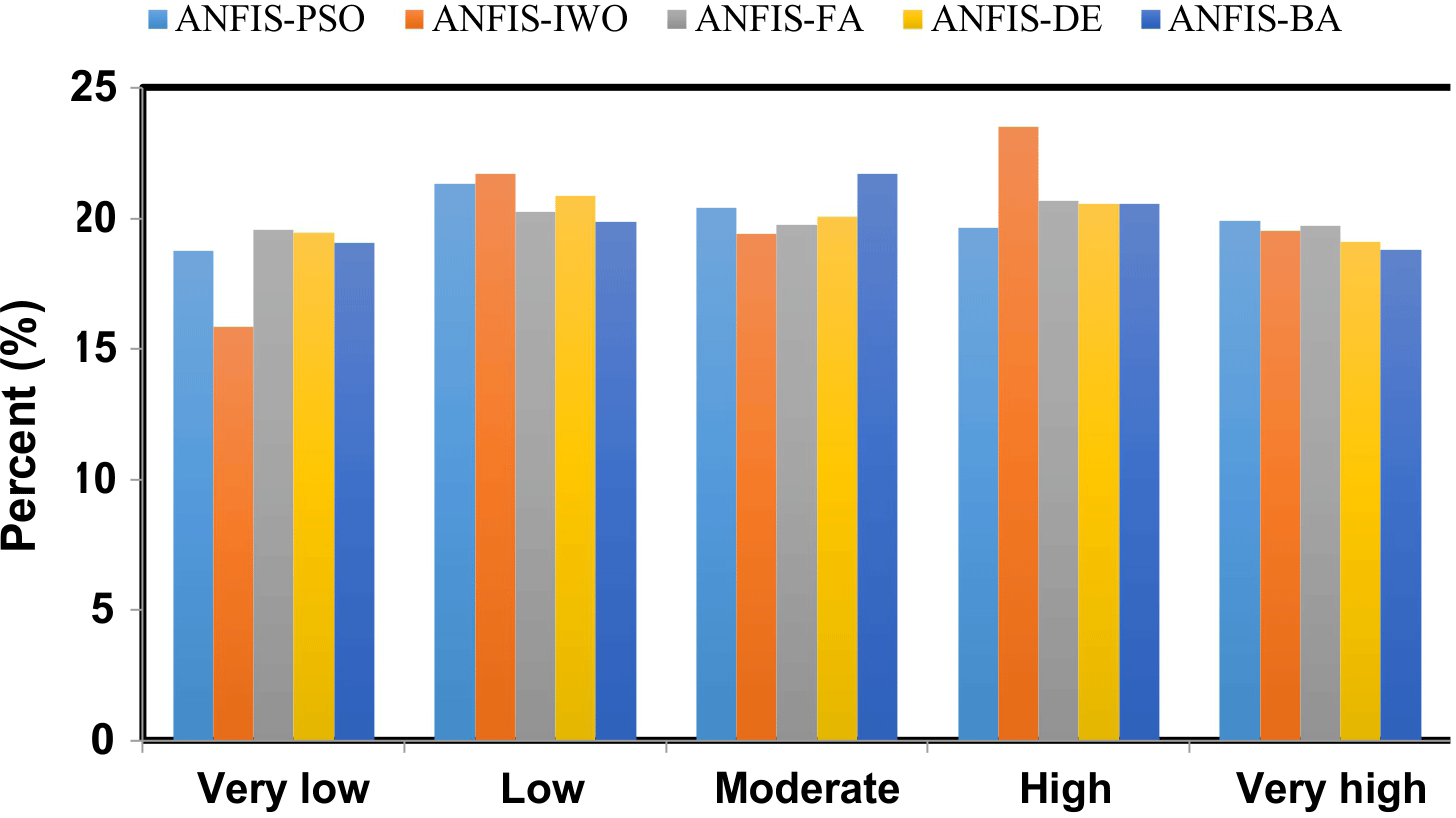
Figure 11Percentage areas of different groundwater spring potential classes for five models.
5.1 The impact of conditioning factor classes on GSPM
Assessment of conditioning factor is a necessary step in finding the correlation analysis between the groundwater spring and the conditioning factors. It should be noted that no universal guideline is available regarding the number and size of the classes as well as the selection of the conditioning factors. They were selected mostly based on characteristics of the study area and previous similar studies (Xu et al., 2013). As the slope increases, the probability of water infiltration reduces and runoff generation will increase. Thus, the steeper the slope, the lower the spring occurrence probability. According to the results of the SWARA method, the springs tend to occur at middle altitudes or on mountain slopes. Land in the flat curvature class retains rainfall which then infiltrates. Therefore, the amount of groundwater in these areas is higher than for concave or convex curvature. The east aspect has more springs than other aspects. These results are in accordance with Pourtaghi and Pourghasemi (2014), who reported that most springs occurred at elevations of 1600–1900 m with an east slope aspect (using the FR method).
TWI shows the amount of wetness, and it is obvious that the more the TWI, the higher the groundwater springs probability occurrence is. The terrain roughness index (TRI), or topographic roughness or terrain ruggedness, calculates the sum of change in elevation between a grid cell and its neighborhood, and the lesser the roughness, the higher the spring potential mapping. The SPI shows that the erosive power of the water and the mountainous area is higher than the plain area. So, as the SPI increases, the spring potential occurrence increases. Rivers are one of the most important sources of groundwater recharge, and the nearer to river, the higher the probability of spring occurrence. Also, as the rainfall increases, the groundwater spring incidence increases, but in the current study, some other conditioning factors affected the spring occurrence.
Most of the springs were located in the garden land use/land cover category. Therefore, it can be stated that the gardens have been established near the springs. Pliocene–Quaternary formation is newer on a geologic timescale, and Quaternary formation has a higher potential for groundwater spring incidence due to high permeability. A fault causes discontinuity in a volume of rock. Thus, the nearer to the fault, the higher the spring occurrence probability will be. Inceptisols soils are relatively new and are characterized as only having a weak appearance of horizons. They are the most abundant on the Earth (https://www.britannica.com/science/Inceptisol, last access: 1 May 2018) and are mostly formed from colluvial and alluvial materials. So, due to high permeability and high rainfall infiltration, they have a high potential for spring occurrence. In the case of lithological units, there are four suitable rock types in a water reservoir based on physical phenomena such as porosity and permeability that consist of (1) unconsolidated sands and gravels, (2) sandstones, (3) limestones, and (4) basaltic lava flows. In this study area lithological units include sedimentary rocks, mostly carbonate and detrital rocks, with cover of alluvium and minor soil.
5.2 Advantages/disadvantages of the models and performance analysis
The highest accuracy based on the MSE in both the training and validation datasets is found for the ANFIS–PSO model. However, based on the AUC of the success rate and the prediction rate, the ANFIS–DE model has the highest performance. The problem with the MSE comes from the fact that it is based on the error assessment. But the models should be acted upon holistically based on abilities. The AUC is based on the true positive (TP), true negative (TN), false positive (FP), and false negative (FN) (Pham et al., 2018b), and therefore is more accurate than the RMSE for comparison (Termeh et al., 2018).
ANFIS has the potential to capture the benefits of both a neural network and fuzzy logic in a single framework and can be considered to be a robust model. ANFIS had some advantages including the following: (1) a much better learning ability, (2) a need for fewer adjustable parameters than those required in other neural network structure, (3) the allowance of a better integration with other control design methods through its networks, and (4) more flexibility (Vahidnia et al., 2010).
Despite several advantages of ANFIS, determination of the membership function is the biggest disadvantage of this model. Finding the optimal parameter for a neural fuzzy model in a membership function is difficult; therefore, the best parameter should make use of other optimization models. This problem was addressed in this paper by being solved using five metaheuristic algorithms, namely IWO, DE, FA, PSO, and BA.
In the current study, the results showed that DE algorithm optimized the parameter for the neural fuzzy model better than the four other algorithms. The main DE algorithm's advantage is its simplicity as it consists of only three parameters called N (size of population), F (mutation parameter), and C (crossover parameter) for controlling the search process (Tvrdýk, 2006). Advantages of the DE algorithm can be explained as follows: (1) ability to handle non-differentiable, nonlinear, and multimodal cost functions, (2) parallelizability to cope with computation-intensive cost functions, (3) good convergence properties, and (4) random sampling and combination of vectors in the present population for creating vectors for the next generation.
Finally, it should be noted that each algorithm has some advantages or disadvantages according to the optimization problems which can be summarized as follows.
Some of the advantages of IWO include the manner of reproduction, spatial dispersal, and competitive exclusion (Mehrabian and Lucas, 2006) as well as the fact that seeds and their parents are ranked together and that those with better fitness survive and become reproductive (Ahmed et al., 2014). This algorithm can benefit from combined advantages of retaining the dominant poles and the error minimization (Abu-Al-Nadi et al., 2013).
The bees algorithm does not employ any probability approach, but it utilizes fitness evaluation to drive the search (Yuce et al., 2013). This algorithm uses a set of parameters that makes it powerful, including the number of scout bees in the selected patches, the number of best patches in the selected patches, the number of elite patches in the selected best patches, the number of recruited bees in the elite patches, the number of recruited bees in the non-elite best patches, the size of neighborhood for each patch, the number of iterations and the difference between the value of first and last iterations.
The firefly algorithm's advantages are summarized as (1) the handling of highly nonlinear, multimodal optimization problems efficiently, (2) non-utilization of velocities, (3) its ability to be integrated with other optimization techniques as a flexible method, and finally (4) no need of a good initial solution to begin its iteration process.
Advantages of the particle swarm optimization (PSO) algorithm can be summarized as follows: (1) particles update themselves with the internal velocity; (2) particles have a memory, which is important for the algorithm; (3) the “best” particle gives out the information to others; (4) it often produces quality solutions more rapidly than alternative methods; and (5) it automatically searches for the optimum solution in the solution space (Wan, 2013).
As a result, there is no algorithm which works perfectly for all optimization problems, and each algorithm has a different performance accuracy based on different data. New algorithms, therefore, should be applied and tested, and finally the most powerful algorithm should be selected as the conclusion of the research demands.
5.3 Previous works and future work proposal
Some research has been carried out on groundwater well or spring potential mapping using bivariate statistical models (Nampak et al., 2014; Guru et al., 2017; Al-Manmi and Rauf, 2016), random forests (Rahmati et al., 2016), and boosted trees for regression and classification (Naghibi et al., 2016). The ANFIS–metaheuristic hybrid models have not been used in groundwater potential mapping. However, these hybrid models have proven to be efficient in flood susceptibility mapping (Bui et al., 2016; Termeh et al., 2018) and landslide susceptibility mapping (Chen et al., 2017). Bui et al. (2016) ensemble the ANFIS using two optimization models, namely a genetic algorithm (GA) and particle swarm optimization (PSO), for the identification of flood-prone areas in Vietnam. Termeh et al. (2018) used ANFIS–ant colony optimization, ANFIS–GA, and ANFIS–PSO in flood susceptibility mapping of the Jahrom basin, and stated that ANFIS–PSO had higher prediction capabilities than the other two models. Chen et al. (2017) applied three hybrid models, namely ANFIS–GA, ANFIS–differential evolution (DE), and ANFIS–PSO, for identifying the areas prone to landslides in Hanyuan County, China. The results showed that ANFIS–DE had a higher performance (AUC = 0.84), followed by ANFIS–GA (AUC = 0.82) and ANFIS–PSO (AUC = 0.78).
In general, the results of the present study, as well as previous research, find that by applying hybrid models, better results could be achieved for spatial prediction modeling including groundwater potential mapping. The ensembles of ANFIS and metaheuristic algorithms can be applied for any spatial prediction modeling such as groundwater potential mapping, flood susceptibility mapping, landslide susceptibility assessment, gully occurrence susceptibility mapping, and other endeavors at a regional scale and in other areas.
For future work, it is recommended that (1) the water quality of the Koohdasht–Nourabad plain be investigated and the water quality of areas with high potential be determined for different aspects such as drinking and agricultural and industrial activities, and (2) the groundwater vulnerability assessment be applied by some common methods including the DRASTIC model for which the zones with a high potential for groundwater occurrence should be protected against pollution.
Groundwater is the most important natural resource in the world and about 25 % of all freshwater is estimated to be groundwater. Thus, groundwater potential mapping has been considered to be one of the most effective methods for the management of groundwater resources for better exploitation. The main results of the present study can be summarized by the following points.
- 1.
The results showed that although all models had good results, the ANFIS–DE had the highest prediction power (0.875), followed by ANFIS–IWO and ANFIS–FA (0.873), ANFIS–PSO (0.865), and ANFIS–BA (0.839).
- 2.
According to the results of the SWARA method, most springs existed in altitudes of 1703–2068 m, with a flat curvature, east aspect, TWI of 6.6–7.9, TRI of 0–8.7, SPI of 583 969–1 330 153, Inceptisols soil type, a slope of 0–5.5∘, 0–200 m distance from river, 500–1000 m distance from fault, rainfall between 500 and 600 mm, and a garden land cover category, and in a Pliocene–Quaternary lithological age with an OMq lithology unit.
- 3.
Based on the information gain ratio, the most important factors affecting groundwater occurrence are land use/land cover, lithology, rainfall, and TWI. The least important factors are plan curvature, distance to fault, and SPI.
- 4.
Based on the ANFIS–DE model, a total of 39.33 % of the study area has a high and very high groundwater potential, situated in the north.
The results of the current study are helpful for the Iran Water Resources Management Company (IWRMC) for sustainable management of groundwater resources. Overall, the maps resulting from these hybrid artificial intelligence algorithms can be applied for the better management of groundwater resources in the study area.
Data are available for download at https://github.com/mahdipan/groundwater (last access: 12 September 2018).
KK collected and processed the data, and wrote the manuscript. MP designed the experiment, performed the analysis, and wrote the manuscript. DTB checked the analysis and results, and reviewed, edited, and wrote the manuscript.
The authors declare that they have no conflict of interest.
We would like to thank Bjørn Kristofersen at the University of South-Eastern
Norway for checking the English of the manuscript and also two reviewers and
Dimitri Solomatine, editor of the Journal of Hydrology and Earth System
Science, for their positive and helpful comments.
Edited by: Dimitri Solomatine
Reviewed by: Hamid Reza Pourghasemi and one anonymous referee
Abu-Al-Nadi, D. I., Alsmadi, O. M., Abo-Hammour, Z. S., Hawa, M. F., and Rahhal, J. S.: Invasive weed optimization for model order reduction of linear MIMO systems, Appl. Math. Model., 37, 4570–4577, 2013.
Adiat, K., Nawawi, M., and Abdullah, K.: Assessing the accuracy of GIS-based elementary multi criteria decision analysis as a spatial prediction tool – A case of predicting potential zones of sustainable groundwater resources, J. Hydrol., 440, 75–89, 2012.
Ahmed, A., Al-Amin, R., and Amin, R.: Design of static synchronous series compensator based damping controller employing invasive weed optimization algorithm, SpringerPlus, 3, 394, https://doi.org/10.1186/2193-1801-3-394, 2014.
Akgun, A.: A comparison of landslide susceptibility maps produced by logistic regression, multi-criteria decision, and likelihood ratio methods: a case study at Ýzmir, Turkey, Landslides, 9, 93–106, https://doi.org/10.1007/s10346-011-0283-7, 2012.
Al-Manmi, D. A. M. and Rauf, L. F.: Groundwater potential mapping using remote sensing and GIS-based, in Halabja City, Kurdistan, Iraq, Arab. J. Geosci., 9, 357, https://doi.org/10.1007/s12517-016-2385-y, 2016.
Alimardani, M., Hashemkhani Zolfani, S., Aghdaie, M. H., and Tamoðaitienë, J.: A novel hybrid SWARA and VIKOR methodology for supplier selection in an agile environment, Technol. Econ. Dev. Eco-, 19, 533–548, 2013.
Amiri, B., Hossain, L., Crawford, J. W., and Wigand, R. T.: Community detection in complex networks: Multi–objective enhanced firefly algorithm, Knowl.-Based Syst., 46, 1–11, 2013.
Ayalew, L. and Yamagishi, H.: The application of GIS-based logistic regression for landslide susceptibility mapping in the Kakuda-Yahiko Mountains, Central Japan, Geomorphology, 65, 15–31, 2005.
Beasley, T. M. and Zumbo, B. D.: Comparison of aligned Friedman rank and parametric methods for testing interactions in split-plot designs, Comput. Stat. Data An., 42, 569–593, 2003.
Berhanu, B., Seleshi, Y., and Melesse, A. M.: Surface Water and Groundwater Resources of Ethiopia: Potentials and Challenges of Water Resources Development, in: Nile River Basin, edited by: Melesse, A., Abtew, W., and Setegn, S., Springer, Cham, 97–117, 2014.
Brenning, A.: Spatial prediction models for landslide hazards: review, comparison and evaluation, Nat. Hazards Earth Syst. Sci., 5, 853–862, https://doi.org/10.5194/nhess-5-853-2005, 2005.
Bui, D. T., Lofman, O., Revhaug, I., and Dick, O.: Landslide susceptibility analysis in the Hoa Binh province of Vietnam using statistical index and logistic regression, Nat. Hazards, 59, 1413, https://doi.org/10.1007/s11069-011-9844-2, 2011.
Bui, D. T., Pradhan, B., Revhaug, I., Nguyen, D. B., Pham, H. V., and Bui, Q. N.: A novel hybrid evidential belief function-based fuzzy logic model in spatial prediction of rainfall-induced shallow landslides in the Lang Son city area (Vietnam), Geomat. Nat. Haz. Risk, 6, 243–271, 2015.
Bui, D. T., Pradhan, B., Nampak, H., Bui, Q.-T., Tran, Q.-A., and Nguyen, Q.-P.: Hybrid artificial intelligence approach based on neural fuzzy inference model and metaheuristic optimization for flood susceptibilitgy modeling in a high-frequency tropical cyclone area using GIS, J. Hydrol., 540, 317–330, 2016.
Bui, K.-T. T., Tien Bui, D., Zou, J., Van Doan, C., and Revhaug, I.: A novel hybrid artificial intelligent approach based on neural fuzzy inference model and particle swarm optimization for horizontal displacement modeling of hydropower dam, Neural Comput. Appl., 29, 1495–1506, 2018.
Chen, W., Panahi, M., and Pourghasemi, H. R.: Performance evaluation of GIS-based new ensemble data mining techniques of adaptive neuro-fuzzy inference system (ANFIS) with genetic algorithm (GA), differential evolution (DE), and particle swarm optimization (PSO) for landslide spatial modelling, CATENA, 157, 310–324, 2017.
Chung, C.-J. F. and Fabbri, A. G.: Validation of spatial prediction models for landslide hazard mapping, Nat. Hazards, 30, 451–472, 2003.
Das, S., Abraham, A., Chakraborty, U. K., and Konar, A.: Differential evolution using a neighborhood-based mutation operator, IEEE T. Evolut. Comput., 13, 526–553, 2009.
Derrac, J., García, S., Molina, D., and Herrera, F.: A practical tutorial on the use of nonparametric statistical tests as a methodology for comparing evolutionary and swarm intelligence algorithms, Swarm Evol. Comput., 1, 3–18, 2011.
Emamgholizadeh, S., Moslemi, K., and Karami, G.: Prediction the groundwater level of bastam plain (Iran) by artificial neural network (ANN) and adaptive neuro-fuzzy inference system (ANFIS), Water Resour. Manag., 28, 5433–5446, 2014.
Ercin, A. E. and Hoekstra, A. Y.: Water footprint scenarios for 2050: A global analysis, Environ. Int., 64, 71–82, https://doi.org/10.1016/j.envint.2013.11.019, 2014.
Fashae, O. A., Tijani, M. N., Talabi, A. O., and Adedeji, O. I.: Delineation of groundwater potential zones in the crystalline basement terrain of SW-Nigeria: an integrated GIS and remote sensing approach, Applied Water Science, 4, 19–38, 2014.
Fitts, C. R.: Groundwater science, Academic press, Oxford, UK, 2002.
Friedman, M.: The Use of Ranks to Avoid the Assumption of Normality Implicit in the Analysis of Variance, J. Am. Stat. Assoc., 32, 675–701, https://doi.org/10.1080/01621459.1937.10503522, 1937.
Gaprindashvili, G., Guo, J., Daorueang, P., Xin, T., and Rahimy, P.: A new statistic approach towards landslide hazard risk assessment, International Journal of Geosciences, 5, 38–49, https://doi.org/10.4236/ijg.2014.51006, 2014.
Ghasemi, M., Ghavidel, S., Akbari, E., and Vahed, A. A.: Solving non-linear, non-smooth and non-convex optimal power flow problems using chaotic invasive weed optimization algorithms based on chaos, Energy, 73, 340–353, 2014.
Guru, B., Seshan, K., and Bera, S.: Frequency ratio model for groundwater potential mapping and its sustainable management in cold desert, India, Journal of King Saud University – Science, 29, 333–347, 2017.
Hong, H., Pradhan, B., Xu, C., and Bui, D. T.: Spatial prediction of landslide hazard at the Yihuang area (China) using two-class kernel logistic regression, alternating decision tree and support vector machines, Catena, 133, 266–281, 2015.
Hong, H., Panahi, M., Shirzadi, A., Ma, T., Liu, J., Zhu, A.-X., Chen, W., Kougias, I., and Kazakis, N.: Flood susceptibility assessment in Hengfeng area coupling adaptive neuro-fuzzy inference system with genetic algorithm and differential evolution, Sci. Total Environ., 621, 1124–1141, 2018.
Israil, M., Al-Hadithi, M., and Singhal, D.: Application of a resistivity survey and geographical information system (GIS) analysis for hydrogeological zoning of a piedmont area, Himalayan foothill region, India, Hydrogeol. J., 14, 753–759, 2006.
Jang, J.-S.: ANFIS: adaptive-network-based fuzzy inference system, IEEE T. Syst. Man. Cyb., 23, 665–685, 1993.
Jha, M. K., Chowdhury, A., Chowdary, V., and Peiffer, S.: Groundwater management and development by integrated remote sensing and geographic information systems: prospects and constraints, Water Resour. Manag., 21, 427–467, 2007.
Jha, M. K., Chowdary, V., and Chowdhury, A.: Groundwater assessment in Salboni Block, West Bengal (India) using remote sensing, geographical information system and multi-criteria decision analysis techniques, Hydrogeol. J., 18, 1713–1728, 2010.
Kaliraj, S., Chandrasekar, N., and Magesh, N.: Identification of potential groundwater recharge zones in Vaigai upper basin, Tamil Nadu, using GIS-based analytical hierarchical process (AHP) technique, Arab. J. Geosci., 7, 1385–1401, 2014.
Kennedy, J.: Particle swarm optimization, in: Encyclopedia of machine learning, Springer, New York, USA, 760–766, 2011.
Kennedy, J. and Eberhart, R.: Particle swarm optimization, in: Proceedings of ICNN'95 – International Conference on Neural Networks, Perth, WA, Australia, 27 November–1 December 1995, IEEE, https://doi.org/10.1109/ICNN.1995.488968, 1995.
Keršuliene, V., Zavadskas, E. K., and Turskis, Z.: Selection of rational dispute resolution method by applying new step-wise weight assessment ratio analysis (SWARA), J. Bus. Econ. Manag., 11, 243–258, 2010.
Khosravi, K., Nohani, E., Maroufinia, E., and Pourghasemi, H. R.: A GIS-based flood susceptibility assessment and its mapping in Iran: a comparison between frequency ratio and weights-of-evidence bivariate statistical models with multi-criteria decision-making technique, Nat. Hazards, 83, 947–987, 2016a.
Khosravi, K., Pourghasemi, H. R., Chapi, K., and Bahri, M.: Flash flood susceptibility analysis and its mapping using different bivariate models in Iran: a comparison between Shannon's entropy, statistical index, and weighting factor models, Environ. Monit. Assess., 188, 656, https://doi.org/10.1007/s10661-016-5665-9, 2016b.
Khosravi, K., Pham, B. T., Chapi. K., Shirzadi, A., Shahabi, H., Revhaug, I., Prakash, I., and Tien Bui, D.: A comparative assessment of decision trees algorithms for flash flood susceptibility modeling at Haraz watershed, northern Iran, Sci. Total Environ., 627, 744–755, https://doi.org/10.1016/j.scitotenv.2018.01.266, 2018.
Li, Y.-F., Xie, M., and Goh, T.-N.: Adaptive ridge regression system for software cost estimating on multi-collinear datasets, J. Syst. Software, 83, 2332-2343, 2010.
Lohani, A., Kumar, R., and Singh, R.: Hydrological time series modeling: A comparison between adaptive neuro-fuzzy, neural network and autoregressive techniques, J. Hydrol., 442, 23-35, 2012.
Maiti, S., and Tiwari, R.: A comparative study of artificial neural networks, Bayesian neural networks and adaptive neuro-fuzzy inference system in groundwater level prediction, Environ. Earth Sci., 71, 3147–3160, 2014.
Mehrabian, A. R., and Lucas, C.: A novel numerical optimization algorithm inspired from weed colonization, Ecol. Inform., 1, 355–366, 2006.
Mohanty, S., Jha, M. K., Raul, S., Panda, R., and Sudheer, K.: Using artificial neural network approach for simultaneous forecasting of weekly groundwater levels at multiple sites, Water Resour. Manag., 29, 5521–5532, 2015.
Mukherjee, S.: Targeting saline aquifer by remote sensing and geophysical methods in a part of Hamirpur-Kanpur, India, Hydrogeol. J., 19, 53-64, 1996.
Naghibi, S. A., Pourghasemi, H. R., Pourtaghi, Z. S., and Rezaei, A.: Groundwater qanat potential mapping using frequency ratio and Shannon's entropy models in the Moghan watershed, Iran, Earth Sci. Inform., 8, 171–186, 2015.
Naghibi, S. A., Pourghasemi, H. R., and Dixon, B.: GIS-based groundwater potential mapping using boosted regression tree, classification and regression tree, and random forest machine learning models in Iran, Environ. Monit. Assess., 188, 44, https://doi.org/10.1007/s10661-015-5049-6, 2016.
Naidu, Y. R. and Ojha, A.: A hybrid version of invasive weed optimization with quadratic approximation, Soft Comput., 19, 3581–3598, 2015.
Nampak, H., Pradhan, B., and Manap, M. A.: Application of GIS based data driven evidential belief function model to predict groundwater potential zonation, J. Hydrol., 513, 283–300, 2014.
Ngoc-Thach, N., Ngo, D. B.-T., Xuan-Canh, P., Hong-Thi, N., Thi, B. H., NhatDuc, H., and Dieu, T. B.: Spatial pattern assessment of tropical forest fire danger at Thuan Chau area (Vietnam) using GIS-based advanced machine learning algorithms: A comparative study, Ecol. Inform., 46, 74–85, 2018.
Nosrati, K., and Van Den Eeckhaut, M.: Assessment of groundwater quality using multivariate statistical techniques in Hashtgerd Plain, Iran, Environm. Earth Sci., 65, 331–344, 2012.
Nourani, V., Alami, M. T., and Vousoughi, F. D.: Hybrid of SOM-Clustering Method and Wavelet-ANFIS Approach to Model and Infill Missing Groundwater Level Data, J. Hydrol. Eng., 21, 05016018, https://doi.org/10.1061/(ASCE)HE.1943-5584.0001398, 2016.
O'brien, R. M.: A caution regarding rules of thumb for variance inflation factors, Qual. Quant., 41, 673–690, 2007.
Oh, H.-J., Kim, Y.-S., Choi, J.-K., Park, E., and Lee, S.: GIS mapping of regional probabilistic groundwater potential in the area of Pohang City, Korea, J. Hydrol., 399, 158–172, 2011.
Ozdemir, A.: Using a binary logistic regression method and GIS for evaluating and mapping the groundwater spring potential in the Sultan Mountains (Aksehir, Turkey), J. Hydrol., 405, 123–136, 2011a.
Ozdemir, A.: GIS-based groundwater spring potential mapping in the Sultan Mountains (Konya, Turkey) using frequency ratio, weights of evidence and logistic regression methods and their comparison, J. Hydrol., 411, 290–308, 2011b.
Pham, B. T., Bui, D. T., Pourghasemi, H. R., Indra, P., and Dholakia, M.: Landslide susceptibility assesssment in the Uttarakhand area (India) using GIS: a comparison study of prediction capability of naïve bayes, multilayer perceptron neural networks, and functional trees methods, Theor. Appl. Climatol., 128, 255–273, 2017a.
Pham, B. T., Khosravi, K., and Prakash, I.: Application and comparison of decision tree-based machine learning methods in landside susceptibility assessment at Pauri Garhwal Area, Uttarakhand, India, Environmental Processes, 4, 711–730, 2017b.
Pham, B. T., Hoang, T.-A., Nguyen, D.-M., and Bui, D. T.: Prediction of shear strength of soft soil using machine learning methods, Catena, 166, 181–191, 2018a.
Pham, B. T., Prakash, I., and Tien Bui, D.: Spatial prediction of landslides using a hybrid machine learning approach based on Random Subspace and Classification and Regression Trees, Geomorphology, 303, 256–270, 2018b
Pham, D., Ghanbarzadeh, A., Koc, E., Otri, S., Rahim, S., and Zaidi, M.: The bees algorithm. Technical note, Manufacturing Engineering Centre, Cardiff University, UK, 1–57, 2005.
Pourghasemi, H. R. and Beheshtirad, M.: Assessment of a data-driven evidential belief function model and GIS for groundwater potential mapping in the Koohrang Watershed, Iran, Geocarto Int., 30, 662–685, 2015.
Pourghasemi, H. R., Pradhan, B., and Gokceoglu, C.: Application of fuzzy logic and analytical hierarchy process (AHP) to landslide susceptibility mapping at Haraz watershed, Iran, Nat. Hazards, 63, 965–996, 2012.
Pourghasemi, H. R., Moradi, H., and Aghda, S. F.: Landslide susceptibility mapping by binary logistic regression, analytical hierarchy process, and statistical index models and assessment of their performances, Nat. Hazards, 69, 749–779, 2013a.
Pourghasemi, H. R., Pradhan, B., Gokceoglu, C., Mohammadi, M., and Moradi, H. R.: Application of weights-of-evidence and certainty factor models and their comparison in landslide susceptibility mapping at Haraz watershed, Iran, Arab. J. Geosci., 6, 2351–2365, 2013b.
Pourtaghi, Z. S. and Pourghasemi, H. R.: GIS-based groundwater spring potential assessment and mapping in the Birjand Township, southern Khorasan Province, Iran, Hydrogeol. J., 22, 643–662, 2014.
Rahmati, O., Samani, A. N., Mahdavi, M., Pourghasemi, H. R., and Zeinivand, H.: Groundwater potential mapping at Kurdistan region of Iran using analytic hierarchy process and GIS, Arab. J. Geosci., 8, 7059–7071, 2015.
Rahmati, O., Pourghasemi, H. R., and Melesse, A. M.: Application of GIS-based data driven random forest and maximum entropy models for groundwater potential mapping: a case study at Mehran Region, Iran, Catena, 137, 360–372, 2016.
Richey, A. S., Thomas, B. F., Lo, M. H., Reager, J. T., Famiglietti, J. S., Voss, K., Swenson, S., and Rodell, M.: Quantifying renewable groundwater stress with GRACE, Water Resour. Res., 51, 5217–5238, 2015.
Sander, P., Chesley, M. M., and Minor, T. B.: Groundwater assessment using remote sensing and GIS in a rural groundwater project in Ghana: lessons learned, Hydrogeol. J., 4, 40–49, 1996.
Siebert, S., Henrich, V., Frenken, K., and Burke, J.: Update of the digital global map of irrigation areas to version 5, Rheinische Friedrich-Wilhelms-Universität, Bonn, Germany and Food and Agriculture Organization of the United Nations, Rome, Italy, 2013.
Singh, A. K. and Prakash, S. R.: An integrated approach of remote sensing, geophysics and GIS to evaluation of groundwater potentiality of Ojhala sub-watershed, Mirjapur district, UP, India, Asian conference on GIS, GPS, aerial photography and remote sensing, Bangkok, Thailand, 7–9 August 2002.
Storn, R. and Price, K.: Differential evolution – a simple and efficient heuristic for global optimization over continuous spaces, J. Global Optim., 11, 341–359, 1997.
Sun, Y., Wendi, D., Kim, D. E., and Liong, S.-Y.: Technical note: Application of artificial neural networks in groundwater table forecasting – a case study in a Singapore swamp forest, Hydrol. Earth Syst. Sci., 20, 1405–1412, https://doi.org/10.5194/hess-20-1405-2016, 2016.
Takagi, T. and Sugeno, M.: Fuzzy identification of systems and its applications to modeling and control, IEEE T. Syst. Man. Cyb., SMC-15, 116–132, 1985.
Tehrany, M. S., Pradhan, B., and Jebur, M. N.: Spatial prediction of flood susceptible areas using rule based decision tree (DT) and a novel ensemble bivariate and multivariate statistical models in GIS, J. Hydrol., 504, 69–79, 2013.
Tehrany, M. S., Pradhan, B., and Jebur, M. N.: Flood susceptibility mapping using a novel ensemble weights-of-evidence and support vector machine models in GIS, J. Hydrol., 512, 332–343, 2014.
Termeh, S. V. R., Kornejady, A., Pourghasemi, H. R., and Keesstra, S.: Flood susceptibility mapping using novel ensembles of adaptive neuro fuzzy inference system and metaheuristic algorithms, Sci. Total Environ., 615, 438–451, 2018.
Tien Bui, D. and Hoang, N.-D.: GIS-based spatial prediction of tropical forest fire danger using a new hybrid machine learning method, Ecol. Inform., 48, 104–116, 2018.
Tien Bui, D., Pradhan, B., Lofman, O., Revhaug, I., and Dick, O. B.: Spatial prediction of landslide hazards in Hoa Binh province (Vietnam): a comparative assessment of the efficacy of evidential belief functions and fuzzy logic models, Catena, 96, 28–40, 2012.
Tien Bui, D., Bui, Q.-T., Nguyen, Q.-P., Pradhan, B., Nampak, H., and Trinh, P. T.: A hybrid artificial intelligence approach using GIS-based neural-fuzzy inference system and particle swarm optimization for forest fire susceptibility modeling at a tropical area, Agr. Forest Meteorol., 233, 32–44, 2017.
Todd, D. K. and Mays, L. W.: Groundwater Hydrology, 2nd edn., Wiley, New York, 1980.
Tvrdýk, J.: Competitive differential evolution and genetic algorithm in GA-DS toolbox, Technical Computing Prague, Praha, Humusoft, 99–106, 2006.
Umar, Z., Pradhan, B., Ahmad, A., Jebur, M. N., and Tehrany, M. S.: Earthquake induced landslide susceptibility mapping using an integrated ensemble frequency ratio and logistic regression models in West Sumatera Province, Indonesia, Catena, 118, 124–135, 2014.
Vahidnia, M. H., Alesheikh, A. A., Alimohammadi, A., and Hosseinali, F.: A GIS-based neuro-fuzzy procedure for integrating knowledge and data in landslide susceptibility mapping, Comput. Geosci., 36, 1101–1114, 2010.
Waikar, M. and Nilawar, A. P.: Identification of groundwater potential zone using remote sensing and GIS technique, International Journal of Innovative Research in Science, Engineering and Technology, 3, 1264–1274, 2014.
Wan, S.: Entropy-based particle swarm optimization with clustering analysis on landslide susceptibility mapping, Environ. Earth Sci., 68, 1349–1366, 2013.
Xu, C., Dai, F., Xu, X., and Lee, Y. H.: GIS-based support vector machine modeling of earthquake-triggered landslide susceptibility in the Jianjiang River watershed, China, Geomorphology, 145, 70–80, 2012.
Xu, C., Xu, X., Dai, F., Wu, Z., He, H., Shi, F., Wu, X., and Xu, S.: Application of an incomplete landslide inventory, logistic regression model and its validation for landslide susceptibility mapping related to the May 12, 2008 Wenchuan earthquake of China, Nat. Hazards, 68, 883–900, 2013.
Yang, X.-S.: Nature-inspired metaheuristic algorithms, Luniver press, University of Cambridge, UK, 2010.
Yuce, B., Packianather, M. S., Mastrocinque, E., Pham, D. T., and Lambiase, A.: Honey bees inspired optimization method: the bees algorithm, Insects, 4, 646–662, 2013.
Zare, M. and Koch, M.: Groundwater level fluctuations simulation and prediction by ANFIS-and hybrid Wavelet-ANFIS/Fuzzy C-Means (FCM) clustering models: Application to the Miandarband plain, J. Hydro-environ. Res., 18, 63–76, 2018.
Zhou, Y., Luo, Q., Chen, H., He, A., and Wu, J.: A discrete invasive weed optimization algorithm for solving traveling salesman problem, Neurocomputing, 151, 1227–1236, 2015.