Cross-validation was developed to quantify the predictive skill of statistical models in the 1930s, and has become widely used with the advent of modern computers (Efron and Gong, 1983; Stone, 1974). It has become a standard tool in weather and climate forecasting (Jolliffe and Stephenson, 2003; Mason, 2008; Michaelsen, 1987; Wilks, 2006).

The first major aim of cross-validation is to eliminate artificial skill: if the statistical model is evaluated on the same data that are used for calibration, the performance to predict new data will almost certainly be lower than the estimated skill. Hence, the model is calibrated only on a subset of the data, and evaluated on another – ideally independent – subset of the data. This so-called holdout method, however, uses each data point only either for calibration or validation and thus suffers from relatively high sampling errors.

The second major aim of cross-validation is therefore to use the data optimally. To this end, the holdout method, i.e. training and validation, is repeated on different subsets of the data. The simplest approach is the so-called split sample method, where the data are just split once into two subsets. More advanced k-fold cross-validation splits the data set into k non-overlapping blocks; in each fold, k–1 blocks are used for calibration and the remaining block is used for validation.

In weather and climate predictions, the aim is to predict the weather, i.e. internal variability, with a given lead time (say, 3 days or a season) at a desired timescale (say, 6 h or a season). A typical evaluation assesses how well certain meteorological aspects are predicted: in weather forecasting, one may for instance be interested in the overall prediction accuracy, measured by the root-mean squared error between predicted and observed daily time series. In a seasonal prediction, one may be interested in the bias of the predicted mean, or in the bias of the predicted wet-day frequency over a season. In this context, a cross-validation makes perfect sense if the validation blocks are long compared to the prediction lead time (and process memory).

Downscaling and bias correction methods are typically tested in perfect predictor or perfect boundary condition experiments (Maraun et al., 2015), where predictors or boundary conditions are taken from reanalysis data. The aim of the downscaling in this context is not to predict internal variability ahead into the future, but rather to predict the local weather conditional on the state of the large-scale weather (i.e. to simulate the correct local long-term weather statistics). Still, in such a setting cross-validation makes perfect sense: the choice of reanalysis data as predictors/boundary conditions synchronizes simulated and observed local variability on timescales beyond a few weeks, such that the evaluation framework is similar to the case of seasonal prediction.

In free-running climate simulations, however, the situation is fundamentally different: here, any predictive power results only from external (e.g. anthropogenic) forcing at very long timescales, but internal variability is not synchronized at any timescale. Yet long-term modes of internal climate variability, such as the PDO (Schlesinger and Ramankutty, 1994) and the AMO (Schlesinger and Ramankutty, 1994), often mask forced climate trends even at multidecadal timescales (Deser et al., 2012; Maraun, 2013b). Thus, much of the difference between observed and simulated trends is not caused by model errors, but rather by random fluctuations of the climate system. This fact has strong implications for the evaluation of simulated trends (Bhend and Whetton, 2013; Laprise, 2014; van Oldenborgh et al., 2013), but it is also the reason why cross-validation of bias correction fails in this context.

As any cross-validation consists of repeated holdout evaluations, we will in the following only consider the holdout method. In Sect. 5 we will discuss how the following results generalize to a full cross-validation.

Consider a simulated time series x_i and an observed time series y_i. Assume that an evaluation addresses the representation of some statistic such as the long-term mean. Over the calibration period, we denote the simulated and observed means as ${\stackrel{\mathrm{‾}}{x}}_{\text{cal}}$ and ${\stackrel{\mathrm{‾}}{y}}_{\text{cal}}$, respectively. Correspondingly, we denote them as ${\stackrel{\mathrm{‾}}{x}}_{\text{val}}$ and ${\stackrel{\mathrm{‾}}{y}}_{\text{val}}$ over the validation period. Then an estimate for the bias over the calibration period is given as

Applying the bias estimate to the validation period, one obtains an estimate of the corrected mean over the validation period:

The remaining residual bias is then

This residual bias can be expressed in terms of the observed and simulated climate change signals. The change signal from calibration to validation period is defined as

for the model and

for the observations. Thus, the residual bias is given as

For variables such as precipitation, one often considers relative changes. Here a corresponding derivation holds. The relative error is defined as

and the corrected mean over the validation period is given as

The residual relative error results in

The relative change signal from calibration to validation period is defined as

for the model and

for the observations. Hence, the residual relative error is

The residual bias or relative error could further be tested for significance, i.e. whether the bias-corrected statistic ${\stackrel{\mathrm{‾}}{x}}_{\text{val}}^{\text{corr}}$ is significantly different from the observed statistic ${\stackrel{\mathrm{‾}}{y}}_{\text{val}}$ over the validation period. Thus, a holdout evaluation will yield a positive result (in the sense of rejecting the null hypothesis, i.e. a non-zero residual bias) if the simulated change Δx is different from the observed change Δy, and a negative result (i.e. a residual bias compatible with zero) if simulated and observed changes are indistinguishable.

Assume now that a given bias correction may or may not be sensible. Note in this context that it is completely irrelevant to explicitly define what constitutes a sensible bias correction (but for a brief discussion see Sect. 4). Thus, in principle four cases are possible.

1. True negative: the bias correction is sensible, and the (bias-corrected) climate model simulates a trend closely resembling the observed trend.

2. False positive: the bias correction is sensible, but due to internal climate variability, the (bias-corrected) climate model simulates a trend different from the observed trend.

3. False negative: the bias correction is not sensible, but the (bias-corrected) climate model for some reason simulates a trend similar to the observed trend. This case corresponds to the example given in Maraun et al. (2017).

4. True positive: the bias correction is not sensible, and the (bias-corrected) climate model simulates a trend different from the observed trend.

The crucial point is that for typical record lengths, much of the difference between simulated and observed changes Δx and Δy will be caused by internal climate variability. Thus the result of a cross-validation, i.e. which of the four cases occurs, is mostly random and says only little about the sensibility of the cross-validation.

Maraun et al. (2017) considered case 3: as the difference between simulated and observed trends on typical timescales of a few decades is dominated by internal variability, the holdout method is not suitable to identify a non-sensible bias correction. The reverse conclusion is that the holdout method – and consequently also a cross-validation – is not able to corroborate whether a bias correction is sensible.

Yet the discussion above implies an even stronger conclusion: because case 2 might randomly occur, a sensible bias correction may be rejected by a cross-validation. Thus, even more importantly, cross-validation in the given context is not just useless, but even misleading.

Figure 1 Maps of relative changes in boreal mean summer (JJA) precipitation, 1981–2005 relative to 1956–1980. (a) EC-EARTH, (b) E-OBS, version 15.0. Square: case 1 (true negative); circle: case 2 (false positive); triangle: case 3 (false negative); diamond: case 4 (true negative).

Download

To further illustrate the analytic findings, we will give examples of the four cases in an exaggerated modelling example. We consider mean summer (JJA) precipitation at four locations. As observational reference we select the E-OBS data set (Haylock et al., 2008). As calibration period we use 1956–1980, as evaluation period 1981–2005.

We need to select two examples where the given bias correction is sensible, and two where it is not. Finding a convincing example of a sensible bias correction has to rely on process understanding (Maraun et al., 2017). A major precondition is that the climate model simulates a realistic present climate and a credible climate change (Maraun and Widmann, 2018). The former condition mainly involves a realistic representation of the large-scale circulation (Maraun et al., 2017). We therefore consider the following set-up: as examples of a sensible bias correction, we consider summer mean precipitation at two locations in Norway. Summer mean precipitation in Norway is dominated by large-scale precipitation, which can sensibly be assumed to be realistically simulated by current-generation general circulation models (GCMs). Specifically we choose a transient simulation of EC-EARTH (Hazeleger et al., 2010), a model which has been demonstrated to suffer from minor biases in the synoptic-scale atmospheric circulation over Europe only (Zappa et al., 2013). We assume that other potential problems such as mislocations (Maraun and Widmann, 2015) or scale gaps (Maraun, 2013a) are negligible for the considered locations and timescales. In this setting, we argue that a bias correction is in principle sensible. Two slightly different locations have been selected (Fig. 1): in the Børgefjell region north-east of Trondheim observed and simulated trends are very similar (case 1). Further north, around the town of Bodø, the two trends are very different as observed precipitation has decreased whereas simulated precipitation has increased. It is reasonable to assume that the observed negative trend is caused by internal climate variability and not a forced change. Thus, in principle the bias correction is sensible even though the validation rejects it (case 2). Here, the key point is not whether the bias correction in this particular example is really sensible or not, but that case 2 is indeed a possible – and misleading – outcome of a bias correction.

In the following we show two examples where a bias correction is not sensible. A discussion about the question when a bias correction makes no sense would go very much beyond the scope of this piece. Therefore, we follow the logic of Maraun et al. (2017) and select examples where model simulation and observation are taken from geographically far away and climatically rather different regions. The underlying idea is that for such cases, the model does not represent the target variable such that a bias correction is without doubt not sensible. Specifically, we consider the following two cases (see Fig. 1): first, mapping simulated boreal summer mean precipitation from the sub-tropical Maputo area (Mozambique, close to the South African border) to the Taiga region of the Norwegian–Finnish boarder. Here, observed and simulated trends are randomly similar. This example is equivalent to that given in Maraun et al. (2017), where a non-sensible bias correction is not identified by the validation (case 3). Second, we map summer mean precipitation from the tropical climate at Belén in the Amazon delta to the mild and maritime climate of northern Portugal. Here, observed and simulated trends are randomly very different: positive in the Amazon delta, negative in Portugal. The non-sensible bias correction is thus correctly identified (case 4). In these two examples, it was a priori obvious that a bias correction is not sensible. In real applications, of course, such a priori reasoning will be much more difficult and has to rest upon process understanding (see discussion above). The key point, again, is that case 3 is a possible outcome of a bias correction.

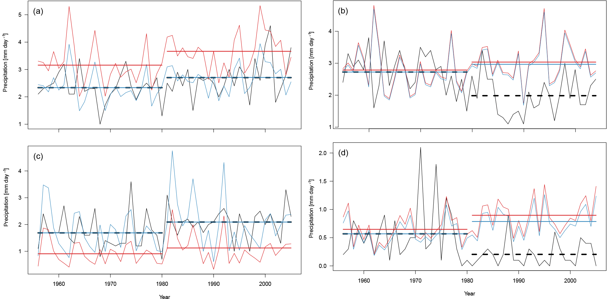
Figure 2 Time series of boreal summer (JJA) precipitation. (a) case 1 (true negative); (a) case 2 (false positive); (c) case 3 (false negative); (d) case 4 (true negative). Black: E-OBS; red: raw EC-EARTH; blue: bias-corrected EC-EARTH. The straight horizontal lines depict the long-term means over calibration and validation periods, respectively.

Download

Figure 2 shows observed and simulated time series, the latter before and after bias correction, for the four cases we considered. Figure 2a and b show the sensible examples, Fig. 2c and d the non-sensible examples. In Fig. 2a and c, observed and simulated trends randomly agree, and in Fig. 2b and d they randomly disagree. As shown analytically in Sect. 3, the residual bias vanishes in cases (a) and (c), where the relative trends in observations and simulations are similar, and it does not vanish in (b) and (d), where the relative trends in observations and simulations disagree. The relevant cases are (b) and (c): in the former, the bias correction is in principle sensible, but the holdout method would suggest that it was not sensible (false positive). In the latter, the bias correction is not sensible, but the holdout method would suggest that it was sensible (false negative). These examples clearly illustrate our previous reasoning: the holdout method, and thus also cross-validation, yields misleading results when it is used to assess the sensibility of bias-corrected climate change simulations against observations.

E-OBS data are available from the ECA&D website at https://www.ecad.eu/ (last access: 21 July 2017). EC-EARTH data are available from the ESGF nodes accessible via https://esgf.llnl.gov/nodes.html (last access: 17 September 2018).

DM and MW developed the idea for the study. DM conducted the analytical derivations, carried out the analysis, and wrote the manuscript. MW commented on the manuscript. DM and MW discussed the results.

The authors declare that they have no conflict of interest.