the Creative Commons Attribution 4.0 License.
the Creative Commons Attribution 4.0 License.
 | 02 Oct 2018
Rainfall-runoff modelling using river-stage time series in the absence of reliable discharge information: a case study in the semi-arid Mara River basin
Petra Hulsman
Thom A. Bogaard
Hubert H. G. Savenije
Hydrological models play an important role in water resources management. These models generally rely on discharge data for calibration. Discharge time series are normally derived from observed water levels by using a rating curve. However, this method suffers from many uncertainties due to insufficient observations, inadequate rating curve fitting procedures, rating curve extrapolation, and temporal changes in the river geometry. Unfortunately, this problem is prominent in many African river basins. In this study, an alternative calibration method is presented using water-level time series instead of discharge, applied to a semi-distributed rainfall-runoff model for the semi-arid and poorly gauged Mara River basin in Kenya. The modelled discharges were converted into water levels using the Strickler–Manning formula. This method produces an additional model output; this is a “geometric rating curve equation” that relates the modelled discharge to the observed water level using the Strickler–Manning formula and a calibrated slope-roughness parameter. This procedure resulted in good and consistent model results during calibration and validation. The hydrological model was able to reproduce the water levels for the entire basin as well as for the Nyangores sub-catchment in the north. The newly derived geometric rating curves were subsequently compared to the existing rating curves. At the catchment outlet of the Mara, these differed significantly, most likely due to uncertainties in the recorded discharge time series. However, at the “Nyangores” sub-catchment, the geometric and recorded discharge were almost identical. In conclusion, the results obtained for the Mara River basin illustrate that with the proposed calibration method, the water-level time series can be simulated well, and that the discharge-water-level relation can also be derived, even in catchments with uncertain or lacking rating curve information.
Please read the corrigendum first before continuing.
-
Notice on corrigendum
The requested paper has a corresponding corrigendum published. Please read the corrigendum first before downloading the article.
-
Article
(5459 KB)
- Corrigendum
-
Supplement
(2299 KB)
-
The requested paper has a corresponding corrigendum published. Please read the corrigendum first before downloading the article.
- Article
(5459 KB) - Corrigendum
-
Supplement
(2299 KB) - BibTeX
- EndNote


Hydrological models play an important role in water resources management. In hydrological modelling, discharge time series are of crucial importance. For example, discharge is used when estimating flood peaks (Di Baldassarre et al., 2012; Kuczera, 1996), calibrating models (Domeneghetti et al., 2012; McMillan et al., 2010) or determining the model structure (McMillan and Westerberg, 2015; Bulygina and Gupta, 2011). Discharge is commonly measured indirectly through the interpolation of velocity measurements over the cross-section (WMO, 2008; Di Baldassarre and Montanari, 2009). However, to obtain frequent or continuous discharge data, this method is time consuming and cost-inefficient. Moreover, in African river catchments, the quantity and quality of the available discharge measurements are often unfortunately inadequate for the reliable calibration of hydrological models (Shahin, 2002; Hrachowitz et al., 2013).
There are several sources of uncertainty in discharge data when using rating curves that cannot be neglected. First, measurement errors in the individual discharge measurements affect the estimated continuous discharge data, for example in the velocity-area method, uncertainties in the cross-section and velocity can arise due to poor sampling (Pelletier, 1988; Sikorska et al., 2013). Second, these measurements are usually conducted during normal flows. However during floods, the rating curve needs to be extrapolated. Therefore, the uncertainty increases for discharges under extreme conditions (Di Baldassarre and Claps, 2011; Domeneghetti et al., 2012). Thirdly, the fitting procedure does not always account well for irregularities in the profile, particularly when banks are overtopped. Finally, the river is a dynamic, non-stationary system which influences the rating curve, for example changes in the cross-section due to sedimentation or erosion, backwater effects or hysteresis (Petersen-Øverleir, 2006). The lack of incorporating such temporal changes in the rating curve increases the uncertainty in discharge data (Guerrero et al., 2012; Jalbert et al., 2011; Morlot et al., 2014). As a result, the rating curve should be regularly updated to take such changes into account. The timing of adjusting the rating curve relative to the changes in the river affects the number of rating curves and the uncertainty (Tomkins, 2014). Previous studies focused on assessing the uncertainty of rating curves (Di Baldassarre and Montanari, 2009; Clarke, 1999) and their effect on model predictions (Karamuz et al., 2016; Sellami et al., 2013; Thyer et al., 2011).
In the absence of reliable rating curves, remotely sensed river characteristics related to the discharge such as river width and water level can provide valuable information on the flow dynamics for model calibration and validation. For instance, previous studies derived the discharge from remotely sensed river width (Revilla-Romero et al., 2015; Yan et al., 2015; Sun et al., 2015) or river water levels measured with radar altimetry (Pereira-Cardenal et al., 2011; Michailovsky et al., 2012; Ričko et al., 2012; Schwatke et al., 2015; Tourian et al., 2017; Sun et al., 2012). In previous studies, hydrological models were calibrated on river width or surface water extent (Sun et al., 2015; Revilla-Romero et al., 2015). Also radar altimetry observations of river water levels have been used to calibrate or validate hydrological models by using empirical equations transforming discharge to the water level without using cross-section information (Sun et al., 2012; Getirana, 2010), for instance conceptual hydrological models (Sun et al., 2012; Pereira-Cardenal et al., 2011) or process-based models (Getirana, 2010; Paiva et al., 2013).
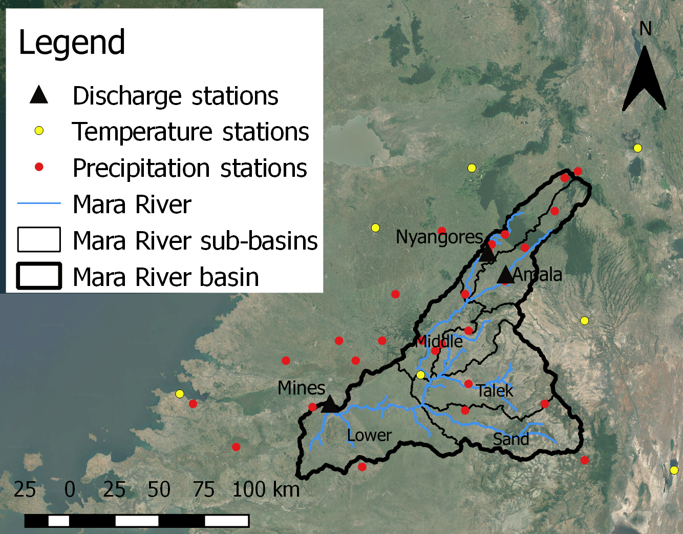
Figure 1Map of the Mara River basin and the hydro-meteorological stations for which data are available.
Besides remotely sensed river characteristics, locally measured river water-level time series are also valuable for model calibration and validation (van Meerveld et al., 2017). In general, water-level time series are more reliable than discharge data or remotely sensed river characteristics, as these are direct measurements and not processed data. In previous studies, hydrological models have been calibrated on river water-level time series using the Spearman rank correlation coefficient (Jian et al., 2017; Seibert and Vis, 2016) or by including an inverse rating curve with three new calibration parameters to convert the modelled discharge to water level (Jian et al., 2017). When using the Spearman rank correlation function, the focus is on correlating the ranks instead of the magnitudes, which as a result, introduces biases in the model results. Alternatively, rainfall-runoff models can be calibrated on water-level time series combined with a hydraulic equation introducing only one new calibration parameter. Data-driven models have also been calibrated successfully on water-level time series; for example artificial neural network or fuzzy logic approaches were applied (Liu and Chung, 2014; Panda et al., 2010; Alvisi et al., 2006).
The goal of this study is to illustrate the potential of water-level time series for hydrological model calibration by incorporating a hydraulic equation describing the rating curve within the model. This calibration method is applied to the semi-arid and poorly gauged Mara River basin in Kenya. For three gauging stations within this basin, the quality of the recorded rating curves have been analysed and compared to the model results. For this purpose, a semi-distributed rainfall-runoff model has been developed on a daily timescale applying the FLEX-Topo modelling concept (Savenije, 2010).
The Mara River originates in Kenya in the Mau Escarpment and flows through the Maasai Mara National Reserve in Kenya into Lake Victoria in Tanzania. The main tributaries are the Nyangores and Amala rivers in the upper reach and the Lemek, Talak and Sand in the middle reach (Fig. 1). The first two tributaries are perennial, while the remaining tributaries are ephemeral, which generally dry out during dry periods. In total, the river is 395 km long (Dessu et al., 2014) and its catchment covers an area of about 11 500 km2 (McClain et al., 2013), of which 65 % is located in Kenya (Mati et al., 2008).
Table 1Hydro-meteorological data availability in the Mara River basin. The temporal coverage for water level and discharge can be different due to poor administration.
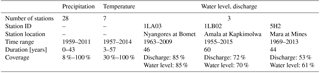
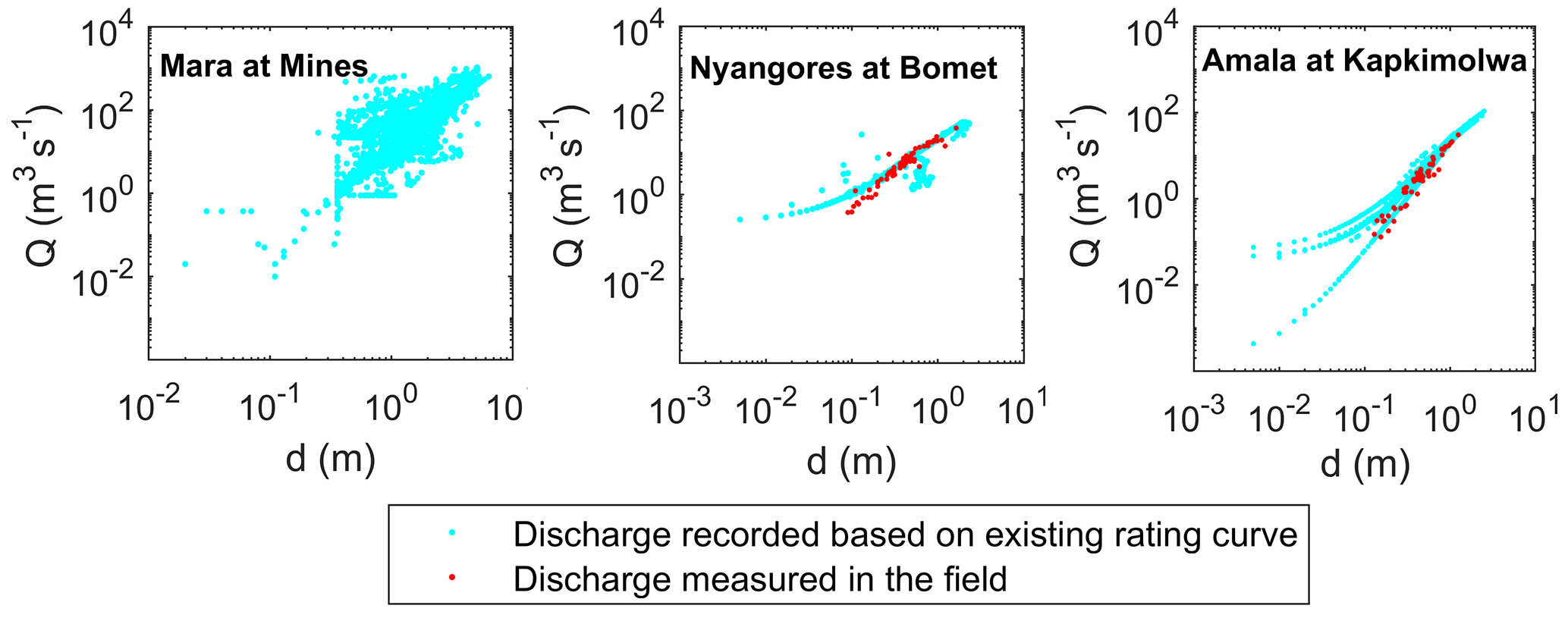
Figure 2Discharge–water depth graphs for the three main river gauging stations in the Mara River basin; these are the Mara at Mines, Nyangores at Bomet and Amala at Kapkimolwa. For each location, the following are visualised: (1) recorded discharge and water-level time series between 1960 and 2010 (light blue), (2) discharge field measurements from the Nile Decision Support Tool (NDST) for the time period 1963–1989 (Nyangores) and 1965–1992 (Amala); no data were available for Mines (red).
Within the Mara River basin, there are two wet seasons linked to the annual oscillations of the ITCZ (Intertropical Convergence Zone). The first wet season is from March to May and the second from October to December (McClain et al., 2013). The precipitation varies spatially over the catchment following the local topography. The largest annual rainfall can be found in the upstream area of the catchment, which is between 1000 and 1750 mm yr−1. In the middle and downstream areas, the annual rainfall is between 900 and 1000 mm yr−1 and between 300 and 850 mm yr−1, respectively (Dessu et al., 2014).
The elevation of the river basin varies between 3000 m a.s.l. (metres above sea level) at the Mau Escarpment, 1480 m at the border to Tanzania and 1130 m at Lake Victoria (McClain et al., 2013). In the Mara River basin, the main land cover types are agriculture, grass, shrubs and forests. The main forest in the catchment is the Mau forest, which is located in the north. Croplands are mainly found in the north and in the south, whereas the middle part is dominated by grasslands.
2.1 Data availability
2.1.1 In situ monitoring data
In the Mara River basin, long-term daily water level and discharge time series are available for 44–60 years between 1955 and 2015 at the downstream station near Mines and in the two main tributaries, the Nyangores and Amala. In addition, precipitation and air temperature is measured at 27 and 7 stations, respectively (Fig. 1 and Table 1). However, the temporal coverage of these data are poor, as there are many gaps.
There are many uncertainties in the discharge and precipitation data in the Mara River basin. Discharge data analyses indicated that the time series were unreliable due to various inconsistencies in the data, especially at Mines and Amala. At Mines, a high scatter in the discharge-water-level graph was observed (Fig. 2) and back-calculated cross-section average flow velocities were below 1 m s−1 (Fig. S1 in the Supplement), whereas in 2012 the measured velocity was 2.13 m s−1 and the discharge 529.3 m3 s−1 (GLOWS-FIU, 2012). At Amala, the rating curves were adjusted multiple times, affecting mostly the low flows. Only the rating curve at Nyangores was stable and consistent with field measurements. The precipitation data analysis showed a high spatial variability between the limited number of rainfall stations available. More information can be found in “S1 Data quality” in the Supplement.
Table 2Discharge measured in the field using an Acoustic Doppler Profiler (SonTek RiverSurveyor M9) mounted on a portable raft that is also equipped with a Power Communications Module and a DGPS (Rey et al., 2015).
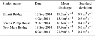
During field trips, point discharge measurements were done in September and October 2014 at Emarti Bridge, Serena Pump House and New Mara Bridge (see Table 2 and Fig. 3). At each location, the discharge was derived using an Acoustic Doppler Profiler (SonTek RiverSurveyor M9) mounted on a portable raft that is also equipped with a Power Communications Module and a Differential Global Positioning System (DGPS) antenna (Rey et al., 2015).
2.1.2 Remotely sensed data
Besides ground observations, remotely sensed data were also used for setting up the rainfall-runoff model. Catchment classification was based on topography and land cover. For the topography, a digital elevation map (SRTM) with a resolution of 90 m and vertical accuracy of 16 m was used (US Geological Survey, 2014). The land cover was based on Africover, a land cover database based on ground truth and satellite images (FAO-UN, 2002). For the climate, remotely sensed precipitation was used from the Famine Early Warning Systems Network (FEWS NET) on a daily timescale from 2001 to 2010 and monthly actual evaporation from USGS from 2001 to 2013. Moreover, normalised difference vegetation index (NDVI) maps derived from Landsat images were used to define parameter constraints.
3.1 Catchment classification based on landscape and land use
For this study, the modelling concept of FLEX-Topo has been used (Savenije, 2010). It is a semi-distributed rainfall-runoff modelling framework that distinguishes hydrological response units (HRUs) based on landscape features. The landscape classes were identified based on the topographical indices HAND (Height Above Nearest Drain) and slope using a digital elevation map. Hillslopes are defined by a strong slope and high HAND, wetlands by a low HAND, and terraces by a high HAND and mild slope. The threshold for the slope (21.9 %) was based on a sensitivity analyses within the Mara basin, which revealed that the area of hillslopes changed asymptotically with the threshold. Therefore, the slope threshold was chosen at the point where changes in the sloped area become insignificant. As the wetland area was insignificant based on field observations, the HAND threshold was set to zero. In the Mara River basin, there are mainly terraces and hillslopes.
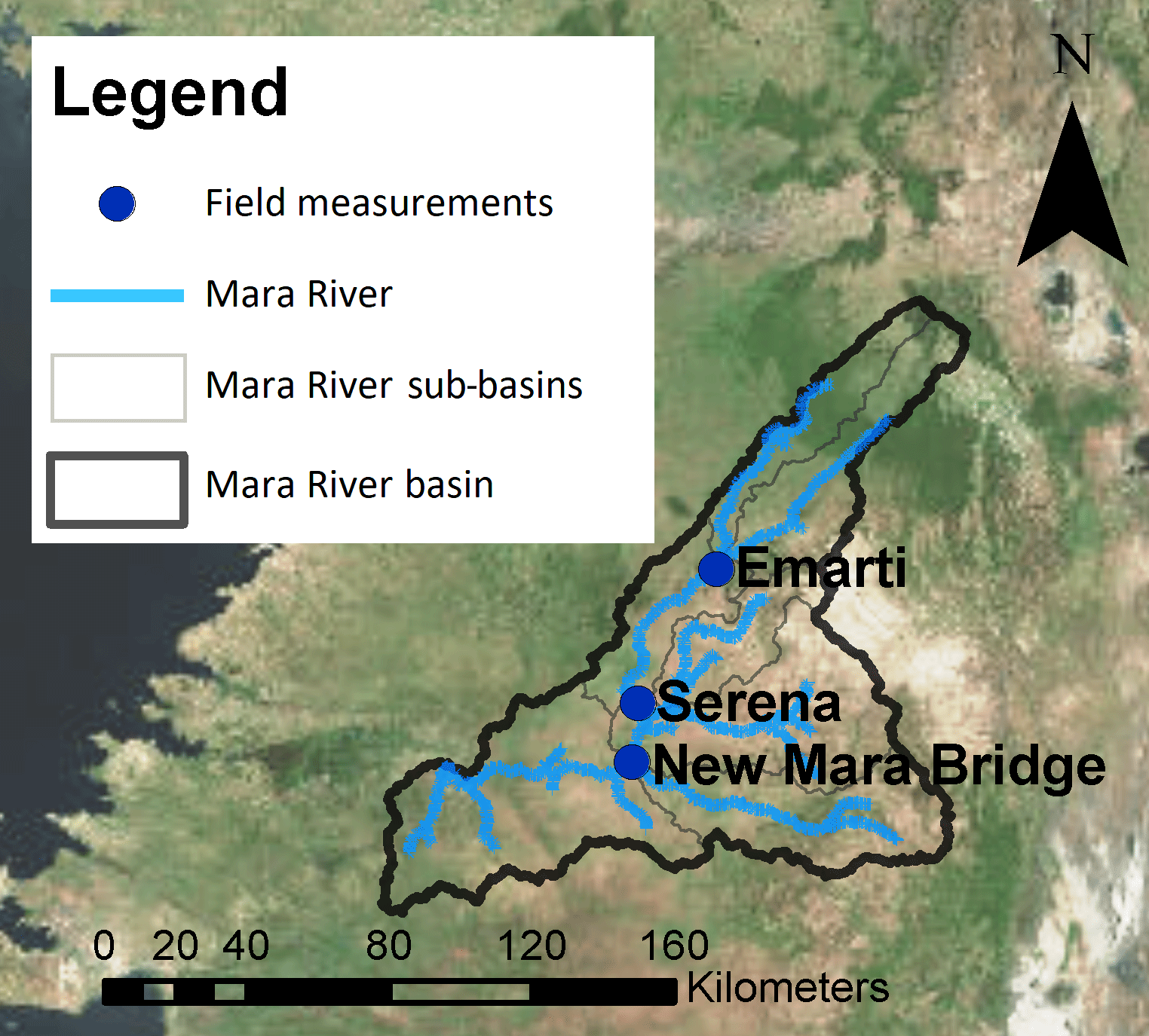
Figure 3Map of discharge measurement locations during field trips in September and October 2014.
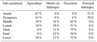
To further delimit these two main landscape units, the land cover is taken into account as well. In the upper sub-catchments, there are mainly croplands and forests, whereas further south, the land use is dominated by grasslands. In the lower sub-catchment, there are mostly croplands and grasslands. This resulted in four HRUs within the sub-basin of the Mara River basin, namely forested hillslopes, shrubs on hillslopes, agriculture and grassland (Figs. 4 and 5 and Table 3).
3.2 Hydrological model structure
Each HRU is represented by a lumped conceptual model; the model structure is based on the dominant flow processes observed during field trips or deducted from interviews with local people. For example, in forests and shrub lands, shallow subsurface flow (SSF) was seen to be the dominating flow mechanism; rainwater infiltrates into the soil and flows through preferential flow paths to the river. In contrast, grassland and cropland generate overland flow. The observed soil compaction, due to cattle trampling and ploughing, reduces the preferential infiltration capacity resulting in overland flow during heavy rainfall. Consequently, the Hortonian overland flow (HOF) occurs at high rainfall intensities exceeding the maximum infiltration capacity. The perception of the dominant flow mechanisms (Fig. 5) was then used to develop the model structure (Fig. 6). This approach of translating a perceptual model into a model concept (Beven, 2012) was applied successfully in previous FLEX-Topo applications (Gao et al., 2014a; Gharari et al., 2014).
Table 3Classification results, namely the area percentage of each hydrological response unit per sub-catchment in the Mara River basin.
The model structure contains multiple storage components schematised as reservoirs (Fig. 6). For each reservoir, the inflow, outflow and storage are defined by water balance equations, see Table 4. Process equations determine the fluxes between these reservoirs as a function of input drivers and their storage. HRUs function in parallel and independently from each other. However, they are connected to the groundwater system and the drainage network. To find the total runoff at the sub-catchment outlet Qm,sub, the outflow Qm,i of each HRU is multiplied by its relative area and then added up together with the groundwater discharge Qs. The relative area is the area of a specific HRU divided by the entire sub-catchment area. Subsequently, the modelled discharge at the catchment outlet is obtained by using a simple river routing technique, where a delay from sub-catchment outlet to catchment outlet was added assuming an average river flow velocity of 0.5 m s−1. In the Sand sub-catchment, it is schematised that runoff can percolate to the groundwater from the riverbed and that moisture can evaporate from the groundwater through deep rooting or riparian vegetation.
3.3 Model constraints
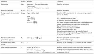
Parameters and process constraints were applied to eliminate unrealistic parameter combinations and constrain the flow volume. Parameter constraints were applied to the maximum interception, reservoir coefficients, the storage capacity in the root zone or on the surface, and the slope-roughness parameter, Table 5. Process constraints were applied to the runoff coefficient, groundwater recharge, interception and infiltration, Table 6. The effect of including these parameter and process constraints is illustrated in Fig. S5. For instance, the maximum storage in the unsaturated zone Su,max equals the root zone storage capacity and was estimated using the method of Gao et al. (2014b) based on remotely sensed precipitation and evaporation (Gao et al., 2014b; Wang-Erlandsson et al., 2016). The dry season evaporation has been derived from the actual evaporation using the NDVI.
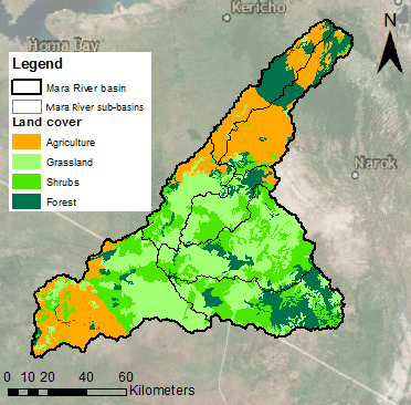
Figure 4Classification of the Mara River basin into four hydrological response units for each sub-catchment based on land use and landscape.
Table 4Equations applied in the hydrological model. The formulas for the unsaturated zone are written for the hydrological response units, namely forested hillslopes and shrubs on hillslopes; for grass and agriculture, the inflow Pe changes to QF. The modelling time step is Δt=1 day. Note that at a time daily step, the transfer of interception storage between consecutive days is assumed to be negligible.
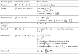
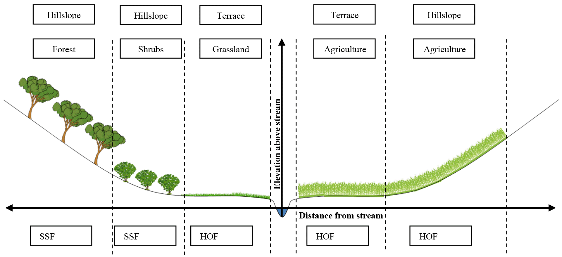
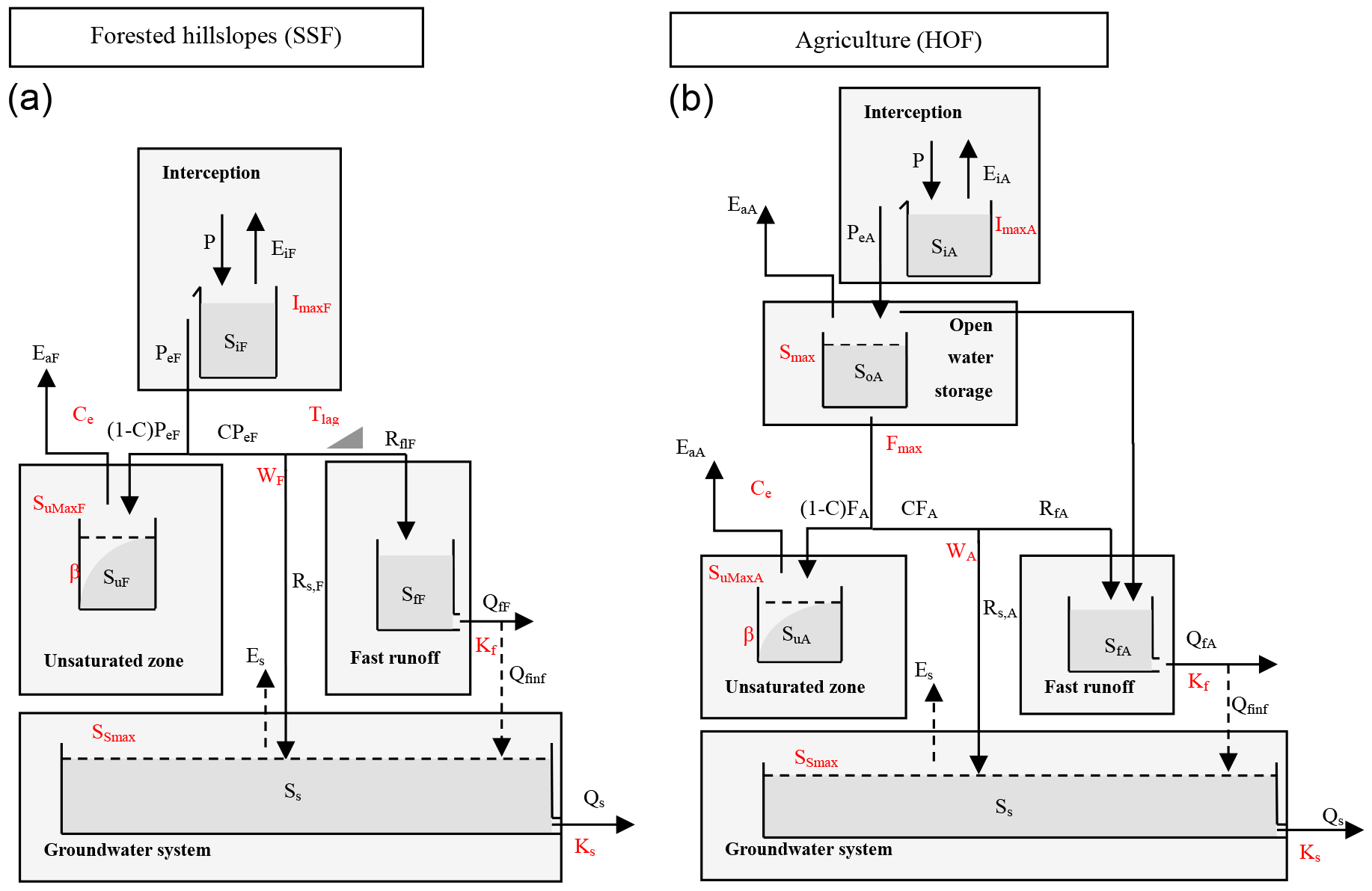
Figure 6Model structure of the HRUs for forested hillslopes (a) and agriculture (b). The structure for shrubs on hillslopes is similar to the left one, replacing the indices F with S. The structure for grassland is similar to the right one, replacing the indices A with G. Parameters are marked in red and storages and fluxes in black. In terms of the symbol explanation for fluxes, precipitation is denoted by (P), evaporation of the interception zone by (Ei), actual evaporation by (Ea), evaporation from groundwater only applied in the sub-catchment Sand by (Es), effective precipitation by (Pe), infiltration into the unsaturated zone by (F), discharge from unsaturated zone to the fast runoff zone by (Rf), groundwater recharge by (Rs), discharge from the fast runoff by (Qf), infiltration into groundwater system only applied in the sub-catchment Sand by (Qf,inf) and discharge from the slow runoff by (Qs). For storages, storage in the interception zone is denoted by (Si), open water storage by (So), storage in the root zone by (Su), storage for the slow runoff by (Ss), storage for the fast runoff by (Sf). For the remaining symbols, splitter is denoted by (W) and (C), the soil moisture distribution coefficient by (β), the transpiration coefficient by (Ce=0.5), and the reservoir coefficient by (K); indices f and s indicate the fast and slow runoff. Units used are for fluxes [mm day−1], storages [mm], reservoir coefficient [day] and remaining parameters [–].
3.4 Model calibration method using water levels
The hydrological model was calibrated on a daily timescale applying the MOSCEM-UA algorithm (Vrugt et al., 2003), with parameter ranges and values as indicated in Tables S1 and S2 in the Supplement. For the calibration, the Nash–Sutcliffe coefficient (Nash and Sutcliffe, 1970) was applied to the water-level duration curve (Eq. 1 linear, and Eq. 2 log-scale). This frequently used objective function is advantageous, as it is sensitive not only to high flows, but also to low flows when using logarithmic values (Krause et al., 2005; McCuen Richard et al., 2006; Pushpalatha et al., 2012). By calibrating on the duration curve, the focus is on the flow statistics and not on the timing of individual flow peaks. This information is also in the time series. This is justified, since there were high uncertainties in the timings of floods events due to the limited number of available rainfall stations to capture the spatial variability of the rainfall input well. Therefore, duration curves were considered as a good signature for calibrating this model; this was also concluded in previous studies (Westerberg et al., 2011; Yadav et al., 2007). This signature was incorporated in the objective functions with the following equations:
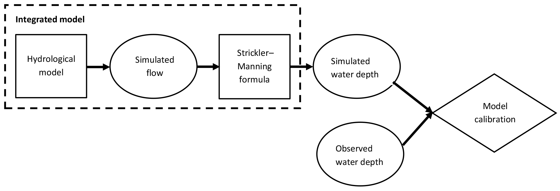
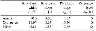
For the water-level-based calibration, the modelled discharge needs to be converted to the modelled water level. This calculation was done with the Strickler–Manning formula, in which the discharge is a function of the water level (Eq. 3) and where R is the hydraulic radius (Eq. 6), A the cross-sectional area (Eq. 5), i the slope, k the roughness and c the slope-roughness parameter (Eq. 4). The hydraulic radius and cross-section are a function of the water depth d, which is the water level subtracted h by the reference level h0 (Eq. 7). The cross-sections were simplified as a trapezium with river width B and two different riverbank slopes i1 and i2; these coefficients (Table 7) were estimated based on the available cross-section information (Figs. S6–S8). Since the slope and roughness are unknown, the slope-roughness parameter c was calibrated. The following equations were applied for these calculations:
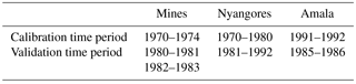
This model calibration method, illustrated graphically in Fig. 7, was applied to three basins individually, namely to the entire river basin using the station Mines and for the sub-catchments Nyangores and Amala. At each location, the model was calibrated and validated for time periods indicated in Table 8; at Mines, two time periods were used for validation to maximise the use of the available ground measurements.
Table 5Overview of all parameter constraints applied in the hydrological model for the Mara River basin.
3.5 Rating curve analysis
After calibration, the modelled water levels and discharges were analysed. For the model calibration and validation, the modelled and recorded water levels were compared at the basin level, focusing on the time series and the duration curves. Hereafter, water-level–discharge relations were analysed taking two rating curves into consideration:
-
The “recorded rating curve” relates Qrec to hobs.
-
The “geometric rating curve” relates QStrickler to hobs.
The geometric rating curve relates the modelled discharge QStrickler to the observed water level hobs. This discharge QStrickler was calculated with the Strickler–Manning formula using the calibrated slope-roughness parameter c, cross-section data, and the observed water level hobs. Therefore, the equation behind the geometric rating curve is basically the Strickler–Manning formula (Eq. 3) instead of the traditional rating curve equation (Eq. 8). The advantage of the Strickler–Manning formula is that only one parameter is unknown (riverbed slope and roughness c, Eq. 4), instead of two (fitting parameters a and b). However, the Strickler–Manning rating curve approach requires additional information on the cross-section. This is represented by
Table 6Overview of all process constraints applied in the hydrological model for the Mara River basin.
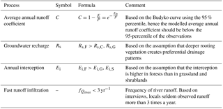
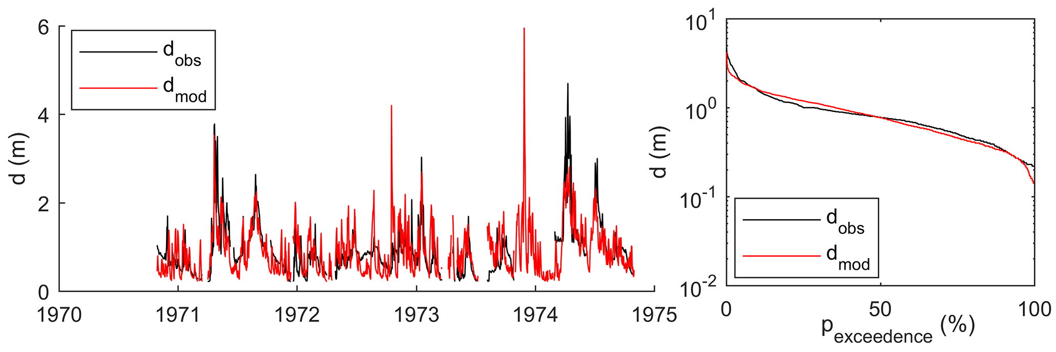
Figure 8Model results at Mines during calibration for water depth time series and water depth exceedance.
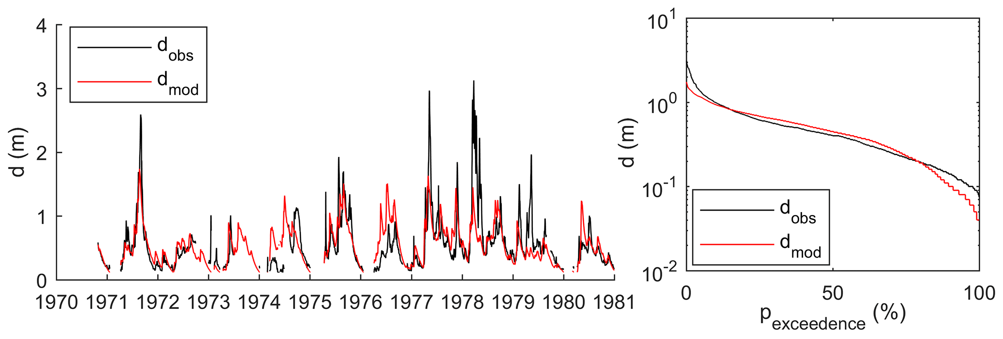
Figure 9Model results at Nyangores during calibration for water depth time series and water depth exceedance.
4.1 Water-level time series and duration curve
Model results were analysed graphically (Figs. 8 to 10 and Figs. S9 to S19) and numerically based on the Nash–Sutcliffe values for the objective functions (Table 9). The results of the objective functions indicate that at Nyangores and Mines, the calibration and validation results were consistent. At Mines, the modelled water level was simulated well, particularly with regard to the duration curve (Fig. 8). At individual events, there were substantial differences. In some years, for example in 1974, the observed data were very well represented by the model outcome. However, in other years this was not the case. In general, the model captured the dynamics in the water level well. This was the case during both calibration and validation (see Figs. S12 and S13).
At Nyangores the observed and modelled water levels were also similar during calibration and validation, extremely high flows excluded (Fig. 9). However, at Amala, the observed and modelled water levels differed significantly during calibration (Fig. 10) and validation (Fig. S15). The model missed several discharge events completely, likely related to missing rainfall events in the input data due to the high heterogeneity in precipitation.
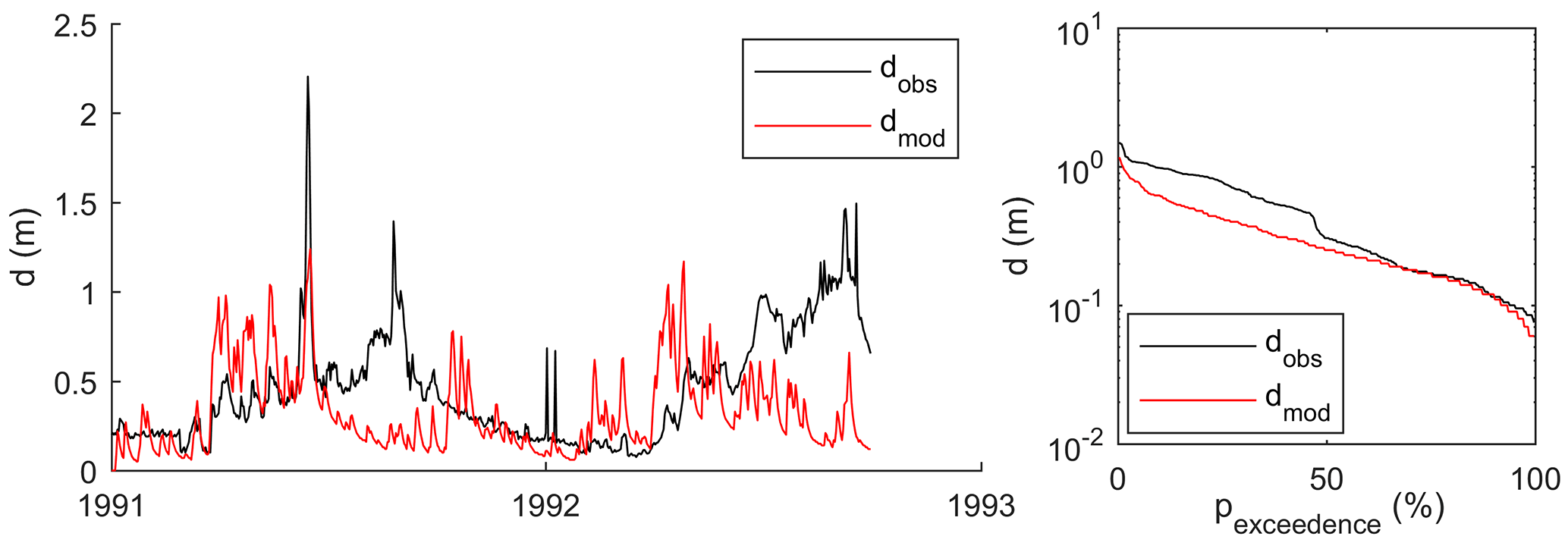
Figure 10Model results at Amala during calibration for water depth time series and water depth exceedance.
4.2 Discharge at sub-catchment level
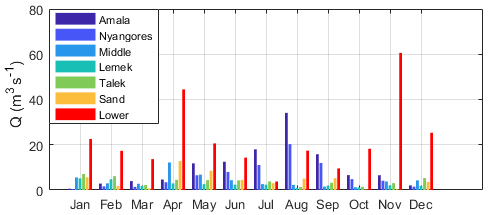
At Mines, the discharge originates from seven different sub-catchments, each with a different contribution. Based on field observations, the mountainous upstream sub-catchments from the north should have the largest contribution, whereas the contribution from the relatively drier and flatter Lemek and Talek tributaries from the eastern part of the catchment should be relatively low. The contribution of each sub-catchment to the total modelled discharge was assessed on a monthly timescale and compared with observations.
As shown in Fig. 11, the contribution varied throughout the year. In the summer (July–September), the modelled discharge mainly originates from the northern sub-catchments, Nyangores and Amala. However, in the winter (November–April), the modelled discharge mainly originates from the Sand and Lower sub-catchments. The eastern Middle, Talek and Lemek sub-catchments have the lowest discharge throughout the entire year, as has been similarly observed.
Table 8Time periods used for the calibration and validation at the three basins of Mines, Nyangores and Amala.
In previous studies, it has been shown that only a few discharge measurements can contain sufficient information to constrain model predictive uncertainties effectively (Seibert and Beven, 2009). To evaluate the model at the sub-catchment level, model results were compared with discharge measurements done during field trips in September and October 2014 at the Emarti Bridge, Serena Pump House and New Mara Bridge. At all three locations, the point measurements fitted well within the range of the modelled discharge (see Fig. 12).
Table 9Overview of the values of the objective functions for each model simulation. Calibration was done based on the water level using NSlog (h) and NSh; for comparison, objective functions using the discharge were added here as well.
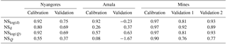
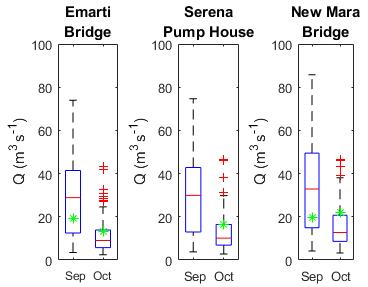
Figure 12Box plot of the modelled discharge at three locations; the green asterisk represents the measured discharge in September and October 2014.
4.3 Rating curve analysis
In this study, the recorded and geometric (Strickler–Manning) rating curves were compared (Fig. 13). At Mines, these two rating curves differed significantly. On the one hand, for medium to high flows, both the recorded and geometric rating curves run parallel, indicating similar cross-sectional properties; only the offset differed through changing riverbed levels. On the other hand, the simulated cross-section average flow velocities were realistic compared to the point measurements at Mines indicating that velocities are greater than 2 m s−1 during high flows (see Fig. 13). At Nyangores, the recorded and geometric rating curves were almost identical, while there were significant differences at the Amala gauging station, especially in the low flows. Interestingly, these observations also hold for the validation period for all three stations.
The difference between the recorded and geometric rating curves at Mines probably resulted from uncertainties in the available recorded discharge data. In the complete discharge–water-level graphs for all available data (Fig. S2), large scatter was found. This could be the result of natural variability in the reference water level h0 in the rating curve equation, which was not taken into account. A sensitivity analysis of the recorded rating curve equation at Mines showed that a deviation of 0.1 m in the reference water level could alter the discharge with 4 % for high flows and 46 % for low flows. However, a deviation of 0.5 m resulted in a 19 %–325 % change in the discharge. Therefore, unnoticed variations in the riverbed level strongly affect the uncertainty in the recorded rating curve at Mara Mines, which is located in a morphologically dynamic section of the river (Stoop, 2017).
At Amala, the difference between both rating curves could be related to the effect of missing rain events in the input data as result of the short time series for calibration and validation. This resulted in absent discharge peaks and hence an underestimation of the flow; these were the most extreme at Amala. During model calibration, this was compensated by increasing the parameter c in the Strickler–Manning formula (Eq. 4). As a result, discharge values not only increased during missed events, but also for all other days. The compensation effect was limited though, since the model was calibrated on the duration curves instead of the time series. As parameter c is linearly related to the geometric rating curve (Eq. 3), the latter was overestimated as well. Therefore, missing rain events in the input data resulted in the overestimation of the geometric rating curve.
In short, at the two stations with inconsistent rating curves, Amala and Mines, the geometric rating curve deviated significantly from the recordings. Strikingly, the deviations were observed at the same flow magnitudes where large inconsistencies were found in the observations, for instance in the low flows at Amala. However, at the gauging station with a reliable rating curve, Nyangores, the geometric and recorded discharge–water-level relations were almost identical.

Figure 13Model calibration results at Mines, Nyangores and Amala for discharge–water depth graphs (a) and velocity–water depth graphs (b).
4.4 Limitations
This paper illustrated that the proposed water-level calibration method simulated the discharge-water-level relation well for the gauging station where consistent rating curve information was available. However, there are several limitations to this method. First, the slope-roughness parameter compensates for non-closure effects in the water balance, for instance due to errors in the precipitation, which is extremely heterogeneous in the semi-arid Mara basin. Unfortunately, this heterogeneity is poorly described in our study area with the available rain gauges (see Sect. S7.2 on the precipitation data analysis), influencing the modelling results. Therefore, this parameter should be constrained to minimise this compensation as much as possible. Second, the cross-section was assumed to be constant during the modelling time period. Data analyses indicated that expected changes in the river width or slope cannot affect the rating curve significantly. However, if this is not the case, then this cross-section change should be included during the model calibration.
In previous studies, river water-level time series were used for model calibration by using the Spearman rank correlation function (Seibert and Vis, 2016) or an inverse rating curve to convert the modelled discharge to water level (Jian et al., 2017). Compared to these approaches, the calibration method proposed in this paper has the following advantages: (1) Water-level time series are direct measurements and are therefore more reliable compared to processed data such as satellite based measurements. (2) Merely one new calibration parameter (the slope-roughness parameter) is introduced instead of three when using an inverse rating curve. (3) The model is calibrated on water-level magnitudes instead of only the ranks, which would introduce biases. However, this method also has several disadvantages; (1) cross-section information is needed and is assumed to be constant over the time period for which it is applied and (2) the newly introduced slope-roughness parameter compensates for non-closure effects in the water balance when not constrained well.
The goal of this paper was to illustrate a new calibration method using water-level time series and the Strickler–Manning formula instead of discharge in a semi-arid and poorly gauged basin. This method offers a potential alternative for calibration on discharge data, as is also common practice in poorly gauged catchments. The semi-distributed rainfall-runoff modelling framework FLEX-Topo was applied. The catchment was divided into four hydrological response units (HRUs) and seven sub-catchments based on the river tributaries. For each HRU, a unique model structure was defined based on the observed dominant flow processes. By constraining the parameters and processes, unrealistic parameter sets were excluded from the calibration parameter set and the flow volume was constrained. This model was calibrated based on water levels to capture the flow dynamics. For this purpose, the modelled discharge was converted to water levels using the Strickler–Manning formula. The unknown slope-roughness parameter was calibrated.
An important output of this calibration approach is the “geometric rating curve equation”, which relates the discharge to the water level using the Strickler–Manning formula. The geometric and recorded rating curves were significantly different at two gauging stations, namely Mines, the catchment outlet, and Amala, a sub-catchment outlet. At both locations, the deviations were at the same flow magnitudes where large inconsistencies were found in the observations. However, at the gauging station with a reliable rating curve, Nyangores, the recorded and geometric discharge-water-level relations were almost identical. In conclusion, this calibration method allows reliable simulations of the discharge–water-level relation, even in a data-poor region.
In addition, this paper analysed the current status of the hydro-meteorological network in the Mara River basin, focusing on the data availability and quality. Moreover, a hydrological model and an improved geometric rating curve equation were developed for this river. All three aspects contribute to improving the assessment of the water resources availability in the Mara River basin.
For future studies, it would be interesting to apply this calibration method to other studies of river basins with different climatic conditions and better data availability. Furthermore, it is recommended to assess the effect of rainfall uncertainties on this calibration method. Moreover, the hydrological model was calibrated on two signatures and two objective functions only. However, whether these signatures and objective functions provide sufficient information for calibration has not been analysed. Therefore, the procedures for water-level-based calibration should be analysed in more detail.
Station data (discharge, water level and precipitation) was provided by the Water Resource Management Authority (WRMA) in Kenya. Temperature and additional precipitation data was obtained from the NOAA online database (Menne et al., 2012). More detailed information can be found in Sect. 2.1.
The supplement related to this article is available online at: https://doi.org/10.5194/hess-22-5081-2018-supplement.
This paper has been co-authored by TAB and HHGS. Their contribution and support to this research has been valued very much.
The authors declare that they have no conflict of interest.
This research was part of the MaMaSe project (Mau Mara Serengeti) led by IHE Delft.
Edited by: Elena Toth
Reviewed by: two anonymous referees
Alvisi, S., Mascellani, G., Franchini, M., and Bárdossy, A.: Water level forecasting through fuzzy logic and artificial neural network approaches, Hydrol. Earth Syst. Sci., 10, 1–17, https://doi.org/10.5194/hess-10-1-2006, 2006.
Beven, K. J.: Rainfall-runoff modelling: the primer, John Wiley & Sons, Chichester, England, https://doi.org/10.1002/9781119951001, 2012.
Bulygina, N. and Gupta, H.: Correcting the mathematical structure of a hydrological model via Bayesian data assimilation, Water Resour. Res., 47, https://doi.org/10.1029/2010WR009614, 2011.
Clarke, R. T.: Uncertainty in the estimation of mean annual flood due to rating-curve indefinition, J. Hydrol., 222, 185–190, https://doi.org/10.1016/S0022-1694(99)00097-9, 1999.
Dessu, S. B., Melesse, A. M., Bhat, M. G., and McClain, M. E.: Assessment of water resources availability and demand in the Mara River Basin, Catena, 115, 104–114, https://doi.org/10.1016/j.catena.2013.11.017, 2014.
Di Baldassarre, G. and Claps, P.: A hydraulic study on the applicability of flood rating curves, Hydrol. Res., 42, 10–19, https://doi.org/10.2166/nh.2010.098, 2011.
Di Baldassarre, G. and Montanari, A.: Uncertainty in river discharge observations: a quantitative analysis, Hydrol. Earth Syst. Sci., 13, 913–921, https://doi.org/10.5194/hess-13-913-2009, 2009.
Di Baldassarre, G., Laio, F., and Montanari, A.: Effect of observation errors on the uncertainty of design floods, Phys. Chem. Earth Pt. A/B/C, 42–44, 85–90, https://doi.org/10.1016/j.pce.2011.05.001, 2012.
Domeneghetti, A., Castellarin, A., and Brath, A.: Assessing rating-curve uncertainty and its effects on hydraulic model calibration, Hydrol. Earth Syst. Sci., 16, 1191–1202, https://doi.org/10.5194/hess-16-1191-2012, 2012.
FAO-UN: Multipurpose Landcover Database for Kenya – Africover, available at: http://www.fao.org/geonetwork/srv/en/metadata.show?id=38098&currTab=simple (last access: 27 September 2018), 2002.
Gao, H., Hrachowitz, M., Fenicia, F., Gharari, S., and Savenije, H. H. G.: Testing the realism of a topography-driven model (FLEX-Topo) in the nested catchments of the Upper Heihe, China, Hydrol. Earth Syst. Sci., 18, 1895–1915, https://doi.org/10.5194/hess-18-1895-2014, 2014a.
Gao, H., Hrachowitz, M., Schymanski, S. J., Fenicia, F., Sriwongsitanon, N., and Savenije, H. H. G.: Climate controls how ecosystems size the root zone storage capacity at catchment scale, Geophys. Res. Lett., 41, https://doi.org/10.1002/2014GL061668, 2014b.
Getirana, A. C. V.: Integrating spatial altimetry data into the automatic calibration of hydrological models, J. Hydrol., 387, 244–255, https://doi.org/10.1016/j.jhydrol.2010.04.013, 2010.
Gharari, S., Hrachowitz, M., Fenicia, F., Gao, H., and Savenije, H. H. G.: Using expert knowledge to increase realism in environmental system models can dramatically reduce the need for calibration, Hydrol. Earth Syst. Sci., 18, 4839–4859, https://doi.org/10.5194/hess-18-4839-2014, 2014.
GLOWS-FIU: Environmental Flow Recommendation for the Mara River, Kenya and Tanzania, in: Global Water for Sustainability program (GLOWS), Miami, FL, 2012.
Guerrero, J. L., Westerberg, I. K., Halldin, S., Xu, C. Y., and Lundin, L. C.: Temporal variability in stage-discharge relationships, J. Hydrol., 446–447, 90–102, https://doi.org/10.1016/j.jhydrol.2012.04.031, 2012.
Hrachowitz, M., Savenije, H. H. G., Blöschl, G., McDonnell, J. J., Sivapalan, M., Pomeroy, J. W., Arheimer, B., Blume, T., Clark, M. P., Ehret, U., Fenicia, F., Freer, J. E., Gelfan, A., Gupta, H. V., Hughes, D. A., Hut, R. W., Montanari, A., Pande, S., Tetzlaff, D., Troch, P. A., Uhlenbrook, S., Wagener, T., Winsemius, H. C., Woods, R. A., Zehe, E., and Cudennec, C.: A decade of Predictions in Ungauged Basins (PUB) – a review, Hydrolog. Sci. J., 58, 1198–1255, https://doi.org/10.1080/02626667.2013.803183, 2013.
Jalbert, J., Mathevet, T., and Favre, A. C.: Temporal uncertainty estimation of discharges from rating curves using a variographic analysis, J. Hydrol., 397, 83–92, https://doi.org/10.1016/j.jhydrol.2010.11.031, 2011.
Jian, J., Ryu, D., Costelloe, J. F., and Su, C.-H.: Towards hydrological model calibration using river level measurements, J. Hydrol.: Reg. Stud., 10, 95–109, https://doi.org/10.1016/j.ejrh.2016.12.085, 2017.
Karamuz, E., Osuch, M., and Romanowicz, R. J.: The influence of rating curve uncertainty on flow conditions in the River Vistula in Warsaw, in: Hydrodynamic and Mass Transport at Freshwater Aquatic Interfaces. GeoPlanet: Earth and Planetary Sciences, edited by: Rowiński P. and Marion A., Springer, Cham, 153–166, 2016.
Krause, P., Boyle, D. P., and Bäse, F.: Comparison of different efficiency criteria for hydrological model assessment, Adv. Geosci., 5, 89–97, https://doi.org/10.5194/adgeo-5-89-2005, 2005.
Kuczera, G.: Correlated rating curve error in flood frequency inference, Water Resour. Res., 32, 2119–2127, https://doi.org/10.1029/96WR00804, 1996.
Liu, W.-C. and Chung, C.-E.: Enhancing the Predicting Accuracy of the Water Stage Using a Physical-Based Model and an Artificial Neural Network-Genetic Algorithm in a River System, Water, 6, https://doi.org/10.3390/w6061642, 2014.
Mati, B. M., Mutie, S., Gadain, H., Home, P., and Mtalo, F.: Impacts of land-use/cover changes on the hydrology of the transboundary Mara River, Kenya/Tanzania, Lakes Reserv.: Res. Manage., 13, 169–177, 2008.
McClain, M. E., Subalusky, A. L., Anderson, E. P., Dessu, S. B., Melesse, A. M., Ndomba, P. M., Mtamba, J. O. D., Tamatamah, R. A., and Mligo, C.: Comparing flow regime, channel hydraulics and biological communities to infer flow-ecology relationships in the Mara River of Kenya and Tanzania, Hydrolog. Sci. J., 59, 1–19, https://doi.org/10.1080/02626667.2013.853121, 2013.
McCuen Richard, H., Knight, Z., and Cutter, A. G.: Evaluation of the Nash–Sutcliffe Efficiency Index, J. Hydrol. Eng., 11, 597–602, https://doi.org/10.1061/(ASCE)1084-0699(2006)11:6(597), 2006.
McMillan, H., Freer, J., Pappenberger, F., Krueger, T., and Clark, M.: Impacts of uncertain river flow data on rainfall-runoff model calibration and discharge predictions, Hydrol. Process., 24, 1270–1284, https://doi.org/10.1002/hyp.7587, 2010.
McMillan, H. K. and Westerberg, I. K.: Rating curve estimation under epistemic uncertainty, Hydrol. Process., 29, 1873–1882, https://doi.org/10.1002/hyp.10419, 2015.
Menne, M. J., Durre, I., Korzeniewski, B., McNeal, S., Thomas, K., Yin, X., Anthony, S., Ray, R., Vose, R. S., Gleason, B. E., and Houston, T. G.: Global Historical Climatology Network – Daily (GHCN-Daily), Version 3.12, https://doi.org/10.7289/V5D21VHZ, 2012.
Michailovsky, C. I., McEnnis, S., Berry, P. A. M., Smith, R., and Bauer-Gottwein, P.: River monitoring from satellite radar altimetry in the Zambezi River basin, Hydrol. Earth Syst. Sci., 16, 2181–2192, https://doi.org/10.5194/hess-16-2181-2012, 2012.
Morlot, T., Perret, C., Favre, A. C., and Jalbert, J.: Dynamic rating curve assessment for hydrometric stations and computation of the associated uncertainties: Quality and station management indicators, J. Hydrol., 517, 173–186, https://doi.org/10.1016/j.jhydrol.2014.05.007, 2014.
Nash, J. E. and Sutcliffe, J. V.: River flow forecasting through conceptual models part I – A discussion of principles, J. Hydrol., 10, 282–290, https://doi.org/10.1016/0022-1694(70)90255-6, 1970.
Paiva, R. C. D., Collischonn, W., Bonnet, M. P., de Gonçalves, L. G. G., Calmant, S., Getirana, A., and Santos da Silva, J.: Assimilating in situ and radar altimetry data into a large-scale hydrologic-hydrodynamic model for streamflow forecast in the Amazon, Hydrol. Earth Syst. Sci., 17, 2929–2946, https://doi.org/10.5194/hess-17-2929-2013, 2013.
Panda, R. K., Pramanik, N., and Bala, B.: Simulation of river stage using artificial neural network and MIKE 11 hydrodynamic model, Comput. Geosci., 36, 735–745, https://doi.org/10.1016/j.cageo.2009.07.012, 2010.
Pelletier, P. M.: Uncertainties in the single determination of river discharge: a literature review, Can. J. Civ. Eng., 15, 834–850, 1988.
Pereira-Cardenal, S. J., Riegels, N. D., Berry, P. A. M., Smith, R. G., Yakovlev, A., Siegfried, T. U., and Bauer-Gottwein, P.: Real-time remote sensing driven river basin modeling using radar altimetry, Hydrol. Earth Syst. Sci., 15, 241–254, https://doi.org/10.5194/hess-15-241-2011, 2011.
Petersen-Øverleir, A.: Modelling stage-discharge relationships affected by hysteresis using the Jones formula and nonlinear regression, Hydrolog. Sci. J., 51, 365–388, https://doi.org/10.1623/hysj.51.3.365, 2006.
Pushpalatha, R., Perrin, C., Moine, N. L., and Andréassian, V.: A review of efficiency criteria suitable for evaluating low-flow simulations, J. Hydrol., 420–421, 171–182, https://doi.org/10.1016/j.jhydrol.2011.11.055, 2012.
Revilla-Romero, B., Beck, H. E., Burek, P., Salamon, P., de Roo, A., and Thielen, J.: Filling the gaps: Calibrating a rainfall-runoff model using satellite-derived surface water extent, Remote Sens. Environ., 171, 118–131, https://doi.org/10.1016/j.rse.2015.10.022, 2015.
Rey, A., de Koning, D., Rongen, G., Merks, J., van der Meijs, R., and de Vries, S.: Water in the Mara Basin: Pioneer project for the MaMaSe project, unpublished MSc project report, Delft University of Technology, Delft, the Netherlands, 2015.
Ričko, M., Birkett, C. M., Carton, J. A., and Crétaux, J. F.: Intercomparison and validation of continental water level products derived from satellite radar altimetry, J. Appl. Remote Sens., 6, https://doi.org/10.1117/1.JRS.6.061710, 2012.
Savenije, H. H. G.: HESS Opinions “Topography driven conceptual modelling (FLEX-Topo)”, Hydrol. Earth Syst. Sci., 14, 2681–2692, https://doi.org/10.5194/hess-14-2681-2010, 2010.
Schwatke, C., Dettmering, D., Bosch, W., and Seitz, F.: DAHITI – an innovative approach for estimating water level time series over inland waters using multi-mission satellite altimetry, Hydrol. Earth Syst. Sci., 19, 4345–4364, https://doi.org/10.5194/hess-19-4345-2015, 2015.
Seibert, J. and Beven, K. J.: Gauging the ungauged basin: how many discharge measurements are needed?, Hydrol. Earth Syst. Sci., 13, 883–892, https://doi.org/10.5194/hess-13-883-2009, 2009.
Seibert, J. and Vis, M. J. P.: How informative are stream level observations in different geographic regions?, Hydrol. Process., 30, 2498–2508, https://doi.org/10.1002/hyp.10887, 2016.
Sellami, H., La Jeunesse, I., Benabdallah, S., and Vanclooster, M.: Parameter and rating curve uncertainty propagation analysis of the SWAT model for two small Mediterranean catchments, Hydrolog. Sci. J., 58, 1635–1657, https://doi.org/10.1080/02626667.2013.837222, 2013.
Shahin, M.: Hydrology and Water Resources of Africa, Water Science and Technology Library, Springer, the Netherlands, 2002.
Sikorska, A. E., Scheidegger, A., Banasik, K., and Rieckermann, J.: Considering rating curve uncertainty in water level predictions, Hydrol. Earth Syst. Sci., 17, 4415–4427, https://doi.org/10.5194/hess-17-4415-2013, 2013.
Stoop, B. M.: Morphology of the Mara River: Assessment of the long term morphology and the effect on the riverine physical habitat, Delft University of Technology, Delft, the Netherlands, 2017.
Sun, W., Ishidaira, H., and Bastola, S.: Calibration of hydrological models in ungauged basins based on satellite radar altimetry observations of river water level, Hydrol. Process., 26, 3524–3537, https://doi.org/10.1002/hyp.8429, 2012.
Sun, W., Ishidaira, H., Bastola, S., and Yu, J.: Estimating daily time series of streamflow using hydrological model calibrated based on satellite observations of river water surface width: Toward real world applications, Environ. Res., 139, 36–45, https://doi.org/10.1016/j.envres.2015.01.002, 2015.
Thyer, M., Renard, B., Kavetski, D., Kuczera, G., and Clark, M.: Improving hydrological model predictions by incorporating rating curve uncertainty, in: Engineers Australia, Australia, Proceedings of the 34th IAHR World Congress, Brisbane, Australia, 26 June–1 July 2011, 1546–1553, 2011.
Tomkins, K. M.: Uncertainty in streamflow rating curves: Methods, controls and consequences, Hydrol. Process., 28, 464–481, https://doi.org/10.1002/hyp.9567, 2014.
Tourian, M. J., Schwatke, C., and Sneeuw, N.: River discharge estimation at daily resolution from satellite altimetry over an entire river basin, J. Hydrol., 546, 230–247, https://doi.org/10.1016/j.jhydrol.2017.01.009, 2017.
US Geological Survey: Digital Elevation Map: https://earthexplorer.usgs.gov/ (last access: 25 September 2018), 2014.
van Meerveld, H. J. I., Vis, M. J. P., and Seibert, J.: Information content of stream level class data for hydrological model calibration, Hydrol. Earth Syst. Sci., 21, 4895–4905, https://doi.org/10.5194/hess-21-4895-2017, 2017.
Vrugt, J. A., Gupta, H. V., Bastidas, L. A., Bouten, W., and Sorooshian, S.: Effective and efficient algorithm for multiobjective optimization of hydrologic models, Water Resour. Res., 39, https://doi.org/10.1029/2002WR001746, 2003.
Wang-Erlandsson, L., Bastiaanssen, W. G. M., Gao, H., Jägermeyr, J., Senay, G. B., van Dijk, A. I. J. M., Guerschman, J. P., Keys, P. W., Gordon, L. J., and Savenije, H. H. G.: Global root zone storage capacity from satellite-based evaporation, Hydrol. Earth Syst. Sci., 20, 1459–1481, https://doi.org/10.5194/hess-20-1459-2016, 2016.
Westerberg, I. K., Guerrero, J. L., Younger, P. M., Beven, K. J., Seibert, J., Halldin, S., Freer, J. E., and Xu, C. Y.: Calibration of hydrological models using flow-duration curves, Hydrol. Earth Syst. Sci., 15, 2205–2227, https://doi.org/10.5194/hess-15-2205-2011, 2011.
WMO: World Meteorological Organization: Guide to Hydrological Practices, Volume I, Hydrology – From Measurement to Hydrological Information, No. 168, Sixth edition, Geneva, Switzerland, 2008.
Yadav, M., Wagener, T., and Gupta, H.: Regionalization of constraints on expected watershed response behavior for improved predictions in ungauged basins, Adv. Water Resour., 30, 1756–1774, https://doi.org/10.1016/j.advwatres.2007.01.005, 2007.
Yan, K., Di Baldassarre, G., Solomatine, D. P., and Schumann, G. J. P.: A review of low-cost space-borne data for flood modelling: topography, flood extent and water level, Hydrol. Process., 29, 3368–3387, https://doi.org/10.1002/hyp.10449, 2015.
- Abstract
- Introduction to rating curve uncertainties
- Site description of the Mara River basin and data availability
- Hydrological model setup for the Mara River basin
- Results and discussion
- Summary and conclusion
- Data availability
- Author contributions
- Competing interests
- Acknowledgements
- References
- Supplement
The requested paper has a corresponding corrigendum published. Please read the corrigendum first before downloading the article.
- Article
(5459 KB) - Full-text XML
- Corrigendum
-
Supplement
(2299 KB) - BibTeX
- EndNote
- Abstract
- Introduction to rating curve uncertainties
- Site description of the Mara River basin and data availability
- Hydrological model setup for the Mara River basin
- Results and discussion
- Summary and conclusion
- Data availability
- Author contributions
- Competing interests
- Acknowledgements
- References
- Supplement