the Creative Commons Attribution 4.0 License.
the Creative Commons Attribution 4.0 License.
 | 04 Oct 2018
Season-ahead forecasting of water storage and irrigation requirements – an application to the southwest monsoon in India
Arun Ravindranath
Naresh Devineni
Upmanu Lall
Paulina Concha Larrauri
Water risk management is a ubiquitous challenge faced by stakeholders in the water or agricultural sector. We present a methodological framework for forecasting water storage requirements and present an application of this methodology to risk assessment in India. The application focused on forecasting crop water stress for potatoes grown during the monsoon season in the Satara district of Maharashtra. Pre-season large-scale climate predictors used to forecast water stress were selected based on an exhaustive search method that evaluates for highest ranked probability skill score and lowest root-mean-squared error in a leave-one-out cross-validation mode. Adaptive forecasts were made in the years 2001 to 2013 using the identified predictors and a non-parametric k-nearest neighbors approach. The accuracy of the adaptive forecasts (2001–2013) was judged based on directional concordance and contingency metrics such as hit/miss rate and false alarms. Based on these criteria, our forecasts were correct 9 out of 13 times, with two misses and two false alarms. The results of these drought forecasts were compared with precipitation forecasts from the Indian Meteorological Department (IMD). We assert that it is necessary to couple informative water stress indices with an effective forecasting methodology to maximize the utility of such indices, thereby optimizing water management decisions.


Monitoring and forecasting systems can aid in pinpointing mitigation tactics for water security and water resource management. There is a continued interest in forecasting and monitoring systems that can inform planners and decision-makers in various water-dependent sectors at sufficient lead times and with increasingly higher levels of accuracy and reliability. The agricultural sector is perhaps the greatest example of this, being a heavily water-dependent sector that serves as the economic backbone of a country. The agricultural sector consumes more freshwater than any other economic sector, with an estimated 1300 m3 cap−1 yr−1 needed to maintain an adequate diet (Rockstrom et al., 2009). Significant increases of water will be required to produce food by 2050, ranging from 8500 to 11 000 km3 yr−1, depending on to what extent rainfed and irrigated agricultural systems improve. Additionally, to maintain high yields, irrigation will continue to be an important buffer against climate shocks. This is especially true when one considers that almost all of the world's major agricultural lands are located in the most drought-prone areas of the world (Mishra and Desai, 2006). Hence, developing forecasting techniques to improve how we address irrigation requirements, water storage requirements and crop water stress is a major step in dealing with the larger issue of water resource management at local, regional and global scales. The present study focuses on forecasting water storage and irrigation requirements in the agricultural sector as one important dimension of the larger issue of drought forecasting and water resource management, with an application of such forecasting to the monsoonal climate of India.
Existing forecasts either deal directly with basic hydrologic or meteorological variables, such as precipitation, temperature and soil moisture or they work with proxies of droughts, often in the form of indices such as the Standardized Precipitation Index, or SPI (McKee et al., 1993), the Palmer drought severity index, or PDSI (Palmer, 1965), the standardized precipitation evapotranspiration index, or SPEI (Serrano-Vicente et al., 2010), and the normalized difference vegetation index, or NDVI, among others. A comprehensive list of indices used in drought forecasting can be found in Heim Jr. (2002), Mishra and Singh (2010) and Liu and Pan (2016). The forecast of basic variables requires subsequently integrating these forecasts into a product that can estimate water storage or irrigation requirements, as these variables do not immediately divulge such information. This represents a challenge in itself. In light of this limitation, in this paper, we present a crop water stress index that is defined and constructed based on the work by Devineni et al. (2013). The advantage of this particular index, hereby known as the cumulative deficit index (CDI), is that it accounts for the variability in water supply and demand while incorporating information specific to a particular crop of interest. CDI is derived by accumulating differences in supply (rainfall) and demand (crop water requirement) with very few crop input parameters. The CDI is a determinant of water stress faced by the crop and hence of the dependence of the crop yield on water availability. It can be interpreted as the water that is required from external storage beyond rainfall to meet demand (Devineni et al., 2013, 2015). Therefore, the index directly informs water storage and irrigation requirements.
The primary focus of this paper will be on exploring the possibility of providing forecasts for CDI by investigating the sources of predictability and developing statistically verifiable models for the season-ahead probabilistic forecasts. Significant crop water deficits can adversely impact the crop production or water reserves and lead to high-energy costs for pumping groundwater for irrigation to maintain yields. The seasonal forecasting of CDI provides a way for institutional planning and action in this context to reduce the climate-related water risks in agriculture, which is one of the largest consumers of water. An application of CDI forecasting is presented for the state of Maharashtra in India to verify whether advance reliable forecasts for a potato-based CDI can be developed. A non-parametric k-nearest neighbor (k-NN) bootstrapping algorithm as described in Lall and Sharma (1996) is employed for forecasting CDI using pre-season large-scale climate indices. This is a simple probabilistic forecasting procedure that captures uncertainty. We examine these forecasts and suggest ways of interpreting them in a manner that can aid stakeholders in the agricultural water resource sector in addressing the fundamental questions about irrigation and water storage requirements. These forecasts will then be compared to precipitation forecasts for the same season in the same area of India as given by the Indian Meteorological Department (IMD).
In Sect. 2, we present a survey of the existing forecasting systems in monsoonal climates and their skill and limitations. In Sect. 3, we discuss the background and scientific basis of CDI, including its explicit formulation and governing equations. In Sect. 4, we get into a thorough description of the case study and all steps involved, including background information relating to the case study and location, data collection and processing, a complete description of the forecasting model and methods and the predictor selection scheme. Section 5 presents the results of the forecast, a discussion of these results and their implications and a comparison of our results with those of the IMD. Finally, Sect. 6 summarizes and concludes the paper.
A number of forecasting methodologies have been proposed and developed for water management and agricultural planning. Shah and Mishra (2016) investigated the accuracy of the Global Ensemble Forecast System (GEFS) in generating medium-range (∼7 day) drought forecasts in India and found that the GEFS has a higher forecasting skill during the non-monsoon season than the monsoon season for both temperature and precipitation, largely due to the inability to represent the intra-seasonal variability during the monsoon season. This forecasting system tends to forecast temperature variables with higher skill than precipitation and has variable skill according to region. Hence, there is sensitivity to the intra-seasonal variation that monsoon climates are notorious for as well as regional variation. Mishra and Desai (2005) used well-chosen linear stochastic models (ARIMA) to forecast SPI-3, 6, 9, 12 and 24 as a drought proxy in the Kansabati River basin, an important source of water for irrigation and an area in which crops are grown in the Purulia district of West Bengal, India at lead times of 1, 2, 3, 4, 5 and 6 months. The highest skill, as measured by the correlation coefficient between the observed and model-predicted SPI series, occurred at shorter lead times, with correlation values between 0.80 and 0.93 depending on which SPI series was forecasted.
Asoka and Mishra (2015) forecast vegetation anomalies (as NDVI) at the regional scale as a proxy of vegetation health and thus moisture availability. The model used the NDVI, root-zone soil moisture, and sea surface temperature (SST) at 1 to 3 months lead time to develop the vegetation anomaly forecast. Skill was the highest at the 1 month lead time and much lower for 2 and 3 months lead times, as measured in a validation phase by examining the R2 statistic and by plotting the observed NDVI against the model-interpolated series for the 1-, 2-, and 3-month lead times. Skill also varied based on location in space and was lower during the monsoon season (JJAS), which is likely due to the effect of intra-seasonal variability of the monsoon system on agricultural practices. Belayneh and Adamowski (2012), in the interest of drought forecasting, forecasted SPI-3 and SPI-12 over lead times of 1 and 6 months in the Awash River Basin in Ethiopia using the artificial neural network, wavelet neural network and support vector regression models and similarly found that forecast skill was higher at the shorter lead time.
Kar et al. (2012) considered multi-model ensemble (MME) methods in both a deterministic and probabilistic context. It was found that the individual member models showed poor skill in simulating monsoon inter-annual variability and that on average, in terms of spatiality, an MME scheme that uses the member models as predictors in a point-by-point multiple regression as a means of averaging the member model forecasts outperforms the other schemes mentioned in the paper in forecasting precipitation. However, it was found that even here, none of the three MME schemes had any usable skill in a certain region of India, and it was concluded that a probabilistic system would work better. When probabilistic forecasts were generated (probabilistic MME) and evaluated for skill, the ranked probability skill score (RPSS) was positive for the best scheme, which occurred only in the northernmost parts of India and a few scattered points in northern and central India.
Finally, Shah et al. (2017) examined how different forecast products can be used operationally to provide hydrologic forecasts (e.g., for precipitation, temperature) for India in a 7–45 day accumulation period, which is critical for agricultural and water resource planning. Forecast skill was evaluated on the basis of correlation with observations, median absolute error (MAE) and the critical success index (CSI). Four forecast products from the Indian Institute of Tropical Meteorology (IITM) were compared with the Climate Forecast System Version 2 (CFSv2) and the Global Ensemble Forecast System Version 2 (GEFSv2) forecast products, and it was found that the meteorological variables predicted from the IITM products showed superior skill for all accumulation periods. The key point here is that the IITM ensemble is postulated to capture the intra-seasonal variability of rainfall during the monsoon season.
A variety of forecasts for seasonal rainfall are available at different lead times and with different skills depending on the method, location and measure of skill as demonstrated in the above review. However, none of these directly inform irrigation water requirements for a specific crop or of the potential reduction in yield due to a water deficit that occurs depending on the actual sequence of daily rainfall amounts. Ours is the first paper to directly address forecasting a measure that can be tuned to a specific crop using historical observations and crop models or crop performance data.
Our interest in this study is to provide one-season-ahead forecasts of irrigation and water storage requirements for water resource management in the agricultural sector and subsequently compare the outcomes of these forecasts with the forecasts issued by IMD. We begin by developing an index for crop water stress as a means of gauging irrigation requirements. The index developed and used in this study computes the maximum cumulative deficit over a growing season between daily water requirement for optimal crop growth and daily effective rainfall. Variants of this method have been presented in our previous studies for quantifying the water stress globally (Devineni et al., 2013, 2015; Chen et al., 2014), and drought indexing for the United States (Etienne et al., 2016; Ho et al., 2016). Given an n-year record of daily data, our water stress index calculates the day-by-day accumulation of the deficit in rainfall in each of the n growing seasons. The maximum of these seasonal daily deficit values is taken to be the value of the index for the season. Hence, we give this index the name cumulative deficit index, abbreviated CDI. On a practical level, such an index gives a worst-case scenario in terms of the seasonal water stress on the crop and can therefore be interpreted as the amount of water that should be drawn from external storage to meet water demand. This may include irrigation, ground water pumping, interbasin transfers and/or withdrawing water from a storage or water-harvesting facility.
The deficit is estimated as the difference between the seasonal crop water requirement and effective rainfall for each crop in a given location in the season. Effective rainfall is given as
In Eq. (1), Pj,d is the rainfall for a day d in any given year at a location j. αj is the parameter that determines the fraction of rainfall that can be utilized by the crops for location j. It accounts for losses to direct runoff, evaporation and groundwater infiltration. In our study, αj=0.7 (Devineni et al., 2013).
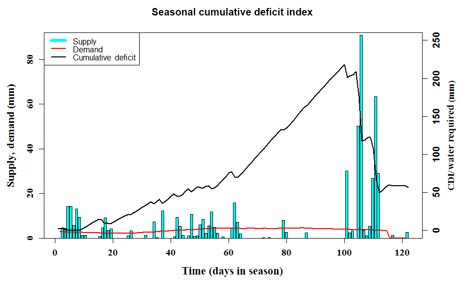
Figure 1A plot of the cumulative deficit index (CDI) for the JJAS season in a randomly selected year in our data set. The plot depicts the change in CDI as rainfall distribution, and crop water requirement varies over the given monsoon season. The vertical cyan bars are the daily rainfall magnitudes, the slowly changing red line is the crop water requirement (demand) and the black time series is the CDI itself. Notice how CDI increases as rainfall is either low in magnitude or sparsely distributed in certain periods of time in the season.
The water use for a given crop is estimated based on the expected growth stage and daily evapotranspiration as
In Eq. (2), is the crop coefficient, which is the ratio of actual evapotranspiration (ETa) of a given crop under non-stressed conditions to the reference crop evaporation (ET0). It represents crop-specific water use at various growth stages of the crop and is typically derived empirically based on local climatic conditions (Doorenbose and Pruitt, 1977). The accumulated deficit over a season is then given as
In Eq. (3), deficitj,d refers to the accumulated daily deficit for any given year with a crop growth period of ns days in the year, Dj,d to total daily water demand, Sj,d to the total daily effective rainfall for geographical location j and day d, t refers to a calendar or cropping year and n is the total number of years in the analysis. For an n-year record, seasonal water stress is evaluated as the maximum cumulative deficit in each season and is defined here as CDIj,t. CDI focuses on the rainfall distribution within the season relative to the crop water demand. It therefore accounts for the timing of planting, different stages of crop growth and the timing and distribution of rainfall in the season. The index may also be treated as a hydrologic index and forecasted exactly as one would forecast precipitation or temperature variables or any other water stress or drought index. Depending on the lead time of such forecasts, this can give farmers and other agricultural stakeholders a sufficient amount of planning and preparation time, thus providing them a critical edge in hedging agricultural water risk. This is critical for irrigation and water storage planning. The computation of CDI is illustrated in Fig. 1. This figure provides insights on the time-evolving vulnerability to stress arising from deficient rainfall and changes in crop demand.
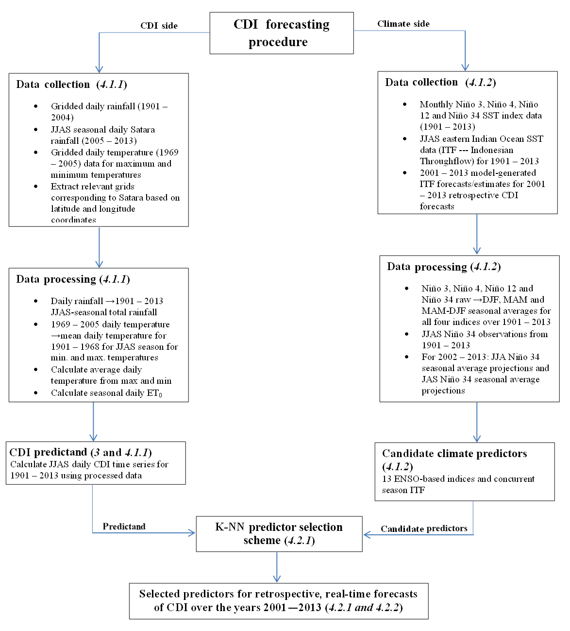
Figure 2Flowchart depicting the entire forecasting procedure for potato-based CDI in Satara, Maharashtra, India. The steps are categorized as data collection, data processing, predictand/predictor calculation, all of which converge to predictor selection and forecast modeling. The section number of the paper in which these steps are covered is written in italics next to the category. A brief summary of each step is given, one for the steps used in CDI calculation and another for the steps used in processing the candidate predictors from climate.
We provide an application of our general approach to forecast CDI for potatoes grown in the Satara district in Maharashtra, India as an application. The Satara district in Maharashtra is one of the primary regions for sourcing potatoes during the monsoon season (June–September). Satara supplies the majority of the potatoes processed by the Frito–Lay manufacturing plant in Pune, Maharashtra (Economic Times, 2013). The potato is a major cash crop in Maharashtra and accounts for at least 75 % of total production (Nikam et al., 2008). The average annual rainfall in this arid to semi-arid region is around 350 mm with high inter-annual variability. The region has experienced four droughts (seasonal rainfall below long-term average) since 2001. The ability to predict such droughts with a reasonable accuracy at lead times of 3 to 6 months could suggest ways of adapting existing agricultural operations to the anticipated conditions and minimizing the impacts of droughts on the agricultural supply chain. Hence, we develop, present and evaluate the results from retrospective forecasts of CDI for the monsoon season over the period 2001–2013. The June–July–August–September (JJAS) season is the growing season for potatoes in the Satara district. It is also the core monsoon season for the Indian sub-continent. The forecasts use climate data from 3 to 6 months prior to the beginning of the monsoon season as predictors, and forecasts are to be issued in May, 1 month prior to monsoon onset. This section discusses the full forecasting procedure used to predict CDI for potatoes grown during the JJAS monsoon season in Satara, India. This discussion covers all data used, the data processing steps, the prediction selection routine and its results and the forecasting model itself. Figure 2 presents a flowchart summarizing the entire process.
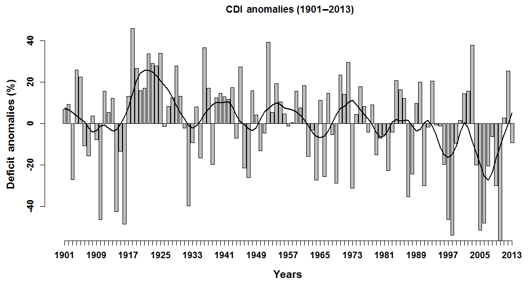
Figure 3Bar plot showing the CDI percent deficit anomalies for each of the years/growing seasons under consideration (1901–2013). The black, smooth time series is produced by an 11-year LOWESS smoothing of the CDI percent deficit anomalies and is meant to show the critical trends in the CDI over the entire 1901–2013 period.
4.1 Data collection and processing
4.1.1 Precipitation and temperature data and the CDI
Gridded daily rainfall data from 1901–2004 available at 1∘ × 1∘ spatial resolution from the India Meteorological Department (Rajeevan et al., 2006) and gridded daily temperature data from 1969–2005 available at the same spatial resolution from India Meteorological Department are used in this study. Since the daily temperature data are available only for 37 years, we used the daily climatology, i.e., the mean daily temperature, for the remaining 77 years (Devineni et al., 2013). The daily climate time series grids were spatially averaged over the Satara district. This process resulted in a time series of daily precipitation and temperature estimates for 104 years. The daily reference crop evapotranspiration (ET0) was developed based on the daily time series of minimum, mean and maximum temperature data and extraterrestrial solar radiation (Hargreaves and Samani, 1982). The Hargreaves method is used globally to predict ET0 in regions where data availability is limited to air temperature data (Allen et al., 1998). Seasonal daily rainfall data from 2005 to 2013 for the Satara district were collected separately from a website maintained by the Agricultural Department of Maharashtra State and used to augment the 104 years of rainfall and temperature data. The CDI was computed for each of these 113 seasons using the daily rainfall data and reference crop evapotranspiration. This will serve as the predictand for our forecast model. We remind the reader that Fig. 1 illustrates the computation of CDI.
CDI as a water stress measure is a proxy of not only crop water stress but also irrigation and water storage requirements. Consider Fig. 1. When daily seasonal rainfall is low or when rainfall enters an inactive phase for a considerable period of time, as displayed by the vertical cyan bars, the amount of daily accumulated water deficit increases to reflect the disparity between water supplied as rainfall and the water required by the crop to sustain itself, as displayed by the red curve in Fig. 1. The highest point, or peak, on the black deficit time series in Fig. 1 is the value of CDI, and it prepares us for the worst-case scenario of a deficient water supply for the crop. This can be calculated for multiple crops, with each CDI value depending on the specific crop's water demand and the location and time of planting. This gives the stakeholder a conservative estimate of how much additional water is needed beyond what nature is willing to supply in order to maintain critical yields while apportioning water resources intelligently. Since agriculture tends to be one of the largest consumers of water – about 70 % of all the world's freshwater withdrawals go towards irrigation use (USGS, 2017) in addition to what is rainfed – this is an integral part of water resource management.
The annual time series of the CDI computed for the JJAS season (referred to as the Kharif season on the Indian subcontinent) in Satara is presented in Fig. 3. We have standardized the CDI values as the percentage difference each year from the 113-year average of CDI. The long-term average CDI for growing potatoes in Satara is 241 mm. This is equivalent to approximately 975.3 m3 of water used for irrigating a 4046.86 m2 farm of potatoes on average throughout the season. The percent differences in Fig. 3 refer to percentages of this number, i.e., a 10 % increase in CDI indicates an additional requirement of 97.5 m3. From Fig. 3, it is clear that (a) Satara experiences recurrent droughts with intermediate wet periods and (b) there is year-to-year persistence in the incidence of these droughts. Such variations and epochal changes are typically modulated through large-scale global climate patterns. Investigating the relationship between the monsoon deficit and the large-scale climate teleconnections could enable the development of models that can be used to understand and predict the variability in the CDI in the region.
4.1.2 Climate precursors and climate data
Our goal was to develop a simple statistical model for predicting the CDI for potatoes grown in Satara. The generalized climate forecast models available at low spatial resolution are not specific enough for this task. Consequently, the first objective was to identify appropriate climate predictors before the monsoon starts in June. There is an extensive history of developing long-range predictions of monsoon rainfall that are based on various regional to large-scale climate predictors (Walker, 1924; Thapliyal, 1987). A variety of seasonal forecasts of the Indian summer monsoon rainfall (ISMR) are documented and available for reference (Gadgil et al., 2007; Kumar et al., 1995).
It is well established that inter-annual climate modes such as ENSO associated with anomalous sea surface temperature (SST) conditions in the tropical Pacific Ocean influence the inter-annual variability of ISMR (Parthasarathy and Pant, 1985; Shukla and Paolino, 1983). Anomalously warm tropical eastern Pacific SSTs (El Niño) are associated with a drier-than-normal ISMR, whereas anomalously cool tropical eastern Pacific SSTs (La Niña) are associated with a wetter-than-normal ISMR (Sikka, 1980; Parthasarathy and Pant, 1985; Rasmusson and Carpenter, 1983). Ihara et al. (2007) have suggested that the ENSO warm (cool) phases shift the location of the tropical Walker circulation and cause deficient (excessive) rainfall by suppressing (enhancing) the convection over India. Hence, ENSO indices were chosen to be among the candidate predictors for the forecast model. Raw monthly SST data for the Niño 3, Niño 4, Niño 12 and Niño 34 indices were taken from the Royal Netherlands Meteorological Institute (KNMI) climate explorer database (KNMI, 2014).
For each given raw ENSO index (3, 4, 12 and 34), we considered three different types of derived ENSO indices: a December–January–February (DJF) seasonal average, a March–April–May (MAM) seasonal average, and a MAM minus DJF (MAM − DJF) differenced time series. Among the Niño indices calculated, the change in the tropical Pacific SSTs from December to May (MAM − DJF trend) was found to be of significance by previous investigators. Shukla and Paolino (1983) found the correlation coefficient between the MAM–DJF trend pressure anomalies and the ISMR to be a significant −0.42. Their investigation showed that the Darwin pressure anomalies decrease from DJF to MAM before the occurrence of heavy monsoon rainfall and increase prior to the occurrence of deficit monsoon rainfall. Parthasarathy et al. (1988) found the correlation coefficient between this winter-to-spring trend and ISMR over the period 1951–1980 to be between 0.40 and 0.52 in magnitude, depending on the specific region within the tropical pacific. Hence, MAM-DJF trends from Niño 3, Niño 4, Niño 12 and Niño 34 were considered to be potential model predictors. Parthasarathy et al. (1988) found that the MAM-averaged tropical Pacific SSTs over the box 14 to 20∘ N, 176∘ E to 160∘ W had a correlation of −0.40 with ISMR, convincing us to consider this average as well. In addition to the MAM and MAM − DJF averages, we computed the winter season (DJF) average, although DJF-averaged tropical Pacific SSTs were not found to be significant in the literature. However, it is worth noting that Parthasarathy et al. (1988) found that the correlation coefficient between the Darwin SLP during the DJF season and ISMR was +0.39. As the concurrent season (JJAS) state of ENSO has an important, well-documented impact on ISMR, we also elected to include the Niño 34 JJAS average. As mentioned earlier, an El Niño event during the JJAS season is strongly associated with an anomalously dry JJAS rainfall season in India, while a La Niña event during the JJAS season is strongly associated with an anomalously wet JJAS rainfall season in India, prompting our choice. We coupled the JJAS seasonal average for the Niño 34 index with forecasts of the JJA and JAS seasonal averages for the Niño 34 index. These forecasts were obtained from the International Research Institute for Climate and Society (IRI) ENSO forecast page and covered the period 2002–2013. These forecasts can be used to forecast JJAS monsoon CDI in place of the observed Niño 34 JJAS values on a real-time basis. These forecasted values were averages of the projections from at least six distinct statistical/dynamical models, with one average for the JJA season and one average for the JAS season. Together, we start with a total of 13 ENSO-based indices.

Figure 4Spearman's rank correlation between the CDI in Satara and SST field during the same JJAS season. SST region in the Indian Ocean (red box) that influences the CDI has a statistically significant correlation at the 95 % significance level.
Other candidate predictor variables include concurrent season (JJAS) eastern Indian Ocean SSTs known as the Indonesian Throughflow or ITF. Warm, low-salinity water from the Pacific is introduced into the Indian Ocean via the ITF and is considered to be an integral component in the heat and hydrological budget of the Indian Ocean (Gordon et al., 1997). The ITF waters are also believed to influence SSTs and associated ocean–atmosphere coupling within the Indian Ocean, making it an important aspect of monsoon climate research (Gordon et al., 1997). Thus, the ITF was also selected to be a candidate predictor in the model. During the JJAS monsoon season, the ITF is strengthened considerably, allowing an abundant amount of relatively warm water to be injected into the Indian Ocean. Eastern Indian Ocean SSTs during the JJAS season correspond to enhanced (suppressed) atmospheric convection during the anomalous warming (cooling) of the Indian Ocean waters, which in turn supplies (robs) the developing monsoon of much-needed moisture. We found that the Spearman's rank correlation coefficient between CDI in Satara and the average SST anomalies over 20∘ N and 5∘ S and 100 and 130∘ E (the region representing ITF) during the JJAS season is around −0.35 (statistically significant at the 95 % level), suggesting that warm conditions in the ITF region result in below-normal CDI, or low crop water stress. Figure 4 presents the field correlation map of SST anomalies with CDI. For these reasons, we chose the concurrent season ITF data to be a candidate predictor. The ITF data were collected from the IRI data library and consist of two components, namely an observed component and a forecasted component. The observations consist of measured eastern Indian Ocean SST anomalies during the JJAS season from 1901 to 2013. The forecasts consist of JJAS-season ITF values retrospective of the ECHAM4.5 global climate model and cover the period 2001–2013. Skillful forecasts for the tropical SSTs based on coupled ocean–atmosphere general circulation models have been in operation from various climate centers since 1998. Hence, in the forecasting scheme, we used the ITF derived from the forecasted SST state issued in May from the ECHAM4.5 operational forecasting center (available from IRI data library: http://iridl.ldeo.columbia.edu/SOURCES/.IRI/.FD/.ECHAM4p5/.Forecast/.ca_sst/.ensemble24/ (last access: 5 February 2017); Li and Goddard, 2005; van den Dool, 2007; Roeckner et al., 1996). The observed JJAS ITF data are used to train the model, while the retrospective JJAS ITF forecasts are used to make forecasts for the years 2001–2013.
4.2 The forecasting procedure
4.2.1 Predictor selection
Given a pool of candidate predictors, the next step is to select the best subset of those predictors. The predictors used in the forecasting model were chosen based on an exhaustive search method. In the exhaustive search method, all possible combinations of the candidate predictor variables are used to develop models that are cross-validated on historical data. Skill metrics are then used to compare the predictive accuracy of each combination. In the present study, we began with 113 years of CDI data and fourteen candidates: Niño 3 DJF, Niño 3 MAM, Niño 3 MAM − DJF, Niño 4 DJF, Niño 4 MAM, Niño 4 MAM − DJF, Niño 12 DJF, Niño 12 MAM, Niño 12 MAM − DJF, Niño 34 DJF, Niño 34 MAM, Niño 34 MAM − DJF, Niño 34 JJAS and ITF. The exhaustive search method utilized the k-NN cross-validation algorithm and 40 years of training data (1901–1940) to build forecast distributions for each of the years 1941–2013. At each step, the training data were updated to include data from all of the years up to the year being cross-validated. Thus, we always only use the historical data and update the model each year with the information from the previous year, much as a regular user of the forecast system would have to do. These forecasting distributions, built over a 73-year record (1941 to 2013) were created successively for every unique combination of two variables, every unique combination of three variables, and so on until we reached the entire pool of predictors.
For each and every possible unique combination of the predictor variables, we obtain a matrix of 73 columns. For each of these 73 years, the squared error and ranked probability score (Epstein, 1969; Murphy, 1969, 1971; Candille and Talagrand, 2005) were computed, and from this the root-mean-squared error (RMSE) and ranked probability skill score (RPSS) were computed. In this manner, a single RPSS value and RMSE value were calculated for every possible combination of the predictor variables. We chose the following combination of predictors based on the relative optimality of both their RPSS and RMSE scores: Niño 12 MAM − DJF, Niño 34 MAM − DJF and ITF, and this set of variables had an RMSE of 49.25 mm of required (JJAS) seasonal water storage and an RPSS of 0.26. We devised a simple but effective decision rule for determining the optimal choice of predictors based on ranking the metric values. This is especially useful when the number of combinations of variables is unwieldy. Optimality was determined by assigning a rank number to the RMSE and RPSS values in such a way that the first number was assigned to the lowest RMSE value, the second to the second lowest RMSE value, and so on, and the first number was assigned to the largest RPSS value, the second to the second largest RPSS value, and so on. For a fixed number of cross-validated predictor candidates for each RMSE/RPSS pair and for one pair of each combination of predictors, we determined an RMSE and RPSS rank and took the sum of these ranks. The smallest of these sums corresponds to the best or optimal set of predictors among all possible sets of cross-validated predictors. We then compared the ranked sum while considering the number of predictors in order to choose the best set of predictors. The chosen trio of predictors mentioned above had the unequivocally highest value of RPSS and second lowest RMSE value out of all possible combinations of the original set of 17 candidates, the lowest RMSE being only slightly smaller at 48.92 mm. Conceptually, this procedure is similar to the “best subsets regression” or “step-wise regression” (Helsel and Hirsch, 2002), but in the spirit of using the k-NN algorithm for forecasting, we designed this selection scheme to use the k-NN algorithm instead.
CDI forecasts were subsequently made using the selected set of predictors. The forecast procedure is tested using the leave-one-out cross-validation method. Each historical observation is omitted in turn, and the model is developed using the remaining years of data. A prediction of the observation that was not kept in the model-building set is then made and compared with the actual outcome for that year. Results from a variant of this approach are presented in the next section. The CDI for the 2001 Kharif season is predicted using the model developed based on data from 1901 to 2000. Similarly, the CDI for 2002 is predicted based on the model that is developed using the data from 1901–2001. Thus, as we move from year to year, we update the model observations and predict the future state.
4.2.2 The k-nearest neighbors real-time forecasting model
The forecasts were developed using a non-parametric k-nearest neighbors (k-NN) model. This is a data-driven approach that develops a conditional probability distribution of the CDI given the predictors by first identifying the k-historical climate conditions that are most similar to the current values of the climate predictors and then randomly drawing the vector of CDI values in the historical data that correspond to these k neighbors. The neighbors are weighted so that the closer or more similar neighbors are chosen more often than those further away. The key steps are as follows.
Let X be the design matrix of size n×p, where p = number of predictors selected from the original pool of candidates. Let xi denote the ith row of X. Hence, xi is a vector containing the values of each of the p predictor variables during year i. In denoting the current values of the predictors by xc, the idea is to find k such predictor vectors from the historical record (i.e., find k values of xi with i<c) that are most “similar” to the value of xc and use this information to construct a sampling distribution of CDI from which we can issue probabilistic forecasts. The number of neighbors in the model, or k, represents the number of degrees of freedom in the model, and should be chosen with care, as the choice of k affects the skewness and level of uncertainty in the sampling distributions. After trying several different values for k, we found an optimal value to be k=25. Rajagopalan and Lall (1999) recommend that, as a rule of thumb based on asymptotic arguments, k be roughly equal to , where n = the total number of observations. In our situation, it was evident that we required more neighbors than this rule would allow due to the skewness and variance apparent in the sampling distributions when using only 11 or fewer neighbors. Lall and Sharma (1996) note that if their discrete kernel is used for resampling the conditional bootstrap, then the weights for further neighbors will decrease. Hence, choosing a larger k may reduce the variance in the estimate while potentially increasing the bias in the estimate of the conditional distribution. Cross-validation can also be used to choose an optimal value for k in a given setting.
Let y be the n-dimensional vector of seasonal CDI values, each component of which represents the aggregate water deficit level over the JJAS growing season of every year in the historical record. Assume that y has been centered and normalized by its historical average to produce mean-normalized anomalies. The first step was to consider the individual distance values (with a specified metric) between xc and xi for i = 1, …, c−1. The chosen distance metric for our k-NN model was the Mahalanobis distance (Mahalanobis, 1936), represented as
where Σ is the covariance matrix of the training values in X. The Mahalanobis distance measure judges point separations in a metric space based on statistical dissimilarity, as opposed to a solely physical distance. Hence, the level of similarity between predictor values across different years is determined by the orientation and location of each point relative to the scatterplot of the predictor data. Large distances from xc represent predictor values that are statistically anomalous in the context of the predictor data. After the Mahalanobis distances had been calculated, the k-smallest distance values, with k=25, were selected and the corresponding years in which these distances occurred were noted. These years, hereby referred to as the analog years, are the years during which the predictor signals were the most similar to those of the current year. The vector-valued predictors during these analog years are referred to as the neighbors of xc.
The final step was to resample CDI values from the analog years. The resampling technique employed is a nonparametric method known as the bootstrap (Efron, 1979; Efron and Tibshirani, 1993). The idea behind the bootstrap component is to sample with replacement from a pool of data using the underlying distribution that generated the data to guide the sampling process. We chose not to assign a parametric family of distributions to the CDI data and instead estimated its underlying distribution non-parametrically using a kernel density estimator. This non-parametric method of k-NN bootstrapping was first introduced in Lall and Sharma (1996). Applications of the methods using different variants have since been presented (for example, see Rajagopalan and Lall, 1999; Souza and Lall, 2003 and references therein). We employed the same discrete resampling kernel proposed in Lall and Sharma (1996), which has the general form with , where j is the rank of each neighbor of xc, a rank of j=1 is assigned to the closest neighbor and a rank of j=k is assigned to the most distant neighbor. Our strategy was to build this kernel density estimator based on the ranks of the selected neighbors and resample the predictands from these analog years. We resampled from the 25 analog CDI values 1000 times, and each of the 25 values was resampled proportionally to the probability of its occurrence as determined by the density estimator.
4.2.3 Analyzing the k-NN results
The way in which model results are interpreted and presented is important for potential stakeholders. In this case study, our interest was in forecasting the CDI for a given potato growing season in Satara. The information from these forecasts can be of great use to potato farmers in Satara as well as corporations with investments in these farming areas. This necessitates a clear and concise communication of the forecast results.
The output of the k-NN model was a time series for each forecasted year consisting of 1000 realizations. This is the sampling distribution for the CDI and consists of mean-normalized anomaly values from the analog years converted to percentage values. As stated in the previous section, the deficit value from each analog year in the sampling distribution is represented proportionally to its probability of occurrence as assigned by a kernel density estimator. The sampling distribution is used to issue one-season-ahead probabilistic forecasts (i.e., the likelihood of a deficit for the forthcoming growing season). There are a whole slew of possibilities when it comes to using these sampling distributions for probability-based forecasts. Our approach consists of the following steps for a given forecasted growing season:
-
A box plot depicting the sampling distribution with the observed percent anomaly value superimposed on the box plot for every growing season forecasted. In using predictand anomalies, the historical mean becomes the zero line in the coordinate plane of the box plot.
-
A three-category forecasting system with the categories “above normal”, “normal” and “below normal” is used, provided that the historical mean and climatology are the threshold that is desired.
-
The probabilities for the categories specified in step 2 from the sampling distribution generated in step 1 are calculated and used to evaluate the accuracy and strength of the forecast based on contingency metrics such as hit rates and false alarms.
-
To get a sense of the spread and variability in the box plot distribution, the Interquartile Range (IQR) is calculated.
-
The value of the observed percent anomaly of the predictand is compared with the category in which the majority of the probability mass of the sampling distribution lies. This is of central importance in getting a basic sense of the accuracy of the forecast.
In general, the construction of such a sampling distribution allows the investigator the freedom to calculate probabilities on many different thresholds. The thresholds should be defined by the particular application and the needs of any stakeholders involved.
5.1 CDI forecast results and comparison with IMD monsoon forecasts
We hereby present the results of the CDI forecasts for the 2001–2013 JJAS seasons in the Satara district, Maharashtra, India. Forecasts are specifically made in the interest of irrigation requirements for potatoes grown in the Satara district, and we discuss the results in this context. The output of the k-NN model is the forecasting distributions for CDI of the 13 years and a series of box plots representing these forecast distributions as shown in Fig. 5. The probabilities calculated from these distributions are shown in Table 1, columns 2 and 3.
Figure 5 shows a series of box plot diagrams depicting the k-NN forecast distributions for CDI in the years 2001–2013. All calculations in this figure, including the construction of the distributions themselves, were done using anomalies of the predictand rather than the raw predictands. The anomalies were calculated by subtracting the 1901–2013 mean from the data, dividing by this mean value and converting the quotient to a percentage. The idea is to gauge the level of the seasonal crop water deficit in a forecasted year with respect to the level of crop water deficit that has occurred on average over the entire historical record. This should address the question of how “normal” or “abnormal” a given level of deficit over the course of a season is with respect to everything we have seen or experienced thus far. Given that the forecast is developed one season ahead, the sign of a strong shift in the probability will alert the decision makers to an anticipated deficit or surplus event.

Figure 5Box plot diagrams depicting the k-NN forecast distributions for CDI in the years 2001–2013 for potatoes grown in the Satara district, Maharashtra, India. Longer, more stretched out boxes indicate a greater degree of variability, or uncertainty, in the forecast distribution. Boxes in which the median is grossly off-center indicates that the forecast distribution is heavily skewed. Anomalies with respect to the climatology of the predictand were used in the box plot calculations. As the results are presented in terms of the percent anomalies, the historical average is located at zero. The triangles represent the observations as percent anomalies about the mean. Boxes that have been shaded in gray indicate years during which identical directionality was observed, whereas boxes that are white indicate years during which dissimilar directionality was observed.
We have created two general possibilities; the observed percent anomaly values (triangles in Fig. 5) can be positive or negative. As the forecasts were carried out using anomalies instead of raw values, the 1901–2013 historical average is repositioned as the zero line in Fig. 5. We calculate the probability under the k-NN forecast distribution of observing positive (negative) deficit anomalies for each year in 2001–2013. These are retrospective forecasts in the sense that these anomalies were already observed and recorded but were not used in building the model. These probabilities, corresponding observed percent anomalies and IQR values are presented in Table 1. The utility of these forecasts are discussed in Sect. 5.2.
Given the above information, we judge the accuracy of the forecasts during any given year on a few simple criteria, namely the directional agreement between the observed percent predictand anomaly and the median of the forecast distribution (Fig. 5), the joint consideration of the forecast probabilities and the observed percent anomaly (Table 1, columns 2–4) and the level of uncertainty in the forecast distribution (Fig. 5 and Table 1, column 5). Uncertainty is measured by the IQR of the box plot distribution. In the present context, we say that a forecast for a given year has identical directionality (with respect to the observation) if both the median of this forecast and the observation (as a percent anomaly) are either positive (above the historical average) or negative (at or below the historical average). The absence of identical directionality will be called dissimilar directionality.
The box-and-whisker plots shown in Fig. 5 for each year illustrate the range of possible values of the CDI for that year. We have identical directionalities for the years 2001, 2004, 2005, 2006, 2007, 2010, 2011, 2012 and 2013. For the years 2001, 2011 and 2012, the model correctly forecasted that the water stress conditions for the Maharastran potatoes would be above the CDI climatology. We can see from Fig. 5 that both the observed percent anomalies (triangles) and the medians for all of these forecasted years are positive. Additionally, Table 1, column 2 shows that the majority of the probability mass of the k-NN distribution is placed in the “Above Mean” category for 2001, 2011 and 2012, while column 4 shows that for these years, the observed CDI anomalies are positive. Similarly, for the years 2004, 2005, 2006, 2007, 2010 and 2013, the model correctly forecasted that water stress conditions for the potatoes would be below the historical average, and this can be seen from Fig. 5, where the observed anomalies and the medians for all of these forecasted years are negative. Similarly, Table 1, column 3 shows that the majority of the probability mass from the k-NN forecasting model was placed on the “Below Mean” category for these years, and the corresponding observed CDI anomalies are also negative. For the years 2002, 2003, 2008 and 2009, we have dissimilar directionalities. The forecasts suggest higher probability values for below average CDIs during 2002 and 2003, whereas positive anomalies were observed for these years. Similarly, the forecasts for 2008 and 2009 placed the majority of the probability mass on CDIs that are higher than average, suggesting that these years were likely to see higher than normal potato water stress. However, the observed CDI anomalies were negative, implying the opposite scenario.
Table 1The table below shows important statistics calculated from k-NN forecasts of CDI. In particular, column 2 displays the probabilities of the CDI for a particular season being above the CDI climatology. These probabilities are calculated from the k-NN sampling distribution, which in turn is simulated from historical values of the CDI based on the nearest neighbors determined in the predictor variable space. Column 3 shows the complementary probabilities of values being below this historical average. The forecasts for years 2001–2013 are retrospective and may serve as cross-validation for the k-NN model. Column 4 shows the values of the actual (observed) CDI anomalies with respect to the 1901–2013 climatology as percentages. A negative value implies that the actual CDI value was below the historical average by the given percentage. The rounded IQR values are shown in the final column of the table.
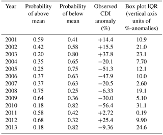
Table 2The results of the k-NN generated CDI forecasts, including the most likely category (AM = Above Mean, BM = Below Mean) along with the corresponding k-NN assigned probability value expressed as a percentage in parentheses next to it (column 2), the category in which the observed anomaly value resides (column 3) and the hit/miss/false alarm designations corresponding to these results (column 4).
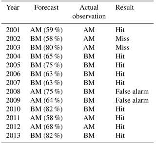
Table 3A comparison of the CDI forecasts and the JJAS total seasonal precipitation forecasts generated by the India Meteorological Department (IMD). Column 2 is a repeat of column 4 in Table 2; a record of the accuracy of CDI forecasts is expressed in terms of hits and misses. Column 3 contains the forecasts issued by IMD, and column 4 is the actual observations of JJAS seasonal total rainfall using rainfall data from the Satara district itself. The fifth and final column of Table 3 shows the accuracy of the IMD forecasts in terms of hits and misses using their own 5-category system.
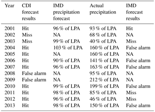
NA: not available.
We say that a hit has occurred if identical directionality is observed. A miss occurs if the forecast implies below average water stress, but the observation shows above average water stress. Finally, a false alarm occurs if the forecast implies above average water stress, while the observation shows below average water stress. Table 2 shows that the hit rate of the k-NN forecasts is 9∕13, the miss rate is 2∕13 and the false alarm rate is 2∕13. Table 3 shows a comparison of our CDI forecasts with seasonal total precipitation forecasts of the India Meteorological Department, abbreviated as IMD. The IMD forecast presented here for 2001 is long-range for precipitation in the JJAS season over three climatically homogeneous regions in India, namely northwestern India, peninsular India, and northeastern India. Since Maharashtra is in peninsular India, we refer to this forecast. For 2001, the forecast result was categorized as either normal, above normal or below normal. “Normal” is defined as being within ±10 % of the long-period average, or LPA. Beginning in 2003, the IMD began offering two-stage forecasts, the first released in mid-April using data up to March and an update in June using data up to May. For both 2011 and 2013, we used the initial countrywide forecast, as the updated forecasts for JJAS could not be found. In 2003, IMD began to divide their forecast results into five categories, namely drought/deficient, below normal, near normal/normal, above normal and excess. “Deficient” (drought) is defined as JJAS total seasonal rainfall that is less than 90 % of the long period average (LPA). “Below normal” is defined as the JJAS rainfall that is 90 %–96 % of the LPA, “normal” (sometimes called “near normal”) is defined as the JJAS rainfall that is 96 %–104 % of the LPA, “above normal” is defined as the JJAS rainfall that is 104 %–110 % of the LPA and “excess” is defined as the JJAS rainfall that is more than 110 % of the LPA. The IMD forecasts are reported as percentages of the LPA, as shown in column 3 of Table 3. Based off of the categories defined by IMD and comparing these forecasts with actual JJAS seasonal total precipitation anomalies from our gridded rainfall data set, where these anomalies have been calculated with respect to the long period average defined as 1901–2013, we classify each forecast as a hit, miss or false alarm, as was done with the CDI forecasts. The hit rate for IMD is 1∕9, the miss rate is 3∕9 and the false alarm rate is 5∕9. We must bear in mind that the total precipitation forecasts given here are for an entire region that includes the state of Maharashtra, whereas our CDI forecasts are generated based on CDI calculations from the target location of Satara, Maharashtra, India. Hence, our CDI anomalies reflect the conditions of Satara on a much higher resolution than the coarse IMD precipitation anomalies. Furthermore, we are comparing IMD forecasts with actual precipitation totals from Satara, computed with respect to the 1901–2013 LPA instead of the 1951–2000 LPA of IMD under the reasonable assumption that the LPA does not change much between those two definitions. While the IMD monsoon forecasts can provide a broad regional understanding of the monsoon conditions, supplementing them with targeted crop-specific forecasts such as ours will help improve agricultural planning and regional water management. To conclude, we used observations for ITF and Nino 34 JJAS to generate CDI forecasts for the years 1976–2000 and augmented these forecasts with the 2001–2013 CDI forecasts depicted in Fig. 5. Running the forecasts for a longer period of time, which in this case is 38 years, ensures the robustness of the procedure. The hit, false alarm and miss rates resulting from this extended retrospective, adaptive forecast are 24∕38 hits, 9∕38 false alarms and 5∕38 misses. Hence, we are observing 63 % hits, which indicates a fairly good, robust forecasting procedure for an informative crop water stress index.
We define a strong forecast as a forecast in which the probability assigned to one of the two categories is at least 60 %. In our situation, 10 out of the 13 years witnessed strong forecasts. A weak forecast runs the risk of being less informative to decision makers, whereas a strong forecast is much more assertive and definitive; hence, decisions can be made more easily with a strong forecast. The forecasts were also correct for 7 of these 10 years, as seen in Table 2. The forecasts were correct but slightly weak for 2 years (2001 and 2011). If one considers acting only if the probability associated with a CDI forecast is at least 60 %, then the forecast is correct 7 out of 10 times. Raising this to 66 % leads to the correct classification of 4 out of 6 years.
It is important to point out that one should also consider the uncertainty (column five in Table 1) when evaluating the power of the forecasts. Knowing the uncertainty is useful, since years in which the uncertainty in the forecast is low and there is a strong indication for the CDI may lead to different risk management actions than years in which the forecast has strong directional change but is also marked by high uncertainty.
5.2 Discussion of results: the utility of targeted forecasts
It is natural to ask how one might go about using CDI forecasts. Here is a short example of how these forecasts can facilitate decision-making. In 2001, irrigating or ensuring water storage equal to 0.2757 m3 per m2 for the potatoes would have been the ideal situation, as this is equal to 14.4 % above the average CDI value of 241 mm of the water storage equivalent. However, this exact amount cannot be known in the absence of the observed CDI anomaly, which is found in column four of Table 1. Using the median as a plausible estimate for the true anomaly value, roughly 0.2516 m3 per m2 would have been irrigated or stored instead. A more risk-averse decision maker may choose to use the upper quartile or even maximum of the k-NN generated sampling distribution as a proxy for the true anomaly value. Such decisions are often made on the basis of prior experience.
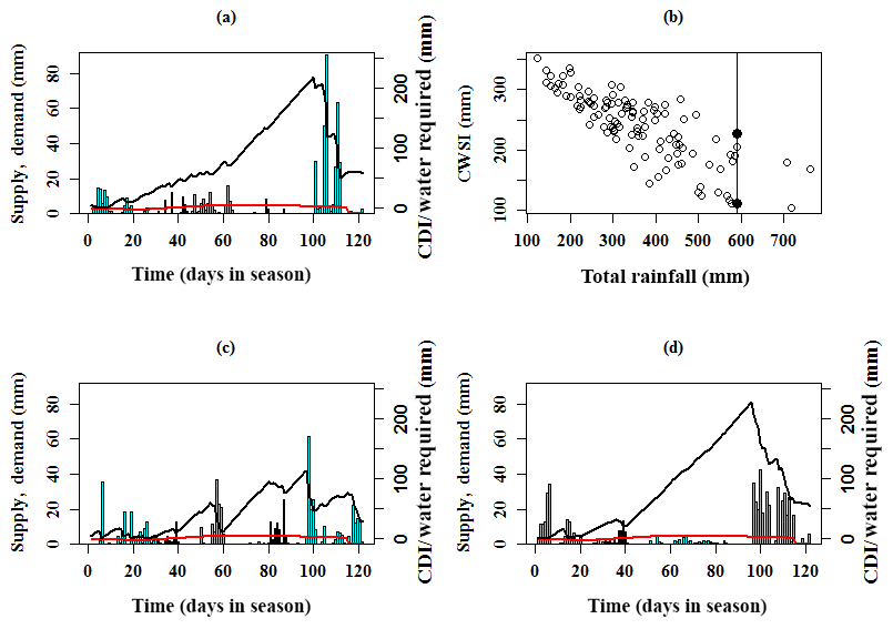
Figure 6The four panels pictured here depict the CDI in various ways. In (a, c, d), the blue bars represent daily seasonal rainfall levels (in mm), the red curve represents crop evaporative water demand (ET0) and the black time series is the CDI calculated based on this data. (a) illustrates the basic nature of CDI using the daily seasonal CDI time series from the JJAS growing season of 2013. Note that this time series is specifically calculated for potatoes grown in the Satara district of Maharashtra, India during the 2013 JJAS growing season. (b) shows a scatterplot of total rainfall across all growing seasons (1901–2013) and CDI across all growing seasons. A significant negative correlation between them is apparent from this scatterplot (Pearson correlation is −0.8, Spearman's rank correlation is −0.812, Kendall rank correlation is −0.623). This panel demonstrates two different growing seasons, with two different CDI values during which the total seasonal rainfall was the same. (c) is a seasonal CDI time series plot corresponding to the growing season, with the lower CDI value on the vertical line in (b). (d) is a seasonal CDI time series plot corresponding to the growing season, with the higher CDI value on the vertical line in (b).
Although total seasonal rainfall is sometimes used for agricultural water planning, CDI boasts a significant advantage over total seasonal rainfall in this capacity. CDI reliably accounts for water stress incurred by haphazard and erratic patterns of rainfall during the season. A total seasonal rainfall forecast that indicates a growing season with sufficient rainfall will not be reliable when rain throughout the season is erratically distributed in clusters of rainy days, whereby all of the rainfall in a given season occurs within a portion of the season, and the remainder of the season is virtually dry. This is a common occurrence in monsoonal climates and may have deleterious effects on crops that are vulnerable to prolonged dry periods and/or chunks of time during which rainfall is excessive. Long dry spells throughout the season that can be detrimental to drought-sensitive crops are not accounted for in a measure of total seasonal rainfall, making it possible for the seasonal rainfall to appear sufficient due to sporadic occurrences of large precipitation events. Consequently, it can also serve as a better indicator than regional rainfall to devise index-insurance products for agriculture, where crop specific indices can be developed (Skees, 2016). These characteristics of crop water stress must be accounted for in the proper planning and management of agricultural water resources.
To illustrate the aforementioned point further, we reference Fig. 6. In this figure, the varying rainfall distribution is indicated by the vertical bars, the crop demand is given by the horizontal line (primary y-axis) and the time series shows the cumulative deficit. Figure 6b shows 2 distinct years during which the total seasonal rainfall was 590 mm (vertical line). During one of these 2 years, the CDI value was 111 mm of water deficit for the potato crop, while the CDI value for the other year was 228 mm. This indicates that the water stress for a particular crop relies on both the magnitude and frequency of seasonal rainfall. When daily seasonal rainfall is more uniform, the daily deficit values do not have the chance to accumulate as much as when rainfall is less uniform and as a result, when there are persistent dry spells or long precipitation-inactive periods. Figure 6c shows the resulting cumulative deficit when daily rainfall occurs with greater frequency during the JJAS season and hence the total seasonal rainfall is distributed among the days of the growing season fairly uniformly. Figure 6d, located immediately to the right of Fig. 6c, shows the resulting cumulative deficit when rainfall is dominant during the first and last months of the JJAS season. While rainfall events do occur between those months, the magnitude of the rainfall is quite low, allowing the seasonal daily CDI time series to spike to a considerably higher maximum value (228 mm) than the CDI time series in Fig. 6c (111 mm maximum). The CDI time series recedes and recovers at the end of the season when the rainfall increases in magnitude. Hence, the CDI can discriminate between two monsoon seasons which have the same total rainfall but differ in that one may have rainfall distributed uniformly over the season through modest rainfall events, while the other may have a few intense rain events separated by long dry periods. As we can see, the latter gives rise to a much higher CDI.
An interesting and excellent discussion concerning the usability of such science is found in Dilling and Lemos (2011) and several papers cited therein. In the context of that discussion, we find that our forecasting procedure combines the “science push” and “demand pull” approaches to creating scientific usability. The impetus for crafting the CDI and, prior to that, independently developing the k-NN algorithm, was scientific. However, the decision to combine them and apply them to seasonal forecasting as we have done here was made with agricultural stakeholder interests in mind. As discussed in Dilling and Lemos (2011), the problem of overcoming informal institutional barriers to avail such seasonal forecasts, namely the idea that current methods of forecasting through weather and climate prediction centers are the only reliable methods, is one potentially faced by our methodology. If this is the case, this is unfortunate, as we feel that our targeted forecasting system is potentially very useful to stakeholders and decision-makers in relevant sectors.
A novel crop water stress index, the CDI, was developed here as a way of estimating water storage and irrigation requirements in the interest of agricultural water resources. As the management of water resources requires advanced knowledge of water risk, the main task accomplished here was the forecasting of the CDI as an effective method for understanding and hedging risk. This concept of forecasting the CDI for evaluating irrigation requirements was applied to a case study in the Satara district of Maharashtra, India, in which the CDI pertaining to potatoes grown in Satara during the southwest monsoon season was forecasted using large-scale climate indices as predictors in a semi-parametric k-nearest neighbors stochastic model that issues probabilistic forecasts. The climate indices used were defined either concurrent to the monsoon season or 3 to 6 months prior. Based on the hit and false alarm rates, the results achieved using our methodology were more favorable than precipitation forecasts conducted by the India Meteorological Department. We also observed in our method a greater tendency towards strong and informative forecasts.
This study developed a framework for quantifying and analyzing climate-induced agricultural risks. It is based on (a) developing a CDI for assessing crop-specific water risk, irrigation requirements and water storage needs for the agricultural sector, (b) investigating the sources of predictability for this indicator and (c) developing statistically verifiable models for issuing season-ahead probabilistic forecasts for evaluating water risk and irrigation needs. We can conclude that this is a useful approach in investigating irrigation requirements and that a bootstrap-based uncertainty estimation is useful for developing probability-based management models for optimizing agricultural decisions.
The CDI data used in this paper is available upon request of the contact author.
The authors declare that they have no conflict of interest.
This research was supported by the NSF grant 1360446 (Water Sustainability and Climate, Category 3) and the PSC-CUNY award 69729-00 47.
Partial support for the third and fourth authors is provided from PepsiCo
Inc. through the WATER RISKS AND SUSTAINABILITY grant. The statements
contained within the manuscript are not the opinions of the
funding agency or the US government but reflect the authors' opinions.
Edited by: Lixin Wang
Reviewed by: Vimal Mishra and two anonymous referees
Allen, R. G., Pereira, L. S., Raes, D., and Smith, M.: Crop Evapotranspiration – Guidelines for Computing Crop Water Requirements, FAO Irrigation and Drainage Paper 56, FAO of the UN, Rome, 15 pp., 1998.
Asoka, A. and Mishra, V.: Prediction of Vegetation Anomalies to Improve Food Security and Water Management in India, Geophys. Res. Lett., 42, 5290 –5298, 2015.
Belayneh, A. and Adamowski, J.: Standard Precipitation Index Drought Forecasting Using Neural Networks, Wavelet Neural Networks and Support Vector Regression, Applied Computational Intelligence and Soft Computing, Hindawi, London, UK, 13 pp., 2012.
Candille, G. and Talagrand, O.: Evaluation of Probabilistic Prediction Systems for a Scalar Variable, Q. J. Roy. Meteorol. Soc., 131, 2131 – 2150, 2005.
Chen, X., Naresh, D., Upmanu, L., Hao, Z., Dong, L., Ju, Q., Wang, J., and Wang, S.: China's water sustainability in the 21st century: a climate-informed water risk assessment covering multi-sector water demands, Hydrol. Earth Syst. Sci., 18, 1653–1662, https://doi.org/10.5194/hess-18-1653-2014, 2014.
Devineni, N., Perveen, S., and Lall, U.: Assessing Chronic and Climate Induced Water Risk Through Spatially Distributed Cumulative Deficit Measures: A New Picture of Water Sustainability in India, Water Resour. Res., 49, 2135–2145, 2013.
Devineni, N., Lall, U., Etienne, E., Shi, D., and Xi, C.: America's water risk: Current demand and climate variability, Geophys. Res. Lett., 42, 2285–2293, https://doi.org/10.1002/2015GL063487, 2015.
Dilling, L. and Lemos, M. C.: Creating usable science: Opportunities and constraints for climate knowledge use and their implications for science policy, Global Environ. Change, 21, 680–689, https://doi.org/10.1016/j.gloenvcha.2010.11.006, 2011.
Doorenbose, J. and Pruitt, W. O.: Guidelines for Predicting Crop Water Requirements, Irrigation and Drainage Paper 24, FAO of the UN, Rome, 154 pp., 1977.
Economic Times: India Times, available at: http://articles.economictimes.indiatimes.com/2013-09-25/news/42394669_1_drip-irrigation-farming-market (last access: 1 March 2018), 2013.
Efron, B.: Bootstrap Methods: Another Look at the Jacknife, Ann. Statist., 7, 1–26, 1979.
Efron, B. and Tibishirani, R.: An Introduction to the Bootstrap, Chapman and Hall, New York, 456 pp., 1993.
Epstein, E. S.: A Scoring System for Probability Forecasts of Ranked Categories, J. Appl. Meteorol., 8, 985–987, 1969.
Etienne, E., Devineni, N., Khanbilvardi, R., and Lall, U.: Development of a Demand Sensitive Drought Index and its Application for Agriculture over the Conterminous United States, J. Hydrol., 534, 219–229, https://doi.org/10.1016/j.jhydrol.2015.12.060, 2016.
Gadgil, S., Rajeevan, M., and Francis, P. A.: Monsoon Variability: Links to Major Oscillations Over the Equatorial Pacific and Indian Oceans, Curr. Sci. India, 93, 182–194, 2007.
Gordon, A. L., Ma, S., Olson, D. B., Hacker, P., Ffield, A., Talley, L. D., Wilson, D., and Baringer, M.: Advection and diffusion of Indonesian throughflow water within the Indian Ocean South Equatorial Current, Geoophys. Res. Lett., 24, 2573–2576, https://doi.org/10.1029/97GL01061, 1997.
Hargreaves, G. H. and Samani, Z. A.: Estimating Potential Evapotranspiration. J. Irrig. Drain. Div., 108, 225–230, 1982.
Heim Jr., R. R.: A Review of Twentieth-Century Drought Indices Used in the United States, B. Am. Meteorol. Soc., 83, 1149–1165, 2002.
Helsel, D. R. and Hirsch, R. M.: Statistical Methods in Water Resources, US Geological Survey, 467 pp., 2002.
Ho, M., Parthasarathy, V., Etienne, E., Russo, T., Devineni, N., and Lall, U.: America's water: Agricultural water demands and the response of groundwater, Geophys. Res. Lett., 43, 7546–7555, https://doi.org/10.1002/2016GL069797, 2016.
Ihara, C., Kushnir, Y., Cane, M. A., and de la Peña, V. H.: Indian summer monsoon rainfall and its link with ENSO and Indian Ocean climate indices, Int. J. Climatol., 27, 179–187, https://doi.org/10.1002/joc.1394, 2007.
Kar, S., Acharya, N., Mohanty, U. C., and Kulkarni, M. A.: Skill of Monthly Rainfall Forecasts Over India Using Multi-Model Ensemble Schemes, Int. J. Climatol., 32, 1271–1286, https://doi.org/10.1002/joc.2334, 2012.
KNMI Climate Explorer: available at: https://climexp.knmi.nl, last access: 1 January 2014.
Kumar, K. K., Sonam, M. K., and Kumar, R. K.: Seasonal Forecasting of Indian Summer Monsoon Rainfall: A Review, Weather, 50, 449–467, https://doi.org/10.1002/j.1477-8696.1995.tb06071.x, 1995.
Lall, U. and Sharma, A.: A Nearest Neighbor Bootstrap for Resampling Hydrologic Time Series, Water Resour. Res., 32, 679–693, https://doi.org/10.1029/95WR02966, 1996.
Li, S. and Goddard, L.: Retrospective Forecasts with the ECHAM4.5, AGCM IRI Tech. Report, 5–2 December 2005, International Research Institute for Climate and Society, Palisades, NY, 2005.
Liu, X. and Pan, Y.: Agricultural Drought Monitoring: Progress, Challenges, and Prospects, J. Geogr. Sci., 26, 750–767, https://doi.org/10.1007/s11442-016-1297-9, 2016.
Mahalanobis, P. C.: On the Generalized Distance in Statistics, P. Natl. Inst. Sci. India, 2, 49–55, 1936.
McKee, T. B., Doesken, N. J., and Kleist, J.: The Relationship of Drought Frequency and Duration to Time Scales, in: Eighth Conference on Applied Climatology, 17–22 January 1993, Anaheim, California, 1993.
Mishra, A. K. and Desai, V. R.: Drought Forecasting Using Stochastic Models, Stoch. Environ. Risk Res. A, 19, 326–339, https://doi.org/10.1007/s00477-005-0238-4, 2005.
Mishra, A. K. and Desai, V. R.: Drought Forecasting Using Feed-Forward Recursive Neural Network, Ecol. Model., 198, 127–138, https://doi.org/10.1016/j.ecolmodel.2006.04.017, 2006.
Mishra, A. K. and Singh, V. P.: A Review of Drought Concepts, J. Hydrol., 391, 202–216, 2010.
Murphy, A. H.: On the “ranked probability score”, J. Appl. Meteorol., 8, 988–989, 1969.
Murphy, A. H.: A Note on the Ranked Probability Score, J. Appl. Meteorol., 10, 155–156, 1971.
Nikam, A. V., Shendage, P. N., Jadhav, K. L., and Deokate, T. B.: Economics of Production of Kharif Potato in Satara, India, Int. J. Agricult. Sci., 4, 274–279, 2008.
Palmer, W. C.: Meteorological Drought, Research Paper No. 45, US Department of Commerce, Washington, D.C., 65 pp., 1965.
Parthasarathy, B. and Pant, G. B.: Seasonal Relationships Between Indian Summer Monsoon Rainfall and the Southern Oscillation, Int. J. Climatol., 5, 369–378, 1985.
Parthasarathy, B., Diaz, H. F., and Escheid, J. K.: Prediction of All-India Summer Monsoon Rainfall with Regional and Large-Scale Parameters, J. Geophys. Res., 93, 5341–5350, https://doi.org/10.1029/JD093iD05p05341, 1988.
Rajagopalan, B. and Lall, U.: A k-nearest neighbor simulator for daily precipitation and other weather variables, Water Resour. Res., 35, 3089–3101, 1999.
Rajeevan, M., Bhate, J., Kale, J. D., and Lal, B.: High Resolution Daily Gridded Rainfall Data for the Indian Region: Analysis of Break and Active Monsoon Spells, Curr. Sci. India, 91, 296–306, 2006.
Rasmusson, E. M. and Carpenter, T. H.: The Relationship Between Eastern Equatorial Pacific Sea Surface Temperature and Rainfall Over India and Sri Lanka, Mon. Weather Rev., 111, 517–528, 1983.
Rockstrom, J., Karlberg, L., Wani, S. P., Barron, J., Hatibu, N., Oweis, T., Bruggeman, A., Farahani, J., and Qiang, Z.: Managing Water in Rainfed Agriculture – The Need for a Paradigm Shift, Agr. Water Manage., 97, 543–550, https://doi.org/10.1016/j.agwat.2009.09.009, 2009.
Roeckner, E., Brokopf, R., Esch, M., Giorgetta, M., Hagemann, S., Kornblueh, L., Manzini, E., Schlese, U., and Schulzweida, U.: The atmospheric general circulation model ECHAM5: Model description and simulation of present-day climate, Rep. 218, Max-Planck-Institut für Meteorologie Hamburg, Germany, 90, 1996.
Serrano-Vicente, S. M., Beguería, S., and López-Moreno, J. I.: A Multiscalar Drought Index Sensitive to Global Warming: The Standardized Precipitation Evapotranspiration Index, J. Climate, 23, 1696–1718, https://doi.org/10.1175/2009JCLI2909.1, 2010.
Shah, R. D. and Mishra, V.: Utility of Global Ensemble Forecast System (GEFS) Reforecast for Medium-Range Drought Prediction in India, J. Hydrometeorol., 17, 1781–1800, https://doi.org/10.1175/JHM-D-15-0050.1, 2016.
Shah, R. D., Sahai, A. K., and Mishra, V.: Short to Sub-Seasonal Hydrologic Forecast to Manage Water and Agricultural Resources in India, Hydrol. Earth Syst. Sci., 21, 707–720, https://doi.org/10.5194/hess-21-707-2017, 2017.
Shukla, J. and Paolino, D. A.: The Southern Oscillation and Long-Range Forecasting of the Summer Monsoon Rainfall over India, Mon. Weather Rev., 111, 1830–1837, 1983.
Sikka, D. R.: Some aspects of the large-scale fluctuations of summer monsoon rainfall over India in relation to fluctuations in the planetary and regional scale circulation parameters, P. Indian As.-Earth, 89, 179–195, https://doi.org/10.1007/BF02913749, 1980.
Skees, J. R.: Innovations in Index Insurance for the Poor in Lower Income Countries, Agr. Resour. Econ. Rev., 37, 1–15, https://doi.org/10.1017/S1068280500002094, 2016.
Souza, F. A. and Lall, U.: Seasonal to Interannual Ensemble Streamflow Forecasts for Ceara, Brazil: Applications of Multivariate, Semiparametric Algorithm, Water Resour. Res., 39, 13, https://doi.org/10.1029/2002WR001373, 2003.
Thapliyal, V.: Prediction of Indian Monsoon Variability Evaluation and Prospects Including Development of a New Model, China Ocean Press, Beijing, 397–416, 1987.
USGS: Irrigation Water Use, available at: https://water.usgs.gov/edu/wuir.html (last access: 14 March 2018), 2017.
van den Dool, H. M.: Empirical Methods in Short-Term Climate Prediction, Oxford University Press, Oxford, 215 pp., 2007.
Walker, G. T.: Correlations in seasonal variations of weather, IX: A further study of world weather (World Weather II), Memoirs India Meteorol. Depart., 24, 275–332, 1924.
- Abstract
- Introduction
- A brief review of the current forecasting systems for water management in monsoonal climates
- The cumulative deficit index: background and scientific basis
- Case study: forecasting irrigation requirements for potatoes in Maharashtra, India
- Case study: forecast results and discussion
- Summary and conclusion
- Data availability
- Competing interests
- Acknowledgements
- References