the Creative Commons Attribution 4.0 License.
the Creative Commons Attribution 4.0 License.
 | 15 Oct 2018
Value of uncertain streamflow observations for hydrological modelling
Barbara Strobl
Jan Seibert
H. J. Ilja van Meerveld
Previous studies have shown that hydrological models can be parameterised using a limited number of streamflow measurements. Citizen science projects can collect such data for otherwise ungauged catchments but an important question is whether these observations are informative given that these streamflow estimates will be uncertain. We assess the value of inaccurate streamflow estimates for calibration of a simple bucket-type runoff model for six Swiss catchments. We pretended that only a few observations were available and that these were affected by different levels of inaccuracy. The level of inaccuracy was based on a log-normal error distribution that was fitted to streamflow estimates of 136 citizens for medium-sized streams. Two additional levels of inaccuracy, for which the standard deviation of the error distribution was divided by 2 and 4, were used as well. Based on these error distributions, random errors were added to the measured hourly streamflow data. New time series with different temporal resolutions were created from these synthetic streamflow time series. These included scenarios with one observation each week or month, as well as scenarios that are more realistic for crowdsourced data that generally have an irregular distribution of data points throughout the year, or focus on a particular season. The model was then calibrated for the six catchments using the synthetic time series for a dry, an average and a wet year. The performance of the calibrated models was evaluated based on the measured hourly streamflow time series. The results indicate that streamflow estimates from untrained citizens are not informative for model calibration. However, if the errors can be reduced, the estimates are informative and useful for model calibration. As expected, the model performance increased when the number of observations used for calibration increased. The model performance was also better when the observations were more evenly distributed throughout the year. This study indicates that uncertain streamflow estimates can be useful for model calibration but that the estimates by citizen scientists need to be improved by training or more advanced data filtering before they are useful for model calibration.
- Article
(2328 KB) -
Supplement
(568 KB) - BibTeX
- EndNote


The application of hydrological models usually requires several years of precipitation, temperature and streamflow data for calibration, but these data are only available for a limited number of catchments. Therefore, several studies have addressed the question: how many data points are needed to calibrate a model for a catchment? Yapo et al. (1996) and Vrugt et al. (2006), using stable parameters as a criterion for satisfying model performance, concluded that most of the information to calibrate a model is contained in 2–3 years of continuous streamflow data and that no more value is added when using more than 8 years of data. Perrin et al. (2007), using the Nash–Sutcliffe efficiency criterion (NSE), showed that streamflow data for 350 randomly sampled days out of a 39-year period were sufficient to obtain robust model parameter values for two bucket-type models, TOPMO, which is derived from TOPMODEL concepts (Michel et al., 2003), and GR4J (Perrin et al., 2003). Brath et al. (2004), using the volume error, relative peak error and time-to-peak error, concluded that at least 3 months of continuous data were required to obtain a reliable calibration. Other studies have shown that discontinuous streamflow data can be informative for constraining model parameters (Juston et al., 2009; Pool et al., 2017; Seibert and Beven, 2009; Seibert and McDonnell, 2015). Juston et al. (2009) used a multi-objective calibration that included groundwater data and concluded that the information content of a subset of 53 days of streamflow data was the same as for the 1065 days of data from which the subset was drawn. Seibert and Beven (2009), using the NSE criterion, found that model performance reached a plateau for 8–16 streamflow measurements collected throughout a 1-year period. They furthermore showed that the use of streamflow data for one event and the corresponding recession resulted in a similar calibration performance as the six highest measured streamflow values during a 2-month period.
These studies had different foci and used different model performance metrics, but nevertheless their results are encouraging for the calibration of hydrological models for ungauged basins based on a limited number of high-quality measurements. However, the question remains: how informative are low(er)-quality data? An alternative approach to high-quality streamflow measurements in ungauged catchments is to use citizen science. Citizen science has been proven to be a valuable tool to collect (Dickinson et al., 2010) or analyse (Koch and Stisen, 2017) various kinds of environmental data, including hydrological data (Buytaert et al., 2014). Citizen science approaches use simple methods to enable a large number of citizens to collect data and allow local communities to contribute data to support science and environmental management. Citizen science approaches can be particularly useful in light of the declining stream gauging networks (Ruhi et al., 2018; Shiklomanov et al., 2002) and to complement the existing monitoring networks. However, citizen science projects that collect streamflow or stream level data in flowing water bodies are still rare. Examples are the CrowdHydrology project (Lowry and Fienen, 2013), SmartPhones4Water in Nepal (Davids et al., 2018) and a project in Kenya (Weeser et al., 2018), which all ask citizens to read stream levels at staff gauges and to send these via an app or as a text message to a central database. Estimating streamflow is obviously more challenging than reading levels from a staff gauge but citizens can apply the stick or float method, where they measure the time it takes for a floating object (e.g. a small stick) to travel a given distance to estimate the flow velocity. Combined with estimates for the width and the average depth of the stream, this allows them to obtain a rough estimate of the streamflow. However, these streamflow estimates may be so inaccurate that they are not useful for model calibration. It is therefore necessary to not only evaluate the requirements of hydrological models in terms of the amount and temporal resolution of data, but also in terms of the achievable quality by the citizen scientists before starting a citizen science project.
The effects of rating curve uncertainty on model calibration (e.g. McMillan et al., 2010; Horner et al., 2018) and the value of sparse datasets (Davids et al., 2017) have been quantified in recent studies. However, the potential value of sparse datasets in combination with large uncertainties (such as those from crowdsourced streamflow estimates) has not been evaluated so far. Therefore, the aim of this study was to determine the effects of observation inaccuracies on the calibration of bucket-type hydrological models when only a limited number of observations are available. The specific objectives of this paper are to determine (i) whether the streamflow estimates from citizen scientists are informative for model calibration or if these errors need to be reduced (e.g. through training) to become useful and (ii) how the timing of the streamflow observations affects the calibration of a hydrological model. The latter is important for citizen science projects, as it provides guidance on whether it is useful to encourage citizens to contribute streamflow observations during a specific time of the year.
To assess the potential value of crowdsourced streamflow estimates for hydrological model calibration, the HBV (Hydrologiska Byråns Vattenbalansavdelning) model (Bergström, 1976) was calibrated against streamflow time series for six Swiss catchments, as well as for different subsets of the data that represent citizen science data in terms of errors and temporal resolution. Similar to the approach used in several recent studies (Ewen et al., 2008; Finger et al., 2015; Fitzner et al., 2013; Haberlandt and Sester, 2010; Seibert and Beven, 2009), we pretended that only a small subset of the data were available for model calibration. In addition, various degrees of inaccuracy were assumed. The value of these data for model calibration was then evaluated by comparing the model performance for these subsets of data to the performance of the model calibrated with the complete measured streamflow time series.
Table 1Characteristics of the six Swiss catchments used in this study. For the location of the study catchments, see Fig. 1. Long-term averages are for the period 1974–2014, except for Verzasca for which the long-term average is for the 1990–2014 period. Regime types are classified according to Aschwanden and Weingartner (1985).
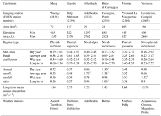
1In Verzasca, Allenbach and Riale die Calneggia there are some streamflow : rainfall ratios > 1 because the weather stations are located outside the catchment and precipitation is highly variable in alpine terrain.
2.1 HBV model
The HBV model was originally developed at the Hydrologiska Byråns Vattenbalansavdelning unit at the Swedish Meteorological and Hydrological Institute (SMHI) by Bergström (1976). The HBV model is a bucket-type model that represents snow, soil, groundwater and stream routing processes in separate routines. In this study, we used the version HBV-light (Seibert and Vis, 2012).
2.2 Catchments
The HBV-light model was set up for six 24–186 km2 catchments in Switzerland (Table 1 and Fig. 1). The catchments were selected based on the following criteria: (i) there is little anthropogenic influence, (ii) they are gauged at a single location, (iii) they have reliable streamflow data during high flow and low flow conditions (i.e. no complete freezing during winter and a cross section that allows accurate streamflow measurement at low flows) and (iv) there are no glaciers. The six selected catchments (Table 1) represent different streamflow regime types (Aschwanden and Weingartner, 1985). The snow-dominated highest elevation catchments (Allenbach and Riale di Calneggia) have the largest seasonality in streamflow, i.e. the biggest differences between the long-term maximum and minimum Pardé coefficients, followed by the rain- and snow-dominated Verzasca catchment. The rain-dominated catchments (Murg, Guerbe and Mentue) have the lowest seasonal variability in streamflow (Table 1). The mean elevation of the catchments varies from 652 to 2003 m a.s.l. (Table 1). The elevation range of each individual catchment was divided into 100 m elevation bands for the simulations.
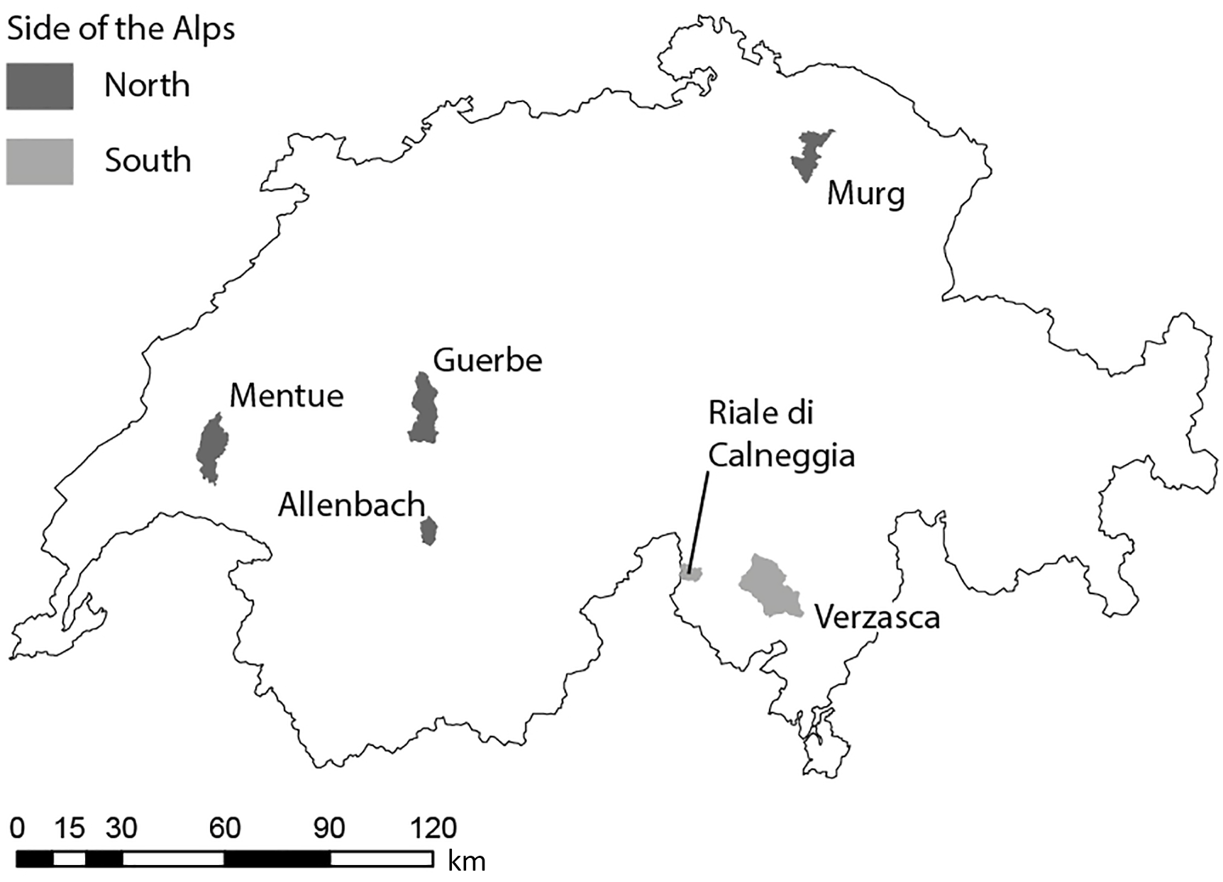
Figure 1Location of the six study catchments in Switzerland. Shading indicates whether the catchment is located on the north or south side of the Alps. See Table 1 for the characteristics of the study catchments.
2.3 Measured data
Hourly runoff time series (based on 10 min measurements) for the six study catchments were obtained from the Federal Office for the Environment (FOEN; see Table 1 for the gauging station numbers). The average hourly areal precipitation amounts were extracted for each study catchment from the gridded CombiPrecip dataset from MeteoSwiss (Sideris et al., 2014). This dataset combines gauge and radar precipitation measurements at an hourly timescale and 1 km2 spatial resolution and is available for the time period since 2005.
We used hourly temperature data from the automatic monitoring network of MeteoSwiss (see Table 1 for the stations) and applied a gradient of −6 ∘C per 1000 m to adjust the temperature of each weather station to the mean elevation of the catchment. Within the HBV model, the temperature was then adjusted for the different elevation bands using a calibrated lapse rate.
As recommended by Oudin et al. (2005), potential evapotranspiration was calculated using the temperature-based potential evapotranspiration model of McGuinness and Bordne (1972) using the day of the year, the latitude and the temperature. This rather simplistic approach was considered sufficient because this study focused on differences in model performance relative to a benchmark calibration.
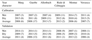
Table 2The calibration years (second most extreme and second closest to average years) and validation years (most extreme and closest to average years) for each catchment. The numbers in parentheses are the ranks over the period 1974–2014 (or 1990–2014 for Verzasca).
2.4 Selection of years for model calibration and validation
The model was calibrated for an average, a dry and a wet year to investigate the influence of wetness conditions and the amount of streamflow on the calibration results. The years were selected based on the total streamflow during summer (July–September). The driest and the wettest years of the period 2006–2014 were selected based on the smallest and largest sum of streamflow during the summer. The average streamflow years were selected based on the proximity to the mean summer streamflow for all the years 1974–2014 (1990–2014 for Verzasca). For each catchment the years that were the 2nd-closest to the mean summer streamflow for all years, as well as the years with the second lowest and second highest streamflow sum were chosen for model calibration (see Table 2). We did this separately for each catchment because for each catchment a different year was dry, average or wet. For the validation, we chose the year closest to the mean summer streamflow and the years with the lowest and the highest total summer streamflow (see Table 2). We used each of the parameter sets obtained from calibration for the dry, average or wet years to validate the model for each of the three validation years, resulting in nine validation combinations for each catchment (and each dataset, as described below).
2.5 Transformation of datasets to resemble citizen science data quality
2.5.1 Errors in crowdsourced streamflow observations
Strobl et al. (2018) asked 517 participants to estimate streamflow based on the stick method at 10 streams in Switzerland. Here we use the estimates for the medium-sized streams Töss, Sihl and Schanzengraben in the Canton of Zurich and the Magliasina in Ticino (n=136), which had a similar streamflow range at the time of the estimations (2.6–28 m3 s−1) as the mean annual streamflow of the six streams used for this study (1.2–10.8 m3 s−1). We calculated the streamflow from the estimated width, depth and flow velocities using a factor of 0.8 to adjust the surface flow velocity to the average velocity (Harrelson et al., 1994). The resulting streamflow estimates were normalised by dividing them by the measured streamflow. We then combined the normalised estimates of all four rivers and log-transformed the relative estimates. A normal distribution with a mean of 0.12 and a standard deviation of 1.30 fits the distribution of the log-transformed relative estimates well (standard error of the mean: 0.11, standard error of the standard deviation: 0.08; Fig. 2).
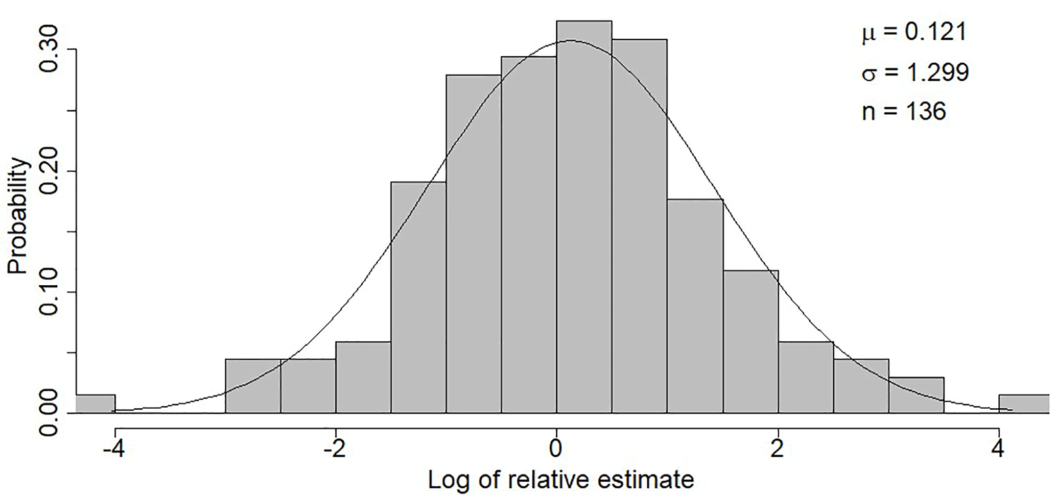
Figure 2Fit of the normal distribution to the frequency distribution of the log-transformed relative streamflow estimates (ratio of the estimated streamflow and the measured streamflow).
To create synthetic datasets with data quality characteristics that represent the observed crowdsourced streamflow estimates, we assumed that the errors in the streamflow estimates are uncorrelated (as they are likely provided by different people). For each time step, we randomly selected a relative error value from the log-normal distribution of the relative estimates (Fig. 2) and multiplied the measured streamflow with this relative error. To simulate the effect of training and to obtain time series with different data quality, two additional streamflow time series were created using a standard deviation divided by 2 (standard deviation of 0.65) and by 4 (standard deviation of 0.33). This reduces the spread in the data (but does not change the small systematic overestimation of the streamflow), so large outliers are still possible, but are less likely. To summarise, we tested the following four cases.
-
No error: the data measured by the FOEN, assumed to be (almost) error-free, the benchmark in terms of quality.
-
Small error: random errors according to the log-normal distribution of the snapshot campaigns with the standard deviation divided by 4.
-
Medium error: random errors according to the log-normal distribution of the surveys with the standard deviation divided by 2.
-
Large error: typical errors of citizen scientists, i.e. random errors according to the log-normal distribution of errors from the surveys.
2.5.2 Filtering of extreme outliers
Usually some form of quality control is used before citizen science data are analysed. Here, we used a very simple check to remove unrealistic outliers from the synthetic datasets. This check was based on the likely minimum and maximum streamflow for a given catchment area. We defined an upper limit of possible streamflow values as a function of the catchment area using the dataset of maximum streamflow from 1500 Swiss catchments provided by Scherrer AG, Hydrologie und Hochwasserschutz (2017). To account for the different precipitation intensities north and south of the Alps, different curves were created for the catchments on each side of the Alps. All streamflow observations, i.e. modified streamflow measurements, above the maximum observed streamflow for a particular catchment size including a 20 % buffer (Fig. S1), were replaced by the value of the maximum streamflow for a catchment of that size. This affected less than 0.5 % of all data points. A similar procedure was used for low flows based on a dataset of the FOEN with the lowest recorded mean streamflows over 7 days but this resulted in no replacements.
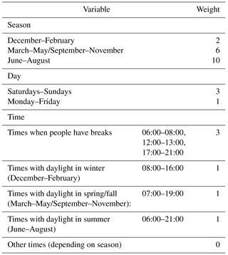
Table 3Weights assigned to specific seasons, days and times of the day for the random selection of data points for Crowd52 and Crowd12. The weights for each hour were multiplied and normalised. We then used them as probabilities for the individual hours. For times without daylight the probability was set to zero.
2.5.3 Temporal resolution of the observations
Data entries from citizen scientists are not as regular as data from sensors with a fixed temporal resolution. Therefore, we decided to test eight scenarios with a different temporal resolution and distribution of the data throughout the year to simulate different patterns in citizen contributions.
-
Hourly: one data point per hour (, depending on the year).
-
Weekly: one data point per week, every Saturday, randomly between 06:00 and 20:00 ().
-
Monthly: one data point per month on the 15th of the month, randomly between 06:00 and 20:00 (n=12).
-
IntenseSummer: one data point every other day from July until September, randomly between 06:00 and 20:00 (∼15 observations per month, n=46).
-
WeekendSummer: one data point each Saturday and each Sunday between May and October, randomly between 06:00 and 20:00 ().
-
WeekendSpring: one data point on each Saturday and each Sunday between March and August, randomly between 06:00 and 20:00 ().
-
Crowd52: 52 random data points during daylight (in order to be comparable to the Weekly, IntenseSummer, WeekendSummer and WeekendSpring time series).
-
Crowd12: 12 random data points during daylight (comparable to the Monthly data).
Except for the hourly data, these scenarios were based on our own experiences within the CrowdWater project (https://www.crowdwater.ch, last access: 3 October 2018) and information from the CrowdHydrology project (Lowry and Fienen, 2013). The hourly dataset was included to test the effect of errors when the temporal resolution of the data is optimal (i.e. by comparing simulations for the models calibrated with the hourly FOEN data and those calibrated with hourly data with errors). In the two scenarios Crowd52 and Crowd12, with random intervals between data points, we assigned higher probabilities for periods when people are more likely to be outdoors (i.e. higher probabilities for summer than winter, higher probabilities for weekends than weekdays, higher probabilities outside office hours; Table 3). Times without daylight (dependent on the season) were always excluded. We used the same selection of days, including the same times of the day for each of the four different error groups, years and catchments to allow comparison of the different model results.
2.6 Model calibration
For each of the 1728 cases (6 catchments, 3 calibration years, 4 error groups, 8 temporal resolutions), the HBV model was calibrated by optimising the overall consistency performance POA (Finger et al., 2011) using a genetic optimisation algorithm (Seibert, 2000). The overall consistency performance POA is the mean of four objective functions with an optimum value of 1: (i) NSE, (ii) the NSE for the logarithm of streamflow, (iii) the volume error and (iv) the mean absolute relative error (MARE). The parameters were calibrated within their typical ranges (see Table S1 in the Supplement.). To consider parameter uncertainty, the calibration was performed 100 times, which resulted in 100 parameter sets for each case. For each case, the preceding year was used for the warm-up period. For the Crowd52 and Crowd12 time series, we used 100 different random selections of times, whereas for the regularly spaced time series the same times were used for each case.
2.7 Model validation and analysis of the model results
The 100 parameters from the calibration for each case were used to run the model for the validation years (Table 2). For each case (i.e. each catchment, year, error magnitude and temporal resolution), we determined the median validation POA for the 100 parameter sets for each validation year. We analysed the validation results of all years combined and for all nine combinations of dry, mean and wet years separately.
Because the focus of this study was on the value of limited inaccurate streamflow observations for model calibration, i.e. the difference in the performance of the models calibrated with the synthetic data series compared to the performance of the models calibrated with hourly FOEN data, all model validation performances are expressed relative to the average POA of the model calibrated with the hourly FOEN data (our upper benchmark, representing the fully informed case when continuous high quality streamflow data are available). A relative POA of 1 indicates that the model performance is as good as the performance of the model calibrated with the hourly FOEN data, whereas lower POA values indicate a poorer performance.
In humid climates, the input data (precipitation and temperature) often dictate that model simulations can not be too far off as long as the water balance is respected (Seibert et al., 2018). To assess the value of limited inaccurate streamflow data for model calibration compared to a situation without any streamflow data, a lower benchmark (Seibert et al., 2018) was used. Here, the lower benchmark was defined as the median performance of the model ran with 1000 random parameters sets. By running the model with 1000 randomly chosen parameter sets, we represent a situation where no streamflow data for calibration are available and the model is driven only by the temperature and precipitation data. We used 1000 different parameter sets to cover most of the model variability due to the different parameter combinations. The Mann–Whitney U test was used to evaluate whether the median POA for a specific error group and temporal resolution of the data was significantly different from the median POA for the lower benchmark (i.e. the model runs with random parameters). We furthermore checked for differences in model performance for models calibrated with the same data errors but different temporal resolutions using a Kruskal–Wallis test. By applying a Dunn–Bonferroni post hoc test (Bonferroni, 1936; Dunn, 1959, 1961), we analysed which of the validation results were significantly different from each other.
The random generation of the 100 crowdsourced-like datasets (i.e. the Crowd52 and Crowd12 scenario) for each of the catchments and year characteristics resulted in time series with a different number of high flow estimates. In order to find out whether the inclusion of more high flow values resulted in a better validation performance, we defined the threshold for high flows as the streamflow value that was exceeded 10 % of the time in the hourly FOEN streamflow dataset. The Crowd52 and Crowd12 datasets were then divided into a group that had more than the expected 10 % high flow observations and a group that had fewer high flow observations. To determine if more high flow data improve model performance, the Mann–Whitney U test was used to compare the relative median POA of the two groups.
Table 4Median and the full range of the overall consistency performance POA scores for the upper benchmark (hourly FOEN data). The POA values for the dry, average and wet calibration years were used as the upper benchmarks for the evaluation based on the year character (Figs. 6 and S2 in the Supplement); the values in the “overall median” column were used as the benchmarks in the overall median performance evaluation shown in Fig. 4.
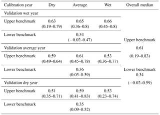
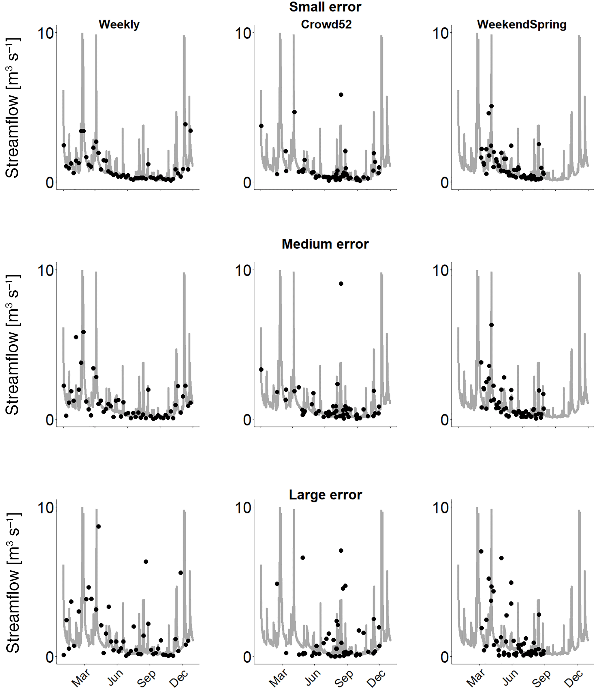
Figure 3Examples of streamflow time series used for calibration with small, medium and large errors and different temporal resolutions (Weekly, Crowd52 and WeekendSpring) for the Mentue in 2010. Large error: adjusted FOEN data with errors resulting from the log-normal distribution fitted to the streamflow estimates from citizen scientists (see Fig. 2). Medium error: same as large error, but the standard deviation of the log-normal distribution was divided by 2. Small error: same as the large error, but the standard deviation of the log-normal distribution was divided by 4. The grey line represents the measured streamflow, and the dots the derived time series of streamflow observations. Note that especially in the large error category some dots lie outside the figure margins.
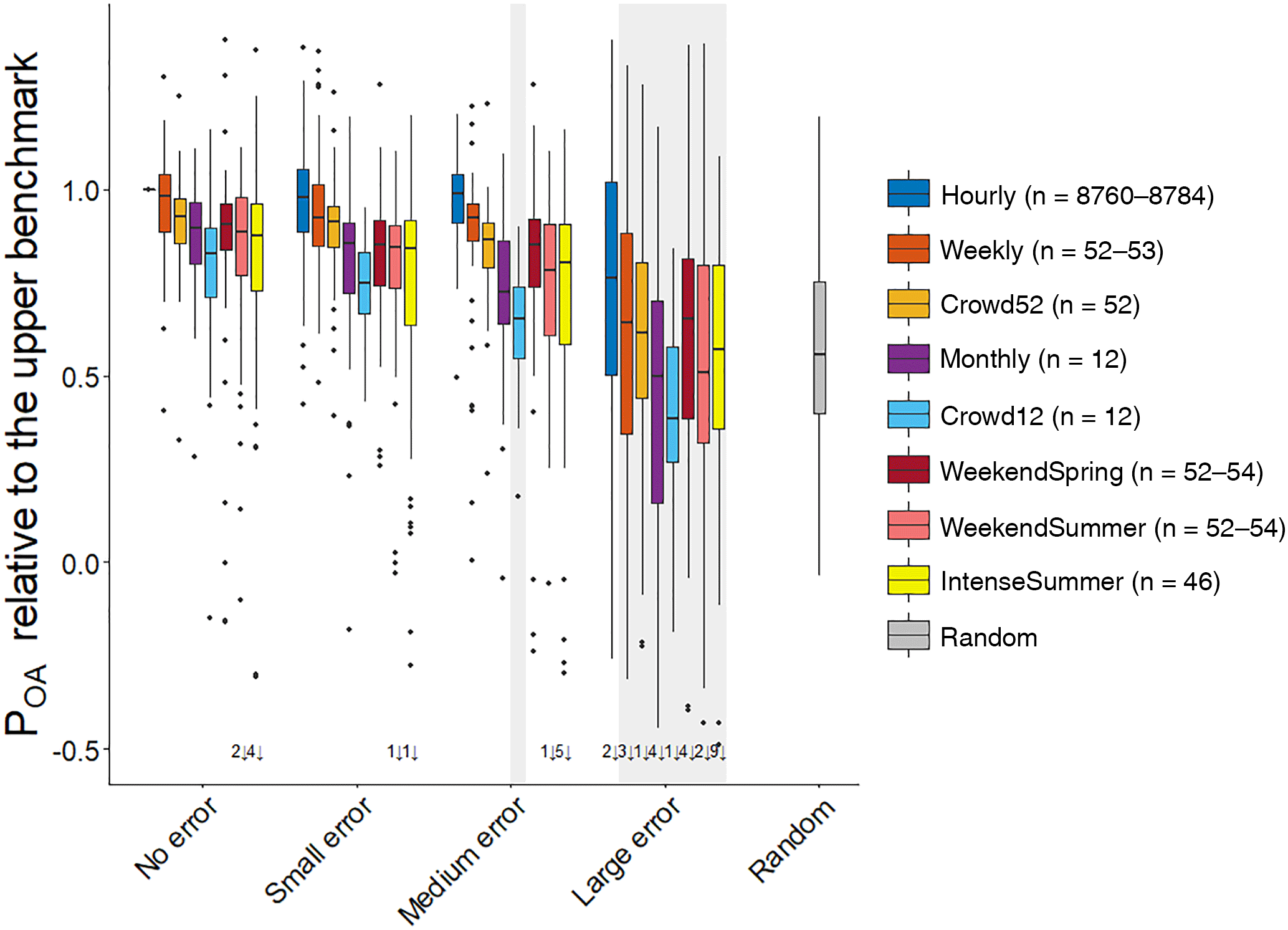
Figure 4Box plots of the median model performance relative to the upper benchmark for all datasets. The grey rectangles around the boxes indicate non-significant differences in median model performance compared to the lower benchmark with random parameter sets. The box represents the 25th and 75th percentile, the thick horizontal line represents the median, the whiskers extend to 1.5 times the interquartile range below the 25th percentile and above the 75th percentile and the dots represent the outliers. The numbers at the bottom indicate the number of outliers beyond the figure margins; n is the number of streamflow observations used for model calibration. The result of the hourly benchmark FOEN dataset has some spread because the results of the 100 parameters sets were divided by their median performance. A relative POA of 1 indicates that the model performance is as good as the performance of the model calibrated with the hourly FOEN data (upper benchmark).
3.1 Upper benchmark results
The model was able to reproduce the measured streamflow reasonably well when the complete and unchanged hourly FOEN datasets were used for calibration, although there were also a few exceptions. The average validation POA was 0.61 (range: 0.19–0.83; Table 4). The validation performance was poorest for the Guerbe (validation POA=0.19) because several high flow peaks were missed or underestimated by the model for the wet validation year. Similarly, the validation for the Mentue for the dry validation year resulted in a low POA (0.23) because a very distinct peak at the end of the year was missed and summer low flows were overestimated. The third lowest POA value was also for the Guerbe (dry validation year) but already had a POA of 0.35. Six out of the nine lowest POA values were for dry validation years. Validation for wet years for the models calibrated with data from wet years resulted in the best validation results (i.e. highest POA values; Table 4).
3.2 Effect of errors on the model validation results
Not surprisingly, increasing the errors in the streamflow data used for model calibration led to a decrease in the model performance (Fig. 4). For the small error category, the median validation performance was better than the lower benchmark for all temporal resolutions (Fig. 4 and Table S2). For the medium error category, the median validation performance was also better than the lower benchmark for all scenarios, except for the Crowd12 dataset. For the model calibrated with the dataset with large errors, only the Hourly dataset was significantly better than the lower benchmark (Table 5).
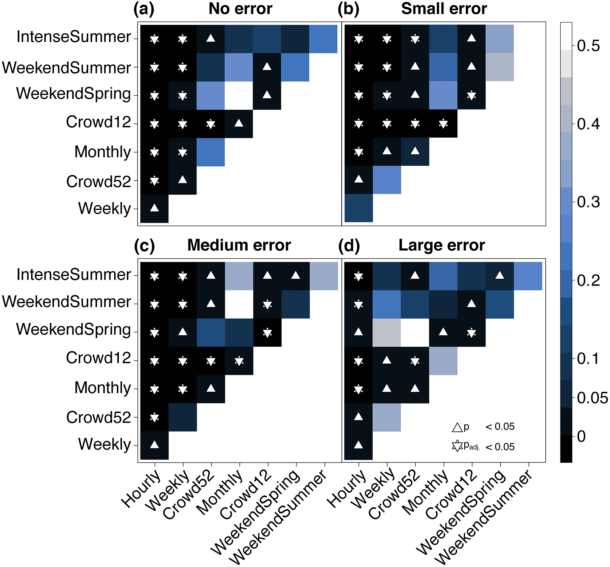
Figure 5Results (p values) of the Kruskal–Wallis with Bonferroni post hoc test to determine the significance of the difference in the median model performance for the data with different temporal resolutions within each data quality group (no error a, small error b, medium error c, and large error d). Blue shades represent the p values. White triangles indicate p values < 0.05 and white stars indicate p values that, when adjusted for multiple comparisons, are still < 0.05.
3.3 Effect of the data resolution on the model validation results
The Hourly measurement scenario resulted in the best validation performance for each error group, followed by the Weekly data, and then usually the Crowd52 data (Fig. 4). Although the median validation performance of the models calibrated with the Weekly datasets was better than for the Crowd52 dataset for all error cases, the difference was only statistically significant for the no error category (Fig. 5).
The validation performance of the models calibrated with the Weekly and Crowd52 datasets was better than for the scenarios focused on spring and summer observations (WeekendSpring, WeekendSummer and IntenseSummer). The median model performance for the Weekly dataset was significantly better than the datasets focusing on spring and summer for the no, small and medium error groups. The median performance of the Crowd52 dataset was only significantly better than all three measurement scenarios focusing on spring or summer for the small error case (Fig. 5). The model validation performance for the WeekendSummer and IntenseSummer scenarios decreased faster with increasing errors compared to the Weekly, Crowd52 or WeekendSpring datasets (Fig. 4). The median validation POA for the models calibrated with the WeekendSpring observations was better than for the models calibrated with the WeekendSummer and IntenseSummer datasets but the differences were only significant for the small, medium and large error groups. The differences in the model performance results for the observation strategies that focussed on summer (IntenseSummer and WeekendSummer) were not significant for any of the error groups (Fig. 5).
The median model performance for the regularly spaced Monthly datasets with 12 observations was similar to the median performance for the three datasets focusing on summer with 46–54 measurements (WeekendSpring, WeekendSummer and IntenseSummer), except for the case of large errors for which the monthly dataset performed worse. The irregularly spaced Crowd12 time series resulted in the worst model performance for each error group, but the difference from the performance for the regularly spaced Monthly data was only significant for the dataset with large errors (Fig. 5).

Figure 6Median model validation performance for the datasets calibrated and validated both in a dry year and in a wet year. Each horizontal line represents the median model performance for one catchment. The black bold line represents the median for the six catchments. The grey rectangles around the boxes indicate non-significant differences in median model performance for the six catchments compared to the lower benchmark with random parameters. The numbers at the bottom indicate the number of outliers beyond the figure margins. For the individual POA values of the upper benchmark (no error–Hourly dataset) in the different calibration and validation years, see Table 4.
3.4 Effect of errors and data resolution on the parameter ranges
For most parameters the spread in the optimised parameter values was smallest for the upper benchmark. The spread in the parameter values increased with increasing errors in the data used for calibration, particularly for MAXBAS (the routing parameter) but also for some other parameters (e.g. TCALT, TT and BETA). However, for some parameters (e.g. CFMAX, FC, and SFCF) the range in the optimised parameter values was mainly affected by the temporal resolution of the data and the number of data points used for calibration. It should be noted though that the changes in the range of model parameters differed significantly for the different catchments and the trends were not very clear.
3.5 Influence of the calibration and validation year and number of high flow data points on the model performance
The influence of the validation year on the model performance was larger than the effect of the calibration year (Figs. 6 and S2). In general model performance was poorest for the dry validation years. The model performances of all datasets with fewer observations or bigger errors than the Hourly datasets without errors were not significantly better than the lower benchmark for the dry validation years, except for Crowd52 in the no error group when calibrated with data from a wet year. However, even for the wet validation years some observation scenarios of the no error and small error group did not lead to significantly better model validation results compared to the median validation performance for the random parameters. Interestingly, the IntenseSummer dataset in the no error group resulted in a very good performance when the model was calibrated for a dry year and also validated in a dry year compared to its performance in the other calibration and validation year combinations. The median model performance was however not significantly better than the lower benchmark due to the low performance for the Guerbe and Allenbach (outliers beyond figure margins in Fig. 6). The validation results for these two catchments were the worst for all the no error–IntenseSummer datasets for all calibration and validation year combinations.
For 13 out of the 18 catchment and year combinations, the Crowd52 datasets with fewer than 10 % high streamflow data points led to a better validation performance than the Crowd52 datasets with more high streamflow data points. For six of them, the difference in model performance was significant. For none of the five cases where more high flow data points led to a better model performance was the difference significant. Also when the results were analysed by year character or catchment, there was no improvement when more high flow values were included in the calibration dataset.
4.1 Usefulness of inaccurate streamflow data for hydrological model calibration
In this study, we evaluated the information content of streamflow estimates by citizen scientists for calibration of a bucket-type hydrological model for six Swiss catchments. While the hydroclimatic conditions, the model or the calibration approach might be different in other studies, these results should be applicable for a wide range of cases. However, for physically based spatially distributed models that are usually not calibrated automatically, the use of limited streamflow data would probably benefit from a different calibration approach. Furthermore, our results might not be applicable in arid catchments where rivers become dry for some periods of the year because the linear reservoirs used in the HBV model are not appropriate for such systems.
Streamflow estimates by citizens are sometimes very different from the measured values, and the individual estimates can be disinformative for model calibration (Beven, 2016; Beven and Westerberg, 2011). The results show that if the streamflow estimates by citizen scientists were available at a high temporal resolution (hourly), these data would still be informative for the calibration of a bucket-type hydrological model despite their high uncertainties. However, observations with such a high resolution are very unlikely to be obtained in practice. All scenarios with error distributions that represent the estimates from citizen scientists with fewer observations were no better than the lower benchmark (using random parameters). With medium errors, however, and one data point per week on average or regularly spaced monthly data, the data were informative for model parameterisation. Reducing the standard deviation of the error distribution by a factor of 4 led to a significantly improved model performance compared to the lower benchmark for all the observation scenarios.
A reduction in the errors of the streamflow estimates could be achieved by training of citizen scientists (e.g. videos), improved information about feasible ranges for stream depth, width and velocity, or examples of streamflow values for well-known streams. Filtering of extreme outliers can also reduce the spread of the estimates. This could be done with existing knowledge of feasible streamflow values for a catchment of a given area or the amount of rainfall right before the estimate is made to determine if streamflow is likely to be higher or lower than for the previous estimate. More detailed research is necessary to test the effectiveness of such methods.
Le Coz et al. (2014) reported an uncertainty in stage–discharge streamflow measurements of around 5 %–20 %. McMillan et al. (2012) summarised streamflow uncertainties from stage–discharge relationships in a more detailed review and gave a range of ±50 %–100 % for low flows, ±10 %–20 % for medium or high (in-bank) flows and ±40 % for out-of-bank flows. The errors for the most extreme outliers in the citizen estimates are considerably higher, and could differ up to a factor of 10 000 from the measured value in the most extreme but rare cases (Fig. 2). Even with reduced standard deviations of the error distribution by a factor of 2 or 4, the observations in the most extreme cases can still differ by a factor of 100 and 10. The percentage of data points that differed from the measured value by more than 200 % was 33 % for the large error group, 19 % for the medium error group and 4 % for the small error group. Only 3 % of the data points were more than 90 % below the measured value in the large error group and 0 % for both in the medium and small error classes. If such observations are used for model calibration without filtering, they are seen as extreme floods or droughts, even if the actual conditions may be close to average flow. Beven and Westerberg (2011) suggest isolating periods of disinformative data. It is therefore beneficial to identify such extreme outliers, independent of a model, e.g. with knowledge of feasible maximum and minimum streamflow quantities, as used in this study, with the help of the maximum regionalised specific streamflow values for a given catchment area.
4.2 Number of streamflow estimates required for model calibration
In general, one would assume that the calibration of a model becomes better when there are more data (Perrin et al., 2007), although others have shown that the increase in model performance plateaus after a certain number of measurements (Juston et al., 2009; Pool et al., 2017; Seibert and Beven, 2009; Seibert and McDonnell, 2015). In this study, we limited the length of the calibration period to 1 year because in practice it may be possible to obtain a limited number of measurements during a 1-year period for ungauged catchments before the model results are needed for a certain application, as has been assumed in previous studies (Pool et al., 2017; Seibert and McDonnell, 2015). While a limited number of observations (12) was informative for model calibration when the data uncertainties were limited, the results of this study also suggest that the performance of bucket-type models decreases faster with increasing errors when fewer data points are available (i.e. there was a faster decline in model performance with increasing errors for models calibrated with 12 data points than for the models calibrated with 48–52 data points). This finding was most pronounced when comparing the model performance for the small and medium error groups (Fig. 4). These findings can be explained by the compensating effect of the number of observations and their accuracy because the random errors for the inaccurate data average out when a large number of observations are used, as long as the data do not have a large bias.
4.3 Best timing of streamflow estimates for model calibration
The performance of the parameter sets depended on the timing and the error distribution of the data used for model calibration. The model performance was generally better if the observations were more evenly spread throughout the year. For example, for the cases of no and small errors, the performance of the model calibrated with the Monthly dataset with 12 observations was better than for the IntenseSummer and WeekendSummer scenarios with 46–54 observations. Similarly, the less clustered observation scenarios performed better than the more clustered scenarios (i.e. Weekly vs. Crowd52, Monthly vs. Crowd12, Crowd52 vs. IntenseSummer, etc.). This suggests that more regularly distributed data over the year lead to a better model calibration. Juston et al. (2009) compared different subsamples of hydrological data for a 5.6 km2 Swedish catchment and found that including inter-annual variability in the data used for the calibration of the HBV model reduced the model uncertainties. More evenly distributed observations throughout the year might represent more of the within-year streamflow variability and therefore result in improved model performance. This is good news for using citizen science data for model calibration as it suggests that the timing is not as important as the number of observations because it is likely much easier to get observations throughout the year than during specific periods or flow conditions.
When comparing the WeekendSpring, WeekendSummer and IntenseSummer datasets, it seems that it was in most cases more beneficial to include data from spring rather than summer. This tendency was more pronounced with increasing data errors. The reason for this might be that the WeekendSpring scenario includes more snowmelt or rain-on-snow event peaks, in addition to usually higher baseflow, and therefore contains more information on the inter-annual variability in streamflow.
By comparing different variations of 12 data points to calibrate the HBV model, Pool et al. (2017) found that a dataset that contains a combination of different maximum (monthly, yearly etc.) and other flows in model calibration led to the best model performance but also that the differences in performance for the different datasets covering the range of flows were small. In our study we did not specifically focus on the high or low flow data points, and therefore did not have datasets that contained only high flow estimates, which would be very difficult to obtain with citizen science data. However, our findings similarly show that for model calibration for catchments with seasonal variability in streamflow it is beneficial to obtain data for different magnitudes of flow. Furthermore, we found that data points during relatively dry periods are beneficial for validation or prediction in another year and might even be beneficial for years with the same characteristics, as was shown for the improved validation performance of the IntenseSummer dataset compared to the other datasets when data from dry years were used for calibration (Fig. 6).
4.4 Effects of different types of years on model calibration and validation
The calibration year, i.e. the year in which the observations were made, was not decisive for the model performance. Therefore, a model calibrated with data from a dry year can still be useful for simulations for an average or wet year. This also means that data in citizen science projects can be collected during any year and that these data are useful for simulating streamflow for most years, except the driest years. However, model performance did vary significantly for the different validation years. The results during dry validation years were almost never significantly better than the lower benchmark (Fig. S2). This might be due to the objective function that was used in this study. Especially the NSE was lower for dry years because the flow variance (i.e. the denominator in the equation) is smaller when there is a larger variation in streamflow. Also, these results are based on six median model performances, and therefore, outliers have a big influence on the significance of results (Fig. S2).
Lidén and Harlin (2000) used the HBV-96 model by Lindström et al. (1997) with changes suggested by Bergström et al. (1997) for four catchments in Europe, Africa and South America. They achieved better model results for wetter catchments and argued that during dry years evapotranspiration plays a bigger role and therefore the model performance is more sensitive to inaccuracies in the simulation of the evapotranspiration processes. The fact that we used a very simple method to calculate the potential evapotranspiration (McGuinness and Bordne, 1972) might also explain why the model performed less well during dry years.
The model parameterisation, obtained from calibration using the IntenseSummer dataset, resulted in a surprisingly good performance for the validation for a more extreme dry year for four out of the six catchments. For the two catchments for which the performance for the IntenseSummer dataset was poor (Guerbe and Allenbach), the weather stations are located outside the catchment boundaries. Especially during dry periods missed streamflow peaks due to misrepresentation of precipitation can affect model performance a lot. The fact that always one of these two catchments had the worst model performance for all the no error–IntenseSummer runs furthermore indicates that the July–September period might not be suitable to represent characteristic runoff events for these catchments. The bad performance for these two catchments for the IntenseSummer–no error run with calibration and validation in the dry year resulted in the insignificant improvement in model performance compared to the lower benchmark. Because the wetness of a year was based on the summer streamflow, these findings suggest that data obtained during times of low flow result in improved validation performance during dry years compared to data collected during other times (Fig. S2). This suggests that if the interest is in understanding the streamflow response during very dry years, it is important to obtain data during the dry period. To test this hypothesis, more detailed analyses are needed.
4.5 Recommendations for citizen science projects
Our results show that streamflow estimates from citizens are not informative for hydrological model calibration, unless the errors in the estimates can be reduced through training or advanced filtering of the data to reduce the errors (i.e. to reduce the number of extreme outliers). In order to make streamflow estimates useful, the standard deviation of the error distribution of the estimates needs to be reduced by a factor of 2. Gibson and Bergman (1954) suggest that errors in distance estimates can be reduced from 33 % to 14 % with very little training. These findings are encouraging, although their tests covered distances larger than 365 m (400 yards) and the widths of the medium-sized rivers for which the streamflow was estimated were less than 40 m (Strobl et al., 2018). Options for training might be tutorial videos, as well as lists with values for the width, average depth and flow velocity of well-known streams (Strobl et al., 2018). In order to determine the effect of training on streamflow estimates, further research has to be done because especially the depth estimates were inaccurate (Strobl et al., 2018).
The findings of this study suggest the following recommendations for citizen science projects that want to use streamflow estimates:
-
Collect as many data points as possible. In this study hourly data always led to the best model performance. It is therefore beneficial to collect as many data points as possible. Because it is unlikely that hourly data are obtained, we suggest to aim for (on average) one observation per week. Provided that the standard deviation of the streamflow estimates can be reduced by a factor of 2, 52 observations (as in the Crowd52 data series) are informative for model calibration. Therefore, it is essential to invest in advertisement of a project and to find suitable locations where many people can potentially contribute, as well as to communicate to the citizen scientists that it is beneficial to submit observations regularly.
-
Encourage observations throughout the year. To further improve the model performance, or to allow for greater errors, it is beneficial to have observations at all types of flow conditions during the year, rather than during a certain season.
Observations during high streamflow conditions were in most cases not more informative than flows during other times of the year. Efforts to ask citizens to submit observations during specific flow conditions (e.g. by sending reminders to the citizen observers) do not seem to be very effective in light of the above findings. It is rather more beneficial to remind them to submit observations regularly.
Instead of focussing on training to reduce the errors in the streamflow estimates, an alternative approach for citizen science projects is to switch to a parameter that is easier to estimate, such as stream levels (Lowry and Fienen, 2013). Recent studies successfully used daily stream-level data (Seibert and Vis, 2016) and stream-level class data (van Meerveld et al. 2017) to calibrate hydrological models, and other studies have demonstrated the potential value of crowdsourced stream level data for providing information on, e.g. baseflow (Lowry and Fienen, 2013), or for improving flood forecasts (Mazzoleni et al., 2017). However, further research is needed to determine if real crowdsourced stream-level (class) data are informative for the calibration of hydrological models.
The results of this study extend previous studies on the value of limited hydrological data for hydrological model calibration or the best timing of streamflow measurements for model calibration (Juston et al., 2009; Pool et al., 2017; Seibert and McDonnell, 2015) that did not consider observation errors. This is an important aspect, especially when considering citizen science approaches to obtain streamflow data. Our results show that inaccurate streamflow data can be useful for model calibration, as long as the errors are not too large. When the distribution of errors in the streamflow data represented the distribution of the errors in the streamflow estimates from citizen scientists, this information was not informative for model calibration (i.e. the median performance of the models calibrated with these data was not significantly better than the median performance of the models with random parameter values). However, if the standard deviation of the estimates is reduced by a factor of 2, then the (less) inaccurate data would be informative for model calibration. We furthermore demonstrated that realistic frequencies for citizen science projects (one observation on average per week or month) can be informative for model calibration. The findings of studies such as the one presented here provide important guidance on the design of citizen science projects as well as other observation approaches.
The data are available from FOEN (streamflow) and MeteoSwiss (precipitation and temperature). The HBV software is available at https://www.geo.uzh.ch/en/units/h2k/Services/HBV-Model.html (Seibert and Vis, 2012) or from jan.seibert@geo.uzh.ch.
The supplement related to this article is available online at: https://doi.org/10.5194/hess-22-5243-2018-supplement.
While JS and IvM had the initial idea, the concrete study design was based on input from all authors. SE and BS conducted the field surveys to determine the typical errors in streamflow estimates. The simulations and analyses were performed by SE. The writing of the manuscript was led by SE; all co-authors contributed to the writing.
The authors declare that they have no conflict of interest.
We thank all citizen scientists who participated in the field surveys, as
well as the Swiss Federal Office for the Environment for providing the
streamflow data, MeteoSwiss for providing the weather data, Maria Staudinger,
Jan Schwanbeck and Scherrer AG for the permission to use their datasets and
the reviewers for the useful comments. This project was funded by the Swiss
National Science Foundation (project CrowdWater).
Edited by: Nadav Peleg
Reviewed by: two
anonymous referees
Aschwanden, H. and Weingartner, R.: Die Abflussregimes der Schweiz, Geographisches Institut der Universität Bern, Abteilung Physikalische Geographie, Gewässerkunde, Bern, Switzerland, 1985.
Bergström, S.: Development and application of a conceptual runoff model for Scandinavian catchments, Sveriges Meteorologiska och Hydrologiska Institut (SMHI), Norrköping, Sweden, available at: https://www.researchgate.net/publication/255274162_Development_and_Application_of_a_Conceptual_Runoff_Model_for_Scandinavian_Catchments (last access: 3 October 2018), 1976.
Bergström, S., Carlsson, B., Grahn, G., and Johansson, B.: A More Consistent Approach to Watershed Response in the HBV Model, Vannet i Nord., 4, 1997.
Beven, K.: Facets of uncertainty: epistemic uncertainty, non-stationarity, likelihood, hypothesis testing, and communication, Hydrol. Sci. J., 61, 1652–1665, https://doi.org/10.1080/02626667.2015.1031761, 2016.
Beven, K. and Westerberg, I.: On red herrings and real herrings: disinformation and information in hydrological inference, Hydrol. Process., 25, 1676–1680, https://doi.org/10.1002/hyp.7963, 2011.
Bonferroni, C. E.: Teoria statistica delle classi e calcolo delle probabilità, st. Super. di Sci. Econom. e Commerciali di Firenze, Istituto superiore di scienze economiche e commerciali, Florence, Italy, 62 pp., 1936.
Brath, A., Montanari, A., and Toth, E.: Analysis of the effects of different scenarios of historical data availability on the calibration of a spatially-distributed hydrological model, J. Hydrol., 291, 232–253, https://doi.org/10.1016/j.jhydrol.2003.12.044, 2004.
Buytaert, W., Zulkafli, Z., Grainger, S., Acosta, L., Alemie, T. C., Bastiaensen, J., De BiÃv̈re, B., Bhusal, J., Clark, J., Dewulf, A., Foggin, M., Hannah, D. M., Hergarten, C., Isaeva, A., Karpouzoglou, T., Pandeya, B., Paudel, D., Sharma, K., Steenhuis, T., Tilahun, S., Van Hecken, G., and Zhumanova, M.: Citizen science in hydrology and water resources: opportunities for knowledge generation, ecosystem service management, and sustainable development, Front. Earth Sci., 2, 21 pp., https://doi.org/10.3389/feart.2014.00026, 2014.
Davids, J. C., van de Giesen, N., and Rutten, M.: Continuity vs. the Crowd – Tradeoffs Between Continuous and Intermittent Citizen Hydrology Streamflow Observations, Environ. Manage., 60, 12–29, https://doi.org/10.1007/s00267-017-0872-x, 2017.
Davids, J. C., Rutten, M. M., Shah, R. D. T., Shah, D. N., Devkota, N., Izeboud, P., Pandey, A., and van de Giesen, N.: Quantifying the connections – linkages between land-use and water in the Kathmandu Valley, Nepal, Environ. Monit. Assess., 190, 17 pp., https://doi.org/10.1007/s10661-018-6687-2, 2018.
Dickinson, J. L., Zuckerberg, B., and Bonter, D. N.: Citizen Science as an Ecological Research Tool: Challenges and Benefits, Annu. Rev. Ecol. Evol. Syst., 41, 149–172, https://doi.org/10.1146/annurev-ecolsys-102209-144636, 2010.
Dunn, O. J.: Estimation of the Medians for Dependent Variables, Ann. Math. Stat., 30, 192–197, https://doi.org/10.1214/aoms/1177706374, 1959.
Dunn, O. J.: Multiple Comparisons among Means, J. Am. Stat. Assoc., 56, 52–64, https://doi.org/10.1080/01621459.1961.10482090, 1961.
Ewen, T., Brönnimann, S., and Annis, J.: An extended Pacific-North American index from upper-air historical data back to 1922, J. Climate, 21, 1295–1308, https://doi.org/10.1175/2007JCLI1951.1, 2008.
Finger, D., Pellicciotti, F., Konz, M., Rimkus, S., and Burlando, P.: The value of glacier mass balance, satellite snow cover images, and hourly discharge for improving the performance of a physically based distributed hydrological model, Water Resour. Res., 47, 14 pp., https://doi.org/10.1029/2010WR009824, 2011.
Finger, D., Vis, M., Huss, M., and Seibert, J.: The value of multiple data set calibration versus model complexity for improving the performance of hydrological models in mountain catchments, Water Resour. Res., 51, 1939–1958, https://doi.org/10.1002/2014WR015712, 2015.
Fitzner, D., Sester, M., Haberlandt, U., and Rabiei, E.: Rainfall Estimation with a Geosensor Network of Cars – Theoretical Considerations and First Results, Photogramm. Fernerkun., 2013, 93–103, https://doi.org/10.1127/1432-8364/2013/0161, 2013.
Gibson, E. J. and Bergman, R.: The effect of training on absolute estimation of distance over the ground, J. Exp. Psychol., 48, 473–482, https://doi.org/10.1037/h0055007, 1954.
Haberlandt, U. and Sester, M.: Areal rainfall estimation using moving cars as rain gauges – a modelling study, Hydrol. Earth Syst. Sci., 14, 1139–1151, https://doi.org/10.5194/hess-14-1139-2010, 2010.
Harrelson, C. C., Rawlins, C. L., and Potyondy, J. P.: Stream channel reference sites: an illustrated guide to field technique, Department of Agriculture, Forest Service, Rocky Mountain Forest and Range Experiment Station location, Fort Collins, CO, US, 1994.
Horner, I., Renard, B., Le Coz, J., Branger, F., McMillan, H. K., and Pierrefeu, G.: Impact of Stage Measurement Errors on Streamflow Uncertainty, Water Resour. Res., 54, 1952–1976, https://doi.org/10.1002/2017WR022039, 2018.
Juston, J., Seibert, J., and Johansson, P.: Temporal sampling strategies and uncertainty in calibrating a conceptual hydrological model for a small boreal catchment, Hydrol. Process., 23, 3093–3109, https://doi.org/10.1002/hyp.7421, 2009.
Koch, J. and Stisen, S.: Citizen science: A new perspective to advance spatial pattern evaluation in hydrology, PLoS One, 12, 1–20, https://doi.org/10.1371/journal.pone.0178165, 2017.
Le Coz, J., Renard, B., Bonnifait, L., Branger, F., and Le Boursicaud, R.: Combining hydraulic knowledge and uncertain gaugings in the estimation of hydrometric rating curves: A Bayesian approach, J. Hydrol., 509, 573–587, https://doi.org/10.1016/j.jhydrol.2013.11.016, 2014.
Lidén, R. and Harlin, J.: Analysis of conceptual rainfall–runoff modelling performance in different climates, J. Hydrol., 238, 231–247, https://doi.org/10.1016/S0022-1694(00)00330-9, 2000.
Lindström, G., Johansson, B., Persson, M., Gardelin, M., and Bergström, S.: Development and test of the distributed HBV-96 hydrological model, J. Hydrol., 201, 272–288, https://doi.org/10.1016/S0022-1694(97)00041-3, 1997.
Lowry, C. S. and Fienen, M. N.: CrowdHydrology: Crowdsourcing Hydrologic Data and Engaging Citizen Scientists, Ground Water, 51, 151–156, https://doi.org/10.1111/j.1745-6584.2012.00956.x, 2013.
Mazzoleni, M., Verlaan, M., Alfonso, L., Monego, M., Norbiato, D., Ferri, M., and Solomatine, D. P.: Can assimilation of crowdsourced data in hydrological modelling improve flood prediction?, Hydrol. Earth Syst. Sci., 21, 839–861, https://doi.org/10.5194/hess-21-839-2017, 2017.
McGuinness, J. and Bordne, E.: A comparison of lysimeter-derived potential evapotranspiration with computed values, Agricultural Research Service – United States Department of Agriculture Location, Washington D.C., 1972.
McMillan, H., Freer, J., Pappenberger, F., Krueger, T., and Clark, M.: Impacts of uncertain river flow data on rainfall-runoff model calibration and discharge predictions, Hydrol. Process., 24, 1270–1284, https://doi.org/10.1002/hyp.7587, 2010.
McMillan, H., Krueger, T., and Freer, J.: Benchmarking observational uncertainties for hydrology: rainfall, river discharge and water quality, Hydrol. Process., 26, 4078–4111, https://doi.org/10.1002/hyp.9384, 2012.
Michel, C., Perrin, C., and Andreassian, V.: The exponential store: a correct formulation for rainfall – runoff modelling, Hydrol. Sci. J., 48, 109–124, https://doi.org/10.1623/hysj.48.1.109.43484, 2003.
Oudin, L., Hervieu, F., Michel, C., Perrin, C., Andréassian, V., Anctil, F., and Loumagne, C.: Which potential evapotranspiration input for a lumped rainfall-runoff model?, J. Hydrol., 303, 290–306, https://doi.org/10.1016/j.jhydrol.2004.08.026, 2005.
Perrin, C., Michel, C., and Andréassian, V.: Improvement of a parsimonious model for streamflow simulation, J. Hydrol., 279, 275–289, https://doi.org/10.1016/S0022-1694(03)00225-7, 2003.
Perrin, C., Ouding, L., Andreassian, V., Rojas-Serna, C., Michel, C., and Mathevet, T.: Impact of limited streamflow data on the efficiency and the parameters of rainfall-runoff models, Hydrol. Sci. J., 52, 131–151, https://doi.org/10.1623/hysj.52.1.131, 2007.
Pool, S., Viviroli, D., and Seibert, J.: Prediction of hydrographs and flow-duration curves in almost ungauged catchments: Which runoff measurements are most informative for model calibration?, J. Hydrol., 554, 613–622, https://doi.org/10.1016/j.jhydrol.2017.09.037, 2017.
Ruhi, A., Messager, M. L., and Olden, J. D.: Tracking the pulse of the Earth's fresh waters, Nat. Sustain., 1, 198–203, https://doi.org/10.1038/s41893-018-0047-7, 2018.
Scherrer AG: Verzeichnis grosser Hochwasserabflüsse in schweizerischen Einzugsgebieten, Auftraggeber: Bundesamt für Umwelt (BAFU), Abteilung Hydrologie, Reinach, 2017.
Seibert, J.: Multi-criteria calibration of a conceptual runoff model using a genetic algorithm, Hydrol. Earth Syst. Sci., 4, 215–224, https://doi.org/10.5194/hess-4-215-2000, 2000.
Seibert, J. and Beven, K. J.: Gauging the ungauged basin: how many discharge measurements are needed?, Hydrol. Earth Syst. Sci., 13, 883–892, https://doi.org/10.5194/hess-13-883-2009, 2009.
Seibert, J. and McDonnell, J. J.: Gauging the Ungauged Basin?: Relative Value of Soft and Hard Data, J. Hydrol. Eng., 20, A4014004-1–6, https://doi.org/10.1061/(ASCE)HE.1943-5584.0000861, 2015.
Seibert, J. and Vis, M. J. P.: Teaching hydrological modeling with a user-friendly catchment-runoff-model software package, Hydrol. Earth Syst. Sci., 16, 3315–3325, https://doi.org/10.5194/hess-16-3315-2012, 2012.
Seibert, J. and Vis, M. J. P.: How informative are stream level observations in different geographic regions?, Hydrol. Process., 30, 2498–2508, https://doi.org/10.1002/hyp.10887, 2016.
Seibert, J., Vis, M. J. P., Lewis, E., and van Meerveld, H. J.: Upper and lower benchmarks in hydrological modelling, Hydrol. Process., 32, 1120–1125, https://doi.org/10.1002/hyp.11476, 2018.
Shiklomanov, A. I., Lammers, R. B., and Vörösmarty, C. J.: Widespread decline in hydrological monitoring threatens Pan-Arctic Research, Eos, Trans. Am. Geophys. Union, 83, 13–17, https://doi.org/10.1029/2002EO000007, 2002.
Sideris, I. V., Gabella, M., Erdin, R., and Germann, U.: Real-time radar-rain-gauge merging using spatio-temporal co-kriging with external drift in the alpine terrain of Switzerland, Q. J. Roy. Meteor. Soc., 140, 1097–1111, https://doi.org/10.1002/qj.2188, 2014.
Strobl, B., Etter, S., van Meerveld, I., and Seibert, J.: Accuracy of Crowdsourced Streamflow and Stream Level Class Estimates, Hydrol. Sci. J., (special issue on hydrological data: opportunities and barriers), in review, 2018.
van Meerveld, H. J. I., Vis, M. J. P., and Seibert, J.: Information content of stream level class data for hydrological model calibration, Hydrol. Earth Syst. Sci., 21, 4895–4905, https://doi.org/10.5194/hess-21-4895-2017, 2017.
Vrugt, J. A., Gupta, H. V., Dekker, S. C., Sorooshian, S., Wagener, T., and Bouten, W.: Application of stochastic parameter optimization to the Sacramento Soil Moisture Accounting model, J. Hydrol., 325, 288–307, https://doi.org/10.1016/j.jhydrol.2005.10.041, 2006.
Weeser, B., Stenfert Kroese, J., Jacobs, S. R., Njue, N., Kemboi, Z., Ran, A., Rufino, M. C., and Breuer, L.: Citizen science pioneers in Kenya – A crowdsourced approach for hydrological monitoring, Sci. Total Environ., 631–632, 1590–1599, https://doi.org/10.1016/j.scitotenv.2018.03.130, 2018.
Yapo, P. O., Gupta, H. V., and Sorooshian, S.: Automatic calibration of conceptual rainfall-runoff models: sensitivity to calibration data, J. Hydrol., 181, 23–48, https://doi.org/10.1016/0022-1694(95)02918-4, 1996.