the Creative Commons Attribution 4.0 License.
the Creative Commons Attribution 4.0 License.
 | 15 Oct 2018
Rainfall disaggregation for hydrological modeling: is there a need for spatial consistence?
Hannes Müller-Thomy
Markus Wallner
Kristian Förster
In this study, the influence of disaggregated rainfall products with different degrees of spatial consistence on rainfall–runoff modeling results is analyzed for three mesoscale catchments in Lower Saxony, Germany. For the disaggregation of daily rainfall time series into hourly values, a multiplicative random cascade model is applied. The disaggregation is applied on a station by station basis without consideration of surrounding stations; hence subsequent steps are then required to implement spatial consistence. Spatial consistence is represented here by three bivariate spatial rainfall characteristics that complement each other. A resampling algorithm and a parallelization approach are evaluated against the disaggregated time series without any subsequent steps. With respect to rainfall, clear differences between these three approaches can be identified regarding bivariate spatial rainfall characteristics, areal rainfall intensities and extreme values. The resampled time series lead to the best agreement with the observed ones. Using these different rainfall products as input to hydrological modeling, we hypothesize that derived runoff statistics – with emphasis on seasonal extreme values – are subject to similar differences as well. However, an impact on the extreme values' statistics of the hydrological simulations forced by different rainfall approaches cannot be detected. Several modifications of the study design using rainfall–runoff models with and without parameter calibration or using different rain gauge densities lead to similar results in runoff statistics. Only if the spatially highly resolved rainfall–runoff WaSiM model is applied instead of the semi-distributed HBV-IWW model can slight differences regarding the seasonal peak flows be identified. Hence, the hypothesis formulated before is rejected in this case study. These findings suggest that (i) simple model structures might compensate for deficiencies in spatial representativeness through parameterization and (ii) highly resolved hydrological models benefit from improved spatial modeling of rainfall.
- Article
(6947 KB) -
Supplement
(958 KB) - BibTeX
- EndNote


Flood quantiles are important information for the creation of flood hazard maps, the construction of riverfront buildings and landscape development plans, for example. For ungauged catchments and catchments with short discharge observation periods, rainfall–runoff modeling is a possibility to obtain long, simulated discharge time series which can then be used for derived flood frequency analysis.
The most important data input for rainfall–runoff modeling are rainfall time series (Beven, 2001). Melsen et al. (2016) gave an overview of typical processes for different catchment sizes and corresponding temporal resolutions. For catchments with areas of a few hundred square kilometers, time series with hourly resolutions are required for the simulation of instantaneous flood peaks. In most of these cases, observed rainfall time series of that kind are (i) too short or (ii) the network density is too low. Both are issues because (i) limits the length of the simulation period and hence the derivable flood frequencies and (ii) affects the representation of spatial rainfall patterns (Krajewski et al., 1991; Ogden and Julien, 1993; Obled et al., 1994, and Nicotina et al., 2008) and hence the areal rainfall used as input for the rainfall–runoff simulations.
Usually, time series of daily stations have much longer observation periods and a higher network density. Daily time series can be disaggregated to hourly time series by using information from observed, hourly time series. One possible method for the disaggregation of rainfall is the multiplicative random cascade model (e.g., Olsson, 1998), which was originally introduced within the field of turbulence theory (Mandelbrot, 1974). The use of observed daily time series as input is a strong advantage of the cascade model, since starting with “true” rainfall amounts and intermittency facilitates their conservation to finer temporal resolutions, while other rainfall generators (e.g., Poisson cluster models; Rodriguez-Iturbe et al., 1987; Onof et al., 2000) try to generate time series with a certain temporal resolution and target statistics without any temporal reference to observations.
With the microcanonical cascade model, the rainfall amount of a coarse time step (e.g., a day) is conserved exactly through the disaggregation process, so that an aggregation of the disaggregated time series would result exactly in the original observed time series. Starting from a daily resolution, an hourly temporal resolution is achieved, which is a convenient input resolution for many rainfall–runoff models. However, this disaggregation method is a univariate process, carried out for single time series only which are independent of the time series of surrounding stations. Through the systematically random distribution of the rainfall amount within a day, unrealistic patterns of rainfall are generated and the spatial consistence of rainfall is missing. If an unrealistic spatial distribution of rainfall is used within a rainfall–runoff simulation, it can be assumed that this affects the simulated runoff. However, a realistic spatial representation of rainfall is essential if the time series serve as input for rainfall–runoff modeling (e.g., Gires et al., 2015; Paschalis et al., 2014; Ochoa-Rodriguez et al., 2015; Peleg et al., 2017).
Müller and Haberlandt (2015) have introduced a resampling scheme as a subsequent step after the disaggregation process, which can be used for the implementation of spatial consistence within disaggregated time series. Spatial consistence is hereby defined by three bivariate rainfall characteristics: the probability of occurrence, Pearson's coefficient of correlation and the continuity ratio (Wilks, 1998). The implementation of spatial consistence for hourly time series was proven by the abovementioned bivariate characteristics in addition to areal rainfall intensities resulting from the disaggregated time series. Without resampling, areal rainfall intensities were underestimated. The resampling algorithm was additionally tested for time series of 5 min resolution by Müller and Haberlandt (2018). Bivariate rainfall characteristics as well as the simulated runoff from an artificial sewage system were positively validated against observed rainfall time series and its resulting simulated runoff.
Haberlandt and Radtke (2014) overcame the lack of spatial consistence using a parallelization approach, which leads to an overestimation of simulated floods, but is preferred in comparison to a possible underestimation. However, Ding et al. (2016) also used disaggregated time series for their rainfall–runoff analyses with a focus on instantaneous peak flows, but without any subsequent changes to the disaggregated time series. Neither a systematic over- or underestimation of simulated discharge and flood peaks can be found in both investigations.
It can be questioned why the simulation results from both studies, both based upon unrealistic spatial rainfall behavior, lead to an acceptable representation of observed discharge characteristics. The hypothesis of this study is that rainfall products with different degrees of spatial consistence will result in different areal rainfall intensities and hence influence runoff statistics derived from simulated runoff time series. Therefore, three different rainfall products are used as input for rainfall–runoff modeling: disaggregated time series with (Müller and Haberlandt, 2015) and without (Ding et al., 2016) the implementation of spatial consistence, and thirdly, time series with an “overestimated spatial consistence” by parallelization (Haberlandt and Radtke, 2014). A systematic comparison is carried out including rainfall–runoff simulations with and without calibration, differing station densities and different rainfall–runoff models.
In general, calibration and validation of rainfall–runoff model parameters are carried out through a quantitative comparison of simulated and observed time series. This strategy is not applicable using disaggregated rainfall time series as input, since the daily rainfall amount is distributed randomly in time during a day. Hence, the temporal connection between rainfall and runoff is missing. An alternative strategy is the calibration on runoff statistics and has been applied before by others, for example, Yu and Yang (2000), Westerberg et al. (2011), Haberlandt and Radtke (2014), Wallner and Haberlandt (2015) and Ding et al. (2016). Runoff statistics are time-independent, but contain useful information about the hydrograph and hence about the hydrological regime and its characteristics. It is assumed that, by a simultaneous consideration of different complimentary runoff statistics, the runoff behavior can be represented sufficiently. Possible runoff statistics are runoff extremes for different seasons of a year (to take into account, e.g., summer and winter floods with their different geneses and resulting runoff behavior), flow duration curves (to describe the overall behavior) and average monthly values (to describe the interannual variability).
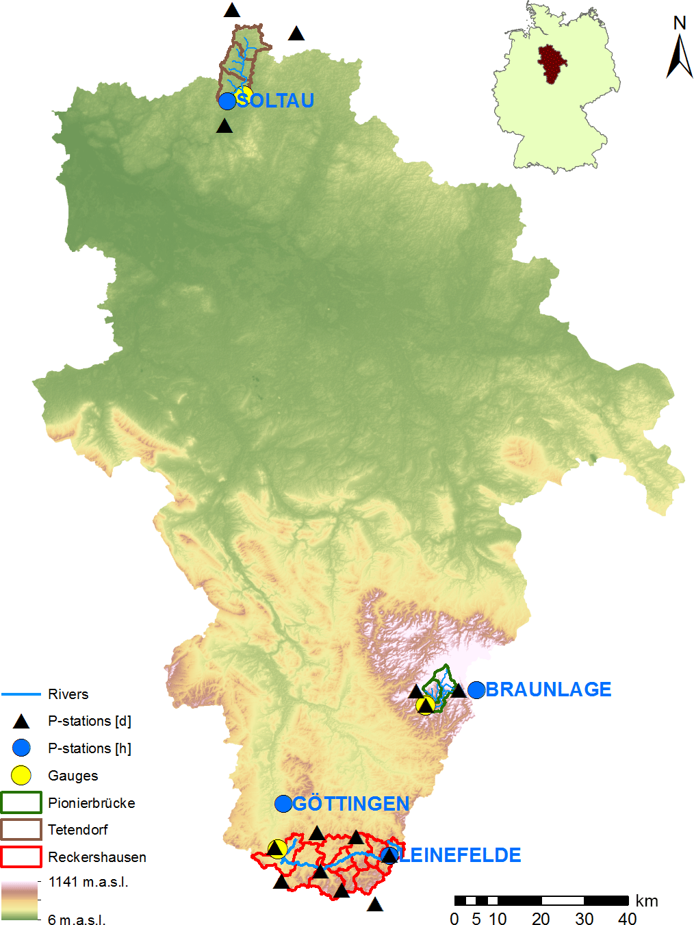
Figure 1Location of all three catchments in the Aller–Leine river basin and its location in Germany.
The paper is organized as follows: after a brief description of the study area and the data in Sect. 2, the rainfall generation including the implementation of spatial consistence and the applied rainfall–runoff models including the calibration technique are explained in Sect. 3. Section 4 includes the results for both the rainfall generation and rainfall–runoff modeling. A summary of the rainfall–runoff model results is provided in Sect. 5 and general conclusions and a brief outlook are provided in Sect. 6.
2.1 Catchments
The investigation is carried out for three catchments in the Aller–Leine river basin, namely Reckershausen, Pionierbrücke and Tetendorf (see Fig. 1). The river basin is situated in Lower Saxony, Northern Germany, and has been investigated regarding its runoff extreme values before (e.g., Haberlandt and Radtke, 2014; Ding et al., 2016; Fangmann and Haberlandt, 2018). Based on the Köppen–Geiger climate classification, the river basin can be divided into a temperate oceanic climate in the north and a temperate continental climate in the south (Peel et al., 2007). For Reckershausen an additional investigation regarding rain gauge network density is carried out. All hourly and daily stations for Reckershausen are shown in Fig. 2.
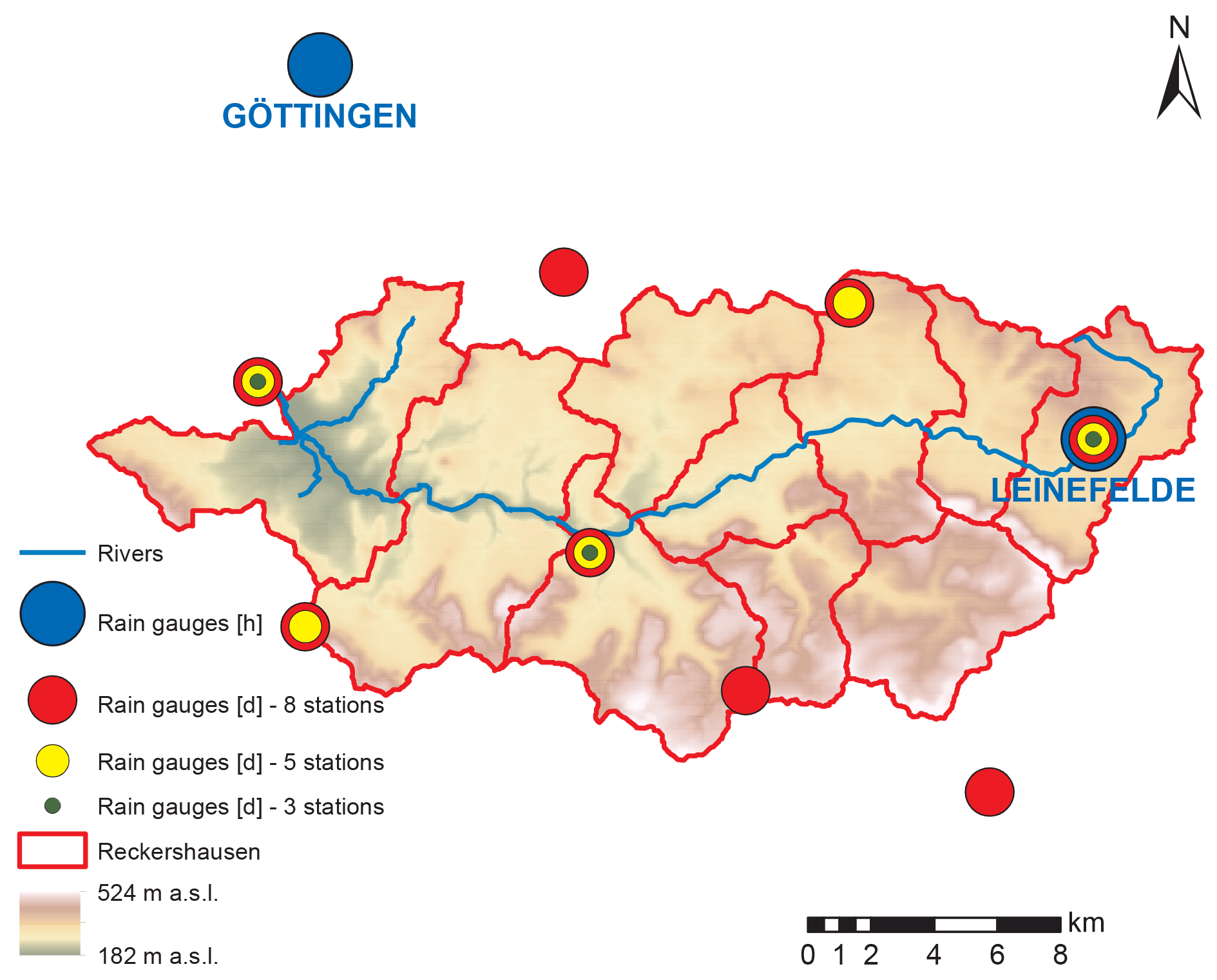
Figure 2Reckershausen catchment including sets of three, five and eight daily stations used for network density analysis.
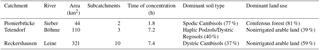
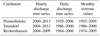
The catchments differ concerning area and elevation as well as land use and soil conditions. A brief description can be found in Table 1. The soil information is extracted from the soil map BÜK1000 of the Federal Republic of Germany with a scale of 1 : 1 000 000 (Hartwich et al., 1998). Information regarding the land use is extracted from the CORINE database (Federal Environment Agency, 2009). The time of concentration has been estimated as per Kirpich (1940).
Table 1Brief description of the investigated catchments with percentages of dominant soil type and land use.
2.2 Climate data
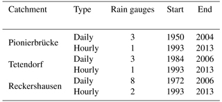
For the rainfall disaggregation, time series of hourly and daily stations are required. Time series of the hourly stations are used for the parameter estimation of the cascade model (described in Sect. 3.1a), which is in turn used for the disaggregation of the time series of the daily stations. An overview of rain gauges used in this study is given in Fig. 1, while their measuring periods are given in Table 2. For the daily stations, the chosen period is the longest available period with data for all stations in a catchment. From Table 2 it can be seen that time series have a longer duration for daily stations in comparison to those for hourly stations for all catchments (up to 2.7 times for Pionierbrücke). Additionally, the number of daily stations is higher.
Table 2Rain gauges and time series lengths used for each catchment.
For the rainfall–runoff model HBV (see Sect. 3.2), time series of precipitation, temperature and potential evaporation are needed. The following description of data processing of temperature and potential evaporation is based on Wallner et al. (2013) and was carried out for the whole Aller–Leine basin. The temperature time series were derived through an interpolation using external drift kriging of 38 hourly stations with hourly resolution, whereby the additional information is elevation.
The calculation of the potential evaporation is carried out using the Turc–Wendling method on a daily basis (DVWK, 1996). The required sunshine duration per day was derived through ordinary kriging using 29 stations. To achieve an hourly resolution, daily values have been divided by 24, since the inter-daily distribution of potential evaporation has been shown not to be that sensitive as model input. Different land use types have been taken into account by using an average land use parameter (DVWK, 2002) similar to the crop coefficient. All input data were interpolated and subsequently aggregated to subcatchment scale.
For the WaSiM model, which is only applied for the Pionierbrücke catchment, climate time series are needed as point or gridded information on an hourly basis. From the Braunlage climate station, time series of temperature, relative air humidity and wind speed are available with an hourly resolution. Global radiation was only available on a daily basis, but has been disaggregated to hourly values using an approach as in Förster et al. (2016).
2.3 Runoff data
The available discharge data of the three catchments are listed in Table 3. While observed hourly time series have only been available since 2000 (Pionierbrücke) and 2004 (Tetendorf and Reckershausen), observed extreme values exist for much longer periods. Daily discharge time series exist for at least as long as the period of the hourly extreme values on a monthly basis.
For the calibration, a special focus is given to the extreme values of the summer (1 May–31 October) and winter period (1 November–30 April). Therefore, the maximum observed value of each half year was extracted from both data sources, observed hourly time series and monthly extreme values, to generate periods as long as possible.
The method section consists of two subsections. In Sect. 3.1, the multiplicative cascade model for the disaggregation of rainfall time series is explained. Additionally, two methods for the implementation of spatial consistence in the disaggregated time series are presented. The descriptions of the two rainfall–runoff models HBV and WaSiM and the calibration procedure for HBV can be found in Sect. 3.2.
3.1 Rainfall generation
(a) Rainfall disaggregation
The multiplicative random cascade model (Müller and Haberlandt, 2015) is applied for the disaggregation of time series of the daily stations. A general scheme of this model is shown in Fig. 3. One coarse time step is divided into b finer time steps of equal length. The branching number b determines the number of finer time steps and is in the first disaggregation time step b=3 and in all following disaggregation steps down to 1 h resolution b=2. The cascade model is microcanonical, so the rainfall amount of each time step is conserved exactly. A re-aggregation of the disaggregated time series yields the observed time series used for the disaggregation. Since the focus of this study is not on the disaggregation itself, the interested reader is referred to Müller and Haberlandt (2015) for a more detailed explanation. However, the main results are a slight underestimation of dry spell duration (relative error of −6 %), percentage of dry intervals (−3 %), wet spell duration (−12 %) and amount (−9 %), while average intensity is slightly overestimated (4 %). While the autocorrelation function also shows underestimations, the extreme values are represented well.

Figure 3General disaggregation scheme of the applied multiplicative cascade model (values inside the boxes represent rainfall amount, and a blue or white box color indicates wet or dry time steps, respectively).
(b) Bivariate characteristics
For the definition of spatial consistence applied in this study, the bivariate rainfall characteristics follow the ones used by Haberlandt et al. (2008) and are briefly described in the following.
The probability of occurrence Pk,l describes the probability of rainfall occurrence at the same time at two stations k and l:
where n is the total number of non-missing observation hours at both stations, zi is the rainfall intensity and the number of simultaneous rainfall occurrence at both stations is represented by n11.
Pearson's coefficient of correlation ρ describes the relationship between simultaneously occurring rainfall at two stations k and l as a measure of the linear relation between both rainfall time series (Eq. 2). Breinl et al. (2014) used this coefficient before for multisite rainfall generation:
Müller and Haberlandt (2015) found an intensity dependency for Pearson's coefficient of correlation and distinguished between ρ(k≤4 mm) and ρ(k>4 mm), which is adopted here.
The continuity ratio Ck, l compares the expected rainfall amount at one station for times with and without rain at the neighboring station (E is the expectation operator):
These characteristics are distance-dependent and prescribed values can be estimated as functions of the separation distance between two stations from observed data (see regression lines in Fig. 4 for each characteristic).
(c) Implementation of spatial consistence
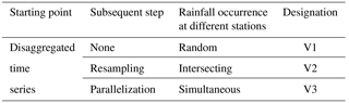
As mentioned before, the disaggregation of single time series is a point process with no surrounding stations taken into account. Input rainfall products for the rainfall–runoff models consisting of just the disaggregated time series without subsequent steps to implement spatial consistence are referred to as V1 (no implementation of spatial consistence). Two methods for the implementation of spatial consistence, and resulting in the rainfall products V2 and V3, are applied in this study.
The first method, resulting in V2, is based on simulated annealing (Aarts and Korst, 1965; Kirkpatrick et al., 1983), a nonlinear optimization method from the group of resampling algorithms. The aim of simulated annealing is to modify the disaggregated time series and in doing so minimize an objective function including the deviations between the observed bivariate rainfall characteristics and those from the disaggregated time series. Relative diurnal cycles are swapped without changing the structure of the time series or the absolute daily totals of rainfall amounts. The interested reader is referred to Müller and Haberlandt (2015) for further details.

Figure 4Bivariate spatial rainfall characteristics of V1, V2 and V3 in comparison to observations for the Pionierbrücke catchment (for one realization, black circles represent observations – for details the reader is referred to Müller and Haberlandt, 2015).
The second method, resulting in rainfall product V3, is a more pragmatic solution. It was introduced by Haberlandt and Radtke (2014) and is also based on the time series of V1 that is already disaggregated. For each day, the station with the highest rainfall amount is identified. The relative diurnal cycle of this station is transferred to all other stations for this day. This parallelization is carried out for all days of the disaggregated time series. The varying diurnal distributions of rainfall at each station without spatial patterns, leading to an underestimation of spatial consistence, are transformed instead to a simultaneous occurrence of rainfall at all stations with an overestimation of spatial consistence.
Both methods are compared against using the disaggregated time series without any subsequent steps. For analyses and discussion of the impacts of these methods, the designations listed in the summarizing Table 4 are used.
3.2 Hydrological models
For analyzing the impact of rainfall products with different spatial consistencies, two models, HBV-IWW (Wallner et al., 2013) and WaSiM (Schulla, 1997, 2015), are used. All simulations are carried out continuously. This enables the derivation of flood frequency analyses and avoids uncertainties from unknown initial conditions resulting from event-based modeling (Pathiraja et al., 2012). Additionally, an initial phase of 1 year is used as a spin-up period to achieve plausible initial conditions for all storages.
(a) HBV-IWW including calibration procedure
The HBV-IWW model is based on the HBV model that was originally developed at the Swedish Meteorological and Hydrological Institute (SMHI) in the early 1970s (Bergström, 1976) and was modified by Wallner et al. (2013). HBV-IWW, denoted HBV for simplification, is a conceptual model, whereby runoff generation and runoff transformation are represented by simple relationships between storage and effective precipitation, or runoff (see flowchart of the model in Fig. S1 in the Supplement). For the spatial discretization of the study areas, subcatchments (see Fig. 2) with an approx. area of 20 km2 are applied. It could be questioned whether a rainfall–runoff model with subcatchments is useful for the validation of the spatial consistence of rainfall. A daily station covers an area of 65 km2 on average in Germany (Müller, 2016). This spatial resolution is not increased by the cascade model in this study, since only a temporal disaggregation is applied. Also, no additional information is gained by a model with higher spatial resolution. So the only disadvantage could be a sort of numerical diffusion due to the spatial resolution. However, since subcatchments of this size are used throughout a number of studies, the HBV with this spatial resolution represents the state of the art and is applied for the current study.
For the estimation of the areal rainfall of each subcatchment, a two-step approach was chosen. First, rainfall is interpolated with a nearest neighbor approach on a raster basis with cell widths of 1 km. In the second step, areal rainfall for each subcatchment is calculated through the arithmetic mean of all raster cells within the subcatchment. If the areal rainfall of a subcatchment is dominated by one station, it could be questioned whether areal rainfall intensities should be reduced (by, e.g., areal reduction factors; Sivapalan and Blöschl, 1998; Veneziano and Langousis; 2005; Wright et al., 2013) to avoid an overestimation (e.g., Peleg et al., 2018). Since underestimations also occur in the continuous simulation if this station was not in the center of the storm, no areal reduction was carried out.
Snow accumulation and snowmelt are based on a threshold temperature and the degree day method. After snow storage, all precipitation and snowmelt enters the soil storage where actual evaporation is considered. Depending on the state of the soil storage, water is released to the upper groundwater layer from where surface runoff and interflow can occur. Both are controlled by a storage coefficient. Water from the upper groundwater layer can also percolate to the lower groundwater layer. The outflow from the latter represents the baseflow component. Surface runoff, interflow and baseflow are finally summarized and transformed via a triangular unit hydrograph. River routing is carried out via the Muskingum method. Further details about the model parameters can be found in Wallner et al. (2013) and in Table S2 in the Supplement.
For the calibration, the following runoff statistics are used: quantiles of the distribution functions fitted to the extreme values of (i) summer (Extr-Su, May to October) and (ii) winter (Extr-Wi, November to April), (iii) quantiles of the flow duration curve (FDC) and (iv) monthly averages (Q-mon). The calibration is carried out for each rainfall product separately, but for all 10 realizations at the same time (resulting in 1 parameter set for 10 realizations) The calibration procedure is also illustrated in Fig. S1.
For Extr-Su and Extr-Wi, a two-parametric Gumbel distribution is fitted to the annual series of extreme values. L moments are used for parameter estimation to reduce the sensitivity against outliers (Hosking and Wallis, 1997). Although extreme values only occur in a few time steps, their reproduction in the discharge time series is the main aim of the simulation on an hourly basis. However, since the extreme values only represent a small fraction of the discharge time series, FDC and Q-mon are also used to represent the more frequent discharge values. Q-mon accounts for the temporal dependency on the interannual variation of the discharge. The analyses of FDC and Q-mon allow no direct validation of the rainfall products, but enable an overall plausible simulation of rainfall–runoff processes. Hence, FDC and Q-mon are calculated from averaged daily discharge values in order to reduce computation time. For the goodness-of-fit analyses of simulated (Sim) and observed (Obs) statistics, the Nash–Sutcliffe-efficiency, NSE (Nash and Sutcliffe, 1970), is used. A perfect fit would result in NSE = 1, while assuming the average of the observed data for all time steps would result in NSE = 0. The equation for the NSE is given in Eq. (4) and the corresponding quantiles for Extr-Su, Extr-Wi and FDC and months for the Q-mon, respectively, are given in Eq. (5).
The goodness-of-fit values of all runoff statistics are summarized in the objective function Ostat, which should be minimized during the calibration:
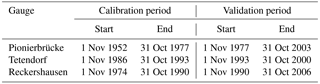
For the optimization, simulated annealing is used. The parameters modified during the optimization with the corresponding ranges are given in Table S2. The periods for calibration and validation are listed in Table 5 for each catchment.
(b) WaSiM
WaSiM (Schulla, 1997, 2015) is a physically based and distributed hydrological model which has been designed to study climate change and land use change impacts on the water balance and floods in mesoscale catchments (e.g., Niehoff et al., 2002; Bormann and Elfert, 2010). WaSiM was formerly known as WaSiM-ETH, but has since been renamed (Schulla, 2015), and hence the new abbreviation is used throughout the paper. WaSiM is flexible regarding the resolution of spatial input data. In general, elevation, land use and soil data need to be prepared as gridded raster datasets. The spatial resolution of WaSiM applications covers several scales ranging from tens of meters to a few kilometers. For this study a spatial resolution of 150 m×150 m was chosen.
For the areal rainfall estimation, a combined inverse distance weighting and elevation-dependent regression approach is applied. This approach does not only account for a horizontal interpolation but also addresses the typically observed increase in precipitation with increasing elevation, which proves helpful given that the catchment spans an altitudinal range of several hundred meters.
A set of alternative hydrological process representations for each of the following sub-models is included in the model in order to cover different user needs and meteorological data requirements: (i) evapotranspiration, (ii) snow, (iii) interception and (iv) soil water. This list is not exhaustive since other processes can also be addressed using the model. Here, only the processes utilized in this study are described. Potential evapotranspiration is computed using the Penman–Monteith approach (e.g., Monteith, 1965), taking look-up tables of parameters defined for different land use classes into account. Seasonal snow cover dynamics is simulated using a temperature threshold for phase partitioning and a temperature index model for snowmelt calculations. A bucket approach is applied to consider interception of rainwater. The soil water dynamics including actual evapotranspiration, infiltration, lateral outflow (interflow) and percolation is simulated in a numerical scheme which is based on the Richards equation. The lowermost nodes in each grid cell, which are subject to saturation, represent the groundwater storage in the model. A linear storage approach is applied here to simulate the outflow from the groundwater.
Since WaSiM is more complex than HBV with respect to computational needs, a different strategy for model calibration was chosen. As the number of both adjustable parameters and iterations is limited due to limited computational resources, a lexicographical approach was set up for model calibration (Gelleszun et al., 2017). In this way, the optimization of parameters is divided into subsequent steps that are associated with different processes. In a first step, the parameters of the soil water balance and runoff generation (i.e., recession of hydraulic conductivity along the soil profile and the flow density) have been calibrated through maximizing NSE. Then, the baseflow recession is improved through minimizing the root mean square error of the lowermost part of the flow duration curve (two parameters). Both calibration steps have been performed using hourly meteorological time series and observed discharge time series from the period 2009–2012. As highly resolved meteorological observations are only available from 2000 onwards, an additional calibration step has been carried out using disaggregated rainfall time series in order to better match the long-term water balance characteristics through slightly modifying canopy resistance parameters of the evapotranspiration model. Without these pre-calibration steps an underestimation of the mean discharge and hence the water balance was identified. An incorrect representation of the water balance introduces other uncertainty sources, which hence superpose the effects of the different versions of spatial rainfall. However, this pre-calibration was only focused on the water balance itself and not on the objectives used in Eq. (6).
For the discussion of the results, the section is divided into two parts. The first part deals with the interpretation of the rainfall spatial variability, while the influence on simulated discharges is discussed in the second part.
4.1 Rainfall
For the disaggregation of daily rainfall time series to hourly values, the microcanonical cascade model of Müller and Haberlandt (2015) is used. This model was previously validated in the aforementioned study for the Aller–Leine river basin, which is also considered in this study. Since the focus of this study is the spatial variability of the generated rainfall, the interested reader is referred to their investigation for a detailed analysis of point results. In Fig. 4 the bivariate characteristics are shown for V1, V2 and V3 in comparison with the observations for Pionierbrücke (results for the other two catchments are in Fig. S3 and S4). For the V1 case (the disaggregated time series without any subsequent steps), the probability of occurrence and the correlation coefficients are underestimated, whereas the continuity ratio is overestimated.
For the V2 case, the probability of occurrence and the correlation coefficients could be improved. While values for the probability of occurrence and correlation coefficient for rainfall intensities >4 mm are similar to observations, a slight underestimation can be identified for correlation coefficients for rainfall intensities ≤4 mm for some station pairs. For the continuity ratio, V2 results vary. This is due to the definition of the criterion, taking station k with respect to station l into account, but not vice versa. This definition leads to different values for the same station pair because different time steps are taken into account. Therefore, for Ck, l an improvement can be identified during simultaneous worsening of Cl, k.
It should be noted that the resampling algorithm has not been validated in the context of distances smaller than 20 km for hourly time steps. Although the spatial rainfall characteristics are underestimated after the disaggregation (V1), a major improvement for all characteristics can be identified by the application of V2, moving all station pairs into the cloud of observations (except some of the continuity ratio).
The simultaneous rainfall of V3 leads to the best values for the continuity ratio, comparable to those from observations. However, slight overestimations can be identified for both coefficients of correlation. For the probability of occurrence, high overestimations can be identified (approximately 50 %). Although the same diurnal cycles are used for all stations, the probability of occurrence is less than 1 due to the fact that rainfall does not necessarily occur at all stations on a wet day.
Additionally, the influence of the spatial consistence on resulting areal rainfall intensities is investigated. In the Supplement S5, areal rainfall intensities resulting from V1, V2 and V3 are shown for one subcatchment of Pionierbrücke. Since only one observed high-resolution time series (Reckershausen: two) is available for each catchment, no comparison between areal rainfall intensities between observed and disaggregated time series (resulting from three stations for each catchment) can be carried out. Areal rainfall intensities resulting from disaggregated time series can only be compared among each other. V1 leads to the lowest rainfall intensities, V3 to the highest. Areal rainfall intensities of V2 lie between V1 and V3. The “random” rainfall occurrence in V1 leads to smaller rainfall intensity values as was indicated by the probability of occurrence (see Fig. 4). Accordingly, the parallelization of V3 leads to the highest areal rainfall intensities. Therefore, the results for the spatial bivariate characteristics and the areal rainfall intensities are consistent. The findings are similar for the other subcatchments in Tetendorf and Reckershausen.
Additionally, the extreme values of the areal rainfall intensities have been analyzed, since those can have a significant influence on the resulting runoff. In Fig. 5, the annual maxima rainfall extremes for another subcatchment in Pionierbrücke are illustrated using the Weibull plotting position (similar for all subcatchments). As identified for all areal rainfall intensities, for the extreme values, V1 also leads to the lowest values for each return period. V2 and V3 result in similar values regarding the mean for all return periods. The clear difference of higher values for V3 over the whole spectrum of non-exceedance probability cannot be identified for the extreme values (see Fig. S5). However, for V3, where the diurnal cycle of the station with the highest daily rainfall amount is transferred to the time series of all other stations, V3 does not lead to the highest extreme values. The reason for this is that the highest daily rainfall amount does not necessarily lead to the highest rainfall intensity on the final disaggregation level with an hourly time step. As an example, a rainfall station A with a daily total rainfall amount of 50 mm has a maximum intensity during this day of 8 mm h−1, whereas station B with a daily total rainfall of 40 mm has a higher maximum intensity of 15 mm h−1. As such, V3 can also lead to a smoothing of the rainfall intensities, at least for peak intensities. So for return periods 1.5 years years, V2 even results in the highest rainfall extremes. However, for higher return periods (>20 years), V3 leads to higher range of extreme values and higher extreme values itself than V2.
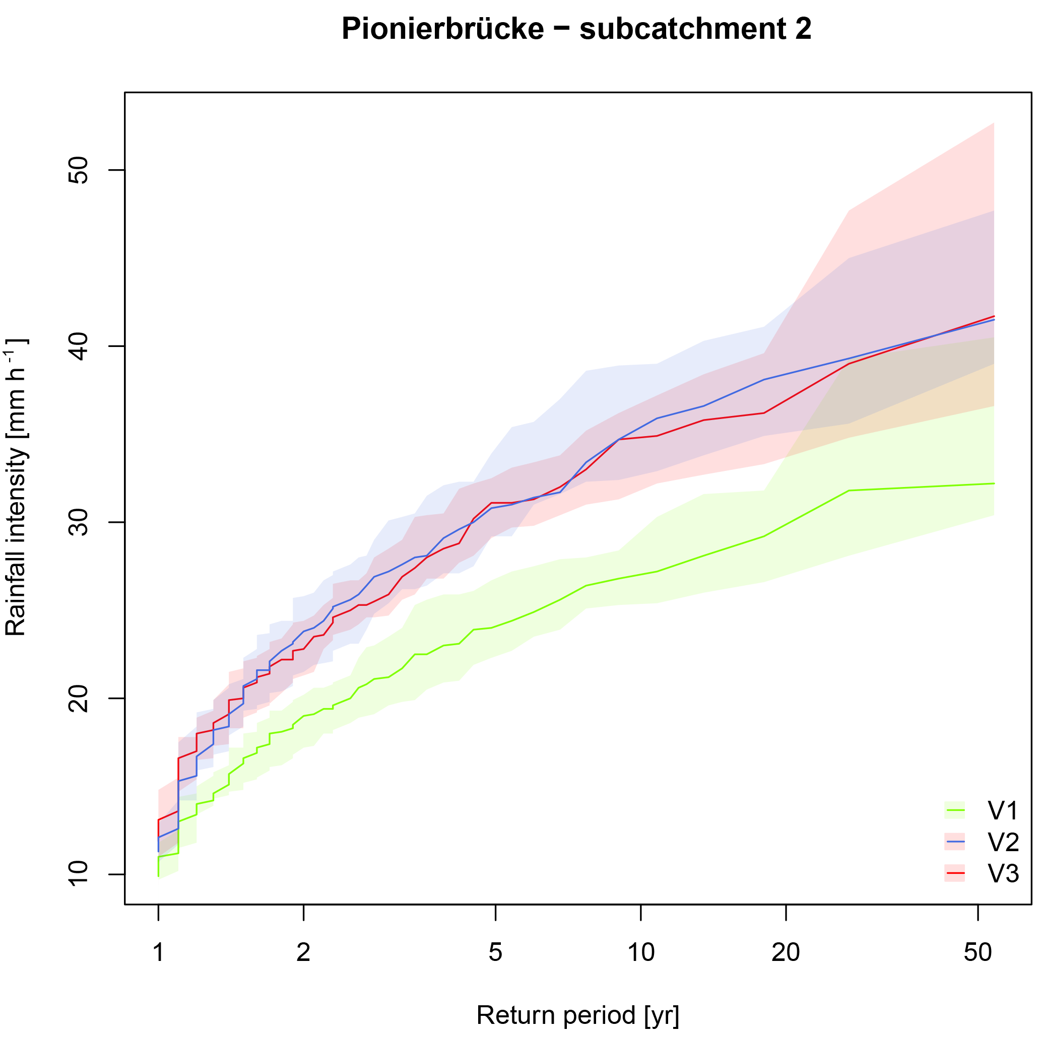
Figure 5Annual rainfall extremes of the areal rainfall intensities for subcatchment 2 in Pionierbrücke. For all 10 realizations used as input for HBV, the solid line represents the median (based on annual extreme values from 1 November 1950 to 31 October 2003).
It can be summarized that V1, V2 and V3 lead to different results regarding spatial characteristics and areal rainfall intensities.
4.2 Rainfall–runoff model results
In this section, all rainfall–runoff simulation results are presented. The section is organized as follows: in (a) the rainfall–runoff model results using HBV are shown for all catchments for V1, V2 and V3 with three rain gauges as input for each. In (b) HBV model results for different station densities for the Reckershausen catchment are presented. HBV model results without parameter calibration are shown for all catchments in (c), while WaSiM model results are presented in (d) for the Pionierbrücke catchment. As mentioned before, the focus of this study is on seasonal extreme values of runoff, Extr-Su and Extr-Wi. The cumulative runoff statistics Q-mon and FDC are additionally applied to train and validate the hydrological model not only for extreme events, which might have led to implausible parameter sets, not representing the general behavior of the catchment.
(a) HBV simulation results with calibration using three rain gauges as input
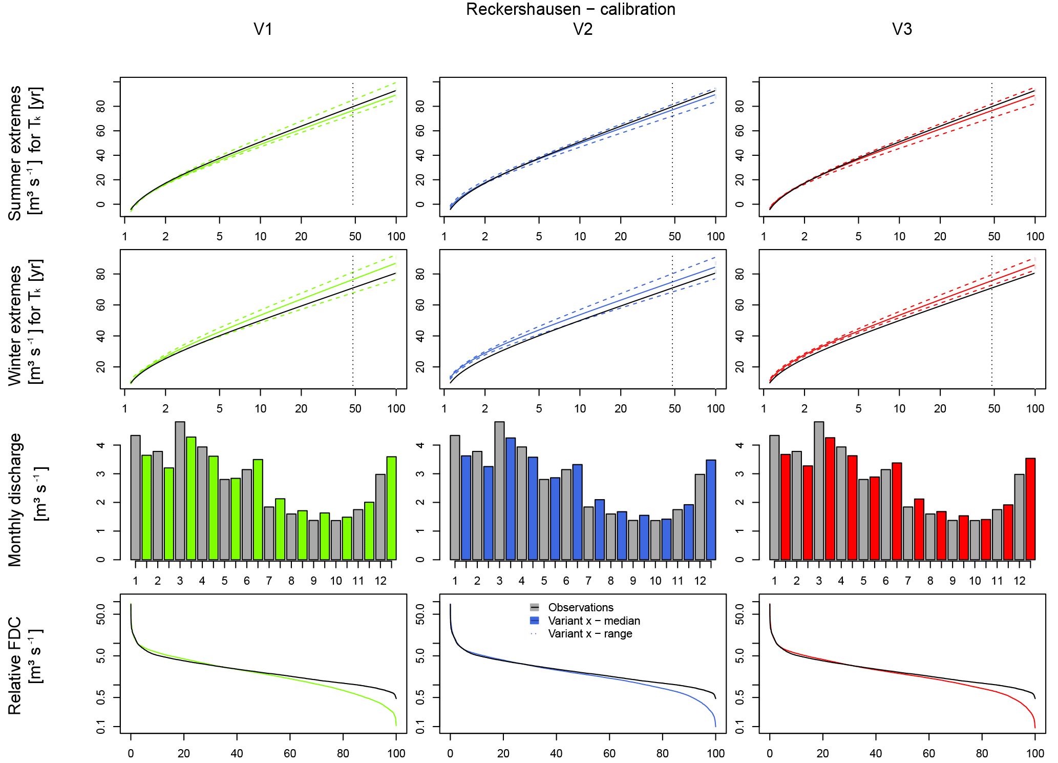
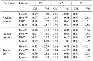
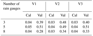
The parameterization was carried out by a split sampling technique with a calibration and validation period for each catchment. The results for Reckershausen, Pionierbrücke and Tetendorf are shown in Figs. 6, 8 and 9 for the calibration period. For Reckershausen, only results using three rain gauges as input are shown here. For Extr-Su and Extr-Wi, flood quantiles are shown for a return period of 100 years. However, the extrapolation is limited by the length of the simulated runoff time series. As per Maniak (2005), a maximum return period of 3 times the runoff time series length should be used to avoid statistical uncertainties that are too high, caused by extrapolation. This results in 75 years for Pionierbrücke, 21 years for Tetendorf and 45 years for Reckershausen. The discussion of the results is limited to these and more frequent return periods. For a quantitative analysis, NSE values for all criteria and for each catchment are given in Table 6. As mentioned before, NSE values are based on a few supporting points (see Eq. 5). Also, theoretical Gumbel distribution functions with two parameters are compared, which can be similar although the population of each distribution function used is different. Hence, values of 0.99 or even 1.00 can be achieved. On the other hand, small deviations from the observations can lead to even negative NSE values (see, e.g., the discussion of the simulation results for Reckershausen).
Table 6NSE values for all catchments and all criteria for calibration (Cal) and validation (Val) periods.

For Reckershausen, the Extr-Su and Extr-Wi are similar to those from observations (Fig. 6). While for summer all observed flood quantiles are within the range of Extr-Su (), for Extr-Wi a slight overestimation occurs for V2 and V3.
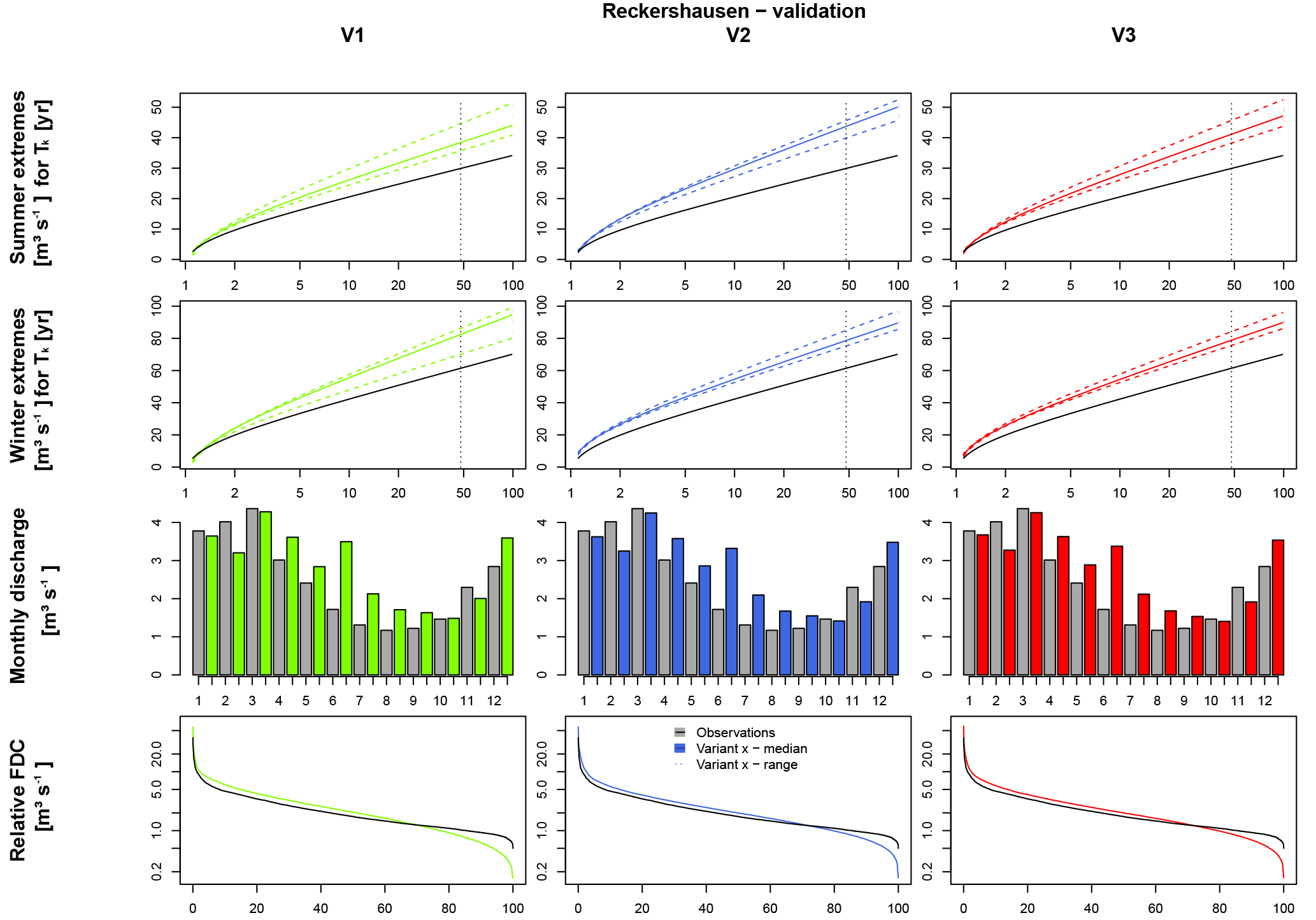
For the validation period, flood quantiles for both Extr-Su and Extr-Wi are overestimated. The overestimation is higher in winter (approx. 20 m3 s−1 for HQ50) than in summer (approx. 10 m3 s−1). One possible cause can be the higher yearly maximums in the calibration period. It is assumed that parameters, calibrated to achieve high floods, tend to generate larger discharges even if lower yearly maxima are observed. This is also indicated by the results for FDC and Q-mon. Although both are represented well in the calibration period (, ), both criteria are overestimated in the validation period (, ). In the validation period the range, and hence the uncertainty, for both Extr-Su and Extr-Wi, is smaller for V2 and V3 in comparison to V1.
The simulation results of Extr-Su of the validation period for the Reckershausen catchment show the sensitivity of the NSE as a goodness-of-fit criterion. V1 and V3 lead to positive NSE values (0.60 and 0.31), while V2 leads to a negative value of NSE . However, from a visual inspection (see Fig. 7), differences between all three approaches are small and less intense as one might expect from the NSE value itself. The high sensitivity of the NSE makes a direct interpretation of its values more difficult (Schaefli and Gupta, 2007; Criss and Winston, 2008). However, for the calibration process, a high sensitivity leads to an improvement of the simulation results.
Values for the objective function are given in Table 7. For Reckershausen, the objective function values are very similar for V1, V2 and V3 for both calibration and validation periods, especially by taking into account that the value for the objective function depends on four NSE values.
For Pionierbrücke it should be mentioned that at points during the calibration (see the FDC in Fig. 8) and validation periods, a simulated discharge of Q=0 m3 s−1 was obtained. Zero discharge implies that all storages have been emptied. This only occurs for Pionierbrücke and is due to the very steep conditions in the mountainous catchment (see Fig. 1) and hence the low soil depth and storage capacity. In the observed time series the minimum value is Q=0.1 m3 s−1. The underestimation is caused by the selection of criteria selected for the objective function used for calibration as well. The main aim is to represent the extreme flows, while the shapes of the intra-annual cycle of monthly average discharges and of the FDC are only implemented to achieve an overall realistic mean discharge behavior. For the FDC, four quantiles greater than 0.5 and only two quantiles smaller than 0.5 are used. Smaller quantiles are not of interest in these simulations, since discharge values in that range belong to dry periods with low flows, for which daily values of rainfall are sufficient for simulations and hence no rainfall disaggregation would be necessary. For the FDC, V3 leads to a slightly better fit to observations for non-exceedance probabilities smaller than 35 %, but to a worse fit between 35 % and 60 % non-exceedance probability. However, FDC is underestimated, independent of the applied rainfall product, for non-exceedance probabilities higher than 60 %. The underestimation identified by the FDC can also be identified for Q-mon in winter and in the underestimation of the Extr-Su and Extr-Wi. The results for the validation period are very similar and not shown here.
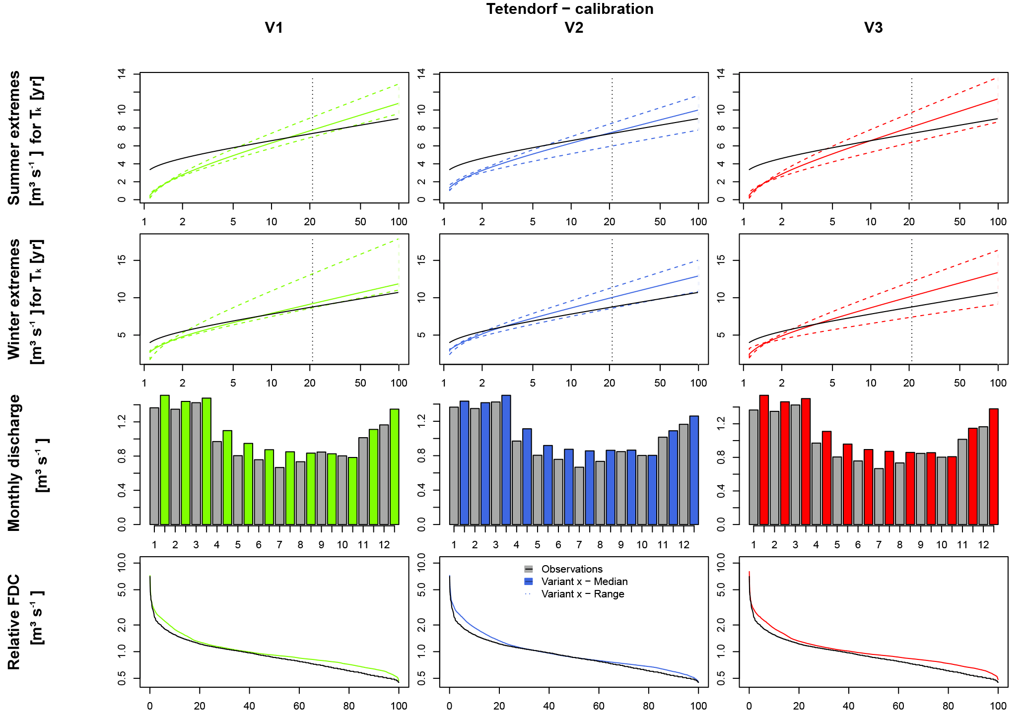
In contrast, for Tetendorf, FDC and Q-mon (except September and October) are overestimated by all rainfall products (Fig. 9). However, for Q-mon the shape of the intra-annual cycle is represented well. For the extreme values it should be mentioned again that the analyses are only valid for return periods more frequent than 21 years. For Extr-Su, underestimations occur for return periods more frequent than 5 years for all variants in the calibration period (less than 2 years in the validation period). For Extr-Wi, the median of V1 represents the observed values well, while for V2 and V3 the median leads to overestimations for return periods frequent than 5 years. However, observations are still in the range of the simulation results, whereby the range is wider for V1 and V3 in comparison to V2. In total, the resampling in V2 leads to a reduction of the overestimation of the observed summer extreme values, but to a stronger overestimation for winter extremes in comparison to V1 and V3.
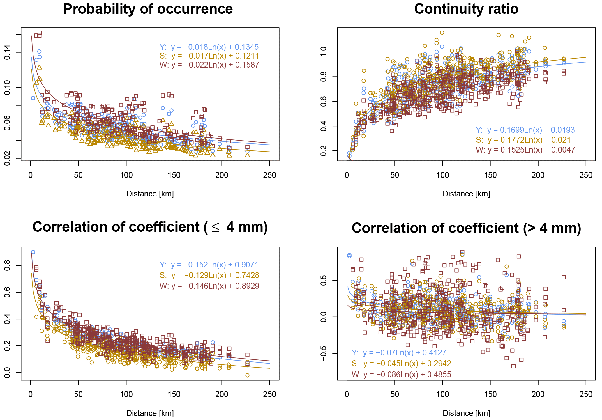
Figure 10Bivariate spatial characteristics estimated for summer (S) and winter (W) seasons as well as over the whole year (Y).
Since for Tetendorf seasonal differences regarding V2 were identified, the spatial rainfall characteristics of the objective function applied for the resampling process have been re-analyzed, differing between the summer and winter half years. The results regarding both periods as well as the estimation over the complete year are shown in Fig. 10 for all bivariate spatial rainfall characteristics based on all 24 hourly stations in Lower Saxony that have been used before for the estimation of these characteristics (Müller, 2016). For the continuity ratio, probability of occurrence and both volume classes of correlation coefficients, differences can be identified, based on the different geneses of rainfall in summer and winter. The probability of rainfall occurrence is lower in summer due to a higher number of convective rainfall events. However, the distance-dependent curve progression is very similar between the seasonal and annual estimated spatial characteristics. Since spatial characteristics are just moved closer to the regression line by V2 (without a perfect fit; see Fig. 4), an improvement of the spatial rainfall characteristics by introducing slightly different season-dependent regression lines cannot be expected and is hence not applied.
As main reasons for the seasonal differences, the short validation and calibration periods are considered. Short periods mean a small number of days with rain and hence a small number of relative diurnal cycles to swap during the resampling, limiting the ability of the algorithm to improve the spatial characteristics. The usage of time series of V2 as input for HBV and the additional short time for the calibration process lead to the seasonal differences.
For longer calibration and validation periods (Reckershausen and Pionierbrücke) the results for V1, V2 and V3 are very similar regarding the runoff statistics. An influence of the chosen method on the implementation of spatial consistence cannot be recognized.
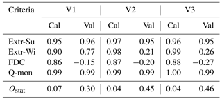
Table 7Ostat values for all catchments and all criteria for calibration (Cal) and validation (Val) periods.
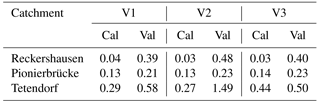
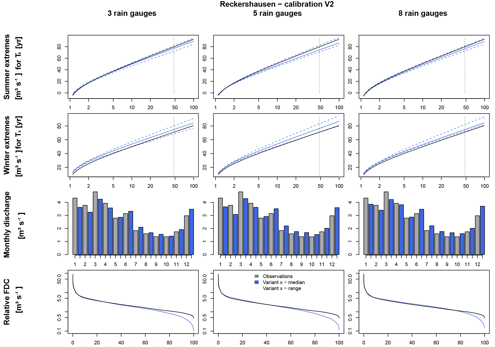
Figure 11Runoff simulation results for V2 with three, five and eight rain gauges with HBV for Reckershausen, calibration period.
(b) HBV simulation results' calibration using different numbers of rain gauges as input
A possible reason for the non-visible influence of the chosen method for the implementation of spatial consistence in the simulated runoff statistics is the low rain gauge network density. With a low network density, it is not possible to reflect the spatial rainfall variability, and hence the influence of V1, V2 and V3 cannot be identified. The influence of the spatial rainfall variability on the runoff can only be determined by rainfall–runoff simulations.
Therefore, for Reckershausen, different numbers of rain gauges are applied for the calculation of the areal rainfall used as input for HBV. Areal rainfall is estimated by three rain gauges (representing a network density of 0.9 gauges per 100 km2) as carried out in (a), five rain gauges (1.6 gauges per 100 km2) and eight rain gauges (2.5 gauges per 100 km2). The results are shown for V2 in Fig. 11 for the calibration and in Fig. 13 for the validation period. The results for V1 and V3 are very similar and not shown here. However, for a quantitative analysis the NSE and Ostat values are shown in Tables 8 and 9.

Figure 12Runoff simulation results for V2 with three, five and eight rain gauges with HBV for Reckershausen, validation period.
Again, independent of the number of rain gauges used for the estimation of the areal rainfall, the results from the calibration period (Fig. 11) represent the observations better than those from the validation period (Fig. 12). In the validation period, Extr-Su and Extr-Wi are overestimated as well as the majority of Q-mon and the FDC. Minor differences can be identified between the different rain gauge network densities, but no general conclusion is possible; e.g., the overestimation of Extr-Wi in the calibration period is increasing with an increasing network density. However, in the validation period, the overestimation is decreasing with an increasing number of rain gauges from three to eight. Also for Q-mon or the FDC, no systematic improvement can be identified. This is an unexpected finding because with the additional information from the daily total rainfall amounts, an improvement of at least the continuum characteristics was expected. Also for the NSE and Ostat values, no systematical improvement can be identified: Ostat(V2, three rain gauges) = 0.03, Ostat(V2, five rain gauges) = 0.04 and Ostat(V2, eight rain gauges) = 0.03 (see Tables 8 and 9).
Table 8NSE values for all catchments and all criteria for calibration (Cal) and validation (Val) periods.
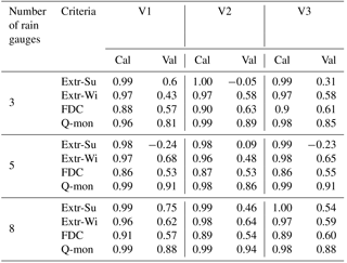
Table 9Ostat values for all catchments and all criteria for calibration (Cal) and validation (Val) periods.
It can be summarized that the number of rain gauges has only a minor but no systematic influence on runoff statistics for the catchments used in this study. This contradicts conclusions from other studies. Seliga et al. (1992) recommend information every 5 km2 (20 rain gauges per 100 km2) for spatial rainfall applications. So an improvement by an increasing station density up to this threshold should have been expected. For a French catchment with an area size of 71 km2, Obled et al. (1994) investigated the influence of using 5 or 21 rain gauges, representing rain gauge network densities of 7 and 22 rain gauges per 100 km2. With 21 rain gauges Obled et al. (1994) improved their results significantly. Nevertheless, they conclude that the improvement is based on the better estimation of the total rainfall amount, not on its spatial distribution. Xu et al. (2013) investigated the influence of station density on a Chinese catchment with an area size of 94 660 km2 and daily rainfall time series; hence a direct comparison of network densities is not possible. Nevertheless, they point out that the distribution of rain gauges inside the catchment is of importance. A distribution covering regions with different rainfall behaviors in a catchment can lead to better simulation results with only a few rain gauges in comparison to a less efficiently distributed network with more rain gauges. In the current study, the rain gauges for each network density scenario have been selected in a way that covers the catchment area and its rainfall representatively (see Fig. 2). This could be one reason why an increase in rain gauge network density shows no systematic improvement in this study.

Figure 13Runoff simulation results with HBV without calibration for Reckershausen, validation period.
(c1) HBV simulation results without calibration using three rain gauges as input
Another possible reason for the small differences between V1, V2 and V3 is the calibration of the rainfall–runoff model parameters for each of the rainfall products. Parameters are allowed to vary between V1, V2 and V3, and hence damp the effects of the different degrees of spatial consistence. To exclude the calibration as a possible reason for the damping behavior, a calibration with a neutral rainfall product offering the same spatial rainfall coverage without giving preference to one of the investigated versions would be recommended. This would enable a direct comparison between V1, V2 and V3 without re-calibration of the models. Since high-resolution time series do not exist with the required spatial network density, radar data could be a possible solution. However, radar time series are too short for model simulations and subsequent derived flood frequency analyses.
To avoid recalibrations, a pragmatic solution is chosen: for each parameter, the arithmetic mean of the upper and lower bound for each parameter (as described by Wallner et al. (2013); see also Table S2) is utilized to form what is called a “default” parameter set. The default parameter set is independent of calibration and therefore observed rainfall data, which in turn might have stronger similarities to a certain rainfall product, and hence might introduce biases in the comparison of rainfall products. In this way, we do not attempt to provide highest accuracy through utilizing the default parameter set. Instead, we intend to provide reliable first guesses that do not favor V1, V2 or V3. The application of a default parameter set includes some shortcomings, e.g., regarding the physical interpretability, but it enables a comparison of the rainfall products.
For the validation period, simulation results based on this default parameter set have been analyzed. Although a splitting in calibration and validation period is not necessary if no calibration is carried out, comparisons are possible between the simulation results with and without calibrated parameters. The results are shown in Fig. 13 for Reckershausen; results are similar for Pionerbrücke and Tetendorf. For a quantitative evaluation, NSE values for all catchments are provided in Table S6 and Ostat values in Table S7.
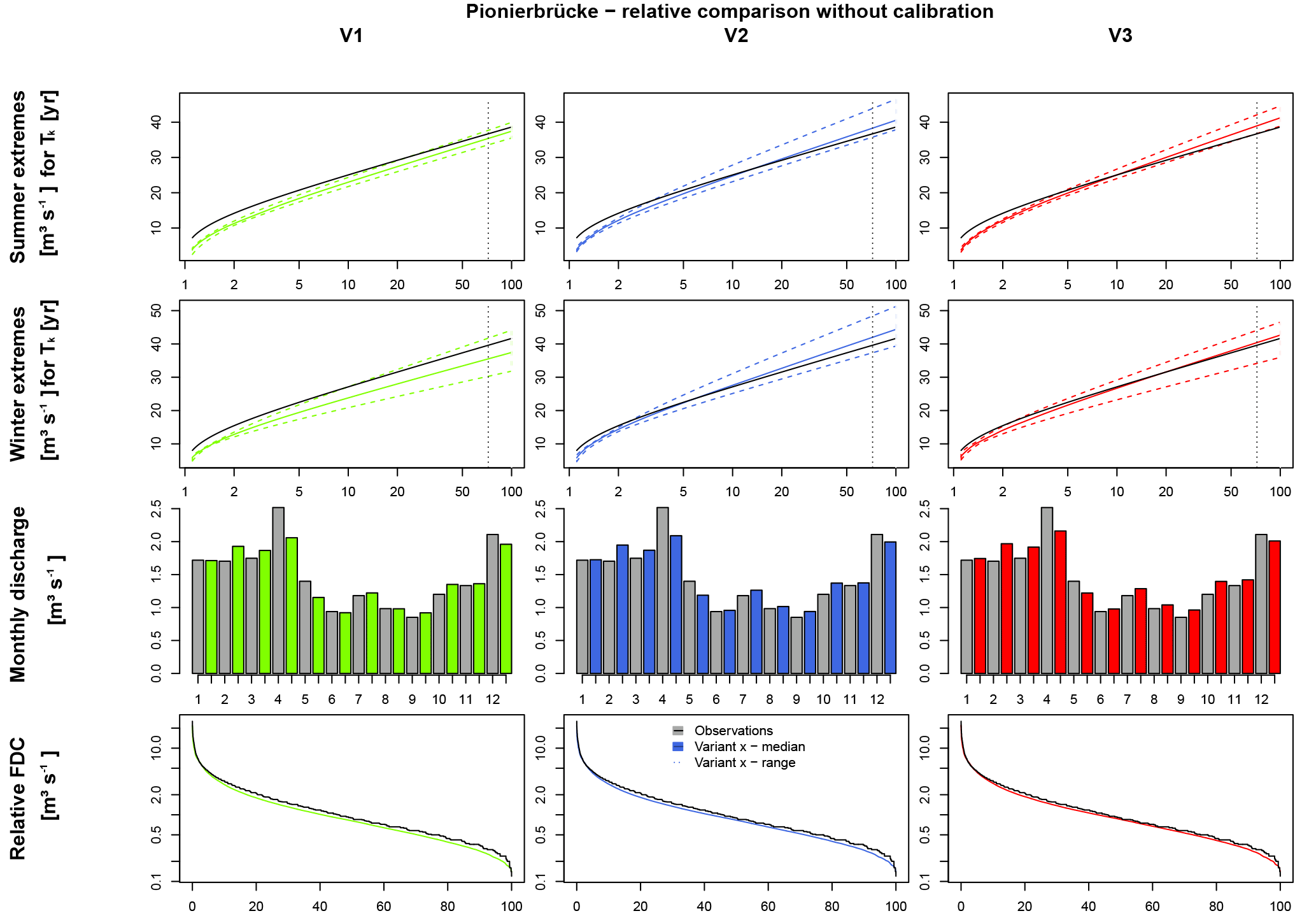
Figure 14Runoff simulation results with WaSiM without calibration for Pionierbrücke, calibration period.
For Pionierbrücke and Tetendorf simulation results are worse without calibration (e.g., for Pionierbrücke, V1: and ). For Reckershausen a slight improvement can be identified without calibration. In the validation period, the calibrated parameters led to an overestimation of extreme values for both seasons as well as an overestimation of FDC and Q-mon (e.g., for V3: and ). For all catchments, Extr-Su is underestimated by every version of spatial consistence. Extr-Wi is also underestimated for Reckershausen and Pionierbrücke, but overestimated for Tetendorf. For all catchments, an intra-annual cycle of Q-mon can be identified. For Reckershausen, Q-mon is similar to observations, while for Pionierbrücke underestimations can be identified and for Tetendorf overestimations can be identified in winter. The FDC is not represented well for any of the catchments. However, the results based on the default parameter sets provide feasible estimates of the hydrological response of the catchments without calibration. In this way, the default parameter set provides a possible way to compare different rainfall products without favoring one of them. As the model parameters are not representing the real behavior of the catchments, this procedure is a pure relative comparison between the rainfall products (V1, V2, V3) and not valid for a comparison between the simulation results and observed data.
Although a default set of parameters has been applied, the differences in the simulation results between V1, V2 and V3 are still small. For Pionierbrücke, the values of the objective function show the same range without and with calibration (1.10 (V2) (V1) or 0.21 (V1) (V2, V3)). The similarity of the simulation results exists even if the model parameters are not calibrated and a default parameter set is used.
(c2) WaSiM simulation results without calibration using three rain gauges as input
For the comparison of V1, V2 and V3, WaSiM (Schulla, 1997, 2015) is used as an additional rainfall–runoff model. The application of more than one model increases the reliability of the simulation results and excludes the possibility of being model-dependent. As far as possible, the same parameter values as in HBV in the uncalibrated case (c1) have been applied. The investigation with WaSiM is carried out only for the Pionierbrücke catchment, since here the highest differences in simulation results are expected due to the short reaction time of the catchment.

Figure 15Runoff simulation results with WaSiM without calibration for Pionierbrücke, validation period.
The results are shown in Fig. 14 for the calibration period and Fig. 15 for the validation period, and a quantitative analysis is given in Table 10. For the calibration and the validation period, Extr-Su and Extr-Wi are simulated slightly higher with V2 and V3 in comparison to V1. In addition, the range for both criteria is higher for V2 and V3 in comparison to V1, whereby V2 leads to even wider ranges than V3 in some cases (e.g., Extr-Win the validation period). This is consistent with the areal rainfall extremes presented for Pionierbrücke in Fig. 5. In this context it should be repeated that a relative comparison is carried out and under- or overestimations are not points of interest. The NSE values for both Extr-Su and Extr-Wi are very similar for V2 and V3 (e.g., NSE and NSE), but show differences to V1 (NSE). Hence, in WaSiM a slight effect of the spatial consistence of rainfall is visible from the simulation results. Possible reasons for the differences are the spatial resolution (150 m×150 m for each raster cell). However, for FDC and Qmon, values for V1, V2 and V3 are again very similar. While for the calibration period the Ostat values are similar for all rainfall products, in the validation period the Ostat values for V2 and V3 ( and ) are much closer to each other than to V1 ().
Table 10NSE and Ostat values for Pionierbrücke without parameter calibration using WaSiM.
The rainfall–runoff simulation results with HBV after calibration of the parameters show that with all three rainfall products, V1, V2 and V3, the Extr-Su and Extr-Wi, the FDC and Q-mon can be represented with a comparable quality. Although the focus is on the representation of the seasonal extreme values of runoff, Extr-Su and Extr-Wi, cumulative runoff statistics (Q-mon, FDC) are additionally applied to also capture the general behavior of the catchments. The differences between the three methods are very small for the majority of all cases. Possible reasons for these small differences, which are discussed below, are as follows:
- -
small differences between the three rainfall products,
- -
dampening of those differences by the calibration of the rainfall–runoff model parameters,
- -
dampening behavior of the catchments,
- -
choice of the rainfall–runoff model and its ability to represent differences of the three rainfall products.
Small differences between V1, V2 and V3 would lead to small differences in rainfall–runoff simulation results. However, the differences between the three methods are apparent. For the bivariate spatial characteristics (Fig. 4), the areal rainfall intensities (see Fig. S5) and the areal rainfall extremes (Fig. 5), differences can be identified among all three methods, which should be reflected by the runoff statistics results as well.
Another cause can be the separate calibration of the rainfall–runoff model parameters for each method. The calibration strategy applied has the capability to harmonize the different rainfall products with the runoff statistics used for calibration. For the discussion of this harmonization effect, the simulation results for Reckershausen during the calibration (Fig. 11) and validation periods (Fig. 12) are used. During the calibration period, higher values for Extr-Su and Extr-Wi can be found in the observed runoff data. Hence, the parameters calibrated in this period tend to lead to higher runoff values. This is proven by the simulation results of the validation period with an overestimation of all runoff statistics. Only through the usage of an uncalibrated parameter set can the calibration be excluded from the list of possible causes.
The dampening behavior of the investigated catchments depends on the size and the concentration time of a catchment (Andrés-Doménech et al., 2015). Also, catchments act as a filter, so rainfall as an input signal is dampened during its transformation to runoff by several processes (e.g., interception, losses due to storage filling, transport processes). Mandapaka et al. (2009) have analyzed the runoff response from different rainfall scenarios with a total amount of 10 mm for (sub)catchments of different sizes. For catchments with an area less than 10 km2, a strong dependence of the duration, the intensity and the spatial distribution of the rainfall is identified. With increasing area size, the influence of these factors is reduced, and for catchments with 1000 km2, it is almost completely dampened. Since the catchment areas in the current study range between 44 and 321 km2, i.e., considerably larger than 10 km2, this could be a possible reason why the differences in the runoff results are so small. On the other hand, the results of Seliga et al. (1992) and Obled et al. (1994) show that an increasing station network density leads to an improvement of rainfall information and hence should also lead to an improvement of the runoff simulation results. Ogden and Julien (1993) investigate the time of concentration of a catchment as an influencing factor in rainfall–runoff processes. If the duration of a rainfall event causing flooding is shorter than the time of concentration, the spatial distribution of the rainfall is influencing the discharge at the catchment outlet. If rainfall events last longer than the concentration time, the influence decreases. However, Nicotina et al. (2008) only identify an influence of spatial rainfall patterns for catchments with areas >1000 km2, based on the travel time in the catchment. In the investigated catchments, the concentration time ranges from 1.8 to 7.4 h, so the temporal and spatial variation should have an influence on the simulated discharges. In Müller and Haberlandt (2018) the rainfall products V1 and V2 and their influence on simulated discharge have been analyzed for 5 min time steps in an urban hydrological context. Significant differences could be identified between the simulated runoff statistics resulting from V1 and V2 for their artificial sewage system.
Another reason could be the choice of the rainfall–runoff model. Obled et al. (1994) raise the question whether it is possible with semi-distributed models to transfer the information of the spatial rainfall patterns into the simulated discharge time series. Obversely, if spatial rainfall patterns are necessary for rainfall–runoff simulations for a catchment with an area size of 71 km2, as is used in their study, the spatial resolution of semi-distributed models may not be sufficient. Krajewski et al. (1991) also conclude that for the analysis of spatial problems, fully distributed models may be more suitable and recommend those for further studies. Bárdossy and Das (2008) point out that with an increasing spatial resolution of the applied rainfall–runoff model, the sensitivity of, for example, the rain gauge density, and hence the spatial rainfall patterns, may increase as well. The rainfall–runoff simulations were carried out with two models, the semi-distributed HBV model and the fully distributed WaSiM model. The spatial resolution is much higher in WaSiM with 150 m×150 m for each raster cell than in HBV with approx. 20 km2 per subcatchment. This higher spatial rainfall diversity and hence a numerical diffusion of the rainfall due to too coarse spatial resolution is thus avoided. Through the rainfall correction for altitude, an additional increase of the spatial diversity is achieved. While for the simulated discharge time series with HBV, almost no differences between the different rainfall products could be identified, for the Pionierbrücke catchment in WaSiM, slight differences between method V1 and methods V2 and V3 regarding the seasonal extreme values can be identified. For both V2 and V3, subsequent steps after the rainfall disaggregation were applied to implement spatial consistence by simultaneous rainfall occurrence at different rain gauges. This affects the simulated runoff at least for instantaneous peak flows in the summer and winter period. However, the number of subcatchments in HBV and therefore the spatial resolution of the rainfall–runoff model can be increased, which is assumed to lead to more diverse results between V1, V2 and V3, similar to results from WaSiM.
For Pionierbrücke, as a fast-reacting, mountainous catchment, the absolute differences for the seasonal extreme flows resulting from V1 or the products V2 and V3 for a flood with a return period of 50 years are approx. 5–8 m3 s−1 during both the calibration and validation periods (see Figs. 14 and 15) using WaSiM. For the other two catchments, Reckershausen and Tetendorf, the difference is expected to be smaller since both catchments are larger and cover an area that is less steep. Thus, no additional simulations with WaSiM have been carried out for these two catchments. In this context it should be mentioned that WaSiM is a much more complex rainfall–runoff model than HBV with a high demand on meteorological input time series (e.g., precipitation, temperature, humidity, wind speed and global radiation), which have to be available for the whole simulation period on an hourly time step.
The aim of this study is to explore the influence of different degrees of spatial consistence in disaggregated time series on simulated runoff statistics. The study is carried out for three mesoscale catchments in Lower Saxony, Germany, which differ in terms of their size, land use, soil and slope. For the disaggregation, a multiplicative, microcanonical cascade model according to Müller and Haberlandt (2015) is used. Since the disaggregation process is performed on a station by station basis without taking neighboring stations into account, spatial consistence must be implemented afterwards. Here, a resampling algorithm based on Müller and Haberlandt (2015) is applied (named V2) as well as a more pragmatic approach, whereby the same relative diurnal cycle is used for all stations on the one day (Haberlandt and Radtke, 2014; named V3). Nevertheless, investigations without subsequent steps to implement spatial consistence exist as well (Ding et al., 2016) and have been included in this study (named V1). The hypothesis tested in this study is that these different rainfall products lead to differences in the derived runoff statistics as well. The following conclusions can be drawn regarding the rainfall product differences:
- 1.
The resampling algorithm for the implementation of spatial consistence was applied on an hourly basis for the first time for distances smaller than 20 km for V2. The achieved values for the bivariate spatial rainfall characteristics are comparable to those from observations.
- 2.
The bivariate spatial characteristics are underestimated by V1 and overestimated by V3 respectively.
- 3.
While for the areal rainfall intensities, the exceedance curve leads to an expected order of V1 < V2 < V3, for the areal rainfall extremes, V2 and V3 result in similar values, both being higher than V1.
The generated rainfall products V1, V2 and V3 have been used as input for rainfall–runoff modeling to evaluate the influence of the differences of rainfall characteristics identified above. An application-based evaluation is important in terms of rainfall generation, since it provides a new perspective and hence new insights into the rainfall data (Müller and Haberlandt, 2018; Müller et al., 2017; Sikorska et al., 2018). For the simulations, the semi-distributed HBV model (Wallner et al., 2013) and the fully distributed WaSiM model (Schulla, 1997, 2015) have been implemented. The essential findings are as follows:
- 1.
With the applied calibration process in HBV, a good representation of observed runoff statistics is possible for V1–V3 for the calibration period.
- 2.
The rainfall products V1–V3 result in only small differences in the simulated runoff statistics using HBV. Differences do not increase whether a default parameter set without calibration is applied or if the station density increases.
- 3.
For peak flows in the summer and winter periods, slight differences resulting from V1 and both V2 and V3 can be identified using WaSiM. V2 and V3 lead to comparable higher flood peaks than V1, which is consistent with extreme value analysis of areal rainfall for this catchment.
- 4.
For the intra-annual cycle and the flow duration curve, no difference resulting from V1–V3 can be identified from either HBV or WaSiM.
By the application of V1 as input rainfall data and HBV as a rainfall–runoff model, Ding et al. (2016) achieved a good representation of summer and winter peak flows. Haberlandt and Radtke (2014) applied HEC-HMS (Feldman, 2000) as a semi-distributed rainfall–runoff model with disaggregated and parallelized rainfall time series (V3) as input data. The continuously simulated runoff time series were analyzed regarding annual extreme flows, which could be reproduced well for all catchments. The findings of both investigations can be confirmed by the current study.
However, no differences resulting from V1, V2 and V3 regarding the summer and winter extremes are detectable for HBV.
On the other hand, WaSiM results in slight differences for seasonal extreme values for Pionierbrücke, the investigated catchment, which is in line with previous findings regarding the areal rainfall extreme values. However, the differences between the resulting seasonal peak flows simulated with WaSiM from V1, V2 and V3 are still small with approx. 5–8 m3 s−1 (up to 15 %) for floods with return periods of 50 years. It should be noted that V1, V2 and V3 clearly differ regarding the investigated spatial bivariate characteristics of probability of occurrence, coefficient of correlation, continuity ratio and the resulting areal rainfall intensities, especially regarding their extreme values. Hence, the hypothesis formulated before is rejected in this case study. Although several possible causes regarding the applied rainfall–runoff models (parameter calibration, rainfall station density, type and spatial resolution of rainfall–runoff model) have been analyzed, no final conclusion about the reason for the similar runoff statistic can be drawn. It is assumed that the damping behavior of the catchments leads to these small differences in runoff statistics.
These findings suggest that (i) simple model structures might compensate for deficiencies in spatial representativeness through parameterization and (ii) highly resolved hydrological models benefit from improved spatial modeling of rainfall.
Of course, the similarity of the simulated runoff statistics from V1, V2 and V3 is only valid for the investigated catchments. For catchments with other climatic or physiographic attributes, results can be different. Therefore, a systematic investigation of catchments with different hydrological behavior in climates and with different rainfall–runoff models would be necessary (comparative hydrology) to identify catchments for which the degree of spatial rainfall consistence matters. The current study could be a starting point for this.
However, the main intention of the current study was to analyze the impact of rainfall products with different degrees of spatial consistence on simulated runoff statistics. The application of the resampling algorithm (V2) is recommended for the spatial application of disaggregated rainfall data since this method leads to the best agreement with the observed spatial rainfall characteristics.
The disaggregated and modified time series as well as all simulation results are available from the leading author on request. For the rainfall observations please contact the German Weather Service. For the discharge observations several sources have been used: please contact the leading author for details.
The supplement related to this article is available online at: https://doi.org/10.5194/hess-22-5259-2018-supplement.
The authors declare that they have no conflict of interest.
First of all, the two reviewers Anna Sikorska and Nadav Peleg and the editor
Florian Pappenberger are gratefully acknowledged. Their suggestions and
comments helped to improve the manuscript significantly. The authors also
thank former student Jennifer Ullrich for calibration of the simulated
annealing parameters. Thanks are also given to Ross Pidoto for useful
comments on an earlier draft of the manuscript. Special thanks are given to
Bastian Heinrich for technical support during the study. We are also thankful
for the permission to use the data of the German National Weather Service.
Funding was provided for Hannes Müller-Thomy as a Research Fellowship (MU
4257/1-1) by DFG e.V., Bonn, Germany.
The publication of this article was funded by the open-access
fund of Leibniz Universität Hannover.
Edited by: Florian Pappenberger
Reviewed by: Anna Sikorska and Nadav Peleg
Aarts, E. and Korst, J.: Simulated Annealing and Boltzmann Machines: A stochastic approach to combinatorial optimization and neural computing, John Wiley & Sons, Chichester, UK, 1965.
Andrés-Doménech, I., García-Bartual, R., Montanari, A., and Marco, J. B.: Climate and hydrological variability: the catchment filtering role, Hydrol. Earth Syst. Sci., 19, 379–387, https://doi.org/10.5194/hess-19-379-2015, 2015.
Bárdossy, A. and Das, T.: Influence of rainfall observation network on model calibration and application, Hydrol. Earth Syst. Sci., 12, 77–89, https://doi.org/10.5194/hess-12-77-2008, 2008.
Bergström, S.: Development and application of a conceptual runoff model for Scandinavian catchments, SMHI Report RHO 7, Norrköping, 134 pp., 1976.
Beven, K. J.: Rainfall-Runoff Modelling: The Primer, John Wiley and Sons, Chichester, UK, 2001.
Bormann, H. and Elfert, S.: Application of WaSiM-ETH model to Northern German lowland catchments: model performance in relation to catchment characteristics and sensitivity to land use change, Adv. Geosci., 27, 1–10, https://doi.org/10.5194/adgeo-27-1-2010, 2010.
Breinl, K., Turkington, T., and Stowasser, M.: Simulating daily precipitation and temperature: A weather generation framework for assessing hydrometeorological hazards, Meteorol. Appl., 22, 334–347, 2014.
Criss, R. E. and Winston, W. E.: Do Nash values have value? Discussion and alternate proposals, Hydrol. Process., 22, 2723–2725, 2008.
Ding, J., Wallner, M., Müller, H., and Haberlandt, U.: Estimation of instantaneous peak flows from maximum mean daily flows using the HBV hydrological model, Hydrol. Process., 30, 1431–1448, 2016.
DVWK: Ermittlung der Verdunstung von Land- und Wasserflächen, in: DVWK-Merkblatt 238/1996, edited by: ATVDVWK-Regelwerk, Deutscher Verband für Wasserwirtschaft und Kulturbau e.V. (DVWK), Bonn, Germany, 1996.
DVWK: Verdunstung in Bezug zu Landnutzung, Bewuchs und Boden, Merkblatt ATV-DVWK-M 504, Deutsche Vereinigung für Wasserwirtschaft, Abwasser und Abfall, Hennel, 2002.
Fangmann, A. and Haberlandt, U.: Statistical approaches for assessment of climate change impacts on low flows: temporal aspects, Hydrol. Earth Syst. Sci. Discuss., https://doi.org/10.5194/hess-2018-284, in review, 2018.
Federal Environment Agency: CORINE Land Cover, DLR-DFD, Hannover, 1996, 2009.
Feldman, A. D.: Hydrological Modeling System HEC-HMS – Technical Reference Manual, 145 pp., US Army Corps of Engineers, Davis, 2000.
Förster, K., Hanzer, F., Winter, B., Marke, T., and Strasser, U.: An open-source MEteoroLOgical observation time series DISaggregation Tool (MELODIST v0.1.1), Geosci. Model Dev., 9, 2315–2333, https://doi.org/10.5194/gmd-9-2315-2016, 2016.
Gelleszun, M., Kreye, P., and Meon, G.: Representative parameter estimation for hydrological models using a lexicographic calibration strategy, J. Hydrol., 553, 722–734, https://doi.org/10.1016/j.jhydrol.2017.08.015, 2017.
Gires, A., Giangola-Murzyn, A., Abbes, J.-B., Tchiguirinskaia, I., Schertzer, D., und Lovejoy, S: Impacts of small scale rainfall variability in urban areas: a case study with 1D and 1D/2D hydrological models in a multifractal framework, Urban Water J., 12, 607–617, 2015.
Haberlandt, U., Ebner von Eschenbach, A.-D., and Buchwald, I.: A space-time hybrid hourly rainfall model for derived flood frequency analysis, Hydrol. Earth Syst. Sci., 12, 1353–1367, https://doi.org/10.5194/hess-12-1353-2008, 2008.
Haberlandt, U. and Radtke, I.: Hydrological model calibration for derived flood frequency analysis using stochastic rainfall and probability distributions of peak flows, Hydrol. Earth Syst. Sci., 18, 353–365, https://doi.org/10.5194/hess-18-353-2014, 2014.
Hartwich, R., Behrens, J., Eckelmann, W., Haase, G., Richter, A., Roeschmann, G., and Schmidt, R.: Bodenübersichtskarte der Bundesrepublik Deutschland, Bundesanstalt für Geowissenschaften und Rohstoffe, Hannover, Germany, 1998.
Hosking, J. and Wallis, J.: Regional Frequency Analysis: an approach based on L-moments, Cambridge University Press, New York, USA, 1997.
Kirkpatrick, S., Gelatt, C. D., and Vecchi, M. P.: Optimization by simulated annealing, Science, 220, 671–680, 1983.
Kirpich, Z. P.: Time of concentration of small agricultural watersheds, Civil Eng., 10, 1940.
Krajewski, W. F., Lakshmi, V., Georgakakos, K. P., and Jain, S. C.: A Monte Carlo study of rainfall sampling effect on a distributed catchment model, Water Resour. Res., 27, 119–128, 1991.
Mandapaka, P. V., Krajewski, W. F., Mantilla, R., and Gupta, V. K.: Dissecting the effect of rainfall variability on the statistical structure of peak flows, Adv. Water Resour. 32, 1508–1525, 2009.
Mandelbrot, B. B.: Intermittent turbulence in self-similar cascades: divergence of high moments and dimension of the carrier, J. Fluid Mech., 62, 331–358, 1974.
Maniak, U.: Hydrologie und Wasserwirtschaft, Springer Verlag, Berlin, Germany, 2005.
Melsen, L. A., Teuling, A. J., Torfs, P. J. J. F., Uijlenhoet, R., Mizukami, N., and Clark, M. P.: HESS Opinions: The need for process-based evaluation of large-domain hyper-resolution models, Hydrol. Earth Syst. Sci., 20, 1069–1079, https://doi.org/10.5194/hess-20-1069-2016, 2016.
Monteith, J. L.: Evaporation and environment, in the State and Movement of Water in Living Organisms, edited by: Fogg, G. E., Symposia of the Society for Experimental Biology, Cambridge University Press, Cambridge, 19, 205–234, 1965.
Müller, H.: Rainfall disaggregation for hydrological modeling, PhD thesis, Proceedings of the Institute of Water Resources Management, Hydrology and Agricultural Hydraulic Engineering, 101, Hannover, 197 pp., 2016 (in German).
Müller, H. and Haberlandt, U.: Temporal Rainfall Disaggregation with a Cascade Model: From Single-Station Disaggregation to Spatial Rainfall, J. Hydrol. Eng., 20, 04015026, https://doi.org/10.1061/(ASCE)HE.1943-5584.0001195, 2015.
Müller, H. and Haberlandt, U.: Temporal rainfall disaggregation using a multiplicative cascade model for spatial application in urban hydrology, J. Hydrol., 556, 847–864, 2018.
Müller, T., Schütze, M., and Bárdossy, A.: Temporal asymmetry in precipitation time series and its influence on flow simulations in combined sewer systems, Adv. Water Resour., 107, 56–64, 2017.
Nash, J. E. and Sutcliffe, J. V.: River flow forecasting through conceptual models part I – a discussion of principles, J. Hydrol., 10, 282–290, 1970.
Nicotina, L. E., Celegon, E. Alessi, Rinaldo, A., and Marani, M.: On the impact of rainfall patterns on the hydrologic response, Water Resour. Res., 44, W12401, https://doi.org/10.1029/2007WR006654, 2008.
Niehoff, D., Fritsch, U., and Bronstert, A.: Land-use impacts on storm-runoff generation: scenarios of land-use change and simulation of hydrological response in a meso-scale catchment in SW-Germany, J. Hydrol. 267, 80–93, 2002.
Obled, C., Wendling, J., and Beven, K.: The sensitivity of hydrological models to spatial rainfall patterns: an evaluation using observed data, J. Hydrol., 159, 305–333, 1994.
Ochoa-Rodriguez, S., Wang, L.-P., Gires, A., Pina, R. D., Reinoso-Rondinel, R., Bruni, G., Ichiba, A., Gaitan, S., Cristiano, E., van Assel, J., Kroll, S., Murlà-Tuyls, D., Tisserand, B., Schertzer, D., Tchiguirinskaia, I., Onof, C., Willems, P., und ten Veldhuis, M.-C.: Impact of Spatial and Temporal Resolution of Rainfall Inputs on Urban Hydrodynamic Modelling Outputs: A Multi-Catchment Investigation, J. Hydrol., 531, 389–407, 2015.
Ogden, F. L. and Julien, P. Y.: Runoff sensitivity to temporal and spatial rainfall variability at runoff plane and small basin scales, Water Resour. Res., 29, 2589–2597, 1993.
Olsson, J.: Evaluation of a scaling cascade model for temporal rain-fall disaggregation, Hydrol. Earth Syst. Sci., 2, 19–30, https://doi.org/10.5194/hess-2-19-1998, 1998.
Onof, C., Chandler, R. E., und Kakou, A.: Rainfall modelling using Poisson-cluster processes: a review of developments, Stoch. Env. Res. Risk A., 6, 384–411, 2000.
Paschalis, A., Fatichi, S., Molnar, P., Rimkus, S., and Burlando, P.: On the effects of small scale space–time variability of rainfall on basin flood response, J. Hydrol., 514, 313–327, 2014.
Pathiraja, S., Westra, S., and Sharma, A.: Why continuous simulation? The role of antecedent moisture in design flood estimation, Water Resour. Res., 48, W06534, https://doi.org/10.1029/2011WR010997, 2012.
Peel, M. C., Finlayson, B. L., and McMahon, T. A.: Updated world map of the Köppen-Geiger climate classification, Hydrol. Earth Syst. Sci., 11, 1633–1644, https://doi.org/10.5194/hess-11-1633-2007, 2007.
Peleg, N., Blumensaat, F., Molnar, P., Fatichi, S., and Burlando, P.: Partitioning the impacts of spatial and climatological rainfall variability in urban drainage modeling, Hydrol. Earth Syst. Sci., 21, 1559–1572, https://doi.org/10.5194/hess-21-1559-2017, 2017.
Peleg, N., Marra, F., Fatichi, S., Paschalis, A., Molnar, P., and Burlando, P.: Spatial variability of extreme rainfall at radar subpixel scale, J. Hydrol., 556, 922–933, 2018.
Rodriguez-Iturbe, I., Cox, D. R., and Isham, V.: Some models for rainfall based on stochastic point-processes, P. Roy. Soc. A-Math. Phy., 410, 269–288, 1987.
Schaefli, B. and Gupta, H. V.: Do Nash Values have value?, Hydrol. Process., 21, 2075–2080, 2007.
Schulla, J.: Hydrologische Modellierung von Flussgebieten zur Abschätzung der Folgen von Klimaänderungen, Dissertation, ETH Zürich, Switzerland, 1997.
Schulla, J.: Model Description WaSiM (Water balance Simulation Model) – completely revised version of 2012 with 2013 to 2015 extensions, Hydrology Software Consulting J. Schulla, Zürich, Switzerland, 2015.
Seliga, T. A., Aron, G., Aydin, K. and White, E.: Storm runoff simulation using radar-estimated rainfall rates and a Unit Hydrograph model (SYN-HYD) applied to GREVE watershed. American Meteorological Society, 25th International Conference on Radar Hydrology, 587–590, 1992.
Sikorska, A. E., Vivrioli, D., and Seibert, J.: Effective precipitation duration for runoff peaks based on catchment modelling, J. Hydrol., 556, 510–522, 2018.
Sivapalan, M. and Blöschl, G.: Transformation of point to areal rainfall: Intensityduration-frequency curves, J. Hydrol., 204, 150–167, 1998.
Veneziano, D. and Langousis, A.: The areal reduction factor: a multifractal analysis, Water Resour. Res., 41, W07008, https://doi.org/10.1029/2004WR003765, 2005.
Wallner, M. and Haberlandt, U.: Klimabedingte Änderung von Hochwasserabflüssen im Aller-Leine-Einzugsgebiet – Eine Fallstudie mit HBV-IWW, Hydrol. Wasserbewirts., 59, 174–183, 2015.
Wallner, M., Haberlandt, U., and Dietrich, J.: A one-step similarity approach for the regionalization of hydrological model parameters based on Self-Organizing Maps, J. Hydrol., 494, 59–71, 2013.
Westerberg, I. K., Guerrero, J.-L., Younger, P. M., Beven, K. J., Seibert, J., Halldin, S., Freer, J. E., and Xu, C.-Y.: Calibration of hydrological models using flow-duration curves, Hydrol. Earth Syst. Sci., 15, 2205–2227, https://doi.org/10.5194/hess-15-2205-2011, 2011.
Wilks, D. S.: Multisite generalization of a daily stochastic precipitation generation model, J. Hydrol., 210, 178–191, 1998.
Wright, D. B., Smith, J. A., and Baeck, M. L.: A critical examination of area reduction factors, J. Hydrol. Eng., 19, 769–776, 2013.
Xu, H., Chong-Yu, X., Zhang, Z., and Li, L.: Assessing the influence of rain gauge density and distribution on hydrological model performance in a humid region of China, J. Hydrol., 505, 1–12, 2013.
Yu, P. S. and Yang, T. C.: Using synthetic flow duration curves for rainfall–runoff model calibration at ungauged sites, Hydrol. Process., 14, 117–133, 2000.