the Creative Commons Attribution 4.0 License.
the Creative Commons Attribution 4.0 License.
 | 25 Oct 2018
Modelling the water balance of Lake Victoria (East Africa) – Part 2: Future projections
Nicole P. M. van Lipzig
Wim Thiery
Lake Victoria, the second largest freshwater lake in the world, is one of the major sources of the Nile river. The outlet to the Nile is controlled by two hydropower dams of which the allowed discharge is dictated by the Agreed Curve, an equation relating outflow to lake level. Some regional climate models project a decrease in precipitation and an increase in evaporation over Lake Victoria, with potential important implications for its water balance and resulting level. Yet, little is known about the potential consequences of climate change for the water balance of Lake Victoria. In this second part of a two-paper series, we feed a new water balance model for Lake Victoria presented in the first part with climate simulations available through the COordinated Regional Climate Downscaling Experiment (CORDEX) Africa framework. Our results reveal that most regional climate models are not capable of giving a realistic representation of the water balance of Lake Victoria and therefore require bias correction. For two emission scenarios (RCPs 4.5 and 8.5), the decrease in precipitation over the lake and an increase in evaporation are compensated by an increase in basin precipitation leading to more inflow. The future lake level projections show that the dam management scenario and not the emission scenario is the main controlling factor of the future water level evolution. Moreover, inter-model uncertainties are larger than emission scenario uncertainties. The comparison of four idealized future management scenarios pursuing certain policy objectives (electricity generation, navigation reliability and environmental conservation) uncovers that the only sustainable management scenario is mimicking natural lake level fluctuations by regulating outflow according to the Agreed Curve. The associated outflow encompasses, however, ranges from 14 m3 day−1 (−85 %) to 200 m3 day−1 (+100 %) within this ensemble, highlighting that future hydropower generation and downstream water availability may strongly change in the next decades even if dam management adheres to he Agreed Curve. Our results overall underline that managing the dam according to the Agreed Curve is a key prerequisite for sustainable future lake levels, but that under this management scenario, climate change might potentially induce profound changes in lake level and outflow volume.
- Article
(5784 KB) - Companion paper
- BibTeX
- EndNote


Lake Victoria is directly sustaining 30 million people living in its basin and 200 000 fishermen operating from its shores. Therefore, the water level fluctuations of the lake are of major importance. Declining water levels may affect the local communities by their ability to access water, to fish and to transport goods (Semazzi, 2011). Further downstream, the livelihood of about 300 million people in the Nile Basin is supported by the natural resources of Lake Victoria, as it is one of the two major sources of the Nile (Semazzi, 2011). Originating from Lake Victoria, the White Nile provides a more constant flow during the year, providing 70 % to 90 % of the total Nile discharge during the dry season in the Ethiopian highlands, where the second major source is located (Di Baldassarre et al., 2011). A drop in the water level could imply a decreasing outflow, which may have major implications downstream in the Nile Basin. The countries of the Nile Basin require sufficient water resources for their future development and wellbeing, considering the population growth and economic development (Deconinck, 2009; Taye et al., 2011). Consequently, there are a lot of tensions between countries in the Nile Basin. The outflow of the lake is controlled by the Nalubaale and Kiira dams for hydropower generation, located in Jinja (Fig. 1). Human strategies towards regulating the outflow might therefore play a crucial role in the downstream Nile Basin water resources and associated political tensions. This will be even more relevant in the light of climate change, where water will become an even more important resource, both around the lake and downstream in the Nile Basin (Taye et al., 2011). While the released outflow affects the lake level, climate-driven lake level fluctuations also influence the outflow volume released by the dam. The hydropower potential, and thus energy availability in the region, strongly depends on the interplay between outflow and lake levels. Information on the future evolution of the levels and outflow volumes of Lake Victoria is thus vital for future generations living along its shores.
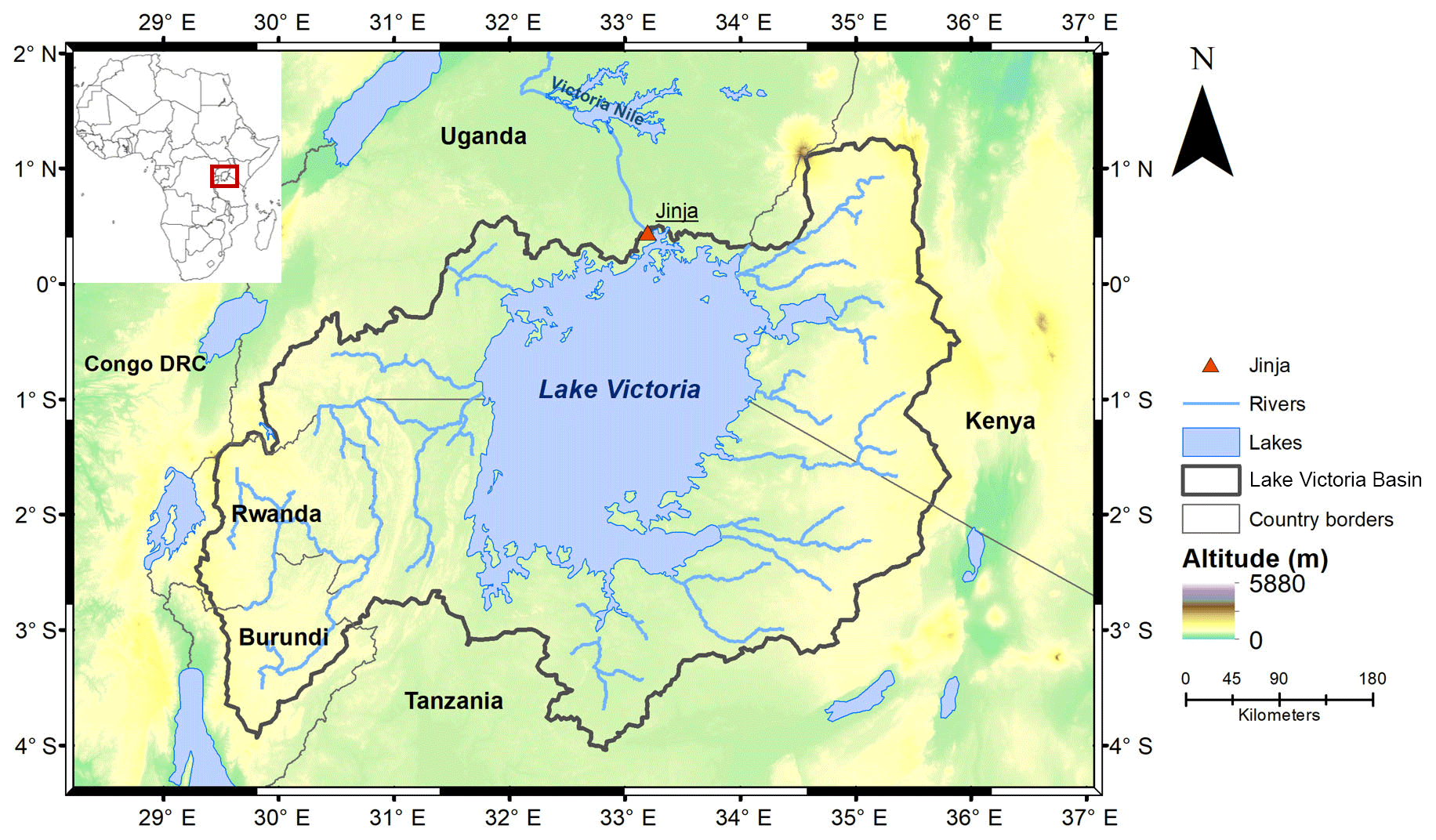
Figure 1Map of Lake Victoria and its basin with surface heights from the Shuttle Radar Topography Mission (SRTM). Taken from Vanderkelen et al. (2018).
The water levels of Lake Victoria are determined by the water balance (WB) of the lake, consisting of precipitation on the lake, lake evaporation, inflow by tributary rivers and dam outflow. Since the construction of the dam complex in 1954, a rating curve called the “Agreed Curve” was established relating the lake level and outflow in natural conditions (Sene, 2000):
In this equation, the dam outflow Qout (m3 day−1) is calculated based on the lake level, L (m), as directly measured at the dam. The Agreed Curve can be used to calculate outflow volumes based on lake levels which lie in the historically observed range going from 10 to 13.5 m measured at the dam (Sutcliffe and Parks, 1999).
The climate in East Africa experiences large interannual variability in precipitation (Nicholson, 2017). The region is a hotspot for climate change, as it is very likely that climate change will have a major influence on precipitation (Kent et al., 2015; Nicholson, 2017; Otieno and Anyah, 2013; Souverijns et al., 2016). Precipitation over the Lake Victoria Basin (LVB) experiences a seasonal cycle with two main rainfall seasons: the long rains in March, April and May and the short rains in September, October and November (Williams et al., 2015). In the last decades, the long rain seasons in East Africa have experienced a series of dry anomalies (Lyon and Dewitt, 2012; Nicholson, 2016, 2017; Rowell et al., 2015; Souverijns et al., 2016; Thiery et al., 2016), while there was no trend observed for the short rains due to a large year-to-year variability (Rowell et al., 2015). This drying trend of the long rains is in contrast with climate model projections for the upcoming decades, projecting an increase in precipitation over East Africa (Kent et al., 2015; Otieno and Anyah, 2013). This apparent contradiction has been called the East African climate paradox of which the causes remain unclear (Rowell et al., 2015). To find explanations, Rowell et al. (2015) stated that more research is needed on the reliability of climate projections over East Africa, for the attribution of changing anthropogenic aerosol emissions and for the role of natural variability in recent droughts. However, Philip et al. (2017) found that the severe drought in northern and central Ethiopia in 2015 is attributable to natural variability and therefore conclude that there is no paradox for this type of event.
Future climate simulations with regional climate models (RCMs) project a decreasing mean precipitation and an increasing evaporation over Lake Victoria (Souverijns et al., 2016; Thiery et al., 2016). Compared to global climate models (GCMs), RCMs have a high spatial resolution and are therefore able to represent regional- and local-scale forcings (Giorgi et al., 2009; Kim et al., 2014). In East Africa, accounting for local variations in topography, vegetation, lakes, soils and coastlines is of major importance, as these variations have a significant effect on the regional climate. Over the LVB, models with sufficiently high resolution are needed to reproduce key circulation features such as the lake–land breeze system (Williams et al., 2015). High-resolution (∼7 km grid spacing) coupled lake–land–atmosphere climate simulations for the African Great Lakes region with the Consortium for Small-Scale Modelling in climate mode (COSMO-CLM²) RCM were therefore performed by Thiery et al. (2015). These simulations outperform state-of-the-art regional climate simulations for Africa conducted at ∼50 km grid spacing, because of the coupling to land surface and lake models and enhanced model resolution, which allows for a better representation of the fine-scale circulation and precipitation patterns (Thiery et al., 2015, 2016).
At the moment, almost no research is dedicated to the potential consequences of climate change for the WB of Lake Victoria. This is remarkable, since the evolution of the future levels of Lake Victoria is vital information for the future generations living on its coasts. Tate et al. (2004) used simulations with one fully coupled GCM to model future fluctuations of the lake level. Model disparities were, however, very high over East Africa and the GCM was not capable to sufficiently model precipitation over the African Great Lakes (Tate et al., 2004). Therefore, the results from Tate et al. (2004) serve as an illustration of the sensitivity of lake levels and outflows to climate change scenarios, rather than as an actual lake level projection. Recently, high-resolution ensemble climate projections became available for Africa through the COordinated Regional Climate Downscaling Experiment (Nikulin et al., 2012). Operating at 0.44∘ (∼50 km) horizontal resolution, these models attempt to resolve the lake and its mesoscale circulation. When these simulations are used as input for a water balance model (WBM) for Lake Victoria, future lake level projections can be generated. The ensemble approach ensures that the model spread incorporates uncertainties associated with individual model deficiencies, concentration pathways and natural variability.
Here, we use the WBM constructed in the first part of this two-paper series (Vanderkelen et al., 2018) and drive it with climate simulations from the CORDEX over the African domain from 1950 to 2100. First, we assess the ability of RCMs from the CORDEX ensemble to reproduce the historical lake level of Lake Victoria. Based on this analysis it appears that it is not possible to use a subset of models for which the WB closes. Therefore, a bias correction based on observations is applied on these simulations. Last, the future evolution of the water level of Lake Victoria under various climate change scenarios is investigated, together with the role of different human management strategies at the outflow dams based on three policy objectives (electricity generation, navigation reliability and environmental conservation).
2.1 CORDEX ensemble
In recent years, RCM downscaling of the Coupled Model Intercomparison Project Phase 5 (CMIP5) GCMs have become available through the CORDEX framework. The CORDEX-Africa project provides simulations over the African domain, which includes the whole African continent with a spatial resolution of 0.44∘ by 0.44∘ and a daily output frequency (Nikulin et al., 2012). In CORDEX-Africa, there are currently simulations with six RCMs available (CCLM4-8-17, CRCM5, HIRHAM5, RACMO22T, RCA4 and REMO2009) for the historical (1950–2005) and future period (2006–2100) under representative concentration pathways (RCPs) 2.6, 4.5 and 8.5. In the CRCM5 and RCA4 models, lakes are represented by a one-dimensional lake model FLake (Hernández-Díaz et al., 2012; Martynov et al., 2012; Samuelsson et al., 2013), while the other RCMs have no lake model embedded. By using different GCMs as initial and lateral boundary conditions, there are in total 25 historical model simulations, 11 simulations for RCP 2.6, 21 simulations for RCP 4.5 and 20 simulations for RCP 8.5 (see Table A1 in the Appendix). The use of model ensembles is essential, because separate simulations show larger biases than ensemble means when they are compared to the observed climate (Davin et al., 2016; Endris et al., 2013; Kim et al., 2014; Nikulin et al., 2012). Next to the historical and RCP simulations, the CORDEX framework also provides an evaluation simulation for each RCM, driven by the European Centre for Medium-Range Weather Forecasts (ECMWF) ERA-Interim reanalysis as initial and lateral boundary conditions for the period 1990–2008. Here we use these reanalysis downscaling simulations to evaluate the skill of the RCMs by comparing them with observations.
2.2 Water balance model
For a detailed description of the WBM used in this paper, we refer to Vanderkelen et al. (2018). In summary, the WB is modelled following Eq. (2) in which the change in lake level per day dL∕dt (m day−1) is calculated based on the precipitation on the lake P (m day−1), the evaporation from the lake E (m day−1), the inflow from tributary rivers Qin (m3 day−1) and the dam outflow Qout (m3 day−1) divided by the lake surface area A (6.83×10¹⁰ m2).
First, relevant spatial variables provided by the CORDEX simulations are regridded using a nearest neighbour remapping to the WBM grid with a resolution of 0.065∘ by 0.065∘ (about 7 by 7 km) containing Lake Victoria and its basin. P is computed by taking the daily mean over the lake cells of the regridded CORDEX precipitation. Basin and lake cells are defined by using masks based on lake and basin shape files. E is calculated from the latent heat flux (W m−2) simulated by the CORDEX models, using the latent heat of vaporization, which is assumed to be constant at 2.5×10⁶ J kg−1. This term is aggregated in the same way as the precipitation term. The inflow term is calculated from the daily gridded basin precipitation with the “curve number” method as described in Vanderkelen et al. (2018) using daily basin precipitation retrieved from the CORDEX precipitation simulations. The same land cover classes based on the Global Land Cover 2000 dataset (Mayaux et al., 2003) and the hydrological soil groups are applied to all CORDEX simulations. Note that this approach does not account for potential influences of future land use changes on runoff. However, the curve number does change based on the antecedent moisture condition for a particular day, derived from the preceding 5-day precipitation.
First, a set of WBM integrations is conducted by driving the WBM with the six CORDEX evaluation simulations. As these simulations (hereafter referred to as evaluation simulations) are driven by “ideal” boundary conditions, this WBM simulation allows us to examine the ability of the RCMs to represent precipitation, lake evaporation, inflow and the resulting lake levels during the period when observations for these terms are available (1990–2008). Therefore, the outflow is given by observations too. Second, the WBM is driven by the 25 historical CORDEX simulations for the period 1951–2005. Finally, future WBM runs are conducted following the RCP 2.6, 4.5 and 8.5 scenarios. One GCM-RCM combination is excluded from the analysis because of inconsistencies between the historical and future simulations (see Appendix A). To be comparable, the input terms to the transient WBM need to adhere to the same calendar. Therefore, the number of days are adjusted in a number of historical and future CORDEX simulations, as described in Appendix B. Finally, the WBM requires an initial lake level. The evaluation simulations start with the observed lake level in 1990 (1135 m a.s.l.) and the historical simulations with the observed lake level in 1950 (1133.7 m a.s.l.). For the future simulations, the last lake level calculated by the corresponding historical simulation is used.
2.3 Dam management scenarios
The evaluation of WBM simulations use recorded outflow values. In the historical WBM simulations, the outflow is calculated based on the Agreed Curve. While observed outflow volumes are available for the historical period, these cannot be used in the WBM as RCMs driven by GCMs represent the general climatology and do not account for the actual observed weather, reflected in the recorded outflow volumes. Considering the known deviations of water release from the Agreed Curve during the period 2000–2006 (Kull, 2006; Vanderkelen et al., 2018), future outflow is subject to uncertainty. Therefore, we start from three main policy objectives concerning the environmental conservation, navigation reliability and constant electricity generation to determine future dam management scenarios. These policy objectives lead to four idealized dam management scenarios: (i) managing outflow following the Agreed Curve, reflecting natural conditions by mimicking natural outflow, (ii) managing outflow so that the lake level remains constant, to keep the lake accessible for fishing boats from the harbours in shallow bays, and (iii) managing outflow to provide a constant supply of hydropower from the dams: one scenario prescribing the historical mean production of hydropower and the other an elevated hydropower production, reflecting the supply needed to meet the rising power demand in Uganda (Adeyemi and Asere, 2014). These scenarios are highly simplified and reflect very different management; they were chosen to investigate the effect of extreme dam management scenarios on the lake level fluctuations of Lake Victoria. Each scenario will thereby be applied with lake levels constrained to their physical boundaries.
A first assumption is that future outflow starts following the Agreed Curve again. In this Agreed Curve scenario, daily outflow is calculated following Eq. (1) based on the lake level of the previous day. Lake level fluctuations are restricted to fluctuate within the historically observed range (10 to 13.5 m measured at the dam, corresponding to 1130 to 1136.5 m a.s.l.), as this is the range for which the Agreed Curve is known. If the lake level of the previous day drops below the lower limit, the outflow is set to 0 m3 day−1 and if the lake level rises above the upper limit, all additional water is discharged.
Another possibility is to manage future outflow in such a way that the lake level remains constant and the WB is closed. In this constant lake level scenario, daily outflow is calculated as residual of the WB, with the lake level kept constant at the last known lake level, ranging between 1134.5 and 1135.2 m for the different simulations. If the WB is negative, there is no outflow, but the lake level is allowed to decrease. When the WB is positive again, the lake level is first restored to its predefined constant height. The possible remainder from the positive WB results then in outflow for that day. By consequence, the lake level in this scenario is constant apart from short negative excursions.
In the last defined scenarios, future outflow is regulated in order to provide a constant hydropower production without interruptions while lake levels fluctuate in their physical range. In the study of Koch et al. (2013), hydropower production of a reservoir is quantified as
with Qout the outflow of the reservoir in m3 day−1, Pel the electricity produced (kW), h the water head (m) and k the efficiency factor (kN m−3). After rearranging this equation and adding a constraint to maximum outflow, the outflow needed to produce a firm amount of electricity is given by
with Caphpp the maximum turbine flow capacity (m3 s−1). Lake Victoria is controlled by both the Nalubaale and Kiira dams. As these dams operate parallel to each other, we simplified the analysis by assuming only one dam regulating the outflow, with the combined hydropower capacity of both real dams. This results in a Caphpp of 1150 m3 s−1 (Kizza and Mugume, 2006). h is assumed to be equal to the relative lake level, as measured at the dam. For the efficiency factor k a value of 13.77 kN m−3 is used, calculated from Eq. (2) using the values for maximum turbine flow Caphpp, maximum water head (hmax = 24 m) and the sum of maximum electricity production, 380 MW (Kull, 2006). Based on this, two management scenarios providing a constant hydropower production (HPP) are defined. The historical HPP management scenario prescribes a daily HPP equal to the mean historical HPP (Pel = 168 MW), which is calculated using Eq. (3) with the historically observed mean outflow (88×106 m3 day−1) and the mean relative lake level (11.9 m). Second, in the high HPP management scenario, HPP is set equal to the electricity produced in the year in which the outflow was maximum (Pel = 247 MW, in 1964 with an outflow of 138×106 m3 day−1).
In both the constant lake level scenario and the HPP management scenarios, we impose physical constraints to the lake level fluctuations: the lake level should fluctuate between 0 and 26 m as measured at the dam, 1122.9 and 1146.9 m a.s.l. (the height of the dam is 31 m with a safety level of 7 m). Similar to the limits of the Agreed Curve, the outflow is set to 0 m3 day−1 whenever the lake level drops below 1122.9 m a.s.l. and all additional water is discharged by the sluice gates if the lake level rises above 1146.9 m a.s.l. These are merely theoretical limits. In extreme cases, lake levels could drop under the lower limit if there is more water evaporating than precipitating and flowing in the lake.
2.4 Bias-correction method
In this study, we applied a bias correction on the three WB terms derived from the CORDEX simulations (daily mean lake precipitation, lake evaporation and inflow). For every historical simulation from the CORDEX ensemble, a transformation function is calculated based on the WB terms from the observational WBM presented in Vanderkelen et al. (2018). This is done for the overlapping period of 22 years ranging from 1983 until 2005. Next, the transformation functions specific to each simulation are applied on the full historical simulation and on the available corresponding future simulations for all three RCPs. Finally, the resulting lake levels are calculated by forcing the WBM with the bias-corrected WB terms. The main assumption of bias correction is that the bias in the RCM simulations is stationary for all scenarios (historical, RCP 2.6, 4.5 and 8.5).
WB closure is adhered with two of the seven tested bias-correction methods of the qmap package, provided in the R language by Gudmundsson et al. (2012). The first method uses a linear parametric transformation to model the quantile–quantile relation between the observed and modelled data according to
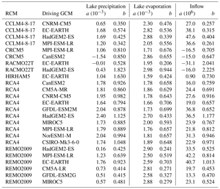
with the best estimate of Po, the distribution of the observed values, Pm the modelled values, and a and b calibration parameters. An overview of the a and b parameters generated per WB term for the different simulations can be found in Table D1 in the Appendix. The second method is the non-parametric quantile mapping method and is described in Sect. E in the Appendix.
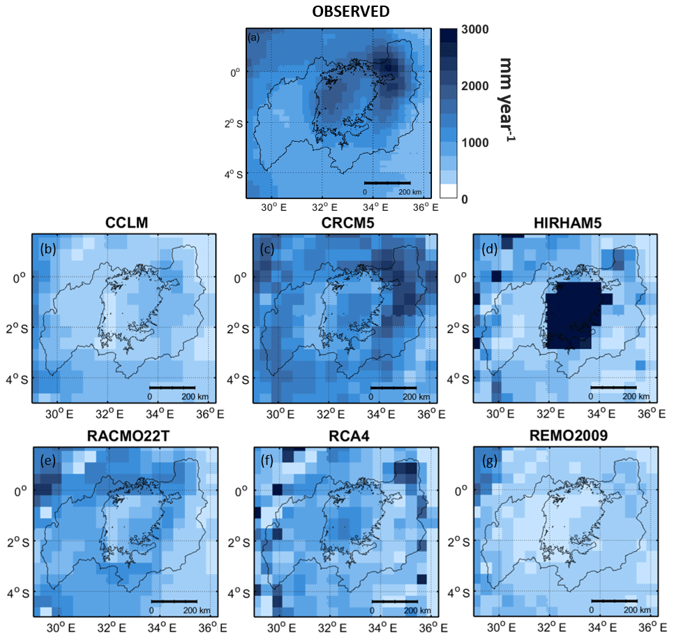
Figure 2Annual accumulated precipitation during the period 1993–2008 as derived from PERSIANN-CDR (a) the CORDEX evaluation simulations (b–g).
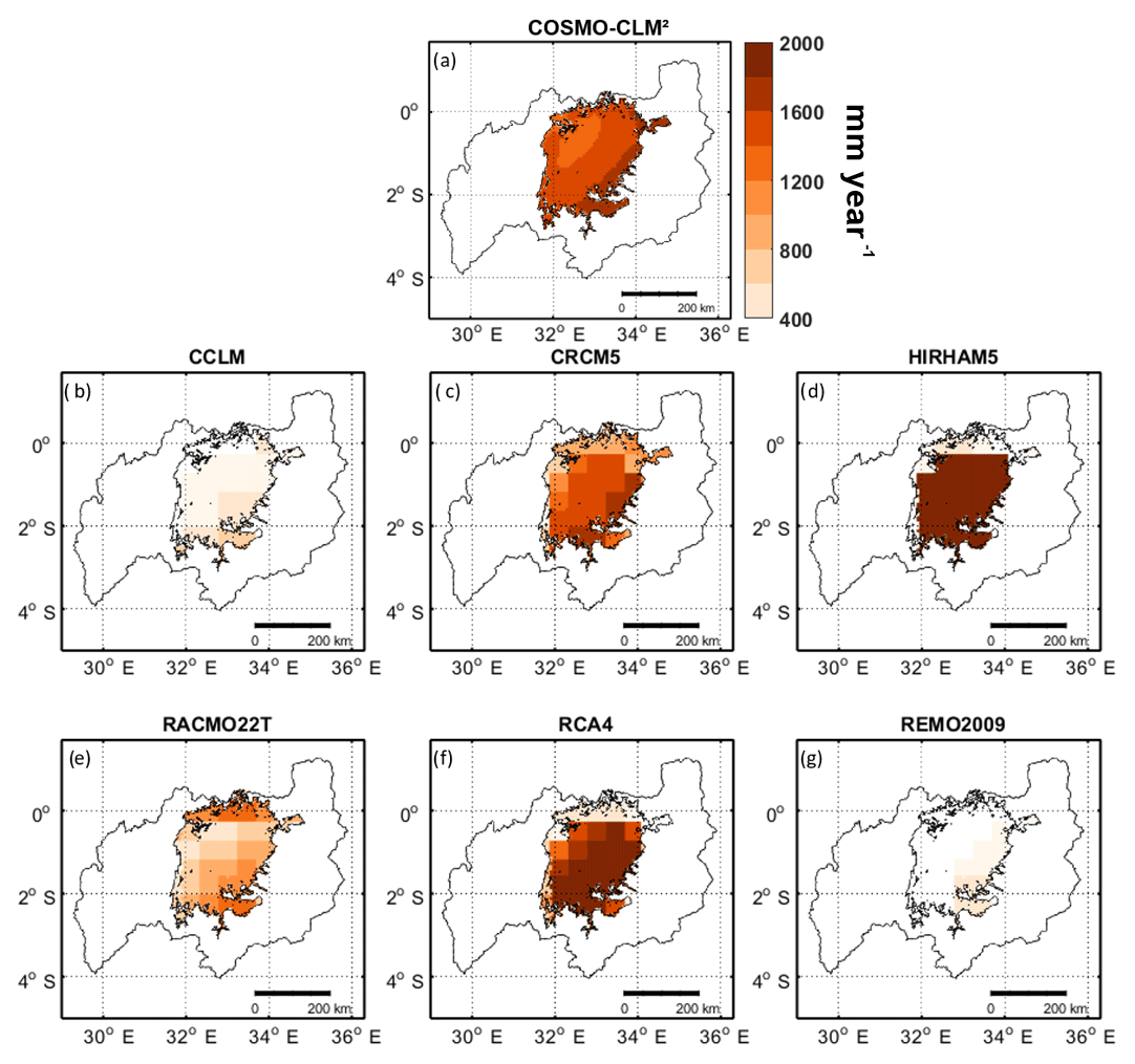
Figure 3Annual accumulated evaporation during the period 1993–2008 as derived from COSMO-CLM2 (a) the CORDEX evaluation simulations (b–g).

Figure 4Histograms of lake precipitation derived from the CORDEX evaluation simulations for the period 1993–2008 (observed distributions, derived from PERSIANN-CDR are indicated in grey).
3.1 Evaluation water balance simulations
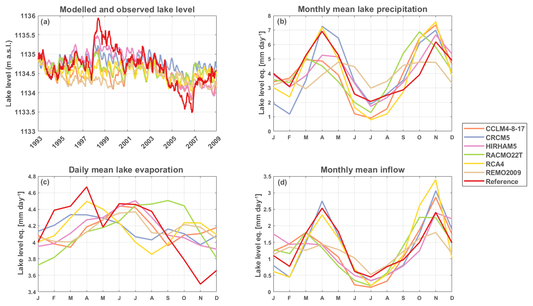
Results of the evaluation WBM runs are compared directly to the terms used in the observational WBM (Vanderkelen et al., 2018). Precipitation observations are retrieved from the Precipitation Estimation Remotely Sensed Information using Artificial Neural Networks – Climate Data Record (Ashouri et al., 2015). Evaporation is estimated from the latent heat flux output of the high-resolution reanalysis downscaling of the COSMO-CLM2 RCM (Thiery et al., 2015).
The modelled annual precipitation over the study area during the evaluation period (1990–2008) shows different spatial distributions (Fig. 2). Compared to the observed precipitation, the majority of the models (CCLM4-8-17, RACMO22T, RCA4 and REMO2009) underestimates the amount of lake precipitation up to −79 % compared to the reference. Only HIRHAM5 gives a large overestimation of precipitation over the lake of +78 % compared to the reference. The mean annual lake evaporation varies a lot among the models as well (Fig. 3). The evaporation amount is underestimated by CCLM4-8-17, RACMO22T and REMO2009 up to −71 % compared to the reference and overestimated by HIRHAM5 and RCA4 up to +39 %. Similar conclusions can be drawn from the comparison of the histograms of observed and simulated lake precipitation (Fig. 4). The difference between the distributions is also found for inflow and the resulting lake levels. The seasonal cycles of the WB terms – lake precipitation, evaporation and inflow (Fig. 5b, c and d) – show the same over- and underestimations compared to the observed values. This indicates that even RCM downscaling reanalysis data still entail important precipitation and evaporation biases. In most cases, the biases in precipitation and evaporation result in drifting lake levels (Fig. 5a). The overestimation of HIRHAM5 in the precipitation term is too large to be compensated by its overestimated evaporation term. Therefore, the modelled HIRHAM5 lake levels shows an unrealistic increase. The lake levels modelled with CCLM4-8-17, RACMO22T, RCA4 and REMO2009 show a large, unrealistic drop up to 13.3 m, which is mainly due to the underestimation of lake precipitation and inflow. Overall, only CRCM5 is able to represent the lake level within an acceptable range.
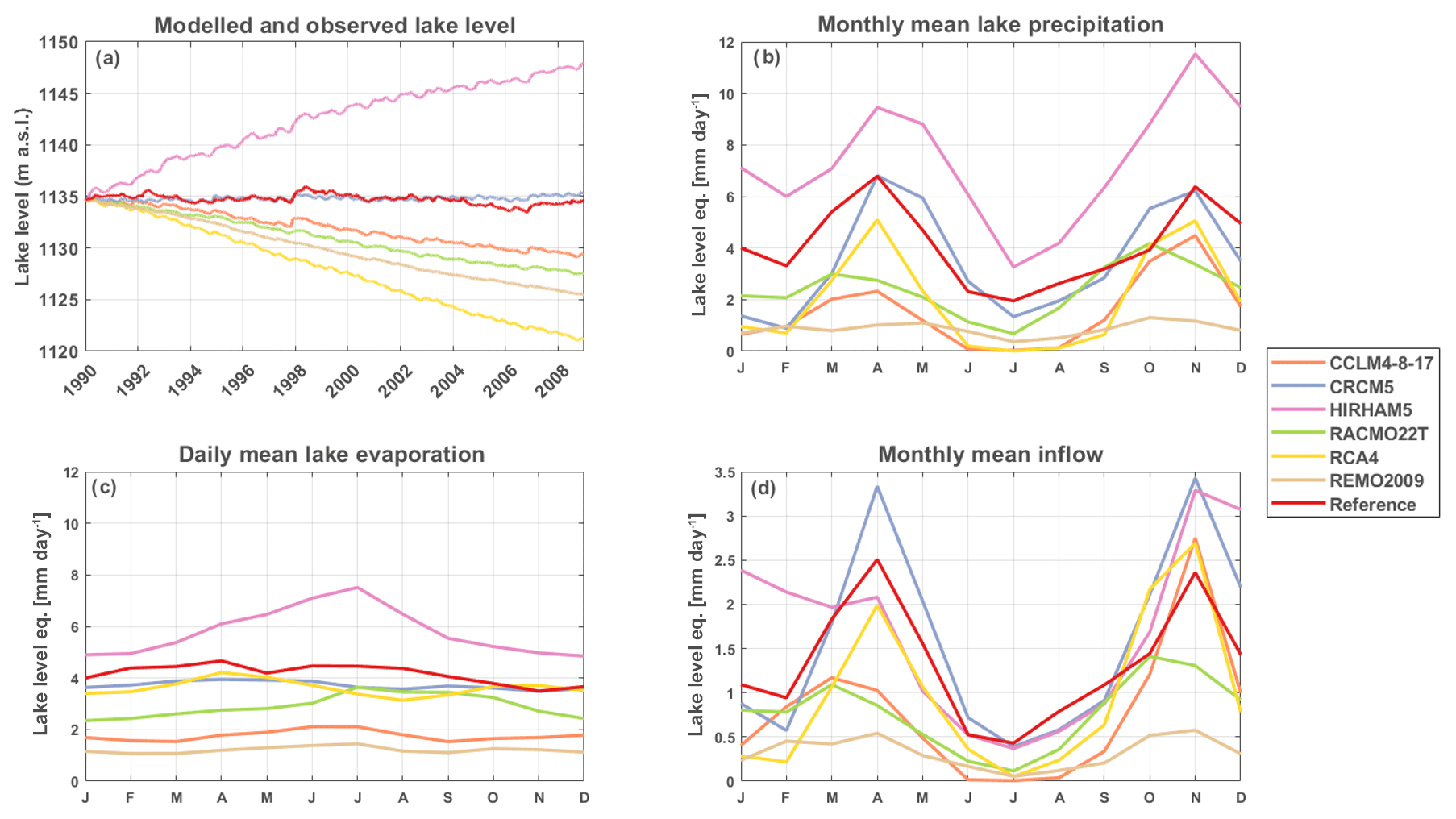
Figure 5Modelled lake levels (a), seasonal precipitation (b), evaporation (c) and inflow (d) according to the CORDEX evaluation simulations without bias correction. Note the different y axis scales.
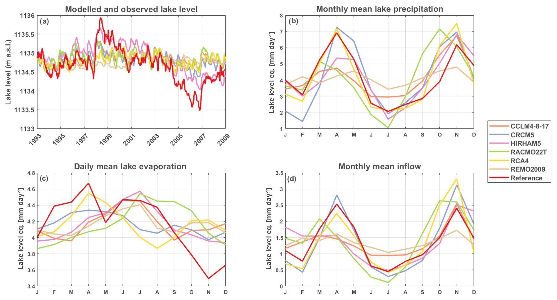
Figure 6Modelled lake levels (a), seasonal precipitation (b), evaporation (c) and inflow (d) according to the CORDEX evaluation simulations, bias corrected using parametric linear transformations. Note the different y axis scales.
3.2 Simulations with bias-corrected water balance terms
As only CRCM5 is able to close the WB and there are only two simulations following RCP 4.5 with this RCM available, it is not possible to base the analysis of lake level projections on an observationally constrained RCM ensemble. Therefore, we applied two bias-correction methods to be able to use all CORDEX simulations. After applying the linear parametric transformation on the CORDEX evaluation simulations, the seasonal cycle of the lake precipitation, lake evaporation and inflow term approximates the observations (Fig. 6). Consequently, the resulting lake levels lie within the range of observed lake levels. As the linear parametric bias-correction method provides a closed WB for all six RCMs, it is applied on the WB terms of the historical and future CORDEX simulations. Using the second bias-correction method, with empirical quantiles, also leads to WB closure. Applying this bias-correction method on the historical and future CORDEX simulations yields similar results as the linear parametric transformation. Therefore, only results from the linear parametric transformation are shown hereafter. Results with the empirical quantile bias-correction method are presented in the Appendix.
After applying the linear parametric bias correction, we quantified the future change of the three WB terms according to the three RCP scenarios for all simulations. This is achieved by computing the difference between the future (mean of the period 2071–2100) and the historical (mean of the period 1971–2000) simulations (Fig. 7). The climate change signal for lake precipitation differs between the simulations in every RCP scenario (Fig. 7a, b, c). For some simulations, lake precipitation demonstrates a strong decrease (e.g. CCLM4-8-17 driven by EC-EARTH, CRCM5 driven by CanESM2 and REMO2009 driven by EC-EARTH), while other simulations show an increase (e.g. RACMO22T driven by HadGEM2-ES and REMO2009 driven by CM5A-LR). The model simulations with a smaller increase or decrease also vary in sign. In contrast to lake precipitation, the lake evaporation signal is more consistent for the different simulations, with generally an increasing trend (Fig. 7d, e and f). The future changes in the inflow term are generally consistent as well and show an increase in inflow under all three RCP scenarios. As lake inflow is directly related to precipitation, the increase in inflow can be attributed to the increase in precipitation over the LVB. For all three WB terms, the width of the 95 % confidence intervals is larger for strong climate change signals.
The signs of the signals are broadly consistent with the signs of the original, non-bias-corrected WB terms (see Fig. E1 in the Appendix). The amplitude of the signals, however, generally decreases after applying the bias correction. This decrease is larger for the simulations with the more extreme signals, with important effects on the multi-model means.
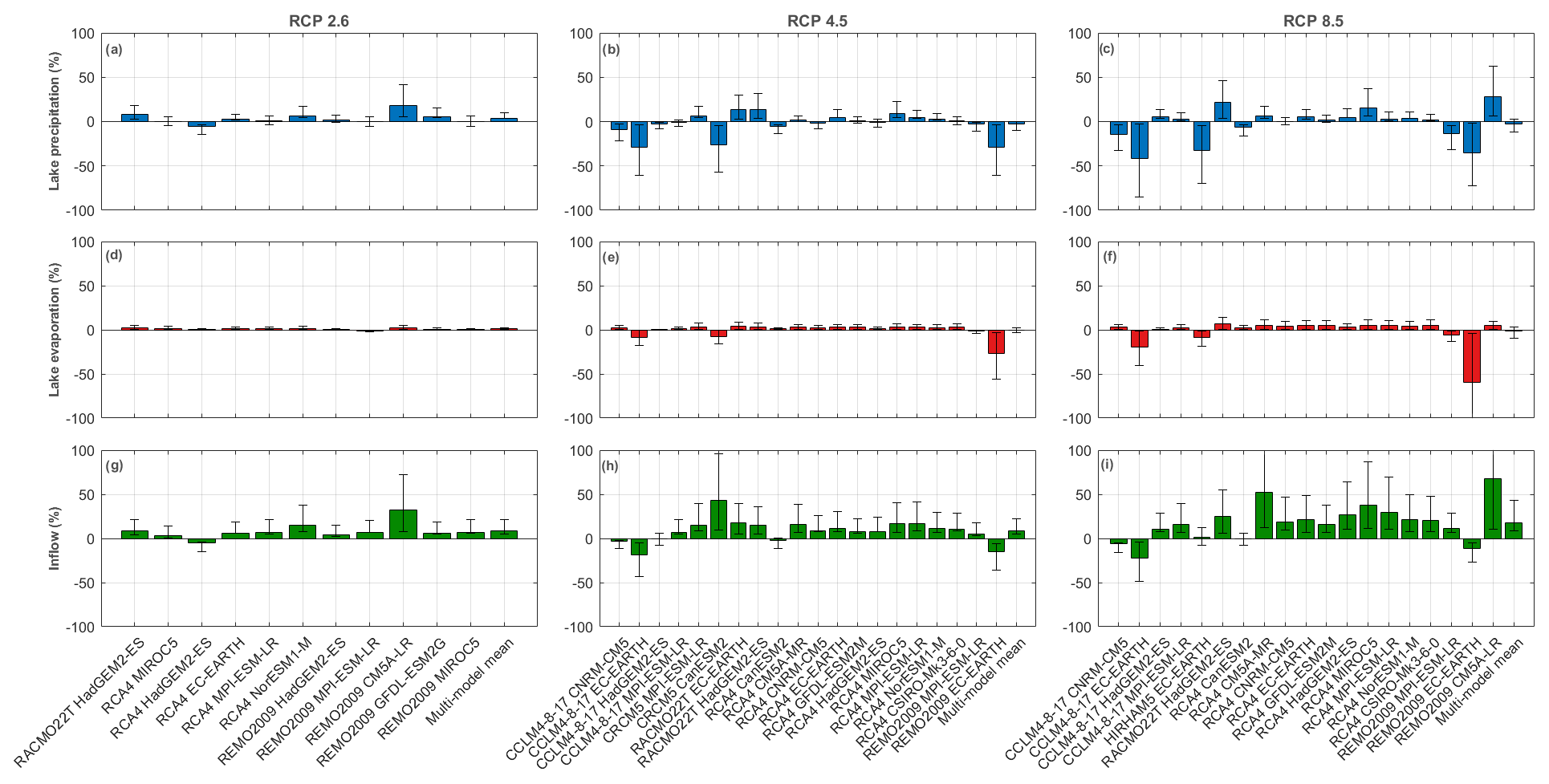
Figure 7Bar plots showing the relative projected climate chance following RCPs 2.6, 4.5 and 8.5 for lake precipitation (a–c), lake evaporation (d–f) and inflow (g–i) for the CORDEX simulations bias corrected with the linear parametric transformation. The climate change signal is defined as the mean difference between the future (2071–2100) and the historic (1971–2000) simulations. The whiskers indicate the 95 % confidence interval of the change based on the 30-year annual difference.
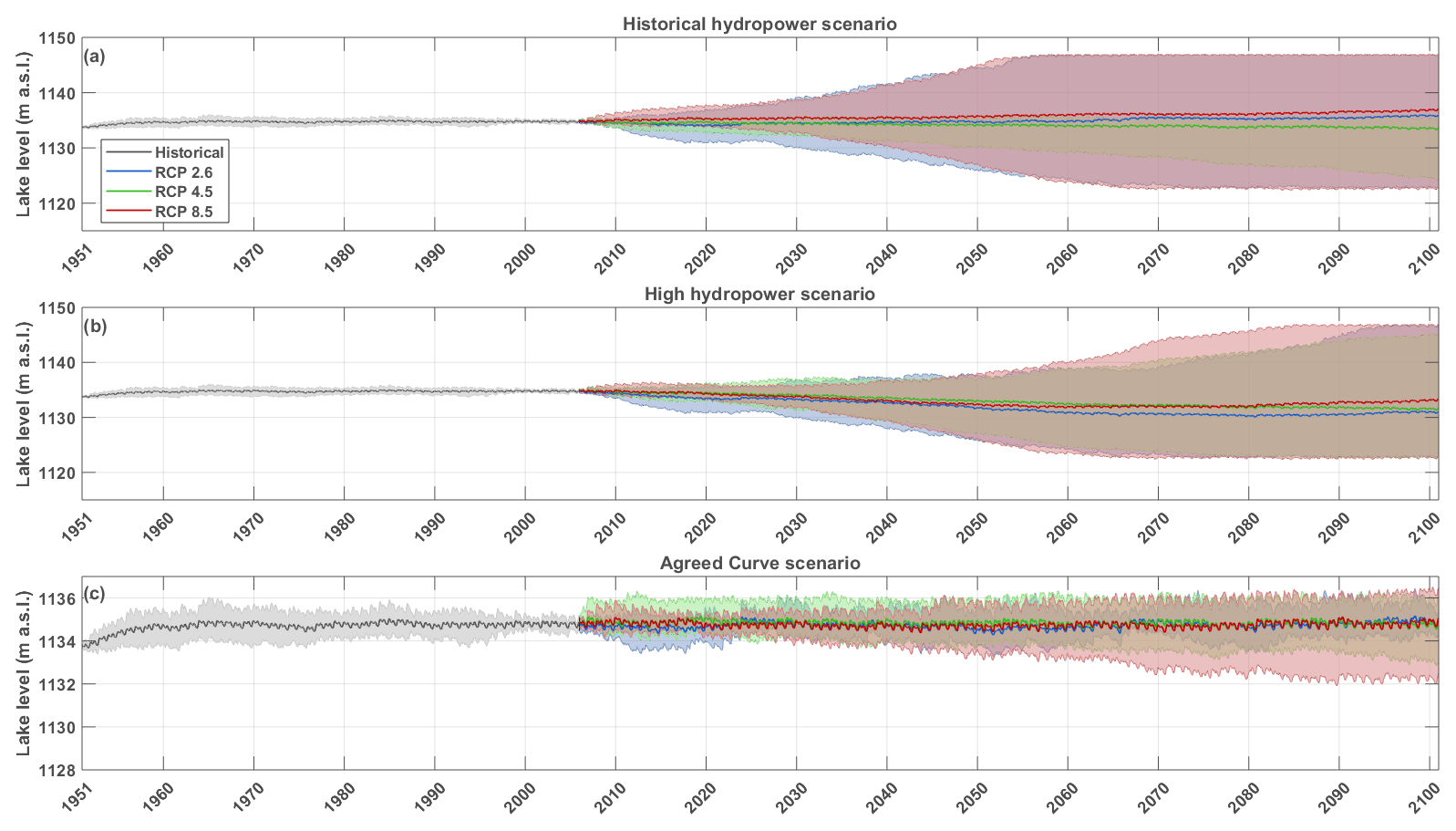
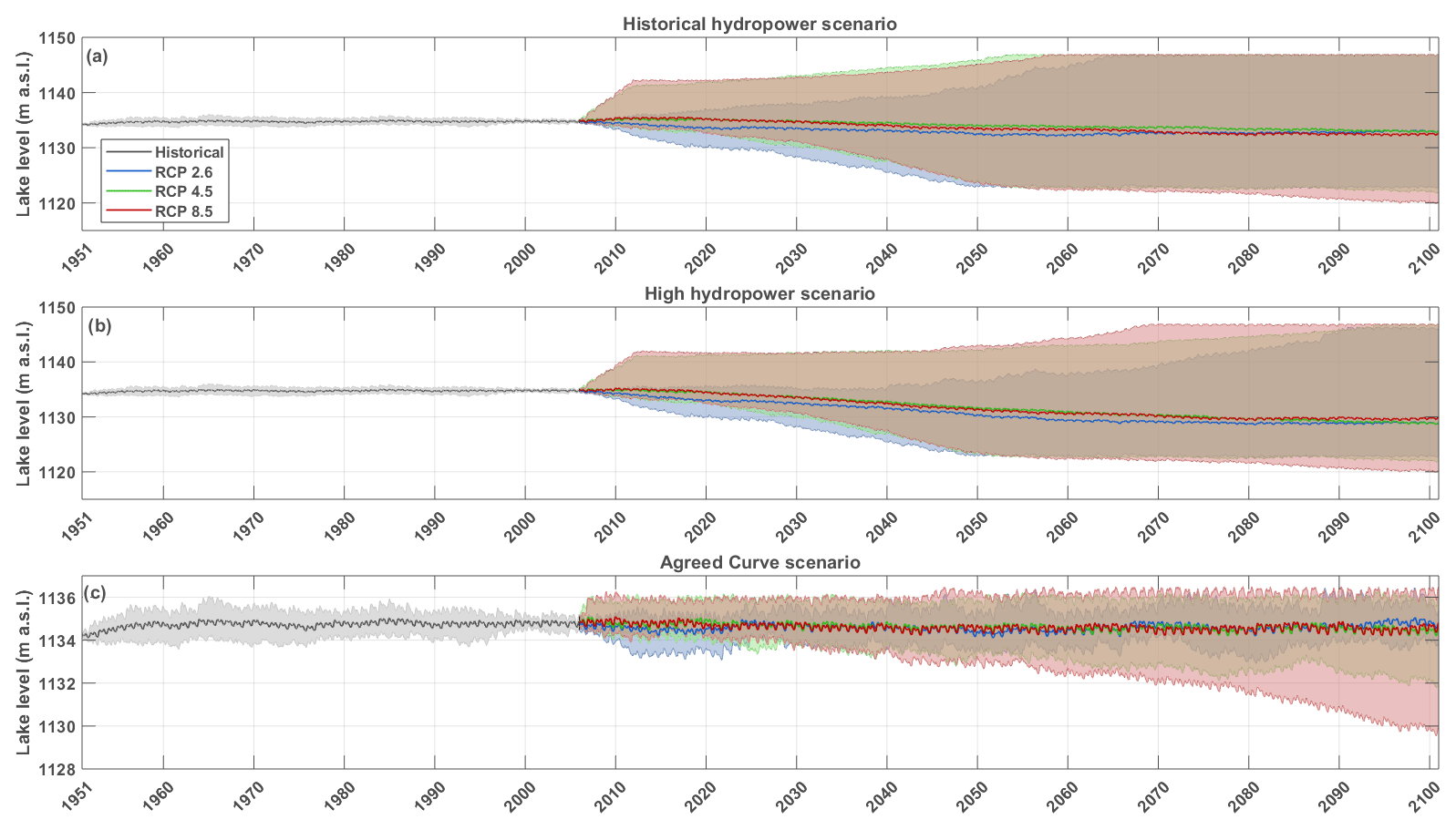
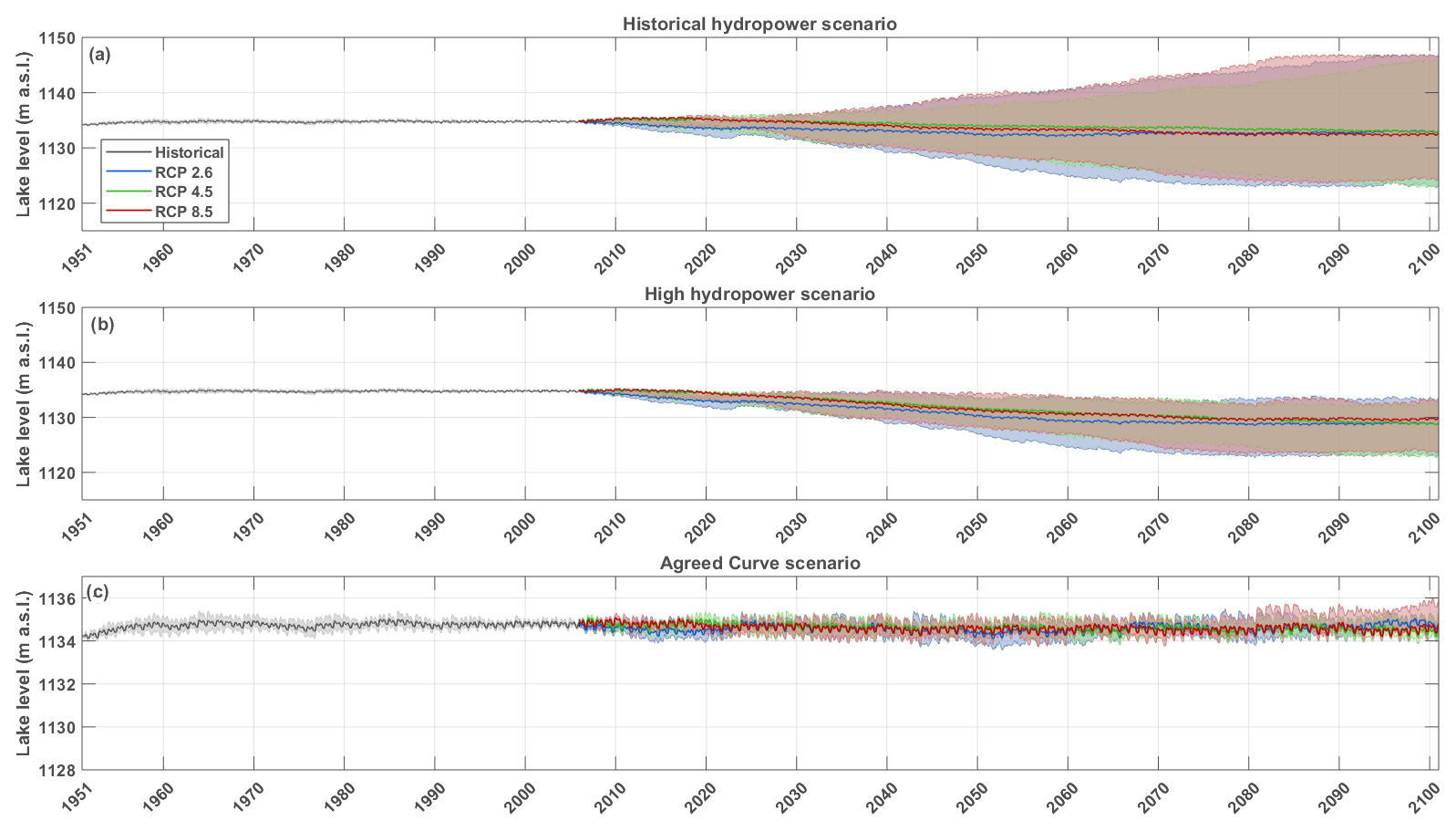
Figure 8Lake level projections for the historical HPP management scenario (Pel is 168 MW) (a), the high HPP management scenario (Pel is 247 MW) (b) and the Agreed Curve scenario (c). The solid line shows the ensemble means and the envelope the 5th–95th percentiles of the CORDEX ensemble simulations, bias corrected using the parametric linear transformation method. Note the different y axis scale for panel (c).
3.3 Future lake level and outflow projections
Lake level projections following different dam management scenarios are computed from the CORDEX simulations, bias corrected with a linear parametric transformation (Fig. 8). Future lake levels according to the constant lake level scenario are not represented in this figure, as they are constant at their 2006 level per definition. Under the historical HPP scenario, the ensemble mean projects a lake level increase of 1.03 m for RCP 2.6, 2.2 m for RCP 8.5 and a decline of −0.36 m for RCP 4.5 in 2100, compared to the 2006 level (Fig. 8a). The ensemble mean lake level projections thereby all stay within the observed range. The model uncertainty increases over time for three RCPs with an enveloped width ranging up to 24 m. The uncertainty range encompasses both rising and decreasing lake levels (e.g. up to +12 and −12 m in 2100 under RCP 8.5). The different simulations tend to diverge with a more or less constant ensemble mean as a result, as is shown by their interquartile range (Fig. C1 in the Appendix). Overall, lake level projections thus encompass large uncertainties within this management scenario. In the high HPP scenario the ensemble mean projections of the three RCPs project a decrease in lake level (−3.9 m for RCP 2.6, −3.2 m for RCP 4.5 and −1.5 m for RCP 8.5; Fig. 8b). The model uncertainty again increases with time for the three RCPs, consistent with the rising spread in the historical HPP management scenario.
In the Agreed Curve scenario, the outflow is adjusted every day based on the lake level of the previous day. In this scenario, the modelled lake levels stay within the range of the historical fluctuations and show no clear trend (Fig. 8c). The seasonal cycles in lake level are clearly visible in the ensemble mean. In 2100, the uncertainty has increased to 1.1 m for RCP 2.6, 3.1 m for RCP 4.5 and 3.9 m for RCP 8.5. It is not surprising that the lake level modelled with this scenario stays within the historical range, as the approximated WB equilibrium is maintained by adjusting the outflow based on the lake level on a daily basis. Moreover, the Agreed Curve relation between lake level and outflow is originally made to mimic natural outflow, accounting for the natural climate variability (Sene, 2000).

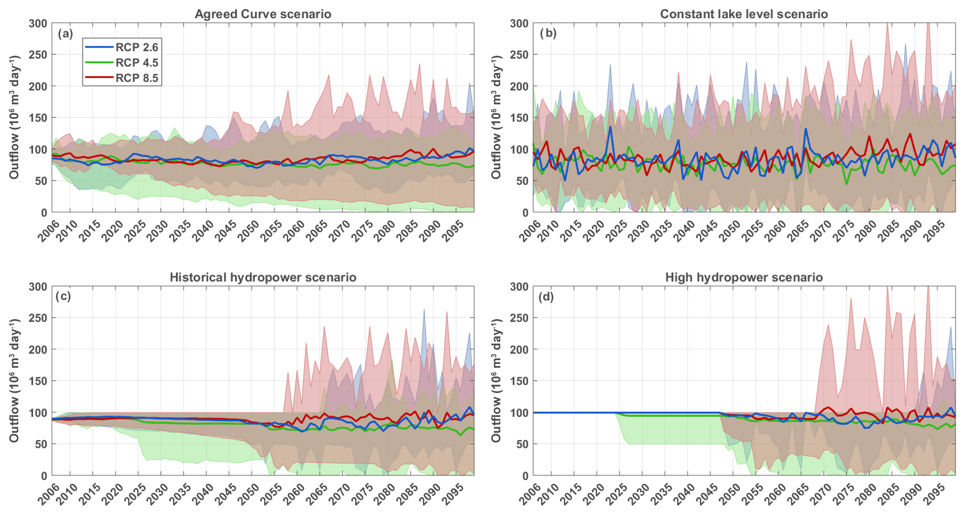
Figure 9Outflow projections (annual averaged) for the Agreed Curve scenario (a), the constant lake level scenario (b), the historical HPP management scenario (c) and the high HPP management scenario (d). The solid line shows the ensemble means and the envelope the 5th–95th percentiles of the CORDEX ensemble simulations, bias corrected using the parametric linear transformation method.
The outflow projections following the Agreed Curve scenario fluctuate around the historically observed outflow volume for RCPs 2.6 and 4.5. For RCP 8.5 the model projects a slight increase towards the end of the century, resulting in an averaged outflow volume being 6.7×10⁶ m3 day−1 (+7.6 %) higher than the historically observed outflow. This increase in outflow results from outflow volumes for some simulations that are larger than prescribed by the Agreed Curve, as the lake level for these simulations reaches the prescribed maximum lake level and all additional water is discharged. The uncertainty in the projections is therefore very large, ranging from 14×106 to 209×106 m3 day−1 for RCP 8.5, whereby the latter constitutes more than double the historically observed outflow (88×106 m3 day−1).
In the constant lake level scenario, the outflow volume varies following a spiky pattern (Fig. 9b). Since the outflow is altered each day to maintain a constant lake level given the precipitation, inflow and evaporation terms of that day, the outflow volume greatly varies on daily timescales with an average standard deviation of 172×106 m3 day−1. Fig. 9b therefore shows annually averaged daily outflow values. The three RCPs show no clear trend, but uncertainties range up to 253×106 m3 day−1. Fluctuating around a multi-model mean of 88.9×10⁶ m3 for RCP 2.6, 90.3×10⁶ m3 for RCP 4.5 and 95.5×10⁶ m3 for RCP 8.5, annual average outflow volumes are higher than historical outflow, with an average outflow volume of 88×106 m3 day−1, measured from 1950 until 2006.
Finally, outflow volumes following the historical HPP scenario decrease slightly until roughly 2055, whereas outflow volumes following the high HPP scenario remain constant until 2055 (Fig. 9c and d). Afterwards, the ensemble mean outflow projections start to diverge and uncertainties strongly increases. From this moment, most lake level projections reach the imposed minimum or maximum levels (Sect. 2.3). No outflow is released for projections which drop to the minimum level, while all additional water is discharged for lake levels which reach the maximum level. Consequently, with outflow volumes reaching these extremes, it is not possible to maintain a constant hydropower supply, despite the management scenario being designed for this aim.
4.1 Model quality and projected changes
None of the RCMs, except for CRCM5, are able to provide reliable estimations of the WB terms in the LVB (Figs. 4 and 5). Endris et al. (2013) found that most RCMs simulate the main precipitation features reasonably well in East Africa. Over the whole CORDEX-Africa domain, all RCMs capture the main elements of the seasonal mean precipitation distribution and its cycle, but also significant biases are present in individual models depending on season and region (Kim et al., 2014; Nikulin et al., 2012). Here, a specific region is investigated wherein lakes act as main driving features of the regional climate (Docquier et al., 2016; Thiery et al., 2015, 2016, 2017). Therefore, model performance is primarily determined by how lakes are resolved in the models. A correct representation of lake surface temperatures in the models is crucial to account for the lake–climate interactions and associated mesoscale circulations (Stepanenko et al., 2013; Thiery et al., 2014a, b). The good performance of CRCM5 can be attributed to the presence of the lake model FLake, ensuring a realistic representation of lake surface temperatures, while the other models have no lake model embedded. The fact that RCA4, which also uses FLake as lake model, gives no accurate representation of the WB terms in the LVB is most likely due to other model biases apart from the lake model.
Thiery et al. (2016) performed high-resolution simulations (∼7 km grid spacing) with the coupled land–lake–atmosphere model COSMO-CLM2 under RCP 8.5 over the LVB. In these simulations, the precipitation shows a decrease of −7.5 % towards the end of the century over the lake surfaces of the African Great Lake region, which is a higher decrease than found in this study (−2.3 %). The increase in lake evaporation following RCP 8.5 according to Thiery et al. (2016) (+142 mm year−1) confirms the sign of the evaporation signal of most CORDEX simulations of this study (Fig. E1f). However, the effect is not visible in the bias-corrected multimodel mean (−0.07 mm year−1), which results from the negative signal of three CORDEX simulations (Fig. E1f). While COSMO-CLM² generally outperforms CORDEX-Africa simulations, these simulations are only available in time slices and could therefore not be used to drive the WBM.
The decrease in lake precipitation for RCPs 4.5 and 8.5 (respectively −2.5 % and −2.3 %) is not visible in the lake level projections following the Agreed Curve or the HPP scenarios. This is due to the fact that the decrease in lake precipitation is largely compensated in the total WB by the increase in lake inflow, which is determined by the increase in precipitation over the LVB. In the bias-corrected simulations using the linear parametric transformation, the deficit in lake precipitation is compensated for 184 % (RCP 4.5) and 450 % (RCP 8.5) by an increase in inflow. In RCP 2.6, this effect is not present.
4.2 Water management and climate change
The analysis reveals that the management scenario has an important influence on the future lake levels and outflow volumes. The physical lake level constraint means that the effect of unsustainable management scenarios is reflected in the outflow volumes, which become highly variable once the lake level limit is reached. In both constant HPP scenarios, various simulations reach these limits, leading to very high or almost no outflow anymore, and a hydropower production which does not meet the goal for which it was designed. The multi-model mean lake level projections following these management scenarios appear sustainable, but are the result of averaging two branches of drifting lake levels, as illustrated by the interquartile range being large compared to the Agreed Curve (see Fig. C1 in the Appendix). Lake levels diverge towards their limits, leading to extreme situations where the lake extent is altered substantially, causing various impacts along the shoreline, such as reduced accessibility to fishing grounds and harbours located in shallow bays. Therefore, the dam management scenarios aiming at constant hydropower production are not sustainable. Furthermore, to meet the goal of a constant lake level, the outflow volumes have to be highly variable, which is not realistic if hydropower generation is pursued. Therefore the constant lake level scenario can also be qualified as unsustainable.
If the released dam outflow follows the Agreed Curve, the lake level will reflect the climatic conditions and it will fluctuate within its natural range. Moreover, the corresponding outflow following the multi-model mean also stays within the observed range. However, the uncertainties in the outflow simulations reach up to 229 % of the projected multi-model mean, highlighting that future lake level trajectories may strongly differ even under a single climate change realization. This has important implications for the potential hydropower generation and water availability downstream: while the lowest projected outflow volumes close to zero inhibit hydropower potential and exacerbate hydrological drought in the White Nile, increased outflow volumes could lead to more flooding downstream. Hence, strong changes in downstream water availability may occur in the next decades even if dam managers adhere to the Agreed Curve. Nevertheless, considering the multi-model mean, the Agreed Curve scenario can be denoted as a sustainable management scenario. However, violations against the prescribed outflow can have important consequences for the lake levels, as shown by the observed drop in lake level in 2004–2005, which was 48 % attributable to an enhanced dam outflow (Vanderkelen et al., 2018). In Uganda, hydropower provides up to 90 % of the electricity generated (Adeyemi and Asere, 2014). There is a rapidly growing gap between electricity supply and a rising demand, as the electricity consumption per capita in Uganda is among the lowest in the world. The Kiira and Nalubaale hydropower stations, managing Lake Victoria's outflow, are the largest power generators in the country (Adeyemi and Asere, 2014). The third largest capacity is provided by the new Bujagali hydropower dam located 8 km downstream of Lake Victoria. Therefore, operations at those dams will become even more important in the future. If there are again violations against the Agreed Curve because of the increasing hydropower demand, this may have substantial consequences for the future evolution of the lake level. A relatively stable lake level is, however, necessary for local water availability providing resources to the 30 million people living in its basin and to the 200 000 fisherman operating from its shores (Semazzi, 2011).
Within each management scenarios, the climate model uncertainty appears to be larger than the uncertainty related to the emission scenario. This could be seen by the large spread around the multi-model mean and the coinciding RCP curves and spread (Figs. 8 and 9). The spread according to the RCP 2.6 scenario is the smallest. This scenario contains only 11 simulations, while there are 19 simulations following RCP 4.5 and 17 simulations following RCP 8.5. The future projections provide no clear differentiation between the three RCP scenarios, indicating that uncertainties associated with the model deficiencies and initial conditions play a more important role. Therefore, to further refine lake level projections presented in this study, it is of vital importance to account for model deficiencies and natural variability.
Apart from the large climate model uncertainties, this approach using the WB model has some other shortcomings. First, we do not account for future land cover changes in the inflow calculations, as a static land cover map for the year 2000 is used (Vanderkelen et al., 2018). Changes in land cover are, however, very important in future simulations, as they affect the curve number and therefore the amount of runoff (Ryken et al., 2014). Moreover, future changes in land use could induce changes in precipitation in tropical regions (Akkermans et al., 2014; Lejeune et al., 2015). Second, the employed management scenarios are based on three simple assumptions. The management scenario exerts a major influence on future lake level fluctuations and future lake levels appeared to be sustainable only if the Agreed Curve is followed. As the importance of dam management in response to rising hydropower demand increases, more sophisticated management scenarios accounting for the rising hydropower demand could be developed and examined for their ability to preserve historical lake level fluctuations.
In this second part of a two-paper series, a water balance model (WBM) developed for Lake Victoria is forced with climate projections from the COordinated Regional Climate Downscaling Experiment (CORDEX) ensemble following three representative concentration pathways (RCPs 2.6, 4.5 and 8.5). Lake level fluctuations are projected up to 2100 using four different dam management scenarios, which emerge from three policy objectives.
This study identified the following key messages. (i) RCMs incorporated in the CORDEX ensemble are typically not able to reproduce Lake Victoria's WB, and therefore require bias correction. Applying the bias correction closes the WB and results in realistically simulated lake levels. (ii) The projected decrease in lake precipitation under RCPs 4.5 and 8.5 is compensated by an increase in lake inflow, which is directly determined by precipitation over the Lake Victoria Basin. (iii) The choice of management strategy will determine whether the lake level evolution remains sustainable or not. Idealized dam management pursuing a constant hydropower production (electricity policy objective) leads to unsustainable lake levels and outflow fluctuations. The management scenario in which the lake level is kept constant, targeting a reliable navigation policy, leads to highly variable outflow volumes, which is not realistic in terms of hydropower production. (iv) When outflow is managed following the Agreed Curve, mimicking natural outflow pursuing environmental policy targets, the evolution of lake level and outflow remains sustainable for most realizations. (v) The outflow projections following the Agreed Curve, however, encompass large uncertainties, ranging from 14×106 to 209×106 m3 day−1 (up to 229 % of the historically observed outflow). Although the multi-model mean projected lake levels demonstrate no clear trend, these large uncertainties show that even if the Agreed Curve is followed, future lake levels and outflow volumes could potentially rise or drop drastically, with profound potential implications for local hydropower potential and downstream water availability. (vi) Next to the management scenario, we found that climate model uncertainty (RCM-GCM combination) is larger than the uncertainty related to the emission scenario.
In this study, we provide the first indications of potential consequences of climate change for the water level of Lake Victoria. The large biases and uncertainties present in the projections stress the need for an adequate representation of lakes in RCMs to be able to make reliable climate impact studies in the African Great Lakes region. Finally, the evolution of future lake levels of Lake Victoria are primarily determined by the decisions made at the dam. Therefore, the dam management of Lake Victoria is of major concern to ensure the future of the people living in the basin, the future hydropower generation and water availability downstream.
The water balance model code is publicly available at https://github.com/VUB-HYDR/2018_Vanderkelen_etal_HESS_ab (Vanderkelen, 2018). The qmap R package is available on the Comprehensive R Archive Network (https://cran.r-project.org/, Gudmundsson, 2018). Data from the COordinated Regional Climate Downscaling Experiment (CORDEX) Africa framework is available at http://cordex.org/data-access/esgf/ (CORDEX, 2018).
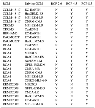
The CORDEX ensemble simulations used in this study are listed in Table A1. From all available simulations, the simulation of HIRHAM5 driven by EC-EARTH following RCP 4.5 is not used because it exhibits discrepancies between its historical and future simulation. These discrepancies are nonphysical and inhibit the application of a bias correction.
Table A1Overview of the different CORDEX simulations and their availability (Y: yes, N: no). (*data not used because of discrepancy between historical and future simulation).
Not all simulations from the CORDEX ensemble have the same number of days. As a fixed number of days is a necessary condition to compare the WBM simulations, a correction was applied on the daily WB terms of some simulations.
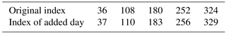
First, simulations driven by HadGEM2-ES (CCLM4-8-17, RACMO22T, RCA4, REMO2009), have 30-day months and only go until 2099. To account for the missing days, 5 extra days are added for every 72 days in the year, starting after the 36th day. The index of these 5 extra days within each year are given in Table B1. The added days are the average of the respective WB terms during the previous and next day. In addition, we accounted for the fact that these model simulations do not include the year 2100, by repeating the year 2099. The simulations with HadGEM2-ES for RCP 4.5 have no December month in the year 2099. This is also the case for the HadGEM2-ES CCLM4-8-17 simulation for RCP 8.5. In both cases, December 2099 is added by repeating the month November of the same year.
Finally, in all simulations that do not account for leap years (RCMs driven by CanESM2, NorESM1-M, MIROC5, GFDL-ESM2M, CM5A-MR and CSIRO-Mk3-6-0), an extra day in the leap years is added by taking the average WB term value of the days corresponding to the 28 February and the 1 March. Overall, compared to the total number of days of the future projections (34 698 days), we note that corrections on single days (up to 888 days depending on the simulations) have a little influence on the outcomes of this study.
The interquartile range of the lake level projections (Fig. C1) compared with their 5th and 95th percentile envelope shows a large decrease in uncertainty range for outflow following the Agreed Curve, while the uncertainty following the HPP management scenarios knows a smaller decrease.
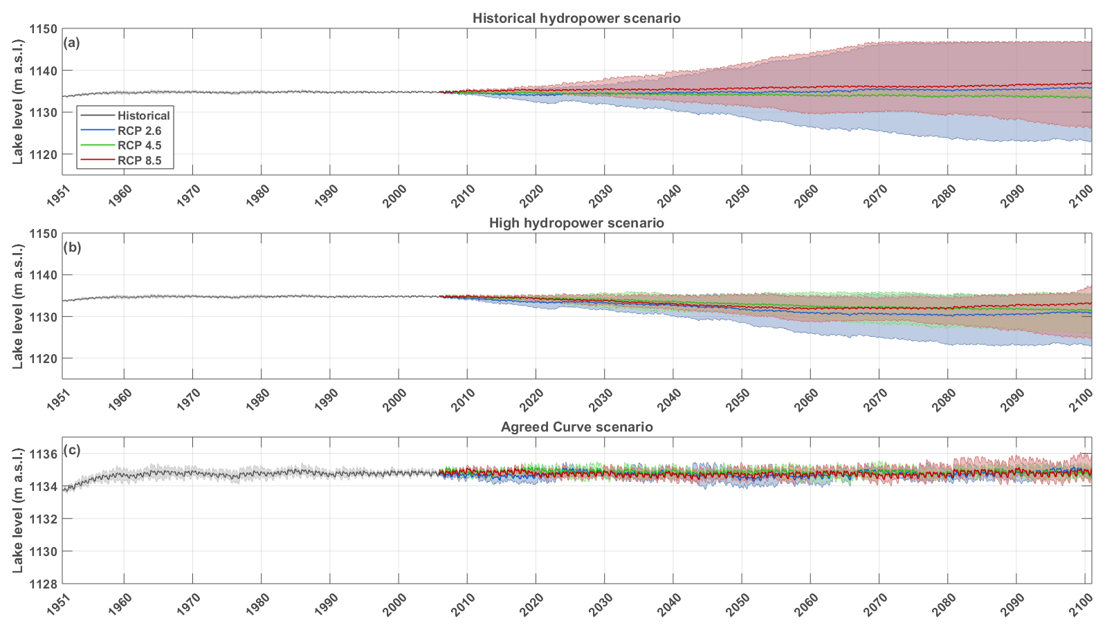
Table D1 shows the a and b calibration parameters for the different CORDEX simulations used in the linear parametric transformation to bias correct the lake precipitation, evaporation and inflow terms of the WB.
Table D1Parameters a and b of the linear parametric transformation of the WB terms for the different CORDEX simulations (Eq. 5).
Next to the bias-correction method using a linear parametric transformation (see Sect. 2.4), WB closure was adhered with a second method which is the non-parametric quantile mapping method, a common approach for statistical transformation (Boé et al., 2007; Panofsky and Brier, 1968; Themeßl et al., 2011, 2012; Wood et al., 2004). Following Gudmundsson et al. (2012) and Boé et al. (2007), this method uses the cumulative density function (CDF) based on the empirical quantiles from the observed variable to transform the modelled variable. First, the CDFs of the three WB terms following each historical simulation in the overlapping period (the reference simulations) are matched with the cumulative density function of the WB terms from the observational WBM (observations). This generates a correction function, relating the quantiles of both distributions. Next, this correction function is used to unbias the WB term simulations for the whole simulation period quantile by quantile (Boé et al., 2007).
When a bias correction based on empirical quantiles is used, very similar results are found (compare Figs. E2, E3, E4 and E6). Based on this, we conclude that the bias-correction methods has very little effect on the results presented in this study.

Figure E1Bar plots showing the relative projected climate chance following RCPs 2.6, 4.5 and 8.5 for lake precipitation (a–c), lake evaporation (d–f) and inflow (g–i) for the CORDEX simulations without bias correction. The climate change signal is defined as the difference between the future (2071–2100) and the historical (1971–2000) simulations. The whiskers indicate the 95 % confidence interval of the change based on the 30-year annual difference.
In this study, applying a bias correction on the WB terms of the CORDEX simulations was necessary to be able to make lake level and outflow projections, as subsetting is not possible. RCMs are often bias corrected, as their simulations inhibit errors (Christensen et al., 2008; Lange, 2018; Maraun et al., 2010; Teutschbein and Seibert, 2013; Themeßl et al., 2012). Both linear parametric transformation and the quantile mapping bias-correction methods are used. The advantage of the first is the simplicity and transparency of the method (Teutschbein and Seibert, 2013). The quantile mapping method, on the other hand, is a non-parametric method and is able to correct for errors in variability as well (Themeßl et al., 2011). Yet, no substantial differences could be noted between the resulting projections of both methods, which supports that there is no single optimal way to correct for RCM biases (Themeßl et al., 2011). It is, however, important to consider the limitations concerning the bias-correction methods. In both methods, each WB term is corrected independently, whereas biases may not be independent among the terms, which may be important in the context of climate change (Boé et al., 2007). The consistency between the variables could be preserved by using a more sophisticated method using a multivariate bias correction (Cannon, 2017; Vrac and Friederichs, 2015). However, Maraun et al. (2017) showed that bias correction could lead to improbable climate change signals and cannot overcome large model errors.

IV, NPMvL and WT designed the study. IV performed the analysis and wrote the manuscript. All authors commented on the manuscript.
The authors declare that they have no conflict of interest.
This article is part of the special issue “Modelling lakes in the climate system (GMD/HESS inter-journal SI)”. It is a result of the 5th workshop on “Parameterization of Lakes in Numerical Weather Prediction and Climate Modelling”, Berlin, Germany, 16–19 October 2017.
We acknowledge the CLM-community (https://www.clm-community.eu/, last
access: 16 October 2018) for developing COSMO CLM2 and making the model
code available. Computational resources and services used for the
COSMO-CLM2 simulations were provided by the VSC (Flemish Supercomputer
Centre), funded by the Hercules Foundation and the Flemish Government
department EWI. In addition, we are grateful to the World Climate Research
Programme (WRCP) for initiating and coordinating the CORDEX-Africa initiative
and to the modelling centres for making their downscaling results publicly
available through ESGF. Wim Thiery was supported by an ETH Zurich
postdoctoral fellowship (Fel-45 15-1). The Uniscientia Foundation and the ETH
Zurich Foundation are thanked for their support to this
research.
Edited by: Miguel
Potes
Reviewed by: two anonymous referees
Adeyemi, K. O. and Asere, A. A.: A Review of the Energy Situation in Uganda, International Journal of Scientific and Research Publications, 4, 2250–3153, https://doi.org/10.1260/014459806779398811, 2014. a, b, c
Akkermans, T., Thiery, W., and Van Lipzig, N. P. M.: The Regional Climate Impact of a Realistic Future Deforestation Scenario in the Congo Basin, J. Climate, 27, 2714–2734, https://doi.org/10.1175/JCLI-D-13-00361.1, 2014. a
Ashouri, H., Hsu, K. L., Sorooshian, S., Braithwaite, D. K., Knapp, K. R., Cecil, L. D., Nelson, B. R., and Prat, O. P.: PERSIANN-CDR: Daily precipitation climate data record from multisatellite observations for hydrological and climate studies, B. Am. Meteorol. Soc., 96, 69–83, https://doi.org/10.1175/BAMS-D-13-00068.1, 2015. a
Boé, J., Terray, L., Habets, F., and Martin, E.: Statistical and dynamical downscaling of the Seine basin climate for hydro-meteorological studies, Int. J. Climatol., https://doi.org/10.1002/joc.1602, 27, 1643–1655, 2007. a, b, c, d
Cannon, A. J.: Multivariate quantile mapping bias correction: an N-dimensional probability density function transform for climate model simulations of multiple variables, Clim. Dynam., 50, 31–49, https://doi.org/10.1007/s00382-017-3580-6, 2017. a
Christensen, J. H., Boberg, F., Christensen, O. B., and Lucas-Picher, P.: On the need for bias correction of regional climate change projections of temperature and precipitation, Geophys. Res. Lett., 35, 20709, https://doi.org/10.1029/2008GL035694, 2008. a
CORDEX-Africa simulation data: available at http://www.cordex.org/data-access/esgf/, last access: 16 October 2018.
Davin, E. L., Maisonnave, E., and Seneviratne, S. I.: Is land surface processes representation a possible weak link in current Regional Climate Models?, Environ. Res. Lett, 11, 074027, https://doi.org/10.1088/1748-9326/11/7/074027, 2016. a
Deconinck, S.: Security as a threat to development: the geopolitics of water scarcity in the Nile River basin, Focus Paper, Royal High Insitute for Defence, Brussels, Belgium, 2009. a
Di Baldassarre, G., Elshamy, M., Van Griensven, A., Soliman, E., Kigobe, M., Ndomba, P., Mutemi, J., Mutua, F., Moges, S., Xuan, Y., Solomatine, D., and Uhlenbrook, S.: Future hydrology and climate in the River Nile basin: a review, Hydrolog. Sci. J., 56, 199–211, https://doi.org/10.1080/02626667.2011.557378, 2011. a
Docquier, D., Thiery, W., Lhermitte, S., and van Lipzig, N. P. M.: Multi-year wind dynamics around Lake Tanganyika, 47, 3191–3202, https://doi.org/10.1007/s00382-016-3020-z, 2016. a
Endris, H. S., Omondi, P., Jain, S., Lennard, C., Hewitson, B., Chang'a, L., Awange, J. L., Dosio, A., Ketiem, P., Nikulin, G., Panitz, H. J., Büchner, M., Stordal, F., and Tazalika, L.: Assessment of the performance of CORDEX regional climate models in simulating East African rainfall, J. Climate, 26, 8453–8475, https://doi.org/10.1175/JCLI-D-12-00708.1, 2013. a, b
Giorgi, F., Jones, C., and Asrar, G. R.: Addressing climate information needs at the regional level: The CORDEX framework, World Meteorological Organization Bulletin, 58, 175–183, 2009. a
Gudmundsson, L., Bremnes, J. B., Haugen, J. E., and Engen-Skaugen, T.: Technical Note: Downscaling RCM precipitation to the station scale using statistical transformations – a comparison of methods, Hydrol. Earth Syst. Sci., 16, 3383–3390, https://doi.org/10.5194/hess-16-3383-2012, 2012. a, b
Gudmundsson, L.: qmap R package, available at: https://cran.r-project.org/web/packages/qmap/index.html, last access: 16 October 2018.
Hernández-Díaz, L., Laprise, R., Laxmi, S., Martynov, A., Winger, K., and Dugas, B.: Climate simulation over CORDEX Africa domain using the fifth-generation Canadian Regional Climate Model (CRCM5), Clim. Dynam., 40, 1415–1433, https://doi.org/10.1007/s00382-012-1387-z, 2012. a
Kent, C., Chadwick, R., and Rowell, D. P.: Understanding uncertainties in future projections of seasonal tropical precipitation, J. Climate, 28, 4390–4413, https://doi.org/10.1175/JCLI-D-14-00613.1, 2015. a, b
Kim, J., Waliser, D. E., Mattmann, C. A., Goodale, C. E., Hart, A. F., Zimdars, P. A., Crichton, D. J., Jones, C., Nikulin, G., Hewitson, B., Jack, C., Lennard, C., and Favre, A.: Evaluation of the CORDEX-Africa multi-RCM hindcast: Systematic model errors, Clim. Dynam., 42, 1189–1202, https://doi.org/10.1007/s00382-013-1751-7, 2014. a, b, c
Kizza, M. and Mugume, S.: The Impact of a Potential Dam Break on the Hydro Electric Power Generation: Case of: Owen Falls Dam Break Simulation, Uganda, in: International Conference on Advances in Engineering and Technology, edited by: Mwakali, J. and Taban-Wani, G., 711–722, Entebbe, Uganda, 2006. a
Koch, H., Liersch, S., and Hattermann, F. F.: Integrating water resources management in eco-hydrological modelling, Water Sci. Technol., 67, 1525–1533, https://doi.org/10.2166/wst.2013.022, 2013. a
Kull, D.: Connections Between Recent Water Level Drops in Lake Victoria, Dam Operations and Drought, Daniel Kull, Nairobi, available at: https://www.internationalrivers.org/sites/default/files/attached-files/full_report_pdf.pdf (last access: 19 October 2018), 2006. a, b
Lange, S.: Bias correction of surface downwelling longwave and shortwave radiation for the EWEMBI dataset, Earth Syst. Dynam., 9, 627–645, https://doi.org/10.5194/esd-9-627-2018, 2018. a
Lejeune, Q., Davin, E. L., Guillod, B. P., and Seneviratne, S. I.: Influence of Amazonian deforestation on the future evolution of regional surface fluxes, circulation, surface temperature and precipitation, Clim. Dynam., 44, 2769–2786, https://doi.org/10.1007/s00382-014-2203-8, 2015. a
Lyon, B. and Dewitt, D. G.: A recent and abrupt decline in the East African long rains, Geophys. Res. Lett., 39, 1–5, https://doi.org/10.1029/2011GL050337, 2012. a
Maraun, D., Wetterhall, F., Ireson, A. M., Chandler, R. E., Kendon, E. J., Widmann, M., Brienen, S., Rust, H. W., Sauter, T., Themel, M., Venema, V. K., Chun, K. P., Goodess, C. M., Jones, R. G., Onof, C., Vrac, M., and Thiele-Eich, I.: Precipitation downscaling under climate change: Recent developments to bridge the gap between dynamical models and the end user, Rev. Geophys., 48, 2009RG000314, https://doi.org/10.1029/2009RG000314, 2010. a
Maraun, D., Shepherd, T. G., Widmann, M., Zappa, G., Walton, D., Gutiérrez, J. M., Hagemann, S., Richter, I., Soares, P. M., Hall, A., and Mearns, L. O.: Towards process-informed bias correction of climate change simulations, Nat. Clim. Change, 7, 764–773, https://doi.org/10.1038/nclimate3418, 2017. a
Martynov, A., Laprise, R., Sushama, L., Winger, K., Šeparović, L., and Dugas, B.: Reanalysis-driven climate simulation over CORDEX North America domain using the Canadian Regional Climate Model, version 5: Model performance evaluation, Clim. Dynam., 41, 2973–3005, https://doi.org/10.1007/s00382-013-1778-9, 2012. a
Mayaux, P., Massart, M., Cutsem, C. V., Cabral, A., Nonguierma, A., Diallo, O., Pretorius, C., Thompson, M., Cherlet, M., Defourny, P., Vasconcelos, M., Gregorio, A. D., Grandi, G. D., and Belward, A.: A land cover map of Africa, EUR 20665 EN, European Commission, Joint Research Centre, Luxembourg, 2003. a
Nicholson, S. E.: An analysis of recent rainfall conditions in eastern Africa, Int. J. Climatol., 36, 526–532, https://doi.org/10.1002/joc.4358, 2016. a
Nicholson, S. E.: Climate and climatic variability of rainfall over eastern Africa, Rev. Geophys., 55, 590–635, https://doi.org/10.1002/2016RG000544, 2017. a, b, c
Nikulin, G., Jones, C., Giorgi, F., Asrar, G., Büchner, M., Cerezo-Mota, R., Christensen, O. B., Déqué, M., Fernandez, J., Hänsler, A., van Meijgaard, E., Samuelsson, P., Sylla, M. B., and Sushama, L.: Precipitation climatology in an ensemble of CORDEX-Africa regional climate simulations, J. Climate, 25, 6057–6078, https://doi.org/10.1175/JCLI-D-11-00375.1, 2012. a, b, c, d
Otieno, V. O. and Anyah, R. O.: CMIP5 simulated climate conditions of the Greater Horn of Africa (GHA). Part II: Projected climate, Clim. Dynam., 41, 2099–2113, https://doi.org/10.1007/s00382-013-1694-z, 2013. a, b
Panofsky, H. and Brier, G. W.: Some Apllications of Statistics to Meteorology, The Pennsylvania State University Press, Philadelphia, 1968. a
Philip, S., Kew, S. F., van Oldenborgh, G. J., Otto, F., O'Keefe, S., Haustein, K., King, A., Zegeye, A., Eshetu, Z., Hailemariam, K., Singh, R., Jjemba, E., Funk, C., Cullen, H., Philip, S., Kew, S. F., van Oldenborgh, G. J., Otto, F., O'Keefe, S., Haustein, K., King, A., Zegeye, A., Eshetu, Z., Hailemariam, K., Singh, R., Jjemba, E., Funk, C., and Cullen, H.: Attribution analysis of the Ethiopian drought of 2015, J. Climate, 31, 2465–2486, https://doi.org/10.1175/JCLI-D-17-0274.1, 2017. a
Rowell, D. P., Booth, B. B. B., and Nicholson, S. E.: Reconciling Past and Future Rainfall Trends over East Africa, J. Climate, 28, 9768–9788, https://doi.org/10.1175/JCLI-D-15-0140.1, 2015. a, b, c, d
Ryken, N., Vanmaercke, M., Wanyama, J., Isabirye, M., Vanonckelen, S., Deckers, J., and Poesen, J.: Impact of papyrus wetland encroachment on spatial and temporal variabilities of stream flow and sediment export from wet tropical catchments, Sci. Total Environ., 511, 756–766, https://doi.org/10.1016/j.scitotenv.2014.12.048, 2014. a
Samuelsson, P., Gollvik, S., Jansson, C., Kupiainen, M., Kourzeneva, E., and Berg, W. J. V. D.: The surface processes of the Rossby Centre regional atmospheric climate model (RCA4), Meteorology, 157, available at: https://www.smhi.se/polopoly_fs/1.89803!/Menu/general/extGroup/attachmentColHold/mainCol1/file/meteorologi_157.pdf (last access: 19 October 2018), 2013. a
Semazzi, F. H. M.: Enhancing Safety of Navigation and Efficient Exploitation of Natural Resources over Lake Victoria and Its Basin by Strengthening Meteorological Services on the Lake, p. 104, Technical Report, North Carolina State University Climate Modeling Laboratory, 2011. a, b, c
Sene, K. J.: Theoretical estimates for the influence of Lake Victoria on flows in the upper White Nile, Hydrolog. Sci. J., 45, 125–145, https://doi.org/10.1080/02626660009492310, 2000. a, b
Souverijns, N., Thiery, W., Demuzere, M., and Lipzig, N. P. M. V.: Drivers of future changes in East African precipitation Drivers of future changes in East African precipitation, Environ. Res. Lett, 11, 114011, https://doi.org/10.1088/1748-9326/11/11/114011, 2016. a, b, c
Stepanenko, V. M., Martynov, A., Jöhnk, K. D., Subin, Z. M., Perroud, M., Fang, X., Beyrich, F., Mironov, D., and Goyette, S.: A one-dimensional model intercomparison study of thermal regime of a shallow, turbid midlatitude lake, Geosci. Model Dev., 6, 1337–1352, https://doi.org/10.5194/gmd-6-1337-2013, 2013. a
Sutcliffe, J. and Parks, Y.: The Hydrology of the Nile, IAHS Special Publication, 5, 192, 1999. a
Tate, E., Sutcliffe, J., Conway, D., and Farquharson, F.: Water balance of Lake Victoria: update to 2000 and climate change modelling to 2100, Hydrolog. Sci. J., 49, 563–574, https://doi.org/10.1623/hysj.49.4.563.54422, 2004. a, b, c
Taye, M. T., Ntegeka, V., Ogiramoi, N. P., and Willems, P.: Assessment of climate change impact on hydrological extremes in two source regions of the Nile River Basin, Hydrol. Earth Syst. Sci., 15, 209–222, https://doi.org/10.5194/hess-15-209-2011, 2011. a, b
Teutschbein, C. and Seibert, J.: Is bias correction of regional climate model (RCM) simulations possible for non-stationary conditions?, Hydrol. Earth Syst. Sci., 17, 5061–5077, https://doi.org/10.5194/hess-17-5061-2013, 2013. a, b
Themeßl, M. J., Gobiet, A., and Leuprecht, A.: Empirical-statistical downscaling and error correction of daily precipitation from regional climate models, Int. J. Climatol., 31, 1530–1544, https://doi.org/10.1002/joc.2168, 2011. a, b, c
Themeßl, M. J., Gobiet, A., and Heinrich, G.: Empirical-statistical downscaling and error correction of regional climate models and its impact on the climate change signal, Climatic Change, 112, 449–468, https://doi.org/10.1007/s10584-011-0224-4, 2012. a, b
Thiery, W., Martynov, A., Darchambeau, F., Descy, J.-P., Plisnier, P.-D., Sushama, L., and van Lipzig, N. P. M.: Understanding the performance of the FLake model over two African Great Lakes, Geosci. Model Dev., 7, 317–337, https://doi.org/10.5194/gmd-7-317-2014, 2014a. a
Thiery, W., Stepanenko, V. M., Fang, X., Jöhnk, K. D., Li, Z., Martynov, A., Perroud, M., Subin, Z. M., Darchambeau, F., Mironov, D., and van Lipzig, N. P. M.: LakeMIP Kivu: evaluating the representation of a large, deep tropical lake by a set of one-dimensional lake models, Tellus A, 66, 21390, https://doi.org/10.3402/tellusa.v66.21390, 2014b. a
Thiery, W., Davin, E. L., Panitz, H.-J., Demuzere, M., Lhermitte, S., and van Lipzig, N. P. M.: The Impact of the African Great Lakes on the Regional Climate, J. Climate, 28, 4061–4085, https://doi.org/10.1175/JCLI-D-14-00565.1, 2015. a, b, c, d
Thiery, W., Davin, E. L., Seneviratne, S. I., Bedka, K., Lhermitte, S., and van Lipzig, N. P. M.: Hazardous thunderstorm intensification over Lake Victoria, Nat. Commun., 7, https://doi.org/10.1038/ncomms12786, 12786, 2016. a, b, c, d, e, f
Thiery, W., Gudmundsson, L., Bedka, K., Semazzi, F. H., Lhermitte, S., Willems, P., van Lipzig, N. P. M., and Seneviratne, S. I.: Early warnings of hazardous thunderstorms over Lake Victoria, Environ. Res. Lett., 12, 2–5, https://doi.org/10.1088/1748-9326/aa7521, 2017. a
Vanderkelen, I.: Water Balance Model of Lake Victoria, https://doi.org/10.5281/zenodo.1464820, 2018.
Vanderkelen, I., van Lipzig, N. P. M., and Thiery, W.: Modelling the water balance of Lake Victoria (East Africa) – Part 1: Observational analysis, Hydrol. Earth Syst. Sci., 22, 5509–5525, https://doi.org/10.5194/hess-22-5509-2018, 2018. a, b, c, d, e, f, g, h, i
Vrac, M. and Friederichs, P.: Multivariate-intervariable, spatial, and temporal-bias correction, J. Climate, 28, 218–237, https://doi.org/10.1175/JCLI-D-14-00059.1, 2015. a
Williams, K., Chamberlain, J., Buontempo, C., and Bain, C.: Regional climate model performance in the Lake Victoria basin, Clim. Dynam., 44, 1699–1713, https://doi.org/10.1007/s00382-014-2201-x, 2015. a, b
Wood, A. W., Leung, L. R., Sridhar, V., and Lettenmaier, D. P.: Hydrologic implications of dynamical and statistical approaches to downscaling climate model outputs, Climate Change, 62, 189–216, 2004. a
- Abstract
- Introduction
- Data and methodology
- Results
- Discussion
- Conclusions
- Code and data availability
- Appendix A: Details on used CORDEX simulations
- Appendix B: Correction of CORDEX ensemble members for number of days
- Appendix C: Interquartile ranges of lake level projections
- Appendix D: Overview of the parameters used in the linear parametric transformation
- Appendix E: Simulations with empirical quantile bias correction
- Author contributions
- Competing interests
- Special issue statement
- Acknowledgements
- References