the Creative Commons Attribution 4.0 License.
the Creative Commons Attribution 4.0 License.
 | 13 Nov 2018
The CAMELS-CL dataset: catchment attributes and meteorology for large sample studies – Chile dataset
Camila Alvarez-Garreton
Pablo A. Mendoza
Juan Pablo Boisier
Nans Addor
Mauricio Galleguillos
Mauricio Zambrano-Bigiarini
Antonio Lara
Cristóbal Puelma
Gonzalo Cortes
Rene Garreaud
James McPhee
Alvaro Ayala
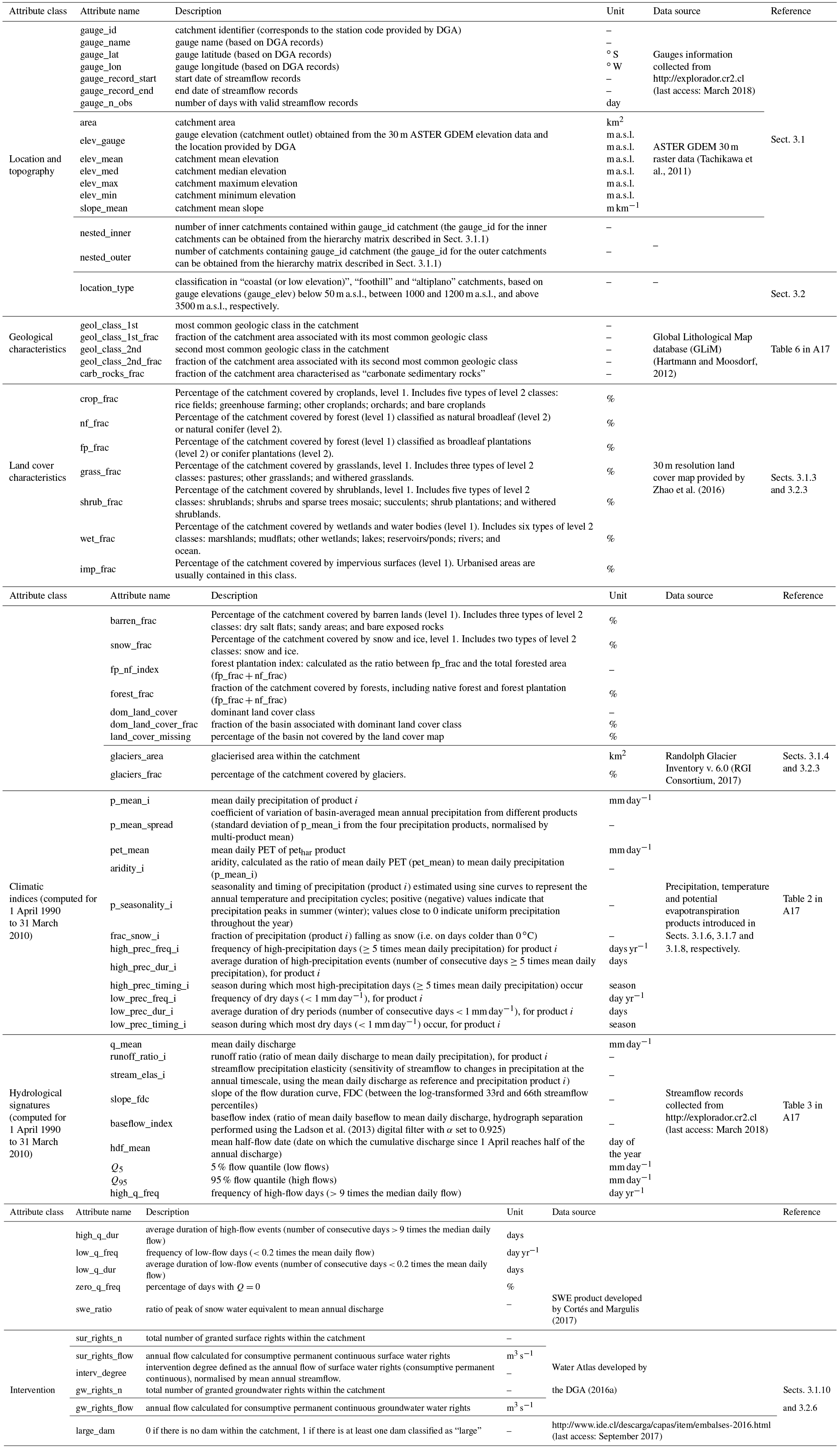
We introduce the first catchment dataset for large sample studies in Chile. This dataset includes 516 catchments; it covers particularly wide latitude (17.8 to 55.0∘ S) and elevation (0 to 6993 m a.s.l.) ranges, and it relies on multiple data sources (including ground data, remote-sensed products and reanalyses) to characterise the hydroclimatic conditions and landscape of a region where in situ measurements are scarce. For each catchment, the dataset provides boundaries, daily streamflow records and basin-averaged daily time series of precipitation (from one national and three global datasets), maximum, minimum and mean temperatures, potential evapotranspiration (PET; from two datasets), and snow water equivalent. We calculated hydro-climatological indices using these time series, and leveraged diverse data sources to extract topographic, geological and land cover features. Relying on publicly available reservoirs and water rights data for the country, we estimated the degree of anthropic intervention within the catchments. To facilitate the use of this dataset and promote common standards in large sample studies, we computed most catchment attributes introduced by Addor et al. (2017) in their Catchment Attributes and MEteorology for Large-sample Studies (CAMELS) dataset, and added several others.
We used the dataset presented here (named CAMELS-CL) to characterise regional variations in hydroclimatic conditions over Chile and to explore how basin behaviour is influenced by catchment attributes and water extractions. Further, CAMELS-CL enabled us to analyse biases and uncertainties in basin-wide precipitation and PET. The characterisation of catchment water balances revealed large discrepancies between precipitation products in arid regions and a systematic precipitation underestimation in headwater mountain catchments (high elevations and steep slopes) over humid regions. We evaluated PET products based on ground data and found a fairly good performance of both products in humid regions (r>0.91) and lower correlation (r<0.76) in hyper-arid regions. Further, the satellite-based PET showed a consistent overestimation of observation-based PET. Finally, we explored local anomalies in catchment response by analysing the relationship between hydrological signatures and an attribute characterising the level of anthropic interventions. We showed that larger anthropic interventions are correlated with lower than normal annual flows, runoff ratios, elasticity of runoff with respect to precipitation, and flashiness of runoff, especially in arid catchments.
CAMELS-CL provides unprecedented information on catchments in a region largely underrepresented in large sample studies. This effort is part of an international initiative to create multi-national large sample datasets freely available for the community. CAMELS-CL can be visualised from http://camels.cr2.cl and downloaded from https://doi.pangaea.de/10.1594/PANGAEA.894885.
- Article
(16967 KB) - Full-text XML
- BibTeX
- EndNote


Large sample hydrology has been recognised as a fundamental framework to advance hydrological science (e.g. Andréassian et al., 2006; Ehret et al., 2014). The insights provided by studying a large set of catchments complement the findings from intensive place-based studies, where more detailed analyses are conducted over a small number of catchments. A common approach in large sample studies is to explore interrelationships between catchment attributes describing landscape, climate and hydrologic behaviour, typically obtained from topography, soil types, geology, land cover and hydro-meteorological datasets (e.g. Oudin et al., 2008; Sawicz et al., 2011; Gupta et al., 2014; Newman et al., 2015; Addor et al., 2017). Accounting for catchment attributes in a comprehensive dataset serves various purposes. For example, comparative hydrology and catchment classification studies use these attributes to explore catchment (dis)similarities (e.g. McDonnell and Woods, 2004; Wagener et al., 2007; Sawicz et al., 2011; Berghuijs et al., 2014). Likewise, regionalisation studies incorporate catchment attributes to identify (hydro-climatically and physically) similar catchments that can be used to transfer model information from gauged to ungauged locations (Blöschl et al., 2013; Sawicz et al., 2011) – a fundamental motivation of the Predictions in Ungauged Basins (PUB) initiative (Sivapalan et al., 2003). In summary, the main goal of large sample applications is to learn from diversity in order to define generalizable rules that can help to improve the predictability of the water cycle. This is addressed by disentangling the interplay between landscape, climate and hydrologic behaviour, which provides insights into hydrological systems and into suitable model structures to represent them.
As highlighted by Gupta et al. (2014), a key challenge in large sample hydrology is data accessibility, which is particularly critical in data-scarce regions such as South America (see Fig. 2 in Gupta et al., 2014). Although there is a tendency for large sample datasets to be shared worldwide (see examples in Gupta et al., 2014), available hydro-meteorological records from different countries typically use different formats and come from different providers. Moreover, they are rarely spatially aggregated to the catchment scale, which makes it difficult for researchers and practitioners to use them for basin-oriented applications.
In this paper, we introduce a unique dataset that includes 516 catchments in Chile, and show how this dataset serves to improve our understanding of hydrological systems and their predictability through the assessment of (1) the uncertainties in two key meteorological variables (precipitation and PET) and (2) the impacts of anthropic intervention on catchment response.
The dataset built here consists of catchment boundaries in shapefile format, hydro-meteorological time series, and a suite of catchment attributes based on climate, hydrology, topography, geology, land cover, and water use. To facilitate and encourage the use of this dataset, and to promote common standards and formats in large sample studies, we compute five (out of six) classes of catchment attributes (location and topography, geology, land cover characteristics, climatic indices and hydrological signatures) used in Addor et al. (2017, referred to as A17 hereafter). A17 introduced the Catchment Attributes and MEteorology for Large-sample Studies dataset (CAMELS dataset), which encompasses meteorological and streamflow datasets collated by Newman et al. (2015) and provides quantitative estimates of a wide range of attributes for 671 catchments in the contiguous United States (CONUS). The CAMELS dataset has already been used in a myriad of applications, including assessment of streamflow skill elasticity to initial conditions and climate prediction (Wood et al., 2016), snow data assimilation for seasonal streamflow prediction (Huang et al., 2017), continental-scale hydrologic parameter estimation (Mizukami et al., 2017), and climate change impacts on the hydrology of the CONUS (Melsen et al., 2018), among others. Following this nomenclature, we name our dataset CAMELS-CL, which stands for CAMELS dataset in Chile. We add an attribute class not covered by A17: the degree of human intervention in each catchment. This novel information is valuable since anthropogenic activities may have major impacts on catchment behaviour, but human influence is often difficult to quantify, especially for hundreds of catchments.
We characterise hydrological systems in Chile by analysing the spatial distribution of catchment attributes provided in CAMELS-CL. Subsequently, we apply CAMELS-CL to assess uncertainties in precipitation and potential evapotranspiration estimates, and to quantify anthropic impacts on catchment response. To this end, we compared the different precipitation products and evaluated them based on the observed water balance. This analysis includes one national dataset (CR2MET) and three widely used global datasets (CHIRPS, MSWEP and TMPA); thus, the results may have implications beyond the domain covered by CAMELS-CL. Then, we assess PET products based on an independent set of PET point values calculated from meteorological records. Finally, we analyse human influence on catchment behaviour by relating hydrological signatures to a human intervention attribute calculated from water extraction information.
The paper is structured as follows: Sect. 2 describes the study area; Sect. 3 describes the collected datasets (Sect. 3.1) and provides a description of the derived catchment attributes with a discussion of their spatial distribution (Sect. 3.2); Sect. 4 presents the precipitation (Sect. 4.1) and potential evapotranspiration (Sect. 4.2) uncertainty analyses; Sect. 5 presents the analysis of human influence on catchment behaviour; and Sect. 6 summarises the main conclusions of the paper.
The area covered by CAMELS-CL corresponds to continental Chile, a territory with a distinct geographical configuration that spans 4300 km along a north–south axis over the west of South America (17.8∘ S to 55.0∘ S). The country lies on the Nazca and Antarctic tectonic plates. The tectonic activity in the Quaternary (early Pleistocene) led to the formation of the three main physiographic characteristics of the territory (from west to east): the coastal range, the intermediate depression, and the Andes Cordillera. Featuring altitudes well above 3000 m a.s.l., with summits up to 7000 m a.s.l. (e.g. Aconcagua mountain or Ojos del Salado volcano), the Andes act as an effective barrier for atmospheric flows, leading to particularly large precipitation amounts at high elevations (Garreaud, 2009) and to a noticeable contrast between the rainfall regimes of southern Chile (wet) and Argentinean Patagonia (dry).
Chile has 16 administrative regions (Fig. 1) split into four macro-zones defined by the Chilean Water Directorate (DGA), based on hydrological, climatic and topographic features (DGA, 2016a): North (from Arica and Parinacota to Coquimbo regions); Central (from Valparaiso to Maule regions); South (from Bio-Bio to Los Lagos regions); and Austral (from Aysén to Magallanes regions). To provide a more detailed description, we divided the North macro-zone into Far North (from Arica and Parinacota to Antofagasta regions) and Near North (from Atacama to Coquimbo regions), and the Austral macro-zone into the Austral Zone (Aysen region) and Southern Patagonia (Magallanes region). The resulting six macro-zones are presented in Fig. 1.
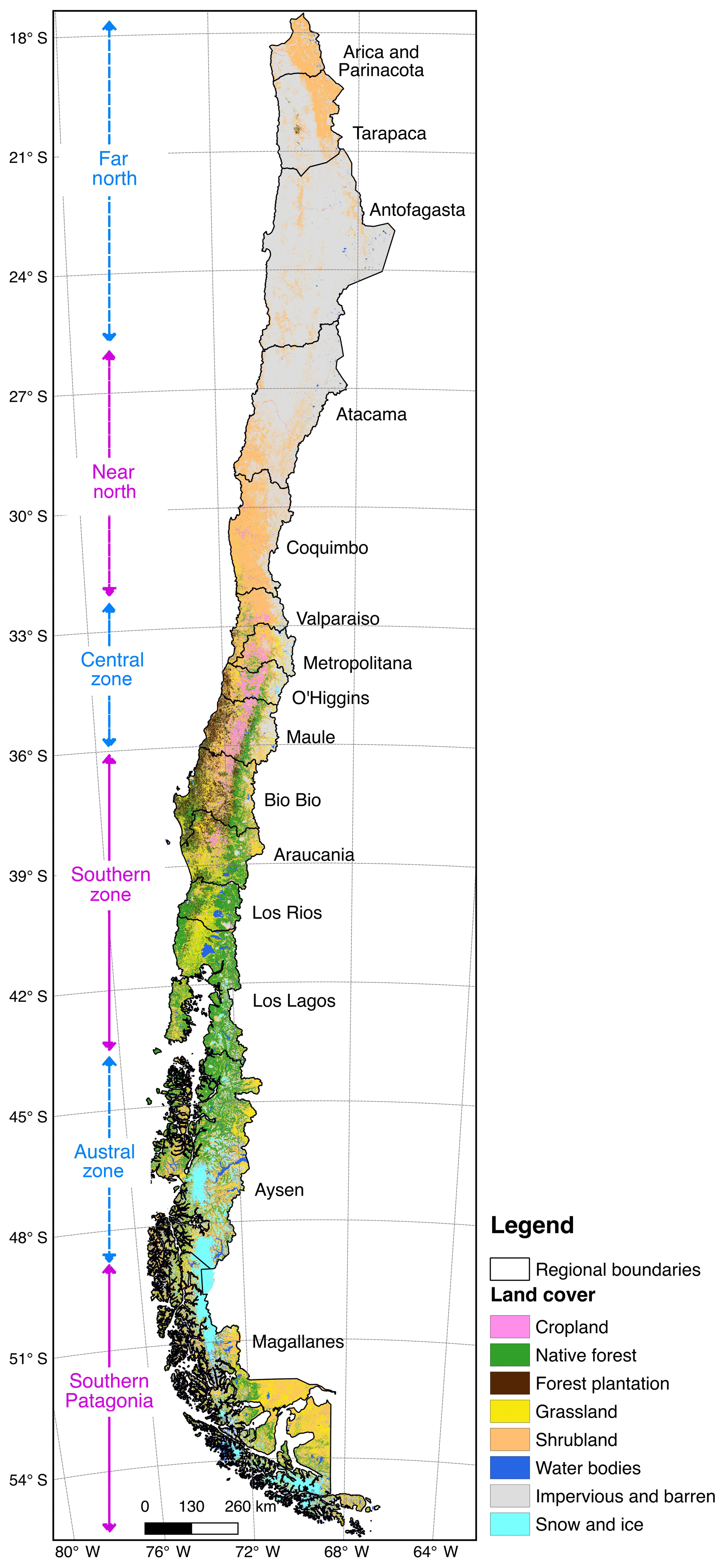
Figure 1Chilean regional boundaries and names, and the six defined macro-zones (blue and magenta arrows). The background colour corresponds to the main land cover classes, obtained from Zhao et al. (2016).
The country includes five primary climatic regimes according to the Köppen–Geiger climate classification (Kottek et al., 2006; Sarricolea et al., 2017). The Far North is dominated by a cold desert climate (BWk) and tundra (ET) along the Andes range. The Near North is characterised by a cold desert climate in the Atacama region and a cold semi-arid climate (BSk) in the Coquimbo region. The Central Zone is dominated by a sub-humid Mediterranean climate (Csb). The Southern Zone includes a humid Mediterranean climate in the Bio-Bio and Araucanía regions, and a temperate rain–oceanic climate (Cfb) in the Los Rios and Los Lagos regions. The Austral and Southern Patagonia zones are dominated by rain–cool oceanic (Cfc) and cold steppe (BSk) climates.
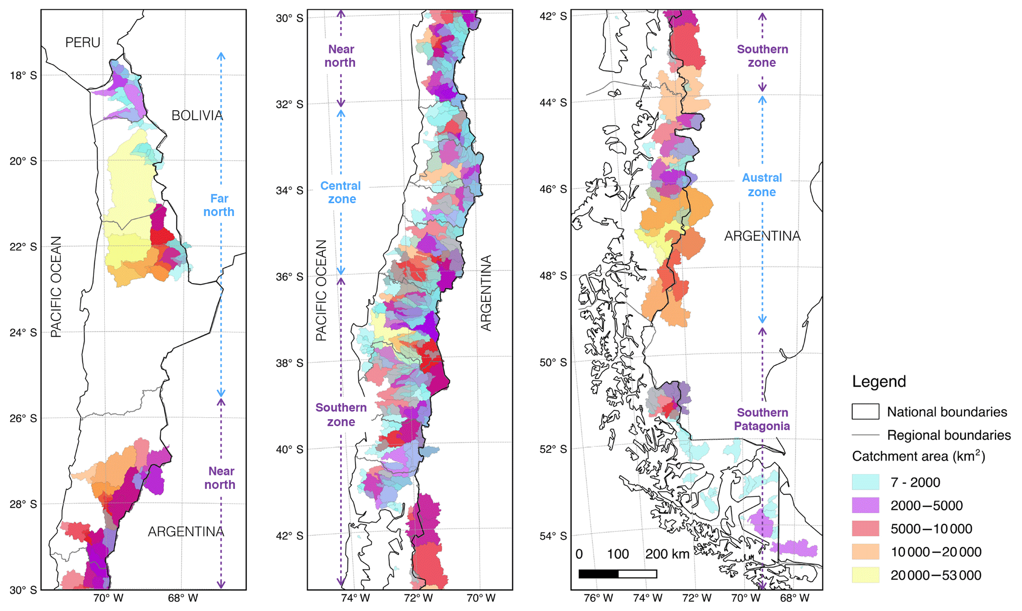
Figure 2Catchment boundaries and contributing areas (km2) of the 516 watersheds included in this study. The six defined macro-zones are indicated in blue and purple arrows.
3.1 Input data
3.1.1 Topography and catchment boundaries
The first step in the development of CAMELS-CL was the delimitation of catchment boundaries (Fig. 2). An official database for the Chilean hydrographic network was developed by the Instituto Geográfico Militar in 1984 (IGM, 1984) and updated by the DGA in 2014 (DGA and CIREN, 2014). This network delineation followed the Strahler hierarchy (Strahler, 1957), using the 30 m ASTER GDEM elevation data (Tachikawa et al., 2011). The DGA network includes 102 catchments, 491 sub-catchments and 1481 sub-sub-catchments, and has been largely used by government agencies, the private sector and the general public. However, a key limitation of this hydrographic network is that – given the methodology used for its implementation – the existing streamflow gauges do not correspond to catchment outlets. Furthermore, DGA catchment boundaries are truncated at the administrative national border, even though some catchments contribute runoff from the Bolivian and Argentinian territories. Since any hydrologic application within a controlled basin requires the total contributing area associated with streamflow measurements, and there is no official catchment boundary database, different studies have applied their own basin delineations, making it difficult to compare results.
To overcome this limitation, we created our own catchment boundary database for CAMELS-CL, defining the basin outlets at the location of 516 selected streamflow gauges (Sect. 3.1.5) and following only topographic-driven limits (not the administrative national border). A key challenge for this task is the mismatch between some station geographic coordinates reported by the DGA and the actual river network location – detected through the inspection of Google Earth imagery (Google, 2016). For some of those cases, expert advice was obtained from DGA technicians regarding gauge locations, while, for others, ancillary information (e.g. gauge name, road maps, Google Earth imagery) was used to determine the most likely location.
Basin delineation was performed in Quantum GIS (QGIS Development Team, 2015) by using watershed delineation packages from the Geographic Resources Analysis Support System (GRASS) (Neteler et al., 2012) and 30 m ASTER GDEM as input elevation data. Given the location of streamflow gauges, several catchments collected in this dataset are nested. We report this by using a logical hierarchy matrix indicating which basins are contained within another catchment of the dataset. The hierarchy matrix can be used to filter independent catchments, which is required for some applications such as hydrological modelling of large basins, catchment classification and parameter regionalisation.
The main topographic properties, including area, median, mean, minimum and maximum elevation, and mean slope, were computed for each catchment from ASTER GDEM 30 m raster data, clipped by the catchment boundary polygons and processed with the R raster package (Hijmans, 2016). An important limitation of this dataset is that its spatial resolution is relatively coarse, which can lead to errors when delineating catchments over very flat regions (such as the Far North; see Sect. 3.2.1).
3.1.2 Geology
Catchment-scale geological characteristics were retrieved from the Global Lithological Map database (GLiM) produced by Hartmann and Moosdorf (2012). GLiM is a compilation of national datasets into a unified global map. In the case of Chile, GLiM uses the map produced by the Servicio Nacional de Geología y Minería (Sernageomin, 2004), which has a resolution of 1:1 000 000 and is the most complete and commonly used map for the country. For each catchment, we reported the most and second-most frequent geological classes, as well as the fraction of the catchment they cover. We also extracted the fraction of the catchment described as “carbonate sedimentary rocks”, as it is a useful indicator of the presence of karstic systems.
3.1.3 Land cover
We used the 30 m resolution land cover map provided by Zhao et al. (2016), which integrates multi-seasonal Landsat 8 imagery acquired during 2013 and 2014, complemented with Moderate Resolution Imaging Spectroradiometer (MODIS) Enhanced Vegetation Index data, and high-resolution imagery on Google Earth. The classification scheme adopted by Zhao et al. (2016) was designed with Chilean geographers and biodiversity researchers, based on the FROM-GLC project (Gong et al., 2013), which is similar to the Land Cover Classification System (Di Gregorio and Jansen, 2005). This classification scheme is compatible with other land cover classification systems such as FAO or IGBP, with minor ancillary data. It consists of 10 main (level 1) classes (Fig. 1): croplands; forests, grasslands; shrublands; wetlands; water bodies; impervious surfaces; barren lands; and snow and ice. Some classes were refined in level 2 (e.g. forests were separated into native forest and exotic forest plantation) and level 3 subclasses (a total of 30 and 35 subclasses, respectively). For CAMELS-CL, we used the R raster package (Hijmans, 2016) to clip the land cover map within each catchment boundary polygon, and compute the fractional area associated with each class or subclass (as described in Table 3).
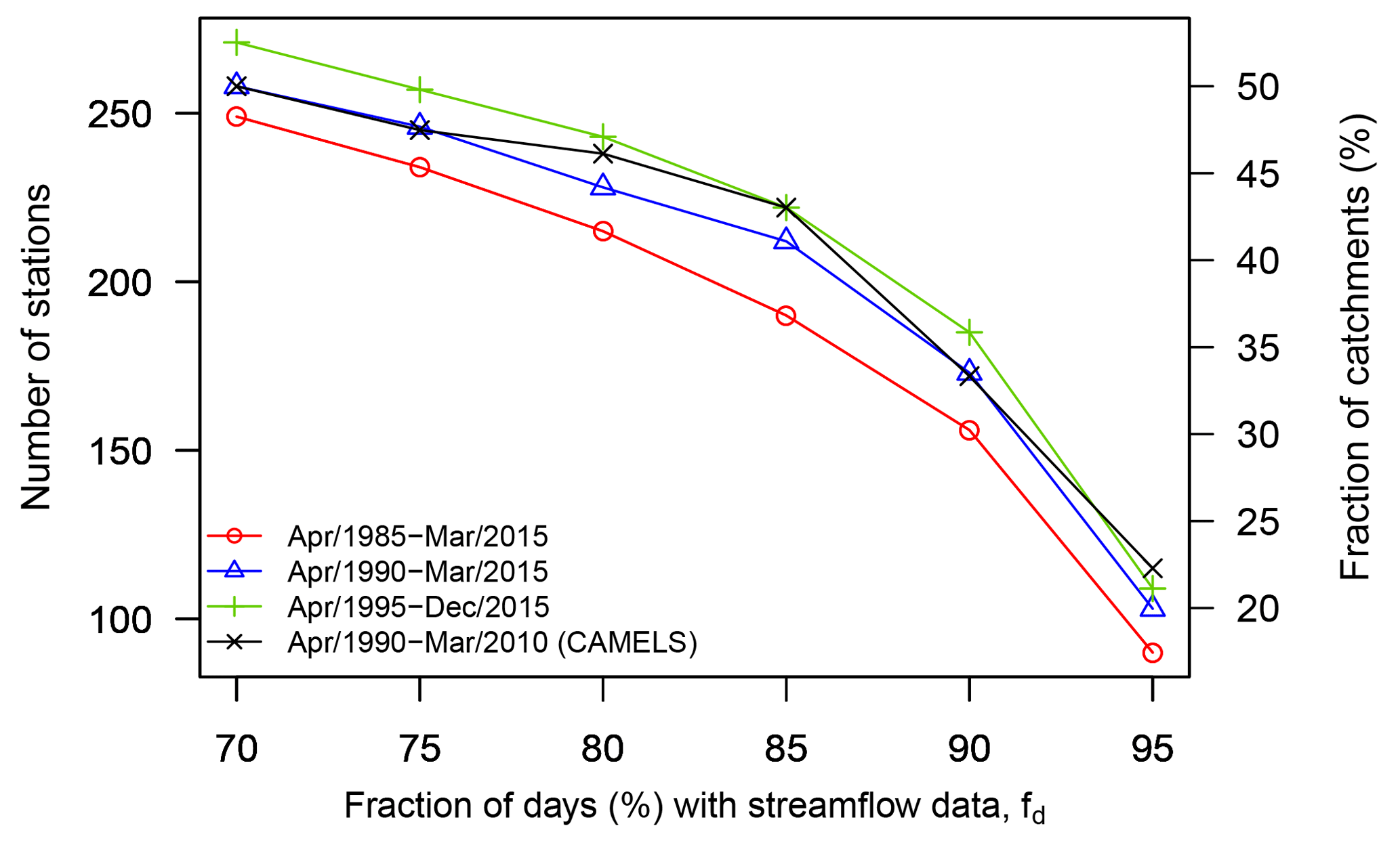
Figure 3Number of stations (left y axis) with at least fd % of days with daily streamflow records, for different periods. The right y axis shows the percentage of catchments (out of 516) that meets the criterion. The period used in the CAMELS dataset (Addor et al., 2017) was included as a reference.
3.1.4 Glaciers
Glaciers in Chile can be found at several locations, varying from small ice bodies at high-elevation sites in the Atacama region to alpine glaciers in the Central Zone and the large Patagonian ice fields in the Austral and Southern Patagonia regions (Pellicciotti et al., 2014). Even though the land cover map from Zhao et al. (2016) identifies areas of snow and ice, we included a global glacier inventory for calculating the degree of glacierisation of the selected catchments. Glacier inventories have the advantages of using geomorphologic glacier-delineation techniques and the recognition of debris-covered areas that cannot be identified by land cover classification schemes. In this study, we used the latest version of the Randolph Glacier Inventory (RGI 6.0; RGI Consortium, 2017). RGI 6.0 is a globally complete inventory of glacier outlines, and it is widely used in regional and global studies on land surface fluxes, climatology and meteorology (e.g. Huss and Hock, 2015; Marzeion et al., 2012; Mernild et al., 2017). We preferred to use RGI 6.0 rather than the Chilean glacier inventory from the DGA (DGA, 2014) because there are portions of some catchments lying in Argentinean territory (Fig. 2). RGI 6.0 was clipped within each catchment and two attributes were computed: the total glacierised area (km2) and the percentage of glacierised area in the catchment (%).
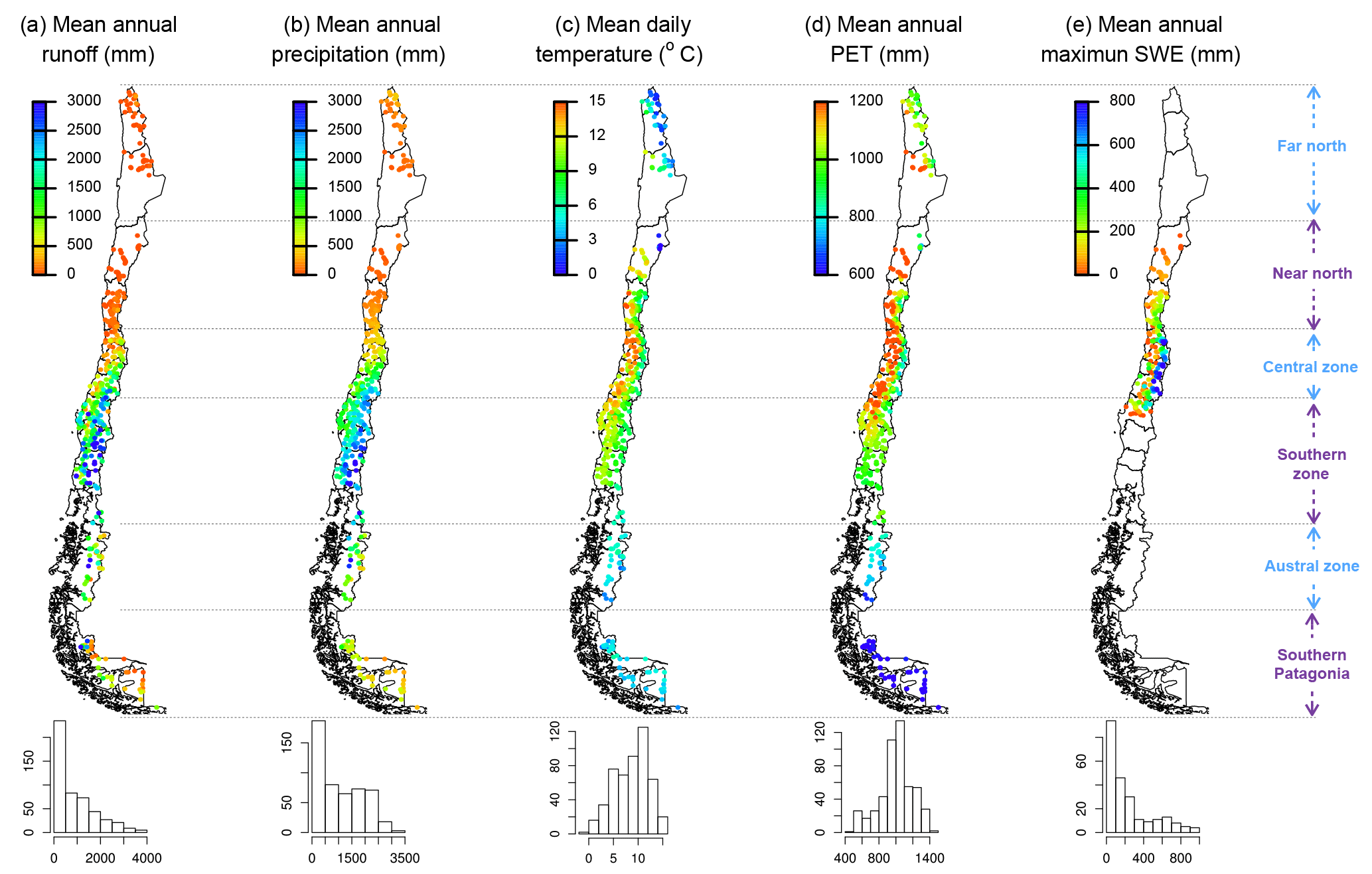
Figure 4Mean annual hydro-meteorological variables, calculated for the complete recording period of each variable. (b) and (d) were generated with precipcr2met and pethar products, respectively. The SWE product in (e) covers only the Near North and Central zones. The histograms indicate the number of catchments (out of 516) in each bin. The points represent the locations of catchment outlets.
3.1.5 Streamflow
We compiled daily streamflow records for gauges maintained by the DGA, available from the CR2 Climate Explorer (http://explorador.cr2.cl/, last access: March 2018). From the 809 gauges included there, we selected those currently operational (independently of their data period) or suspended after 31 December 1980 with a record period longer than 10 years. We also discarded gauges located in artificial channels, ending up with 516 selected gauges. The record lengths from the selected gauges range from 192 to 366 667 days, with a mean (median) of 10 979 (9909) days. Figure 3 illustrates the availability of daily streamflow records for different time periods (represented by different colours), which is mainly due to the different record periods of the selected gauges. Further, sparse missing daily records may be found in streamflow time series due to specific extreme events, where the station might have not worked properly or might have been broken. Note that hydrological year is considered from 1 April to 31 March. As expected, the number of stations decreases with longer data availability. For example, if only stations with at most 5 % of missing data were selected, this would lead to a subset of 90 to 115 stations (which corresponds to 18 % and 22 % of the total number of catchments within the database, respectively), depending on the time period selected. When considering all stations with at most 30 % of missing data, then 249 to 258 stations (48 % and 50 % of catchments, respectively) would meet this criterion, depending on the period (Fig. 3). Figure 4a presents the mean annual discharge for each station (computed for the entire record period).
3.1.6 Precipitation
In most cases, precipitation is the main driver of hydrological systems. However, the geographical distribution of this variable is highly uncertain, even in densely monitored regions (Tian and Peters-Lidard, 2010; Woldemeskel et al., 2013). This limitation is aggravated in regions with difficult accessibility, where only a sparse network of meteorological stations is available. In order to account for robust precipitation estimates and to characterise the uncertainty of this variable, we processed catchment-scale precipitation from four different products, whose main characteristics are summarised in Table 1. Daily precipitation fields provided by each product were clipped and averaged within the catchment boundaries, resulting in four daily time series for each catchment, named precipcr2met, precipchirps, precipmswep and preciptmpa.
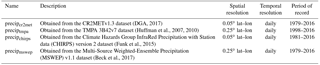
The precipcr2met time series was derived from CR2MET, a spatially distributed daily precipitation product developed for Chile, which is currently used by DGA to update the national water balance (DGA, 2017). The CR2MET product is partly based on a statistical downscaling of ERA-Interim reanalysis data (Balsamo et al., 2015). The method builds on multiple linear regression models used to transfer precipitation, moisture fluxes and other variables from ERA-Interim onto 0.05∘ resolution precipitation estimates. The statistical models, which also consider a number of topographic parameters, were calibrated using a large network of quality-controlled rain-gauge records. Depending on the distance of a given grid cell to neighbouring stations, the final product was obtained from merging downscaled precipitation and spatially interpolated in situ observations. Further information about formulation, quality control and product assessments can be found in DGA (2017).
The three satellite-based precipitation products used in CAMELS-CL were selected following the inter-comparison reported by Zambrano-Bigiarini et al. (2017) for the entire Chilean territory. The precipchirps time series was computed from the Climate Hazards Group InfraRed Precipitation with Station data version 2 (CHIRPS, Funk et al., 2015), a long-term (1981 to near present), quasi global (50∘ N to 50∘ S) daily dataset available at a spatial resolution of 0.05∘, designed to monitor agricultural drought and global environmental changes over land. CHIRPS uses the Tropical Rainfall Measuring Mission Multi-Satellite Precipitation Analysis version 7 (TRMM 3B42v7) in order to calibrate global cold cloud duration rainfall estimates (Funk et al., 2015). CHIRPS also incorporates surface rain-gauge data in order to reduce estimation biases, based on public and private monthly data. Originally, this dataset spanned from 50∘ N to 50∘ S, but since November 2012 data have not been produced south of 46∘ S. More information can be found in Funk et al. (2015).
Variable precipmswep was computed from Multi-Source Weighted-Ensemble Precipitation (MSWEP, Beck et al., 2017) data version 1.1, a fully global precipitation dataset released in June 2016, with 3-hourly temporal and 0.25∘ spatial resolutions, specifically produced for hydrological modelling applications. MSWEP was designed to improve the performance of satellite products in representing precipitation over mountainous, tropical, and snowmelt-driven regions. The algorithm used in MSWEP merges observed rain-gauge data, satellite observations and reanalysis data to provide reliable precipitation estimates over the entire globe. In this paper, we used daily data from MSWEP version 1.1, but newer versions (already available) will be included in CAMELS-CL after validation with ground measurements in Chile.
Finally, preciptmpa was computed from the Tropical Rainfall Measuring Mission (Huffman et al., 2007) Multi-satellite Precipitation Analysis (TMPA) dataset, which provides quasi global (50∘ N to 50∘ S) precipitation estimates at 0.25∘ spatial resolution. TMPA integrates infrared and passive microwave data from a wide variety of satellite-borne precipitation-related sensors. In this study, we used TRMM research product 3B42v7, which makes use of Global Precipitation Climatology Project (GPCP; Adler et al., 2003) and Climate Assessment and Monitoring System (CAMS, Ropelewski et al., 1984) data to rescale its estimations on a monthly basis.
3.1.7 Temperature
Daily time series of minimum, maximum and mean temperatures for each catchment were also derived from the CR2MET dataset (DGA, 2017). Daily minimum and maximum temperatures in CR2MET (CR2MET/Tmax and CR2MET/Tmin, respectively) were mapped for the period 1979–2016 using a slightly different approach than the one used for precipitation (Sect. 3.1.6). In this case, the method used land surface temperature (LST) estimates from MODIS satellite retrievals, in addition to near-surface temperature provided by ERA-Interim. Multivariate regression models for both CR2MET/Tmax and CR2MET/Tmin were developed using LST as part of the explanatory variables and local temperature records in Chile as target data. Given the data gaps and relatively short period available for LST, the final product was derived for the whole period (1979–2016) by fitting the ERA-Interim data to the preliminary (incomplete) MODIS-based product. To get mean daily temperatures (CR2MET/Tmean), the long-term CR2MET/Tmax and CR2MET/Tmin were used to adjust the ERA-Interim 3-hourly near-surface temperature. The adjusted 3-hourly data were then averaged to derive CR2MET/Tmean. Gridded daily mean, minimum and maximum temperatures from CR2MET (0.05∘ lat–lon resolution) were clipped to obtain basin-averaged daily time series for CAMELS-CL, named Tmean, Tmin and Tmax, respectively.
3.1.8 Potential evapotranspiration
We processed catchment-scale PET from two different sources. The first PET product uses the formulae proposed by Hargreaves and Samani (1985), which is solely based on surface temperature data (see Hargreaves and Allen, 2003, for further details). We used CR2MET/Tmax and CR2MET/Tmin (described in Sect. 3.1.7) to generate a gridded PET estimate (PEThar).
The second PET data included in CAMELS-CL (PETmod) are those provided by the MODIS PET product (MOD16 collection 5; Mu et al., 2005), which is processed from different sources of information, including leaf area index and fractional photosynthetically active radiation, FPAR/LAI (MOD15A2; Myneni et al., 2002), land cover type 2 (MOD12Q1; Friedl et al., 2002), albedo (MCD43B2 and MCD43B3; Jin et al., 2003; Lucht et al., 2000), and daily meteorological reanalysis data from NASA's MERRA GMAO (GEOS-5). MOD16 is calculated following the Penman–Monteith approach (Howell and Evett, 2001), and the final product is available at an 8-day temporal resolution for the period 2000–2014, on a 1×1 km2 grid. As for other gridded variables, the PEThar and PETmod products were clipped and averaged within basin boundaries to generate daily (called pethar) and 8-day (called petmod) catchment-scale time series, respectively.
3.1.9 Snow water equivalent
We processed daily snow water equivalent (SWE) data using the 180 m resolution SWE product generated by Cortés and Margulis (2017), which covers the Near North and Central zones (25–37∘ S). Cortés and Margulis (2017) obtained SWE ensemble estimates from forward modelling “prior” values, which were conditioned through the assimilation of historical fractional snow-covered area (fSCA) data from Landsat TM, ETM+ and OLI sensors. The “posterior” SWE and fSCA estimates were probabilistically conditioned on the observed depletion record from Landsat, the uncertainty in fSCA observations, and the forward model state uncertainty. The fSCA retrieval was obtained with a spectral un-mixing algorithm (Cortés et al., 2014). The forward models for prior ensemble generation were the SSiB3 land surface model (Yang et al., 1997) and a snow depletion curve model (SDC; Liston, 2004). Detailed assessments of this reanalysis framework were performed for the Sierra Nevada using in situ sensor data (Margulis et al., 2016) and for the Andes (Cortés et al., 2016) using snow survey points, site years of peak annual snow pillow and snow course SWE observations. Validation results showed unbiased posterior SWE estimates with a correlation coefficient of 0.73, an RMSE of 0.29 m and a mean error of less than 0.01 m using snow pillow and snow course peak SWE. Results using snow survey data showed similar unbiased estimates, with a correlation coefficient of 0.50, an RMSE of 0.29 m and a mean error of less than 0.01 m. The daily SWE gridded product generated by Cortés and Margulis (2017) was clipped and averaged within the catchment boundaries to obtain daily time series for each catchment.
3.1.10 Water rights and reservoir information
A public reservoir dataset (http://www.ide.cl/descarga/capas/item/embalses-2016.html, last access: September 2017) was processed to identify the presence of dams within catchments. We also compiled and processed granted water rights available from the National Water Atlas (DGA, 2016a). This water allocation dataset includes information about the source (surface or groundwater), the type of right (i.e. consumptive or non-consumptive), use (i.e. industrial, irrigation, domestic and drinking water, hydroelectric power, pisciculture, mining, and classified as “other uses”), annual allocated flow (expressed in units of volume per time or as “shares”), and temporal allocation (i.e. permanent and continuous, permanent and discontinuous, permanent and alternated, eventual and continuous, eventual and discontinuous, or eventual and alternated). A detailed explanation of this water right classification can be found in Carey (2014). A key limitation of this dataset is the lack of information on the actual use of granted rights (Larraín, 2006). Additionally, some water right records have incomplete information (e.g. missing coordinates, water volume assigned and temporal allocation).
Figure 5 illustrates water allocation in central–southern Chile (30–43∘ S), showing surface and groundwater rights (all types). It is clear that groundwater rights dominate in central Chile (31–36∘ S), especially in low-elevation areas, compared to surface water rights. On the other hand, more surface water rights are granted in southern Chile, especially within high-elevation areas towards the Andes.
3.2 Derived catchment attributes
We computed 70 catchment attributes grouped into six classes (Table 2). To motivate the use of common standards in the development of large sample catchment datasets, we included most of the attributes presented by A17. A comparative summary between CAMELS and CAMELS-CL attributes is presented in Table 2, from which one can note that the attributes from classes climatic indices and hydrological signatures were fully adopted from A17. The attributes from the class soil characteristics were not computed at this stage since there is no publicly available national dataset. Given the differences in input datasets, some of the attributes from the classes location and topography, geologic characteristics, and land cover characteristics in A17 were not computed here. On the other hand, new attributes were derived for the classes' location and topography (Sect. 3.2.1), land cover characteristics (Sect. 3.2.3) and hydrological signatures (Sect. 3.2.5). Further, a new class was added to describe the degree of intervention within the catchments (Sect. 3.2.6).
Table 2Summary of attributes computed in CAMELS and CAMELS-CL.
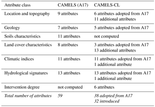
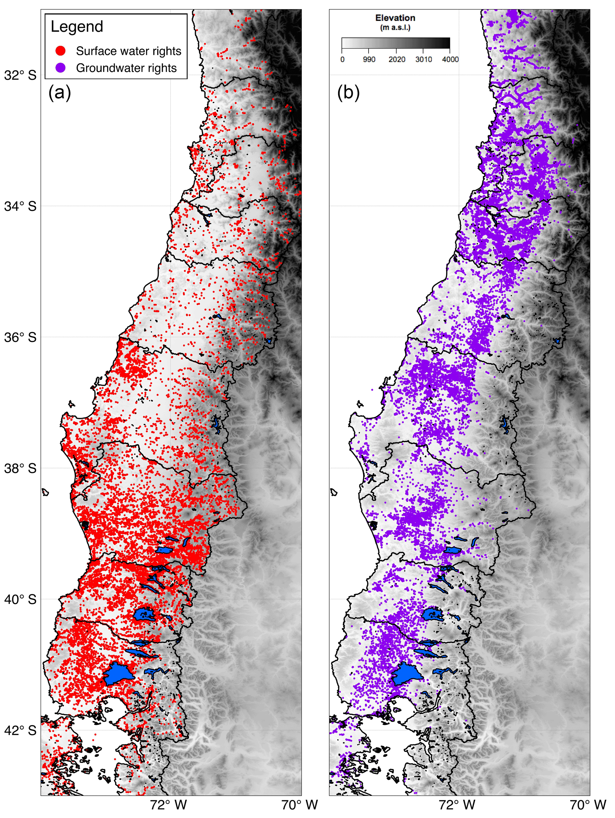
Figure 5Surface (a) and ground (b) water rights (consumptive, non-consumptive, permanent, eventual and alternated) granted by the Chilean Water Directorate (DGA) for a portion of the country. Background colours represent topography (greyscale) and the main water bodies (highlighted in blue).
A complete list of catchment attributes included in CAMELS-CL, their description and the corresponding data sources are presented in Table 3. To ensure the reproducibility of our results, the reference to the explicit formulation of climatic indices and hydrological signatures is provided in Table 3. Discussions on the spatial distribution of catchment attributes, separated by class, are presented in the following sub-sections.
3.2.1 Location and topography
Figure 6 shows 6 (out of 14) location and topography attributes. Figure 6a presents the elevation of catchment outlets, illustrating two main elevation gradients: (i) a north to south (N–S) decrease, starting with high-elevation basins in the Far North macro-zone – which corresponds to the southern portion of the Altiplano Plateau (18–22∘ S) (Allmendinger et al., 1997) – towards lower elevations in the southern macro-zones; and (ii) an east to west (E–W) gradient, dominated by high elevations in the Andes (located along the eastern border) decreasing towards sea level at the western border. This gauge elevation attribute can be used to classify catchments based on their location with respect to the coast or the Andes. We proposed the attribute location_type (see Table 3 and Fig. 6f) with three categories: coastal (or low elevation), foothills, and Altiplano catchments, defined by gauge elevations lower than 50 m a.s.l., between 1000 and 1200 m a.s.l., and above 3500 m a.s.l., respectively.
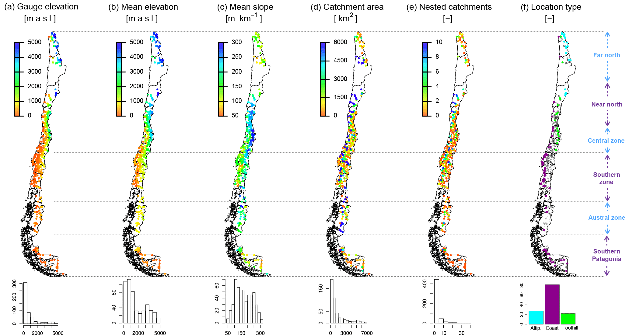
Figure 6Location and topography. For visualisation purposes, catchment areas (d) are shown up to their 90th percentile. The histograms indicate the number of catchments (out of 516) in each bin.
Figure 6b reveals smoother N–S and E–W gradients of basin-averaged elevations, compared to gauge elevation gradients (Fig. 6a). This is because the mean elevation calculated for downstream catchments includes nested catchments (located at higher altitudes). From the complete set of catchments, 178 have a mean elevation greater than 2000 m a.s.l. The spatial distribution of mean catchment slopes follows different patterns depending on the macro-zone (Fig. 6c). The Far North – dominated by the flat Altiplano Plateau – exhibits relatively small variations in mean slopes, with relatively low values. From the Near North to Austral zones, the mean slope shows a spatial distribution similar to that from mean elevation, with an E–W gradient dominated by high slopes in the Andes and flatter areas towards the sea. In Southern Patagonia, such an E–W gradient is reversed given the relative position of the Andes.
The spatial distribution of basin areas shows a general increase from east to west (Fig. 6d), which is consistent with smaller headwater catchments at the Andes and larger downstream catchments towards the sea. Some exceptions to this E–W distribution pattern are catchments located near the eastern border, featuring either a N–S drainage direction or a portion of their total contributing area in Argentina (beyond the eastern national border). Additional exceptions to such E–W distribution are small inner sub-catchments near the western border or small headwater catchments originated at the Chilean Coastal Range, which runs from north to south along the Pacific coast and reaches up to 3000 m a.s.l. in the Antofagasta region (Figueroa and Moffat, 2000).
Given that all catchments were delineated using available streamflow gauge locations as outlets (Sect. 3.1.1), the contributing area (Fig. 6d) is not necessarily correlated with the number of nested basins within each catchment (Fig. 6e). For example, some small catchments might be highly instrumented (i.e. with many controlled nested basins, because of – for example – water allocation priorities or having a high population density like those in Region Metropolitana, which concentrates more than 40 % of the country's population), while large but poorly instrumented catchments might not have inner basins defined.
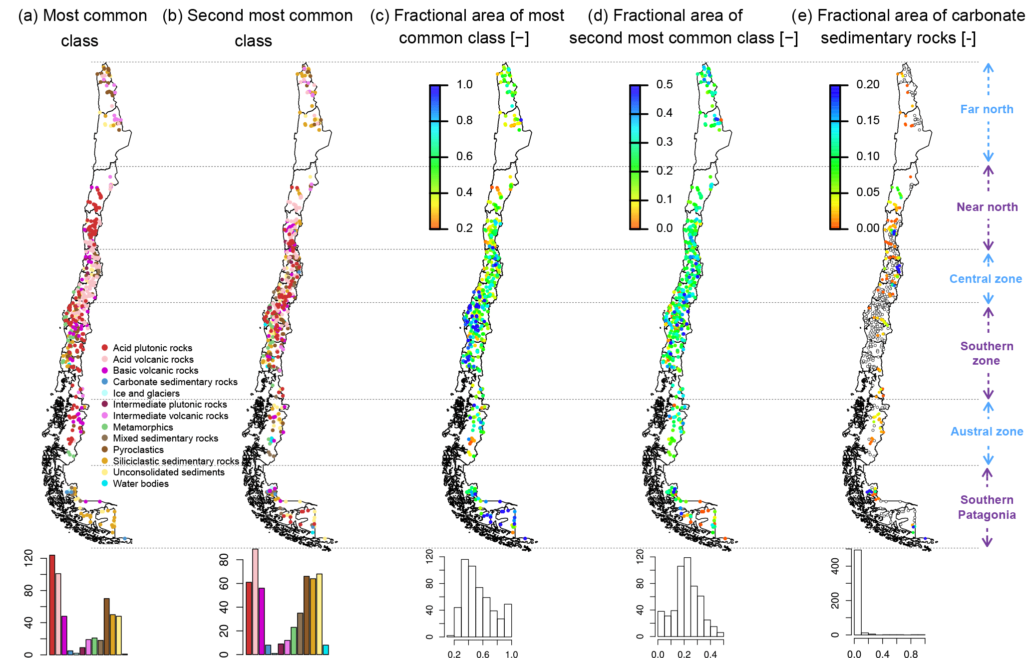
Figure 7Geology attributes. The histograms indicate the number of catchments (out of 516) in each bin.
3.2.2 Geological attributes
Overall, the most common dominant geological classes within CAMELS-CL catchments are acid plutonic rocks (24 %), acid volcanic rocks (20 %) and pyroclastic (14 %). In the Far North zone, there is a strong presence of Pyroclastics, Siliclastic sedimentary rocks and Intermediate volcanic rocks (Fig. 7a and b), which can result in the connection of groundwater systems through fractured volcanic rocks (DGA, 1986). This means that there might be differences between surface catchment boundaries (based on topography) and the extension of groundwater systems, which should be considered when analysing basin-scale hydrological response. Figure 7a also indicates that strong geological differences may exist between neighbouring catchments. Furthermore, one can see generally high geological variability within the catchments. Indeed, the dominant geological class covers less than half of the contributing area in most catchments, as indicated by the histogram in Fig. 7c. The presence of carbonate sedimentary rocks is particularly low (Fig. 7e), with only 24 catchments having at least 10 % of this type of rock. This suggests low formation of karst, a subsurface characteristic featuring large fissures and voids, which results in fast infiltration rates and preferential permeability channels (La Moreaux et al., 1984).
3.2.3 Land cover attributes
As summarised in Table 2, five land cover attributes in A17 were not computed since the land cover map used here (from Zhao et al., 2016) does not provide information about leaf area index, green vegetation fraction, or depth. Instead, we included land cover attributes based on the catchment area encompassed by the main classes of the land cover dataset (Table 3). The first nine land cover attributes described in Table 3 were computed as the percentage of the catchment area covered by level 1 and 2 land cover classes defined by Zhao et al. (2016). We also computed a forest plantation index to quantify the ratio between forest exotic plantation (mainly Pinus radiata and Eucalyptus spp.) and native forest within a catchment, which is critical information for forest hydrology and ecosystem studies (e.g. Lara et al., 2009).
Considering that several catchments (almost 50; Fig. 1) extend beyond the Chilean territory, a key limitation of the land cover attributes derived from Zhao et al. (2016) is the lack of information outside the national boundary. To address this, we generated an attribute indicating the fractional catchment area contained within the land cover map, serving also as a quality flag for basin-averaged land cover characteristics.
Another limitation of the land cover map and derived attributes is that there is no characterisation of inter-annual variability (the map was constructed by using imagery from 2013 and 2014). This can be particularly important for land cover types that are sensitive to climatic variations, such as altiplanic wetlands, which largely influence the hydrology in the Far North. This limitation is also critical for classes featuring drastic changes within time, such as forest plantation and cropland.

Figure 8Land cover characteristics. Values below the colour bar lower limits are shown in blank (i.e. blank points in panel a represent no forest cover, and in e they represent no missing land cover data within those catchments). The histograms indicate the number of catchments (out of 516) in each bin.
Figure 8 illustrates a subset of the land cover attributes listed in Table 3. Figure 8a shows the forested (native forests and forest plantation types) catchment area, which prevails in the Southern Zone, Austral Zone and Southern Patagonia. In forested catchments, exotic forest plantations dominate the coastal areas of the Central and Southern zones, with forest plantation indices up to 1 (Fig. 8b). Such a distribution illustrates the extensive land use change experienced in southern–central Chile over the last 50 years, where native forests have been progressively converted into agricultural lands and forest plantations (Armesto et al., 2010; Miranda et al., 2015). This conversion has had significant impacts on forest ecosystem services such as water provision (Jones et al., 2017; Lara et al., 2009).
Figure 8c and d show that the Far and Near North zones have more homogeneous land cover types, with shrublands and impervious lands occupying more than 60 % of the catchment areas. In southern areas, the coverage of the dominant classes decreases substantially, transitioning towards a mosaic of different land cover types. Missing land cover data are presented in Fig. 8e, which should be accounted for if the land cover attributes of the affected catchments (i.e. the ones with portions in Argentina, as shown in Fig. 2) are used for applications such as catchment classification or parameter regionalisation.
Because of the glaciological contributions to the water balance within the domain (Mernild et al., 2017; Le Quesne et al., 2009), we added two attributes (Table 3) based on information from the glacier inventory described in Sect. 3.1.4. We found that 255 catchments (48 % of the total) have some degree of glacierisation, reaching up to 62 % in the Geike River catchment in Southern Patagonia. The catchments with the largest degree of glacierisation (more than 15 %) are located in the Austral and Southern Patagonia regions, followed by the Olivares and Volcan river catchments (about 14 %) in the Central Zone. The glaciers included in CAMELS-CL span 7321 km2, corresponding to almost a quarter of the glacierised area in the southern Andes (RGI Consortium, 2017).
3.2.4 Climatic indices
To allow direct comparisons between CAMELS (A17) and CAMELS-CL, climatic indices were computed for the same period as in A17, i.e. water years 1990 to 2009, corresponding to 1 April 1990 to 31 March 2010 for Chile. If these indices are required for different periods, the formulae provided in the references from Table 3 can be used with the raw hydro-meteorological time series (available from the CAMELS-CL website). The complete spatial and temporal coverages of meteorological variables allow the estimation of climatic indices for all 516 catchments – in contrast to hydrological signatures, computed for a subset of catchments (Sect. 3.2.5). Precipitation and PET-based attributes were calculated for all precipitation products (Sect. 3.1.6) using the daily PET product (pethar, Sect. 3.1.8).
Table 3Summary of catchment attributes. Climate indices and hydrological signatures were computed for the period 1 January 1990–31 December 2010. Index i refers to the precipitation product (i=1, 2, 3, 4 for precipcr2met, preciptmpa, precipchirps and precipmswep, respectively).
The climatic attributes presented in Figs. 4 and 9 reveal basic features of Chilean climatology, described in more detail by Miller (1976) and Garreaud et al. (2017), among others. Mean annual precipitation ranges from less than 10 mm yr−1 in the Atacama Desert (northern Chile) to more than 3000 mm yr−1 in western Patagonia (Fig. 4b). Such a marked precipitation gradient reflects the relative influence of the subtropical, semi-permanent south-eastern Pacific anticyclone, and the frequent incursion of frontal systems at higher latitudes. The frequency of high-precipitation events also increases southward, with a maximum in southern–central Chile (Fig. 9d). The Andean domain in the Far North (Chilean Altiplano), receiving about 300 mm yr−1 above 4000 m a.s.l., is influenced by the monsoonal regime developing over the interior of the continent. In addition to the N–S gradient, precipitation increases strongly in the west–east direction due to the orographic enhancement of air masses over the windward slope of the Andes Cordillera (a factor of 2–3 between lowlands and windward slopes; Viale and Garreaud, 2014). PET has a more restricted range than precipitation (400–1400 mm yr−1; Fig. 4d); therefore, the aridity index (PET/P, Fig. 9c) is higher in northern Chile (>1.0) compared to that of southern regions (<1.0). A positive precipitation seasonality (Fig. 9a) in northern Chile indicates precipitation peaks during summer (DJF), following the monsoonal precipitation regime governing in this region (Fig. 9f). In contrast, the negative seasonality values obtained for all macro-zones, except the Far North and Southern Patagonia, illustrate the increased storm frequency and high-precipitation events in most of the country during the winter (JJA) (Fig. 9a). Seasonality values close to zero indicate uniform precipitation throughout the year in Southern Patagonia (Fig. 9a and f). The zero-temperature isotherm during winter storms ranges between 1500 and 4000 m a.s.l., so most of the precipitation is liquid along the coast and interior valleys (Fig. 9b), while a larger fraction of solid precipitation is obtained in high-elevation basins.
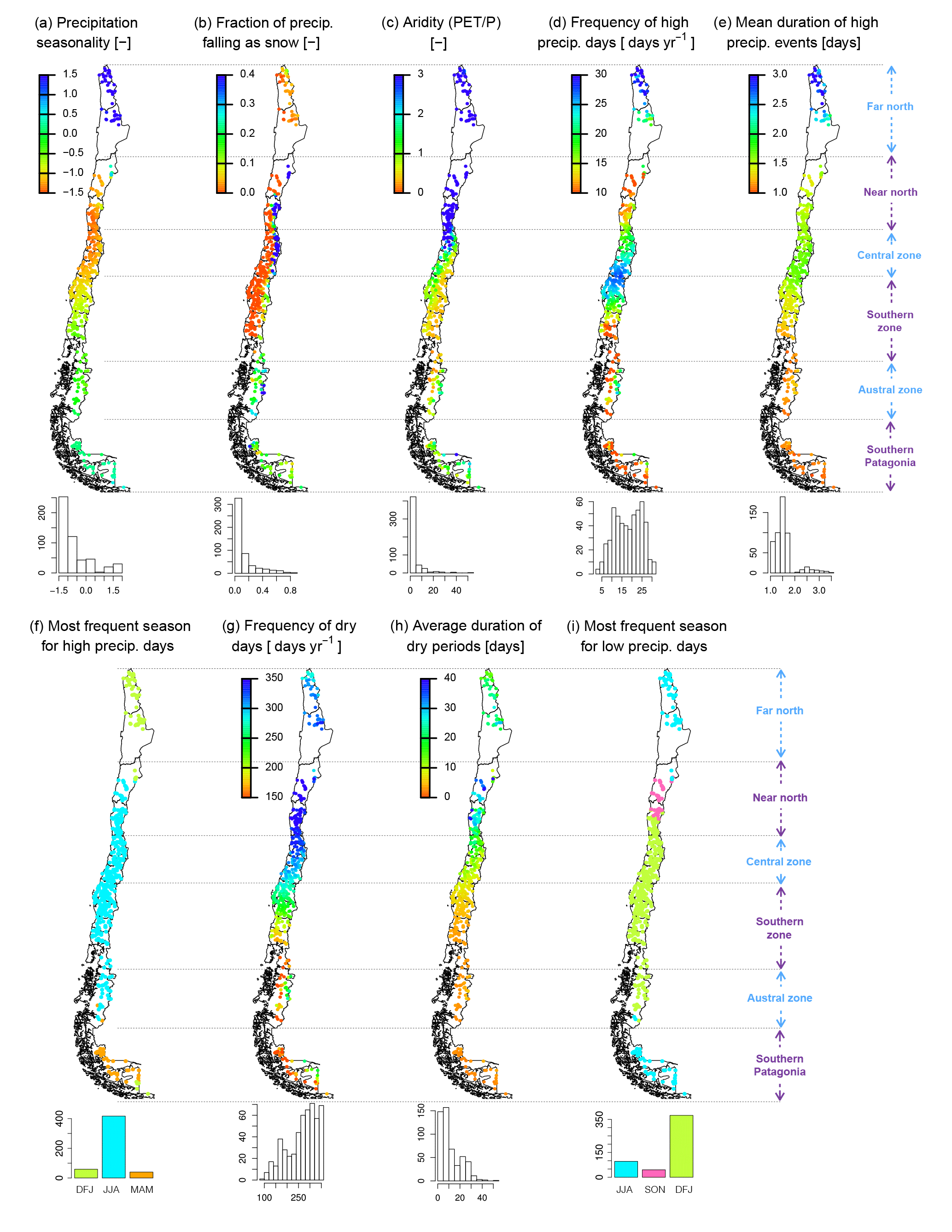
Figure 9Climatic indices (calculated from the precipcr2met product). The histograms indicate the number of catchments (out of 516) in each bin.
3.2.5 Hydrological signatures
Hydrological signatures were computed for the period 1 April 1990 to 31 March 2010, as in Sect. 3.2.4. To exclude the effects of anthropic intervention on hydrologic response, we selected 94 catchments with valid daily streamflow records in at least 85 % of the period, based on the following criteria: interv_degree lower than 0.1 (i.e. less than 10 % of the annual streamflow allocated to surface rights), large_dam equal to zero (absence of large dams within the catchment), imp_frac lower than 5 % (negligible urban areas), copr_frac lower than 20 % (negligible irrigation effects) and fp_frac lower than 20 % (negligible forest plantation effects). Further, we excluded glacier-dominated catchments by selecting glacier_frac lower than 5 %. It should be noted that, despite calculating hydrological indices for a subset of catchments, raw daily time series for all 516 catchments are included in the CAMELS-CL database. These time series and the formulae provided in Table 3 may be used if the signatures are required for different time periods.
Figure 10 illustrates the spatial distribution of 12 (out of 14) hydrological signatures (Table 3), revealing the leading patterns of catchment responses. Both mean daily flow and runoff ratio increase from the Far North to the Southern Zone, showing strong correlations with mean annual precipitation (Fig. 4b) and the aridity index (Fig. 9c). Further, the runoff ratio shows a positive west to east gradient (i.e. increase towards the Andes), reaching values above 1 in mountain catchments in the Southern Zone. These non-behavioural catchments are further analysed in Sect. 4.1. Mean half-flow dates (Fig. 10c) present a similar west to east gradient, with higher values in steep (Fig. 6c) snow-dominated (Fig. 9b) basins in central Chile – where the most frequent season for low-precipitation days is DJF (Fig. 9i).
The mid-segment slope of the flow duration curve (FDC, Fig. 10d) – a signature that quantifies flashiness of runoff – shows that slow basin-averaged responses occur in the Far North and part of the Near North, in spatial correspondence to a high baseflow index (Fig. 10e) and low discharge precipitation elasticity (Fig. 10f). Such behaviour is expected in this region due to substantial subsurface and groundwater contributions to total runoff. Although flashiness of runoff and discharge elasticity to precipitation (baseflow index) are relatively higher (lower) and show some correlation towards the south, no clear spatial gradients are observed within the domain spanning from central Chile to Southern Patagonia. Figure 10f shows negative elasticity values (−0.13 and −0.03) in two catchments located in the Austral Zone and Southern Patagonia. Such values indicate a negative annual runoff anomaly in response to the positive annual precipitation anomaly, which is not expected in near-natural catchments. We attribute this behaviour to two main factors. First, there is a numerical problem in the formula used to calculate streamflow elasticity (Eq. 7 in Sankarasubramanian et al., 2001, adapted in A17, Table 3) when annual precipitation of a single year approaches the long-term mean, causing the elasticity to approach infinity (Sankarasubramanian et al., 2001). A second factor is the use of incomplete streamflow daily records. Since the elasticity is computed from concurrent daily streamflow and precipitation, its calculation in catchments with missing streamflow records can be problematic. This can be particularly important in snow-dominated catchments (delayed runoff response to precipitation) and in catchments with a weak precipitation seasonality (i.e. precipitation falling during the whole year, Fig. 9a close to zero), which is the case for catchments in the Austral Zone and Southern Patagonia.
The examination of signatures related to extreme (high or low) streamflow conditions exposes some interesting features. Although no clear spatial relationship is observed between high-flow signatures (Fig. 10g–i), similar spatial distributions of low-flow frequencies (Fig. 10j) and mean low-flow durations (Fig. 10k) are obtained across the country. Q95 (Fig. 10i) and Q5 (Fig. 10l) provide generally similar patterns to those of mean daily discharge (Fig. 10a), with positive increases from the Far North to Southern zones, and a positive west to east gradient. The comparison between the signatures displayed in Fig. 10g–l and climatic indices in Fig. 9d–i highlights the complex relationship between climate and hydrologic catchment behaviour. For example, the spatial structure in the frequency of low-/high-precipitation days is not reflected in the spatial distribution of high-/low-flow frequencies. A similar disjunction is observed between the duration of low-precipitation (Fig. 9h) and low-flow (Fig. 10k) events, whereas those catchments with low-duration of high-precipitation events also provide low durations in high-flow events.
Sharp variations in hydrological signatures (Fig. 10) – in contrast to generally smooth patterns in climate indices (Fig. 9) – are the result of complex, non-linear processes across a range of spatiotemporal scales, enhanced by heterogeneities in topography, soils, vegetation, geology and other landscape properties. Careful attention should be paid to such interactions and to the uncertainties involved in the calculation of hydrological signatures, in particular when attempting to extrapolate hydrological behaviour from gauged to ungauged basins based on climatic similarities alone (Westerberg et al., 2016; Westerberg and McMillan, 2015).
3.2.6 Human intervention
Figure 11 summarises water rights records used to characterise human intervention degree within the catchments. We can see that the number of surface rights (Fig. 11a) increases from north to south, while the number of groundwater rights (Fig. 11d) increases from east to west. Although these values do not provide information about allocated volumes, they show how many water rights holders interact to coordinate water use within a particular catchment. The CAMELS-CL database provides information about each water right within a catchment (not only the attributes with synthesised information), in case more detailed analyses are required.
In terms of allocated surface and groundwater flows (Fig. 11b and e, respectively), we only considered consumptive permanent water rights. Further, we considered only water rights recorded as volume per time, since water rights expressed as “shares” (6 % of the national water rights database) were not provided with their corresponding conversion into volume units (DGA, 2016b). It should be noted that shares rights are the oldest (allocated prior to the 2005 water code reform), thus probably representing a majority of the rights within the Central Zone (the region that concentrates the oldest rights).
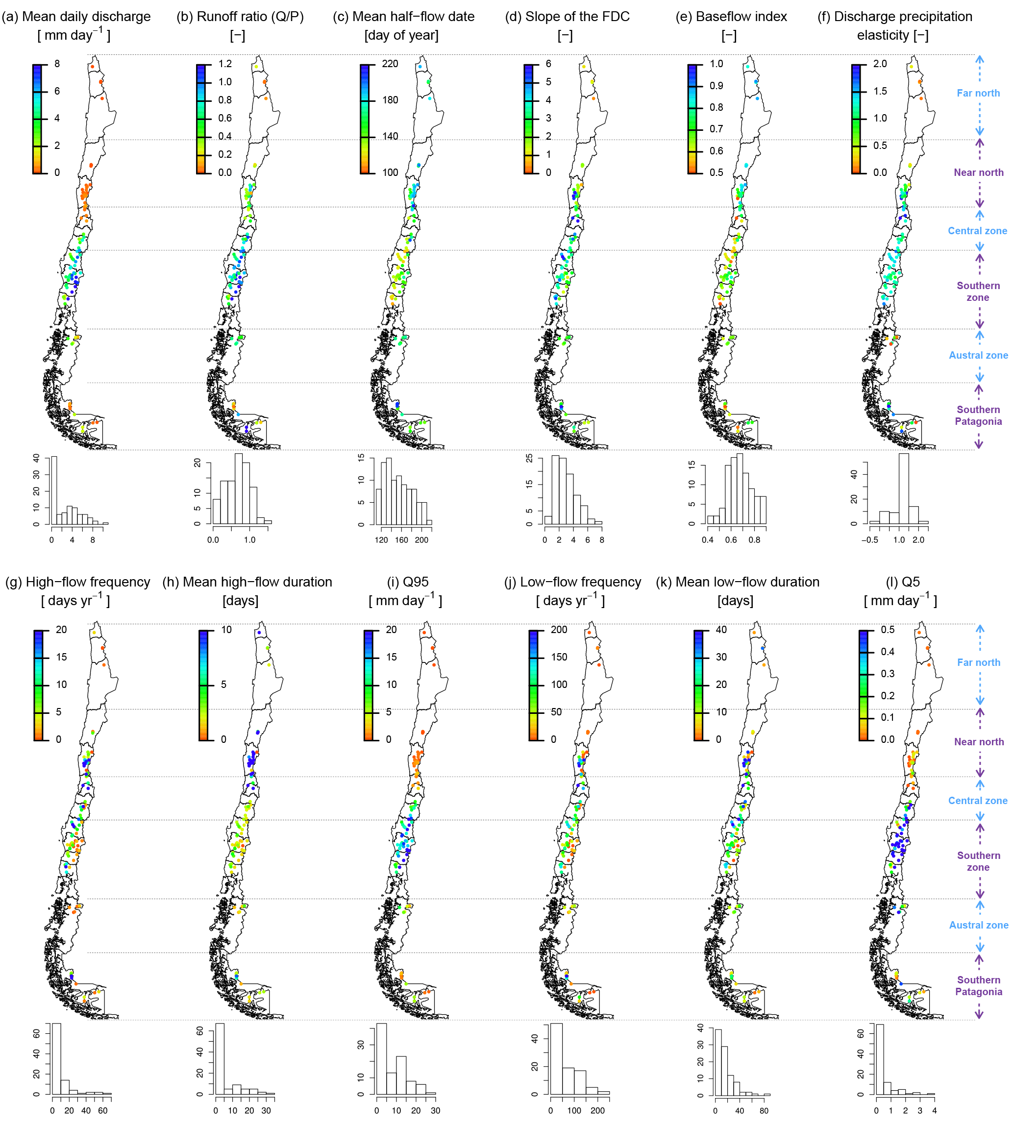
Figure 10Hydrologic signatures for 94 near-natural catchments. The histograms indicate the number of catchments (out of 94) in each bin.
The above limitations may lead to an underestimation of the allocated flow for (at least) the following reasons: (i) non-consumptive rights may have their restitution points outside the catchment boundaries (however, they were not considered for the allocated flow calculation); (ii) share rights are disregarded; (iii) there is missing information, and therefore some rights may be omitted (Sect. 3.1.10). On the other hand, allocation estimates may differ considerably from the actual extraction within a catchment. Possible reasons for this are the sub/over use of a granted allocated flow and unauthorised extractions of surface and groundwater.

Figure 11Water rights attributes. For visualisation purposes, the attributes in (a, b, d, e) are shown up to their 90th percentile. Attributes below the lower colour bar value are blank, and above the upper colour bar value they are blue. The histograms indicate the number of catchments (out of 516) in each bin.
Despite the limitations of the water use dataset and the attributes presented in Fig. 11, water rights information is critical to quantify human intervention, and it has not been officially processed at the catchment scale in Chile. To quantify the intervention degree within a catchment, we calculated the interv_degree attribute (described in Table 3 and illustrated in Fig. 11c) as the ratio between the annual surface flow allocated within a catchment and the catchment mean annual runoff. This attribute indicates how much of the annual runoff generated – on average – within a catchment corresponds to the water volume allocated as consumptive surface rights. Further, we defined a binary attribute to characterise the presence of reservoirs within a catchment (large_dam in Table 3), using 0 if there are no dams and 1 if there is at least one dam. A limitation of these human intervention attributes (interv_degree and large_dam) that should be considered for hydrological applications is that they do not incorporate information about groundwater extractions.
To quantify the urbanised fraction of a catchment – another important factor modulating catchment response – we used the impervious fractional area attribute (imp_frac in Table 3), which usually contains urban areas. However, this land cover type is the worst classified class, since urban areas have mixed pixels of vegetation and paved surfaces (Zhao et al., 2016). The urban fraction of the catchments (assumed to be equal to imp_frac) varied between 0 % and 7 % for most catchments (only one catchment had imp_frac = 25 %).
4.1 Precipitation assessment
To assess precipitation uncertainty, we looked at the inter-product differences across the study domain. To this end, we defined a precipitation spread attribute (p_mean_spread, Table 3) as the standard deviation of basin-averaged mean annual precipitation from the four different products, normalised by a multi-product mean. To allow such inter-comparison, we used data from the concurrent period 1998–2014 (Table 2) and excluded catchments located south of 50∘ S (since CHIRPS and TMPA cover up to 50∘ S). Given the different nature of the assessed precipitation products, the spread attribute can be interpreted as a measure of precipitation uncertainty. The underlying assumption is that similar values from different data sources indicate regions with higher confidence in precipitation estimates.
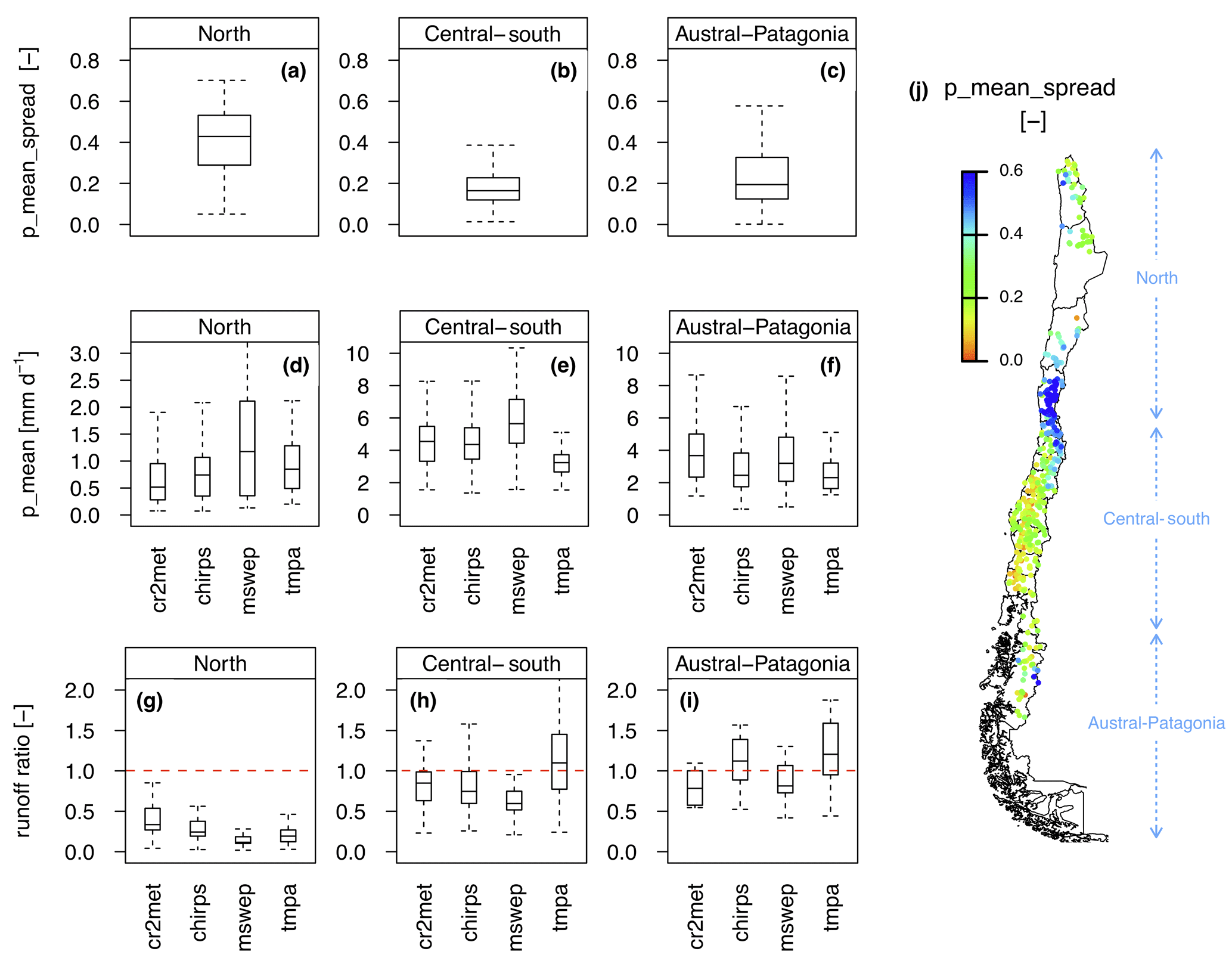
Figure 12Precipitation spread (p_mean_spread in a–c), mean annual precipitation (d–f), and runoff ratio (g–i) for the different precipitation products. The domain was divided into three main regions: North (north of 34∘ S); Central-South; and Austral-Patagonia. (j) shows the spatial distribution of p_mean_spread in these sub-regions.
Figure 12 displays catchment-scale mean precipitation and the precipitation spread index for three macro-regions: North (north of 34∘ S), which includes the Far North and Near North macro-zones; Central-South (between 34 and 43∘ S); and Austral-Patagonia (south of 43∘ S). Mean precipitation estimates (p_mean) have a larger spread in the North (Fig. 12a), indicating larger uncertainties in this domain. We attribute these higher relative errors to methodological challenges for detecting events and estimating their intensities in this arid sub-domain, where the occurrence of precipitation events is relatively rare (note the different scale used for p_mean in Fig. 12d). By contrast, considerably larger precipitation amounts (Fig. 12e and f) and lower spread values (Fig. 12b and c) are obtained in Central-South and Austral-Patagonia, which is expected given the relation of p_mean_spread to precipitation mean values. On the other hand, if we look at absolute inter-product differences (Fig. 12d–f), the Central-South region features the largest standard deviation in basin-averaged mean annual precipitation from the four different products (median value of 0.80 mm day−1, compared to 0.29 and 0.51 mm day−1 in the North and Austral-Patagonia regions, respectively). This is expected given the larger mean annual values over this humid region.
Although the effects of large precipitation uncertainty on streamflow modelling in the north are not straightforward to determine, some insights can be gained from our analyses. First, surface runoff is not very sensitive to variations in precipitation (i.e. small runoff elasticity values in Fig. 10f), suggesting a weak propagation of precipitation errors by hydrological models. Second, groundwater has the largest contribution to streamflow in this domain (the largest baseflow indices in Fig. 10e and sedimentary rocks as the most common geologic class illustrated in Fig. 7a), especially in the presence of Andean peatlands (represented by the wet_frac land cover attribute). This highlights the need to pursue a realistic representation of groundwater mechanisms in numerical models. Additionally, aquifer boundaries may be quite different from surface catchment boundaries, and therefore accurate delineations are needed to ensure a good representation of surface–groundwater interactions (e.g. Sar et al., 2015; Arkoprovo et al., 2012; Ivkovic et al., 2009).
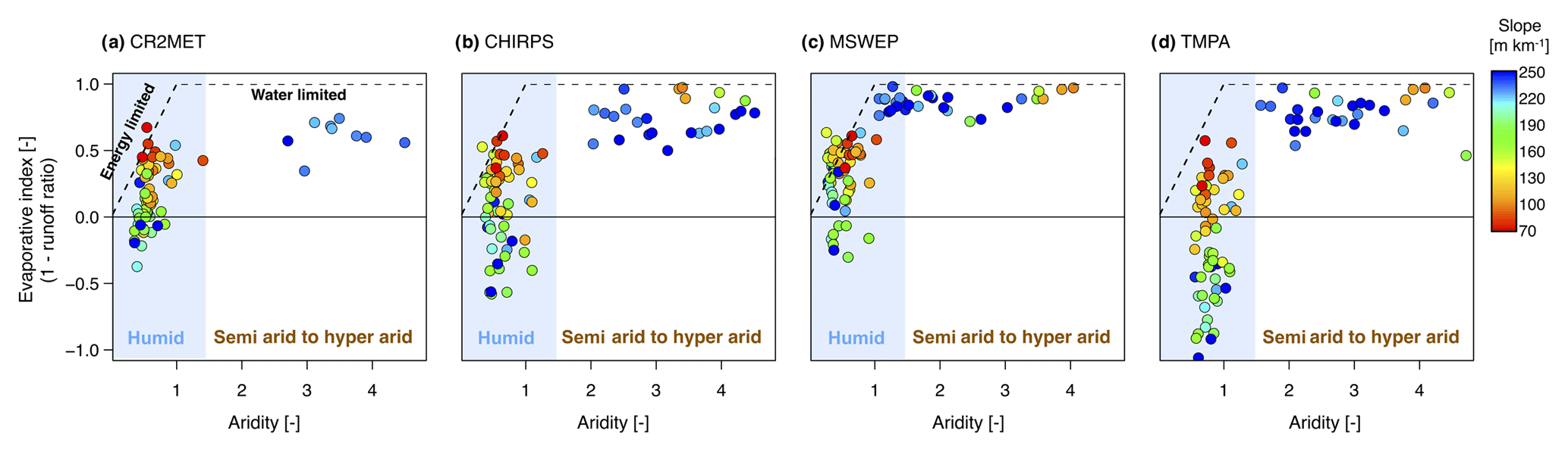
Figure 13Water balance for 94 near-natural catchments, illustrated in a Budyko scheme for CR2MET (a), CHIRPS (b), MSWEP (c), and TMPA (d). Markers are coloured by the catchment mean slope.
The ensemble spread of precipitation estimates is a measure of disagreement among the various products rather than a measure of accuracy, which should be quantified using ground observations (e.g. Zambrano-Bigiarini et al., 2017). Such analysis is beyond the scope of this paper, since the assessment of different precipitation products at the basin scale is typically conducted by forcing one or more hydrological models with the different precipitation datasets over the selected study area (e.g. Bisselink et al., 2016; Thiemig et al., 2013; Su et al., 2008).
As an alternative to the model-based approach, we examined the consistency of catchment precipitation estimates based on long-term runoff ratios in 94 near-natural catchments (Fig. 12g–i), selected following the criteria presented in Sect. 3.2.5. Although there are large inter-product differences in runoff ratios in the north (consistent with large p_mean_spread values in Fig. 12a), relatively low runoff ratio values (<0.4) are obtained, as expected given the arid and semi-arid conditions in this region. By contrast, there are catchments with runoff ratios larger than 1 in central–southern and Austral-Patagonia, indicating that there is more water leaving the catchment than the total amount entering as precipitation. Assuming that streamflow data and catchment area are reliable, and that changes in storage and groundwater contributions are negligible, such cases indicate precipitation underestimation by the various products. In the central–southern (Austral-Patagonia) region, the MSWEP (CR2MET) dataset provides 8 % (20 %) of catchment runoff ratios > 1 – i.e. the smallest among all products. In both domains, the TMPA dataset provides the largest fraction of catchments with runoff ratios > 1 (54 % in central–southern and 70 % in Austral-Patagonia). Such underestimation of TMPA, as well as other satellite precipitation estimates, was also reported by Hobouchian et al. (2017) and Zambrano-Bigiarini et al. (2017).
To further explore differences and systematic biases within the assessed products, we used the Budyko framework (Budyko, 1971) to diagnose the factors affecting the quality of the precipitation datasets. This framework links climate to catchment runoff and evapotranspiration in a simple and easy to interpret visualisation. Figure 13 shows the evaporative index (EI, the ratio of mean annual evapotranspiration to the mean annual precipitation), estimated as 1 minus the runoff ratio (i.e. assuming that changes in storage and groundwater contributions are negligible; Sposito, 2017), as a function of the aridity index for the 94 near-natural catchments over the period 1998–2014. Figure 13 illustrates how the evapotranspiration and runoff rates within this highly diverse set of catchments are governed by the available energy and precipitation; e.g. – for a given amount of precipitation – runoff exceeds evapotranspiration when the available energy and PET are relatively low (points below the energy-limited line in humid regions).
Negative EI values in Fig. 13 represent non-behavioural combinations of precipitation and runoff (Berghuijs et al., 2017). Under the assumption that precipitation estimates represent a relatively larger source of uncertainty compared to runoff, all the points with EI < 0 indicate those catchments where mean annual precipitation is underestimated (i.e. runoff ratios > 1). Therefore, Fig. 13a–d indicate that all precipitation products systematically fail in humid catchments with steep topography (slopes greater than 150 m km−1), in agreement with the limitations reported for different satellite precipitation products over the same domain (Hobouchian et al., 2017). The systematic precipitation underestimation can be attributed to the complex topography of headwater catchments and the scarcity of ground stations at high elevations. In fact, 90 % of the 500 rain gauges located south of 34∘ S are placed below 1000 m a.s.l. These precipitation errors pose challenges for hydrological applications, and the best strategy to address this will depend on the application. It should be noted that 57 catchment attributes (out of 70) and six hydro-meteorological time series (streamflow, min, max and mean temperature, PET, and SWE) do not rely on precipitation. Therefore, some applications may not need to directly address this limitation (e.g. catchment characterisation, water allocation analysis, classification studies not using similarity of climatic indices). Nevertheless, other applications (e.g. hydrological modelling) will have to deal with the uncertainties of this forcing variable. There are strategies for this, including setting up a parameter calibration scheme flexible enough to compensate for errors in meteorological input data (Elsner et al., 2014), or trying to correct precipitation estimates based on streamflow (Henn et al., 2015) and snow observations (Henn et al., 2016).
4.2 PET assessment
To assess the quality of the PET products described in Sect. 3.1.8, we used a different approach than in Sect. 4.1, since a basin-scale PET estimation cannot be evaluated based on observed streamflow. In this case, the evaluation was made with an independent set of PET data, calculated with daily observations for the period 2010–2014 from 75 meteorological stations maintained by the Chilean National Institute of Agricultural Research (INIA, 2017). For each site, we calculated two PET time series: (i) a daily time series obtained through the Hargreaves formulae (Hargreaves and Allen, 2003) fed with INIA temperature observations, called INIAhar hereafter, and (ii) an 8-day accumulated time series based on the FAO Penman–Monteith reference crop evapotranspiration (Allen et al., 1998), called INIA. INIAhar and INIA were used to evaluate the corresponding pixels of PEThar and PETmod, respectively.
The evaluation metrics used in these comparisons, spatially averaged within the macro-zones, are summarised in Table 4. These results indicate good agreement between PEThar and INIAhar, with correlation coefficients (r) greater than 0.92 throughout the national territory, except in the Far North macro-zone, where we found a weaker correlation (r=0.76). The ratios between mean PEThar and mean INIAhar indicate that PEThar underestimates (overestimates) by up to 8 % the observation-based PET in the Far and Near North arid regions (the Southern and Austral zones' humid regions).
The comparison between PETmod and INIA led to r values greater than 0.80 within the domain, excepting the Far North, where the correlation was below 0.20 in all available stations. The ratios between PETmod and INIA means indicate that the first one systematically overestimates station-based calculations, which was also found by Westerhoff (2015). Such systematic biases may be explained by the theoretical differences between INIA and PETmod calculated in MOD16. INIA represents a potential condition for a regular crop height of 0.12 m and a fixed surface resistance and albedo, which is not the case for PETmod, which includes a more complete parameterisation of those variables based on vegetation characteristics. Further, INIA uses local meteorological observations, while PETmod uses global sources that may not capture meteorological variations at the local scale. If an application requires it (e.g. irrigation or hydrological modelling applications), the reported PETmod biases can be corrected with conventional statistical methods (e.g. Maraun and Widmann, 2018). Other spatio-temporal analyses (e.g. drought monitoring) may directly apply PETmod due to its high correlation with ground ET0 estimates.
Table 4Evaluation metrics of PET gridded products (PEThar and PETmod). Pearson correlation coefficients (r) and the ratios between gridded PET and observation-based PET (INIAhar and INIA) were spatially averaged within the macro-zones.
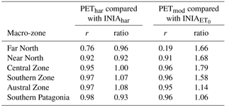
Since INIA records were used differently for evaluating PEThar and PETmod, a direct comparison between both assessments is not possible, although they provide valuable information about the quality of PET products across the territory. Furthermore, the formulations behind the two gridded products have different trade-offs. PETmod is based on the Penman–Monteith equation that solves the surface energy balance, including parameters such as albedo and FPAR/LAI, whereas PEThar is calculated from an empirical approach based only on air temperature. PEThar has a coarser spatial resolution (5×5 km2) compared to PETmod (×1 km2), which may induce larger errors over complex topography (e.g. mountain catchments) due to the local variations in potential evapotranspiration, with changes in slope and aspect. On the other hand, PEThar covers a longer period (1979–2016, the same as Tmin and Tmax from Sect. 3.1.7) compared to PETmod (2000–2014), which is more suitable for characterising climatic trends.
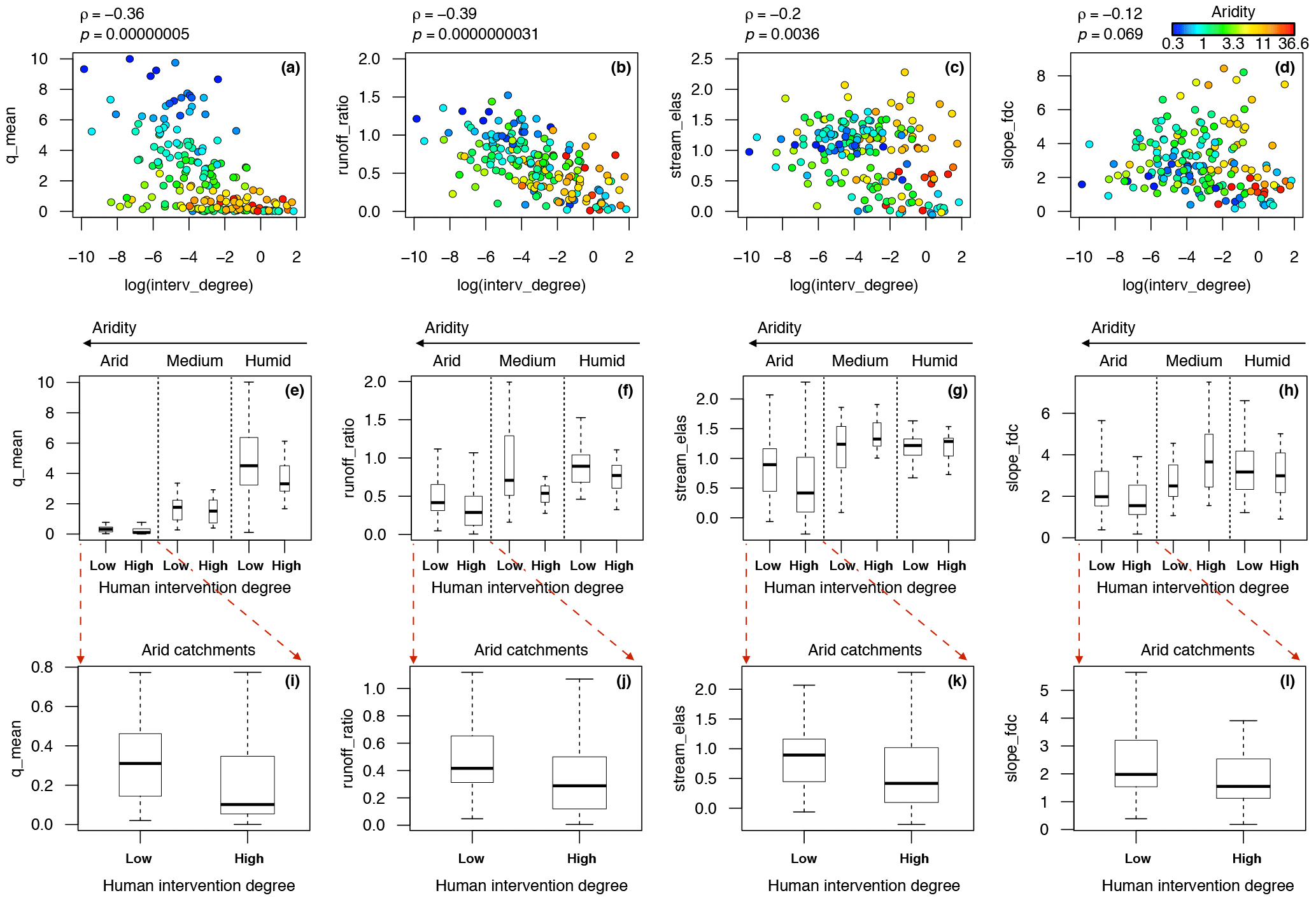
Figure 14(a)–(d) present the relation between four hydrological signatures and the log-transformed human intervention degree (“interv_degree” from Table 3). The Spearman rank correlation coefficients and their p values at 95 % confidence are shown in each plot. The colour corresponds to the aridity index. (e)–(h) show the boxplots (box widths are proportional to the number of catchments in each box) of the hydrological signatures for the catchments classified by their aridity (humid: aridity below 0.8, medium: aridity between 0.8 and 1.5, and arid: aridity above 1.5) and by their human intervention degree (low: interv_degree below 5 %, and high: interv_degree greater than 5 %). (i)–(l) present a zoomed view of the arid catchments.
Large sample hydrology is a suitable framework to explore anthropic impacts on catchment behaviour through comparative analysis over a broad range of hydroclimatic conditions and catchment characteristics. Such assessment is critical when addressing the question of how climate change will affect global water supply (Vörösmarty et al., 2007). However, it remains unclear how to generalise the results from different studies. For example, Poff et al. (2006) examined the effects of land use on hydrological regimes (e.g. peak and low flows, runoff variability) in 158 basins within the CONUS, finding region-dependent changes in specific metrics. Ochoa-Tocachi et al. (2016) analysed the impacts of land use on the hydrology of 25 Andean catchments, finding that anthropogenic influences propagate towards increased streamflow variability and decreased catchment regulation capacity and water yield. More recently, Tijdeman et al. (2018) examined the effects of human intervention on streamflow drought characteristics across 187 catchments in England and Wales, concluding that most human-influenced catchments did not have drought characteristics different from those expected for near-natural conditions.
In this work, we used hydrological signatures to describe catchment behaviour and the interv_degree attribute (Sect. 3.2.6) to characterise the level of human intervention. Figure 14a–d display scatter plots between four hydrological signatures and the logarithm of the intervention degree index – which accounts for consumptive, continuous surface water rights. Different colours indicate the aridity of each catchment, which is a major driver of hydrological behaviour (as shown in Fig. 13). These plots show that larger human intervention is associated with decreased annual flows and runoff ratios, especially in drier catchments. Interestingly, a larger number of consumptive surface rights (larger interv_degree values) is reflected in decreased elasticity of runoff with respect to precipitation, supported by low p values. Since these scatter plots do not allow one to separate the effects of aridity and human intervention, we binned the data and used boxplots to disentangle such effects. Figure 14e–h show the boxplots with these hydrological signatures for the classified catchments, binned according to their aridity (humid: aridity below 0.8, medium: aridity between 0.8 and 1.5, and arid: aridity above 1.5) and their degree of human intervention. Catchments with low (high) intervention were defined by the interv_degree values lower (greater) than 5 % and the large_dam attribute equal to 0 (1).
The dispersion in hydrological signatures among wet and medium catchments is large, and no significant difference is found between catchments with high and low human intervention. In contrast, dry catchments (zoomed view in Fig. 14i–l) reveal differences in hydrological signatures for high and low human intervention (i.e. median values in highly disturbed catchments are below the first quartile of low intervention catchments). In agreement with the scatter plots, the annual flows (Fig. 14i) and runoff ratios (Fig. 14j) decrease in catchments with larger numbers of consumptive surface rights, which is expected due to withdrawals of water within water-scarce regions. Further, highly disturbed arid catchments feature lower runoff sensitivities to precipitation compared to less disturbed ones (Fig. 14k), which could be attributed to altered runoff generation mechanisms associated with water withdrawals and reservoirs. Figure 14l shows that there is likely less variation in daily runoff – represented by the mid-segment slope of the flow duration curves – within highly disturbed arid catchments. The results found in arid catchments (i.e. water-scarce regions) provide new evidence of the potential impacts of human intervention on water supply. However, further research is needed to assess the causality of the correlations found here.
The CAMELS-CL dataset presented here provides novel information at the catchment scale in Chile, within a region that is largely underrepresented in large sample studies. CAMELS-CL includes daily streamflow data and a suite of basin-averaged hydro-meteorological variables, including precipitation, temperature, potential evapotranspiration, and snow water equivalent, for 516 catchments in the country. The dataset also includes shapefiles of drainage area boundaries related to streamflow gauge locations, overcoming the main limitations of the official national hydrographic network (DGA and CIREN, 2014). Further, we synthesised diverse and complementary datasets to compute 70 catchment attributes describing topography, geology, land cover, climate, hydrology, and anthropic intervention.
We described the advantages and main limitations of the datasets used to derive the various catchment attributes, which should be considered when using CAMELS-CL for selecting catchments and interpreting results. The main spatial patterns of catchment attributes and their inter-relationships were analysed across the entire domain (4300 km), which includes high-altitude catchments and five different primary climatic regimes. The main conclusions of this analysis are as follows:
-
the Andes position along the country largely explains the elevation and slope gradients from the 516 catchments,
-
there is high geological variability between neighbouring catchments and within catchments,
-
there is larger heterogeneity in land cover attributes towards southern regions,
-
48 % of the catchments have some degree of glacierisation,
-
the climatic attributes show a marked north to south precipitation gradient, combined with an orographic enhancement over the windward slope of the Andes Cordillera,
-
hydrological signatures reflect the leading patterns of catchment hydrologic responses, with strong correlations between runoff (daily flows and runoff ratios) and mean annual precipitation and aridity index,
-
there are substantial subsurface and groundwater contributions to total runoff in the northern regions (Far North and Near North), and
-
hydrological signatures feature, in general, sharper variations compared to patterns in climate indices, which is due to complex process interactions across a range of spatiotemporal scales, enhanced by heterogeneities in topography, soils, vegetation, geology and other landscape properties, and data errors (as also observed in the USA by Addor et al., 2018).
The CAMELS-CL dataset was further used to assess hydro-meteorological biases and uncertainties in a large ensemble of watersheds in Chile, based on the comparison of various precipitation products – one national (CR2MET) and three widely used global products (CHIRPS, MSWEP and TMPA). Large discrepancies between products were detected in arid regions, which are explained by the methodological challenges associated with the rare occurrence of precipitation events in this region. Based on a water balance analysis using Budyko curves, we found systematic precipitation underestimation in headwater mountain catchments (high elevations and steep slopes) over humid regions. For these topographic characteristics and climatic conditions, all products failed to provide precipitation estimates that closed the water balance, with the TMPA product featuring the largest errors – in agreement with previous studies over the same domain (Hobouchian et al., 2017; Zambrano-Bigiarini et al., 2017). Such errors were attributed to the complex topography of headwater catchments and the scarcity of ground stations at high elevations (90 % of rain gauges located south of 34∘ S are placed below 1000 m a.s.l.). These limitations restrict our understanding of hydrological processes, posing challenges for streamflow modelling, water management and allocation. To alleviate these constraints, efforts should be put into improving the surface monitoring network at high elevations (>1000 m a.s.l.). This would help to obtain more accurate remotely sensed and model-based precipitation estimates in complex terrains. To deal with these precipitation errors in hydrological applications, we suggest exploring suitable strategies based on application requirements and using our findings to better interpret results. Further, we assessed the PEThar and PETmod products with an independent observation-based PET. In general, both products showed good correlations with the observation-based PET for the complete domain, except in the Far North arid region. Regarding mean biases, PEThar showed slight underestimation (overestimation) in the Far and Near North arid regions (the Southern and Austral zones' humid regions) compared with the observation-based PET. PETmod on the other hand showed a systematic and larger overestimation of the observation-based PET within the complete domain, which was attributed to the theoretical differences between their formulations.
The assessment of precipitation and PET products showed different performances within the domain. Therefore, the choice of these products or similar datasets must be carefully made based on specific application and study requirements.
Finally, we used CAMELS-CL to explore the impact of human activities on catchment behaviour. We showed that larger human intervention is correlated with lower than normal annual flows, runoff ratios, elasticity of runoff with respect to precipitation, and flashiness of runoff, especially in drier catchments. These results not only illustrate how catchment behaviour can change with human intervention, but also reveal the potential of anthropic indices to explain shifts in hydrological systems.
In summary, this paper contributes to hydrological sciences by (i) providing a unique dataset that can be used to advance our understanding of hydrological systems by learning from diversity, (ii) analysing the dominant spatial patterns of physical, climatic and hydrological attributes within the domain, (iii) assessing the quality of one national and three global precipitation datasets based on the observed water balance, (iv) assessing two PET products based on an independent set of PET point values calculated from meteorological records, and (v) examining the interplay between human intervention and changes in observed catchment response.
CAMELS-CL can be used to address research questions related to catchment classification, similarity and regionalisation, model parameter estimation, dominant controls on runoff generation, the impacts of different land cover types on catchment response, characterisation of drought history and projections, and climate change impacts on hydrological processes. CAMELS-CL will be continuously updated to incorporate new records and new datasets, which may include soil characteristics, water quality, seismology records, socio-economic indices and energy generation data. Additionally, new and more detailed information about the Chilean cryosphere will be included, complementing the global inventory processed here with national inventories of Chile and Argentina. Time series of streamflow, meteorological variables, and all catchment attributes described in this paper can be visualised from the CAMELS-CL explorer (http://camels.cr2.cl, last access: November 2018) and downloaded from https://doi.pangaea.de/10.1594/PANGAEA.894885 (last access: Novemmber 2018).
ASTER GDEM elevation data were downloaded from the NASA-JPL website (https://asterweb.jpl.nasa.gov/gdem.asp; ASTER GDEM, 2016). Geological data (GLiM) were downloaded from the PANGAEA database (https://doi.pangaea.de/10.1594/PANGAEA.788537; GLiM, 2017). The land cover map was downloaded from the Universidad de Chile website (http://www.gep.uchile.cl/Landcover_CHILE.html; Land cover map, 2017). Glaciers inventory RGI 6.0 was downloaded from the Global Land Ice Measurements from Space initiative (https://www.glims.org/RGI; Glaciers inventory, 2017). The daily streamflow records were obtained from the CR2 website (http://www.cr2.cl/datos-de-caudales; Streamflow, 2018). CR2MET precipitation and temperature products were downloaded from the CR2 website (http://www.cr2.cl/datos-productos-grillados; Precipitation product CR2MET, 2018). CHIRPS, TMPA and MSWEP precipitation products are publicly available and the datasets clipped within the Chilean domain were downloaded from the CR2 website (http://www.cr2.cl/datos-precipitacion-satelital; Satellite precipitation products CHIRPS, MSWEP, TMPA, 2018). MODIS data were downloaded from the USGS website (https://e4ftl01.cr.usgs.gov/MOLT; MODIS, 2017). SWE data were provided by Gonzalo Cortes (Cortés et al., 2016). Water rights were downloaded from the DGA website (http://www.dga.cl/productosyservicios/derechos_historicos; Water rights, 2018). Dam location was downloaded from the Ministerio de Bienes Nacional website (http://www.ide.cl/descarga/capas/item/embalses-2016.html, Dam location, 2017). The time series processed at the basin scale and the catchment attributes introduced in this paper are freely available from https://doi.pangaea.de/10.1594/PANGAEA.894885 and the CAMELS-CL explorer (http://camels.cr2.cl).
This research was conceived by CAG, PAM and JPB. CAG processed the catchment attributes and designed and wrote the manuscript with input from all co-authors. PAM performed the analysis of hydrological signatures. JPB developed and processed the CR2MET products. JPB and RG performed the analysis of climatic indices. NA provided R codes for computing climatic indices and hydrological signatures, and performed the analysis on geological attributes. MG and CP performed the analysis on PET. MZB processed the satellite precipitation products. AL contributed with the analysis of land cover attributes. GC processed the SWE data. JM contributed ideas for analyses. AA processed the glacier data. All the authors have been involved in interpreting the results, discussing the findings, and editing the paper.
The authors declare that they have no conflict of interest.
This research emerged from the collaboration with many colleagues at the
Center for Climate and Resilience Research (CR2, CONICYT/FONDAP/15110009).
Camila Alvarez-Garreton is funded by FONDECYT postdoctoral grant no. 3170428.
Pablo Mendoza received additional support from FONDECYT postdoctoral grant
no. 3170079. Mauricio Zambrano-Bigiarini thanks FONDECYT 11150861 for
financial support. The development of CR2MET was supported by the Chilean
Water Directorate (DGA), through National Water Balance Updating
Project DGA-2319, and by FONDECYT grant no. 3150492. This study is a
contribution to the Large-sample Hydrology working group of the Panta Rhei
Research Initiative of the International Association of Hydrological
Sciences (IAHS). We thank Guillermo Tapia from the DGA for his advice on
stream-gauge locations.
Edited by:
Jan Seibert
Reviewed by: Margarita Saft and three anonymous
referees
Addor, N., Newman, A. J., Mizukami, N., and Clark, M. P.: The CAMELS data set: Catchment attributes and meteorology for large-sample studies, Hydrol. Earth Syst. Sci., 21, 5293–5313, https://doi.org/10.5194/hess-21-5293-2017, 2017.
Addor, N., Nearing, G., Prieto, C., Newman, A. J., Le Vine, N., and Clark, M. P.: A ranking of hydrological signatures based on their predictability in space, Water Resour. Res., 54, https://doi.org/10.1029/2018WR022606, 2018.
Adler, R. F., Huffman, G. J., Chang, A., Ferraro, R., Xie, P.-P., Janowiak, J., Rudolf, B., Schneider, U., Curtis, S., Bolvin, D., Gruber, A., Susskind, J., Arkin, P., and Nelkin, E.: The Version-2 Global Precipitation Climatology Project (GPCP) Monthly Precipitation Analysis (1979–Present), J. Hydrometeorol., 4, 1147–1167, https://doi.org/10.1175/1525-7541(2003)004<1147:TVGPCP>2.0.CO;2, 2003.
Allen, R. G., Pereira, L. S., Raes, D., and Smith, M.: FAO Penman–Monteith Equation, in: Crop Evapotranspiration: Guidelines for Computing Crop Water Requirements, FAO – Food and Agriculture Organization of the United Nations, Rome, 17–28, 1998.
Allmendinger, R. W., Jordan, T. E., Kay, S. M., and Isacks, B. L.: The evolution of the Altiplano-Puna Plateau of the Central Andes, Annu. Rev. Earth Planet. Sci., 25, 139–174, https://doi.org/10.1146/annurev.earth.25.1.139, 1997.
Andréassian, V., Hall, A., Chahinian, N., and Schaake, J.: Introduction and Synthesis: Why should hydrologists work on a large number of basin data sets?, IAHS-AISH Publ., 307, 1–6, 2006.
Arkoprovo, B., Adarsa, J., and Prakash, S. S.: Delineation of Groundwater Potential Zones using Satellite Remote Sensing and Geographic Information System Techniques: A Case study from Ganjam district, Orissa, India, Res. J. Recent Sci., 1, 59–66, 2012.
Armesto, J. J., Manuschevich, D., Mora, A., Smith-Ramirez, C., Rozzi, R., Abarzúa, A. M., and Marquet, P. A.: From the Holocene to the Anthropocene: A historical framework for land cover change in southwestern South America in the past 15,000 years, Land Use Policy, 27, 148–160, https://doi.org/10.1016/j.landusepol.2009.07.006, 2010.
ASTER GDEM: https://asterweb.jpl.nasa.gov/gdem.asp, last access: December 2016.
Balsamo, G., Albergel, C., Beljaars, A., Boussetta, S., Brun, E., Cloke, H., Dee, D., Dutra, E., Munõz-Sabater, J., Pappenberger, F., De Rosnay, P., Stockdale, T., and Vitart, F.: ERA-Interim/Land: A global land surface reanalysis data set, Hydrol. Earth Syst. Sci., 19, 389–407, https://doi.org/10.5194/hess-19-389-2015, 2015.
Beck, H. E., Van Dijk, A. I. J. M., Levizzani, V., Schellekens, J., Miralles, D. G., Martens, B., and De Roo, A.: MSWEP: 3-hourly 0.25∘ global gridded precipitation (1979–2015) by merging gauge, satellite, and reanalysis data, Hydrol. Earth Syst. Sci., 21, 589–615, https://doi.org/10.5194/hess-21-589-2017, 2017.
Berghuijs, W. R., Sivapalan, M., Woods, R. A., and Savenije, H. H. G.: Patterns of similarity of seasonal water balances: A window into streamflow variability over a range of time scales, Water Resour. Res., 50, 5638–5661, https://doi.org/10.1002/2014WR015692, 2014.
Berghuijs, W. R., Larsen, J. R., van Emmerik, T. H. M., and Woods, R. A.: A Global Assessment of Runoff Sensitivity to Changes in Precipitation, Potential Evaporation, and Other Factors, Water Resour. Res., 53, 8475–8486, https://doi.org/10.1002/2017WR021593, 2017.
Bisselink, B., Zambrano-Bigiarini, M., Burek, P., and de Roo, A.: Assessing the role of uncertain precipitation estimates on the robustness of hydrological model parameters under highly variable climate conditions, J. Hydrol. Reg. Stud., 8, 112–129, https://doi.org/10.1016/j.ejrh.2016.09.003, 2016.
Blöschl, G., Sivapalan, M., Wagener, T., Viglione, A., and Savenije, H.: Runoff Prediction in Ungauged Basins: Synthesis Across Processes, Places and Scales, Cambridge University Press, Cambridge, 2013.
Budyko, M. I.: Climate and Life, Academic Press, London, 1971.
Carey: General Overview of Water Rights in Chile, available at: http://reformacodigodeaguas.carey.cl/wp-content/uploads/2014/09/general-explanation-of-the-chilean-water (last access: May 2018), 2014.
Cortés, G. and Margulis, S.: Impacts of El Niño and La Niña on interannual snow accumulation in the Andes: Results from a high-resolution 31 year reanalysis, Geophys. Res. Lett., 44, 6859–6867, https://doi.org/10.1002/2017GL073826, 2017.
Cortés, G., Girotto, M., and Margulis, S. A.: Analysis of sub-pixel snow and ice extent over the extratropical Andes using spectral unmixing of historical Landsat imagery, Remote Sens. Environ., 141, 64–78, https://doi.org/10.1016/j.rse.2013.10.023, 2014.
Cortés, G., Girotto, M., and Margulis, S.: Snow process estimation over the extratropical Andes using a data assimilation framework integrating MERRA data and Landsat imagery, Water Resour. Res., 52, 2582–2600, https://doi.org/10.1002/2015WR018376, 2016.
Dam location: http://www.ide.cl/descarga/capas/item/embalses-2016.html, last access: September 2017.
DGA: Mapa Hidrogeológico de Chile, Santiago, Chile, 1986.
DGA: Glaciares de chile, Santiago, Chile, 2014.
DGA: Atlas del Agua – Chile 2016, in: Capítulo 1: Chile en el mundo, Atlas del Agua Chile 2016, Santiago, Chile, 24 pp., 2016a.
DGA: Atlas del Agua – Chile 2016, in Capítulo 4: Gestion del agua, Atlas del Agua Chile 2016, Santiago, Chile, 30 pp., 2016b.
DGA: Actualización del Balance Hídrico Nacional, SIT No. 417, Ministerio de Obras Públicas, Dirección General de Aguas, División de Estudios y Planificación, Santiago, Chile, Realizado por: Universidad de Chile & Pontificia Universidad Católica de Chile, 2017.
DGA and CIREN: Redefinición de la clasificación red hidrográfica a nivel Nacional, Santiago, Chile, 2014.
Di Gregorio, A. and Jansen, L. J.: Land Cover Classification System, Classification concepts and user manual, FAO – Food and Agriculture Organization of the United Nations, Rome, 2005.
Ehret, U., Gupta, H. V., Sivapalan, M., Weijs, S. V., Schymanski, S. J., Blöschl, G., Gelfan, A. N., Harman, C., Kleidon, A., Bogaard, T. A., Wang, D., Wagener, T., Scherer, U., Zehe, E., Bierkens, M. F. P., Di Baldassarre, G., Parajka, J., Van Beek, L. P. H., Van Griensven, A., Westhoff, M. C., and Winsemius, H. C.: Advancing catchment hydrology to deal with predictions under change, Hydrol. Earth Syst. Sci., 18, 649–671, https://doi.org/10.5194/hess-18-649-2014, 2014.
Elsner, M. M., Gangopadhyay, S., Pruitt, T., Brekke, L. D., Mizukami, N., and Clark, M. P.: How Does the Choice of Distributed Meteorological Data Affect Hydrologic Model Calibration and Streamflow Simulations?, J. Hydrometeorol., 15, 1384–1403, https://doi.org/10.1175/JHM-D-13-083.1, 2014.
Figueroa, D. and Moffat, C.: On the influence of topography in the induction of coastal upwelling along the Chilean coast, Geophys. Res. Lett., 27, 3905–3908, https://doi.org/10.1029/1999GL011302, 2000.
Friedl, M., McIver, D., Hodges, J. C., Zhang, X., Muchoney, D., Strahler, A., Woodcock, C., Gopal, S., Schneider, A., Cooper, A., Baccini, A., Gao, F., and Schaaf, C.: Global land cover mapping from MODIS: algorithms and early results, Remote Sens. Environ., 83, 287–302, https://doi.org/10.1016/S0034-4257(02)00078-0, 2002.
Funk, C., Peterson, P., Landsfeld, M., Pedreros, D., Verdin, J., Shukla, S., Husak, G., Rowland, J., Harrison, L., Hoell, A., and Michaelsen, J.: The climate hazards infrared precipitation with stations – A new environmental record for monitoring extremes, Sci. Data, 2, 150066, https://doi.org/10.1038/sdata.2015.66, 2015.
Garreaud, R. D.: The Andes climate and weather, Adv. Geosci., 22, 3–11, https://doi.org/10.5194/adgeo-22-3-2009, 2009.
Garreaud, R. D., Alvarez-Garreton, C., Barichivich, J., Boisier, J. P., Christie, D., Galleguillos, M., LeQuesne, C., McPhee, J., and Zambrano-Bigiarini, M.: The 2010–2015 megadrought in central Chile: impacts on regional hydroclimate and vegetation, Hydrol. Earth Syst. Sci., 21, 6307–6327, https://doi.org/10.5194/hess-21-6307-2017, 2017.
Glaciers inventory: https://www.glims.org/RGI, last access: December 2017.
GLiM: https://doi.pangaea.de/10.1594/PANGAEA.788537, last access: May 2017.
Gong, P., Wang, J., Yu, L., Zhao, Y., Zhao, Y., Liang, L., Niu, Z., Huang, X., Fu, H., Liu, S., Li, C., Li, X., Fu, W., Liu, C., Xu, Y., Wang, X., Cheng, Q., Hu, L., Yao, W., Zhang, H., Zhu, P., Zhao, Z., Zhang, H., Zheng, Y., Ji, L., Zhang, Y., Chen, H., Yan, A., Guo, J., Yu, L., Wang, L., Liu, X., Shi, T., Zhu, M., Chen, Y., Yang, G., Tang, P., Xu, B., Giri, C., Clinton, N., Zhu, Z., Chen, J., and Chen, J.: Finer resolution observation and monitoring of global land cover: First mapping results with Landsat TM and ETM+ data, Int. J. Remote Sens., 34, 2607–2654, https://doi.org/10.1080/01431161.2012.748992, 2013.
Google: Google Earth Pro, Google, available at: https://www.google.com/earth/ (last access: March 2018), 2016.
Gupta, H. V., Perrin, C., Blöschl, G., Montanari, A., Kumar, R., Clark, M., and Andréassian, V.: Large-sample hydrology: A need to balance depth with breadth, Hydrol. Earth Syst. Sci., 18, 463–477, https://doi.org/10.5194/hess-18-463-2014, 2014.
Hargreaves, G. H. and Allen, R. G.: History and evaluation of Hargreaves evapotranspiration equation, J. Irrig. Drain. Eng., 129, 53–63, https://doi.org/10.1061/(ASCE)0733-9437(2003)129:1(53), 2003.
Hargreaves, G. H. and Samani, Z. A.: Reference crop evapotranspiration from temperature, Appl. Eng. Agric., 1, 96–99, https://doi.org/10.13031/2013.26773, 1985.
Hartmann, J. and Moosdorf, N.: The new global lithological map database GLiM: A representation of rock properties at the Earth surface, Geochem. Geophy. Geosy., 13, 1–37, https://doi.org/10.1029/2012GC004370, 2012.
Henn, B., Clark, M. P., Kavetski, D., and Lundquist, J. D.: Estimating mountain basin-mean precipitation fromstreamflow using Bayesian inference, Water Resour. Res., 51, 8012–8033, https://doi.org/0.1002/2014WR016736, 2015.
Henn, B., Clark, M. P., Kavetski, D., McGurk, B., Painter, T. H., and Lundquist, J. D.: Combining snow, streamflow, and precipitation gauge observations to infer basin-mean precipitation, Water Resour. Res., 52, 8700–8723, https://doi.org/10.1002/2015WR018564, 2016.
Hijmans, R. J.: Raster: Geographic Data Analysis and modeling, R Packag. version 2.5-8. https//CRAN.R-project.org/package=raster, 1, r948, 2016.
Hobouchian, M. P., Salio, P., García Skabar, Y., Vila, D., and Garreaud, R.: Assessment of satellite precipitation estimates over the slopes of the subtropical Andes, Atmos. Res., 190, 43–54, https://doi.org/10.1016/j.atmosres.2017.02.006, 2017.
Howell, T. and Evett, S. R.: The Penman–Monteith Method, Bushland, Texas, USDA Agric. Res. Serv., Texas, 1–13, 2001.
Huang, C., Newman, A. J., Clark, M. P., Wood, A. W., and Zheng, X.: Evaluation of snow data assimilation using the ensemble Kalman filter for seasonal streamflow prediction in the western United States, Hydrol. Earth Syst. Sci., 21, 635–650, https://doi.org/10.5194/hess-21-635-2017, 2017.
Huffman, G. J., Bolvin, D. T., Nelkin, E. J., Wolff, D. B., Adler, R. F., Gu, G., Hong, Y., Bowman, K. P., and Stocker, E. F.: The TRMM Multisatellite Precipitation Analysis (TMPA): Quasi-Global, Multiyear, Combined-Sensor Precipitation Estimates at Fine Scales, J. Hydrometeorol., 8, 38–55, https://doi.org/10.1175/JHM560.1, 2007.
Huffman, G. J., Adler, R. F., Bolvin, D. T., and Nelkin, E. J.: The TRMM Multi-satellite Precipitation Analysis (TMPA), in: Satellite Rainfall Applications for Surface Hydrology, Springer, Dordrecht, 3–22, 2010.
Huss, M. and Hock, R.: A new model for global glacier change and sea-level rise, Front. Earth Sci., 3, 54, https://doi.org/10.3389/feart.2015.00054, 2015.
IGM: Hidrografía, in: Geografía de Chile, Santiago, Chile, p. 19, 1984.
INIA: AGROMET, Instituto Nacional de Investigacion Agriola. Ministerio de Agricultura, available at: https://agromet.cl, last access: May 2017.
Ivkovic, K. M., Letcher, R. A., and Croke, B. F. W.: Use of a simple surface-groundwater interaction model to inform water management, Aust. J. Earth Sci., 56, 71–80, 2009.
Jin, Y., Schaaf, C. B., Woodcock, C., Gao, F., Li, X., and Strahler, A. H.: Consistency of MODIS surface bidirectional reflectance distribution function and albedo retrievals: 2. Validation, J. Geophys. Res., 108, 4159, https://doi.org/10.1029/2002JD002804, 2003.
Jones, J., Almeida, A., Cisneros, F., Iroumé, A., Jobbágy, E., Lara, A., de Lima, W. P., Little, C., Llerena, C., Silveira, L., and Villegas, J. C.: Forests and water in South America, Hydrol. Process., 31, 972–980, https://doi.org/10.1002/hyp.11035, 2017.
Kottek, M., Grieser, J., Beck, C., Rudolf, B., and Rubel, F.: World map of the Köppen–Geiger climate classification updated, Meteorol. Z., 15, 259–263, https://doi.org/10.1127/0941-2948/2006/0130, 2006.
Ladson, A., Bronw, R., Neal, B., and Nathan, R.: A standard approach to baseflow separation using the Lyne and Hollick filter, Tech. Pap., Aust. J. Water Resour., 17, 25–34, https://doi.org/10.7158/W12-028.2013.17.1, 2013.
La Moreaux, P. E., Wilson, B. M., and Memon, B. A.: Guide to the hydrology of carbonate rocks, Unesco – United Nations Educational, Scientific and Cultural Organization, Paris, 1984.
Land cover map: http://www.gep.uchile.cl/Landcover_CHILE.html, last access: May 2017.
Lara, A., Little, C., Urrutia, R., McPhee, J., Álvarez-Garretón, C., Oyarzún, C., Soto, D., Donoso, P., Nahuelhual, L., Pino, M., and Arismendi, I.: Assessment of ecosystem services as an opportunity for the conservation and management of native forests in Chile, Forest Ecol. Manage., 258, 415–424, https://doi.org/10.1016/j.foreco.2009.01.004, 2009.
Larraín, S.: El agua en Chile: entre los derechos humanos y las reglas del mercado, http://Polis.Revues.Org (last access: May 2018), 2006.
Le Quesne, C., Acuña, C., Boninsegna, J. A., Rivera, A., and Barichivich, J.: Long-term glacier variations in the Central Andes of Argentina and Chile, inferred from historical records and tree-ring reconstructed precipitation, Palaeogeogr. Palaeocl. Palaeoecol., 281, 334–344, https://doi.org/10.1016/j.palaeo.2008.01.039, 2009.
Liston, G. E.: Representing subgrid snow cover heterogeneities in regional and global models, J. Climate, 17, 1381–1397, https://doi.org/10.1175/1520-0442(2004)017<1381:RSSCHI>2.0.CO;2, 2004.
Lucht, W., Schaaf, C. B., and Strahler, A. H.: An algorithm for the retrieval of albedo from space using semiempirical BRDF models, IEEE T. Geosci. Remote, 38, 977–998, https://doi.org/10.1109/36.841980, 2000.
Maraun, D. and Widmann, M.: Statistical Downscaling and Bias Correction for Climate Research, Cambridge University Press, Cambridge, 170–200, 2018.
Margulis, S. A., Cortés, G., Girotto, M., and Durand, M.: A Landsat-Era Sierra Nevada Snow Reanalysis (1985–2015), J. Hydrometeorol., 17, 1203–1221, https://doi.org/10.1175/JHM-D-15-0177.1, 2016.
Marzeion, B., Jarosch, A. H., and Hofer, M.: Past and future sea-level change from the surface mass balance of glaciers, The Cryosphere, 6, 1295–1322, https://doi.org/10.5194/tc-6-1295-2012, 2012.
McDonnell, J. J. and Woods, R.: On the need for catchment classification, J. Hydrol., 299, 2–3, https://doi.org/10.1016/j.jhydrol.2004.09.003, 2004.
Melsen, L. A., Addor, N., Mizukami, N., Newman, A. J., Torfs, P. J. J. F., Clark, M. P., Uijlenhoet, R., and Teuling, A. J.: Mapping (dis)agreement in hydrologic projections, Hydrol. Earth Syst. Sci., 22, 1775–1791, https://doi.org/10.5194/hess-22-1775-2018, 2018.
Mernild, S. H., Liston, G. E., Hiemstra, C., and Wilson, R.: The Andes Cordillera. Part III: glacier surface mass balance and contribution to sea level rise (1979–2014), Int. J. Climatol., 37, 3154–3174, https://doi.org/10.1002/joc.4907, 2017.
Miller, A.: The climate of Chile, in: World survey of climatology, Elsevier, Amsterdam, 113–145, 1976.
Miranda, A., Altamirano, A., Cayuela, L., Pincheira, F., and Lara, A.: Different times, same story: Native forest loss and landscape homogenization in three physiographical areas of south-central of Chile, Appl. Geogr., 60, 20–28, https://doi.org/10.1016/j.apgeog.2015.02.016, 2015.
Mizukami, N., Clark, M. P., Newman, A. J., Wood, A. W., Gutmann, E. D., Nijssen, B., Rakovec, O., and Samaniego, L.: Towards seamless large-domain parameter estimation for hydrologic models, Water Resour. Res., 53, 8020–8040, https://doi.org/10.1002/2017WR020401, 2017.
MODIS: https://e4ftl01.cr.usgs.gov/MOLT, last access: May 2017.
Mu, Q., Zhao, M., and Running, S.: Brief Introduction to MODIS Evapotranspiration Data Set (MOD16), Water Resour. Res., 45, 0–4, 2005.
Myneni, R. B., Hoffman, S., Knyazikhin, Y., Privette, J. L., Glassy, J., Tian, Y., Wang, Y., Song, X., Zhang, Y., Smith, G. R., Lotsch, A., Friedl, M., Morisette, J. T., Votava, P., Nemani, R. R., and Running, S. W.: Global products of vegetation leaf area and fraction absorbed PAR from year one of MODIS data, Remote Sens. Environ., 83, 214–231, https://doi.org/10.1016/S0034-4257(02)00074-3, 2002.
Neteler, M., Bowman, M. H., Landa, M., and Metz, M.: GRASS GIS: A multi-purpose open source GIS, Environ. Model. Softw., 31, 124–130, https://doi.org/10.1016/j.envsoft.2011.11.014, 2012.
Newman, A. J., Clark, M. P., Sampson, K., Wood, A., Hay, L. E., Bock, A., Viger, R. J., Blodgett, D., Brekke, L., Arnold, J. R., Hopson, T., and Duan, Q.: Development of a large-sample watershed-scale hydrometeorological data set for the contiguous USA: Data set characteristics and assessment of regional variability in hydrologic model performance, Hydrol. Earth Syst. Sci., 19, 209–223, https://doi.org/10.5194/hess-19-209-2015, 2015.
Ochoa-Tocachi, B. F., Buytaert, W., De Bièvre, B., Célleri, R., Crespo, P., Villacís, M., Llerena, C. A., Acosta, L., Villazón, M., Guallpa, M., Gil-Ríos, J., Fuentes, P., Olaya, D., Viñas, P., Rojas, G., and Arias, S.: Impacts of land use on the hydrological response of tropical Andean catchments, Hydrol. Process., 30, 4074–4089, https://doi.org/10.1002/hyp.10980, 2016.
Oudin, L., Andréassian, V., Perrin, C., Michel, C., and Le Moine, N.: Spatial proximity, physical similarity, regression and ungaged catchments: A comparison of regionalization approaches based on 913 French catchments, Water Resour. Res., 44, 1–15, https://doi.org/10.1029/2007WR006240, 2008.
Pellicciotti, F., Ragettli, S., Carenzo, M., and McPhee, J.: Changes of glaciers in the Andes of Chile and priorities for future work, Sci. Total Environ., 493, 1197–1210, https://doi.org/10.1016/j.scitotenv.2013.10.055, 2014.
Poff, N. L. R., Bledsoe, B. P., and Cuhaciyan, C. O.: Hydrologic variation with land use across the contiguous United States: Geomorphic and ecological consequences for stream ecosystems, Geomorphology, 79, 264–285, https://doi.org/10.1016/j.geomorph.2006.06.032, 2006.
Precipitation product CR2MET: http://www.cr2.cl/datos-productos-grillados, last access: March 2018.
QGIS Development Team: QGIS Geographic Information System, Open Source Geospatial Found. Proj., http://www.qgis.org/ (last access: May 2018), 2015.
RGI Consortium: Randolph Glacier Inventory – A Dataset of Global Glacier Outlines: Version 6.0, available at: https://www.glims.org/RGI, last access: December 2017.
Ropelewski, C. F., Janowiak, J. E., and Halpert, M. S.: The Climate Anomaly Monitoring System (CAMS), in Climate Analysis Center, NSW, NOAA, Washigton, D.C., available from the Climate Prediction Center, Camp Springs, MD, p. 39, 1984.
Sankarasubramanian, A., Vogel, R. M., and Limbrunner, J. F.: Climate elasticity of streamflow in the United States, Water Resour. Res., 37, 1771–1781, https://doi.org/10.1029/2000WR900330, 2001.
Sar, N., Khan, A., Chatterjee, S., and Das, A.: Hydrologic delineation of ground water potential zones using geospatial technique for Keleghai river basin, India, Model, Earth Syst. Environ., 1, 25, https://doi.org/10.1007/s40808-015-0024-3, 2015.
Sarricolea, P., Herrera-Ossandon, M., and Meseguer-Ruiz, Ó.: Climatic regionalisation of continental Chile, J. Maps, 13, 66–73, https://doi.org/10.1080/17445647.2016.1259592, 2017.
Satellite precipitation products CHIRPS, MSWEP, TMPA: http://www.cr2.cl/datos-precipitacion-satelital, last access: March 2018.
Sawicz, K., Wagener, T., Sivapalan, M., Troch, P. A., and Carrillo, G.: Catchment classification: Empirical analysis of hydrologic similarity based on catchment function in the eastern USA, Hydrol. Earth Syst. Sci., 15, 2895–2911, https://doi.org/10.5194/hess-15-2895-2011, 2011.
Sernageomin: Mapa geologico de chile: version digital, Publ. Geol. Digit., 4, 25, 2004.
Sivapalan, M., Takeuchi, K., Franks, S. W., Gupta, V. K., Karambiri, H., Lakshmi, V., Liang, X., McDonnell, J. J., Mendiondo, E. M., O'Conell, P. E., Oki, T., Pomeroy, J. W., Schertzer, D., Uhlenbrook, S., and Zehe, E.: IAHS Decade on Predictions in Ungauged Basins (PUB), 2003–2012: Shaping an exciting future for the hydrological sciences, Hydrolog. Sci. J., 48, 857–880, https://doi.org/10.1623/hysj.48.6.857.51421, 2003.
Sposito, G.: Understanding the budyko equation, Water (Switzerland), 9, 1–14, https://doi.org/10.3390/w9040236, 2017.
Strahler, A. N.: Quantitative analysis of watershed geomorphology, Eos Trans. Am. Geophys. Un., 38, 913–920, https://doi.org/10.1029/TR038i006p00913, 1957.
Streamflow: http://www.cr2.cl/datos-de-caudales, last access: March 2018.
Su, F., Hong, Y., and Lettenmaier, D. P.: Evaluation of TRMM Multisatellite Precipitation Analysis (TMPA) and Its Utility in Hydrologic Prediction in the La Plata Basin, J. Hydrometeorol., 9, 622–640, https://doi.org/10.1175/2007JHM944.1, 2008.
Tachikawa, T., Hato, M., Kaku, M., and Iwasaki, A.: Characteristics of ASTER GDEM version 2, in: International Geoscience and Remote Sensing Symposium (IGARSS), 24–29 July 2011, Vancouver, BC, Canada, 3657–3660, 2011.
Thiemig, V., Rojas, R., Zambrano-Bigiarini, M., and De Roo, A.: Hydrological evaluation of satellite-based rainfall estimates over the Volta and Baro-Akobo Basin, J. Hydrol., 499, 324–338, https://doi.org/10.1016/j.jhydrol.2013.07.012, 2013.
Tian, Y. and Peters-Lidard, C. D.: A global map of uncertainties in satellite-based precipitation measurements, Geophys. Res. Lett., 37, L24407, https://doi.org/10.1029/2010GL046008, 2010.
Tijdeman, E., Hannaford, J., and Stahl, K.: Human influences on streamflow drought characteristics in England and Wales, Hydrol. Earth Syst. Sci., 22, 1051–1064, https://doi.org/10.5194/hess-22-1051-2018, 2018.
Viale, M. and Garreaud, R.: Summer Precipitation Events over the Western Slope of the Subtropical Andes, Mon. Weather Rev., 142, 1074–1092, https://doi.org/10.1175/MWR-D-13-00259.1, 2014.
Vörösmarty, C. J., Vo, C. J., and Green, P.: Global Water Resources: Vulnerability from Climate Change and Population Growth, Science, 80, 284–288, https://doi.org/10.1126/science.289.5477.284, 2007.
Wagener, T., Sivapalan, M., Troch, P., and Woods, R.: Catchment Classification and Hydrologic Similarity, Geogr. Compass, 1, 1–31, https://doi.org/10.1111/j.1749-8198.2007.00039.x, 2007.
Water rights: http://www.dga.cl/productosyservicios/derechos_historicos, last access: May 2018.
Westerberg, I. K. and McMillan, H. K.: Uncertainty in hydrological signatures, Hydrol. Earth Syst. Sci., 19, 3951–3968, https://doi.org/10.5194/hess-19-3951-2015, 2015.
Westerberg, I. K., Wagener, T., Coxon, G., McMillan, H. K., Castellarin, A., Montanari, A., and Freer, J.: Uncertainty in hydrological signatures for gauged and ungauged catchments, Water Resour. Res., 52, 1847–1865, https://doi.org/10.1002/2015WR017635, 2016.
Westerhoff, R. S.: Using uncertainty of Penman and Penman-Monteith methods in combined satellite and ground-based evapotranspiration estimates, Remote Sens. Environ., 169, 102–112, https://doi.org/10.1016/j.rse.2015.07.021, 2015.
Woldemeskel, F. M., Sivakumar, B., and Sharma, A.: Merging gauge and satellite rainfall with specification of associated uncertainty across Australia, J. Hydrol., 499, 167–176, https://doi.org/10.1016/j.jhydrol.2013.06.039, 2013.
Wood, A. W., Hopson, T., Newman, A., Brekke, L., Arnold, J., and Clark, M.: Quantifying Streamflow Forecast Skill Elasticity to Initial Condition and Climate Prediction Skill, J. Hydrometeorol., 17, 651–668, https://doi.org/10.1175/JHM-D-14-0213.1, 2016.
Yang, Z. L., Dickinson, R. E., Robock, A., and Vinnikov, K. Y.: Validation of the snow submodel of the biosphere-atmosphere transfer scheme with Russian snow cover and meteorological observational data, J. Climate, 10, 353–373, https://doi.org/10.1175/1520-0442(1997)010<0353:VOTSSO>2.0.CO;2, 1997.
Zambrano-Bigiarini, M., Nauditt, A., Birkel, C., Verbist, K., and Ribbe, L.: Temporal and spatial evaluation of satellite-based rainfall estimates across the complex topographical and climatic gradients of Chile, Hydrol. Earth Syst. Sci., 21, 1295–1320, https://doi.org/10.5194/hess-21-1295-2017, 2017.
Zhao, Y., Feng, D., Yu, L., Wang, X., Chen, Y., Bai, Y., Hernández, H. J., Galleguillos, M., Estades, C., Biging, G. S., Radke, J. D., and Gong, P.: Detailed dynamic land cover mapping of Chile: Accuracy improvement by integrating multi-temporal data, Remote Sens. Environ., 183, 170–185, https://doi.org/10.1016/j.rse.2016.05.016, 2016.