the Creative Commons Attribution 4.0 License.
the Creative Commons Attribution 4.0 License.
 | 22 Nov 2018
The effect of input data resolution and complexity on the uncertainty of hydrological predictions in a humid vegetated watershed
Rajith Mukundan
Karen E. B. Moore
Emmet M. Owens
Tammo S. Steenhuis
Uncertainty in hydrological modeling is of significant concern due to its effects on prediction and subsequent application in watershed management. Similar to other distributed hydrological models, model uncertainty is an issue in applying the Soil and Water Assessment Tool (SWAT). Previous research has shown how SWAT predictions are affected by uncertainty in parameter estimation and input data resolution. Nevertheless, little information is available on how parameter uncertainty and output uncertainty are affected by input data of varying complexity. In this study, SWAT-Hillslope (SWAT-HS), a modified version of SWAT capable of predicting saturation-excess runoff, was applied to assess the effects of input data with varying degrees of complexity on parameter uncertainty and output uncertainty. Four digital elevation model (DEM) resolutions (1, 3, 10 and 30 m) were tested for their ability to predict streamflow and saturated areas. In a second analysis, three soil maps and three land use maps were used to build nine SWAT-HS setups from simple to complex (fewer to more soil types/land use classes), which were then compared to study the effect of input data complexity on model prediction/output uncertainty. The case study was the Town Brook watershed in the upper reaches of the West Branch Delaware River in the Catskill region, New York, USA. Results show that DEM resolution did not impact parameter uncertainty or affect the simulation of streamflow at the watershed outlet but significantly affected the spatial pattern of saturated areas, with 10m being the most appropriate grid size to use for our application. The comparison of nine model setups revealed that input data complexity did not affect parameter uncertainty. Model setups using intermediate soil/land use specifications were slightly better than the ones using simple information, while the most complex setup did not show any improvement from the intermediate ones. We conclude that improving input resolution and complexity may not necessarily improve model performance or reduce parameter and output uncertainty, but using multiple temporal and spatial observations can aid in finding the appropriate parameter sets and in reducing prediction/output uncertainty.
- Article
(12129 KB) -
Supplement
(748 KB) - BibTeX
- EndNote


Uncertainty in hydrological modeling is of significant concern due to its effects on prediction and subsequent decision-making (Van Griensven et al., 2008; Sudheer et al., 2011). The uncertainty of a model can be associated with different components: (i) model structure, (ii) input data and (iii) model parameters (Lindenschmidt et al., 2007). Uncertainty due to model structure results from assumptions or simplifications made in the formulation of the model and in application of the model under conditions that are not consistent with those assumptions or simplifications (Tripp and Niemann, 2008). Input data uncertainty is caused by changes in natural conditions, limitations of measurement and lack of data (Beck, 1987). Parameter uncertainty results from the nonlinear response of predictions to parameter changes and parameter interdependence, leading to the possibility that changes in some parameters may be compensated for by changes in others, so that different parameter sets may produce the same simulated results (Bárdossy and Singh, 2008). This so-called equifinality is very common in hydrological models and is one of the main causes for uncertainties in model predictions (Beven and Freer, 2001).
SWAT-Hillslope (SWAT-HS) (Hoang et al., 2017) is a modified version of the Soil and Water Assessment Tool (SWAT) (Arnold et al., 1998) that improves the simulation of saturation-excess runoff and creates interaction in flow and substance transport between the upland areas and the valley bottom. Initial testing of SWAT-HS was carried out in the Town Brook watershed, a 37 km2 headwater watershed in the upper reaches of the West Branch Delaware River in the Catskill Mountains of New York. The West Branch Delaware River drains into the Cannonsville Reservoir, part the New York City (NYC) water supply system, which supplies high-quality drinking water to over 9 million people in NYC and nearby communities. In this region, rainfall intensities rarely exceed infiltration rates and saturation-excess runoff is common (Walter et al., 2003). Results showed good agreement between measured and modeled streamflow at both daily and monthly time steps. More importantly, the model predicted correctly the occurrence of saturated areas on specific days for which observations are available, which was not achieved with application of the standard SWAT model. Consequently, SWAT-HS performs well for our study region and shows promise as a good model for humid vegetated areas where saturation-excess runoff is dominant. The model modification is relatively new, and research into its proper application is ongoing. Here SWAT-HS is applied to evaluate the effect of complexity of input data on parameter uncertainty and model prediction/output uncertainty.
In previous SWAT studies, parameter uncertainty has received the most attention among the three types of model uncertainty (Shen et al., 2008; Cibin et al., 2010; Shen et al., 2010; Sexton et al., 2011). These studies confirmed limited identifiability of SWAT parameters and equifinality in calibrating discharge at the outlet of the watershed. Sexton et al. (2011) found that the model output uncertainty is not only caused by uncertainty of sensitive parameters but also contributed by non-sensitive parameters and, thus, suggested considering non-sensitive parameters in calibration and uncertainty analysis. Parameter uncertainty caused the least uncertainty for runoff (Shen et al., 2008, 2010) and greatest uncertainty for sediment (Sexton et al., 2011) among streamflow, sediment, nitrogen and phosphorus outputs. Moreover, the effect of parameter uncertainty can be temporally and spatially different. Temporally, parameter uncertainty causes higher output uncertainty in high-flow periods (Shen et al., 2008, 2012; Sexton et al., 2011). Spatially, SWAT generally predicted streamflow with less uncertainty in watersheds in humid climates relative to arid or semi-arid climates (Veith et al., 2010). The source of uncertainty is mainly influenced by parameters associated with runoff (Shen et al., 2008). However, soil properties can also contribute to uncertainty (Shen et al., 2010).
Effects of input data uncertainty have been evaluated in several SWAT applications by exploring the sensitivity of required input data for SWAT model setup – including the digital elevation model (DEM), soil and land use – on model outputs. While most studies have focused on the sensitivity of predictions to DEM resolution, a few studies have focused on the effects of soil and land use with varying spatial scales. Cotter et al. (2003) found that DEM resolution is the most sensitive input variable, while soil and land use resolution have insignificant impacts on the simulation of streamflow, sediment, nitrate and total phosphorus. They suggested that the minimum DEM resolution should range from 30 to 300 m, and minimum land use and soil data resolution should range from 300 to 500 m. Chaubey et al. (2005) showed the significant impact of DEM resolution not only on watershed delineation, stream network and sub-basin classification, but also on streamflow and nitrate load predictions. Based on SWAT application to a 21.8 km2 watershed in Lower Walnut Creek, central Iowa, USA, Chaplot (2005) proposed an upper limit of 50 m for the DEM for watershed simulation, after determining that coarser grid sizes do not substantially affect runoff but result in significant errors for nitrogen and sediment yields. Geza and McCray (2008) and Mukundan et al. (2010) compared SWAT streamflow simulations using a low-resolution State Soil Geographic database (STATSGO) and a high-resolution Soil Survey Geographic database (SSURGO). While Geza and McCray (2008) found that STATSGO performed better than SSURGO before calibration and the opposite was observed after calibration, Mukundan et al. (2010) found insignificant differences between the two data sets in simulating streamflow.
Most previous SWAT studies have focused on how SWAT predictions are affected by uncertainty of parameter estimation and different input data. Limited information is available on how parameter uncertainty and output uncertainty are affected by different input data, with the exception of Kumar and Merwade (2009), who tested the impact of watershed subdivision and the use of two soil data sets (STATSGO and SSURGO) on streamflow calibration and parameter uncertainty. Although there have been numerous studies on the effect of DEM resolution on SWAT predictions, none have discussed its effects on model uncertainty and specifically on parameter uncertainty. Moreover, these studies on model uncertainty used an integrated response of the watershed (i.e., discharge at the outlet) for assessing complex processes inside the watershed and have not used additional spatial data sets that may reduce model uncertainty.
The two main objectives of this paper are to evaluate (i) the effect of DEMs of various spatial resolutions (1, 3, 10 and 30 m) on the uncertainty of streamflow and saturated-area predictions, and (ii) the impact of combinations of soil and land use data with various degrees of complexity on the uncertainty in model simulation. In both analyses, we not only investigate the effect on model prediction/output uncertainty but also discuss their effect on the uncertainty in parameter estimation. Through this study we seek to answer specific questions, including identifying the suitable DEM resolution for good model performance and the appropriate complexity of the distributed input data. Answers to these research questions will be the basis for reducing decision uncertainty on model input selection in our future applications of SWAT-HS in the NYC water supply system.
2.1 Study area: Town Brook watershed, New York
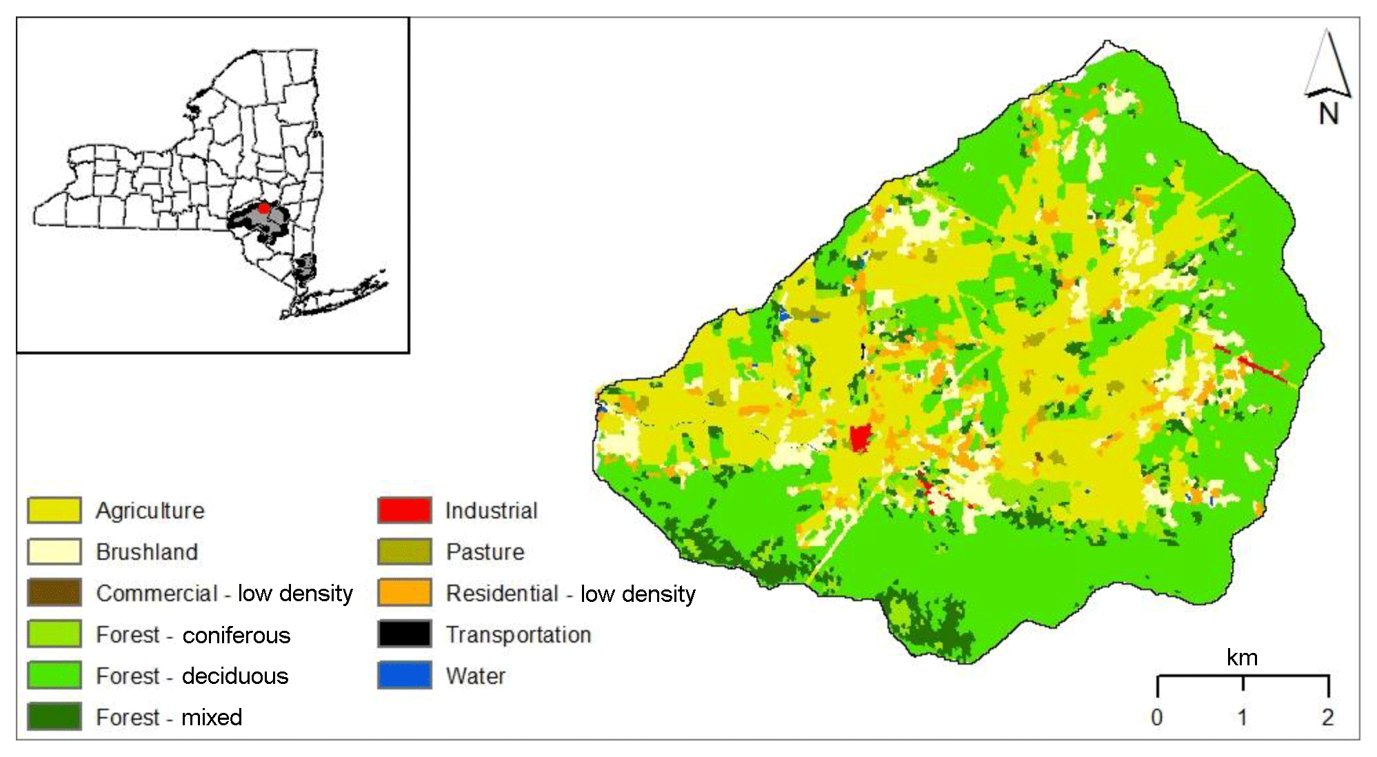
The 37 km2 Town Brook watershed is located in the Catskill Mountains, Delaware County, New York State (Fig. 1), and is the headwater of the Cannonsville Reservoir watershed, which is one of four reservoir watersheds in New York City's Delaware system. Elevation ranges from 493 to 989 m. The area is humid with an average temperature of 8 ∘C and average annual precipitation of 1123 mm yr−1. Approximately one-third of the total precipitation in the region falls as snow (Pradhanang et al., 2011). Most soils are either silt loam or silty clay loam. The upper terrain of the watershed has shallow soils (average thickness: 80 cm) overlaying fractured bedrock and steep slopes (average slope: 29 %), while deeper soils (average thickness: 180 cm) underlain by a dense fragipan-restricting layer and gentler slope (average slope: 14 %) are common in the lower terrain. Deciduous and mixed forests predominate in the upper terrain, covering more than half of the land area. In the lowland area, the principle land uses are agriculture (32 %), which includes dairy and beef farms with cropland and pastures; brushland (9 %); and residential areas (4 %).
2.2 Brief description of SWAT-HS
SWAT-HS is a modified version of the SWAT model version 2012 (SWAT2012) that is capable of predicting saturation-excess runoff. Two main modifications made in SWAT-HS include (i) adding information on topography and soil water storage capacity to the modeling unit of SWAT, i.e., hydrological response unit (HRU), and (ii) introducing a surface aquifer that allows lateral exchange of subsurface water from upslope to downslope areas.
Similar to SWAT, SWAT-HS divides the watershed into sub-basins. Additionally, the watershed is divided into a maximum of 10 wetness classes, each of which consists of areas in the sub-basin with similar topographic indices. Subsequently, the sub-basin is further divided into HRUs that are unique combinations of soil, land use and slope as in SWAT, with an additional component: wetness class. The topographic index (TI) is defined as
where TI is the soil topographic index (with units of ln; day m−1), α is the upslope contributing area per unit contour length (m), tan(β) is the local surface topographic slope, Ks is the mean saturated hydraulic conductivity of the soil (m day−1) and D is the soil depth (m).
The soil water storage capacity of the wetness classes is defined as the amount of water in the root zone between field capacity and saturation. This was assumed to vary across the soil wetness classes following a Pareto distribution (Hoang et al., 2017). Wetness classes that are located in the downslope areas have lower storage capacities, which means they are “wetter” than wetness classes in the upslope areas with smaller TI values and higher storage capacities. The wetter the wetness class, the faster the runoff response is during a rainstorm.
A surface aquifer is introduced to connect all wetness classes across the hillslope and transmits subsurface flow that is generated from this aquifer (known as lateral flow in SWAT) laterally through the hillslope from “drier” (upslope) to “wetter” (downslope) wetness classes.
SWAT-HS removes the original curve number method of SWAT in predicting total surface runoff. Instead, it simulates infiltration-excess runoff and saturation-excess runoff separately with different methods. Infiltration-excess runoff is predicted using the Green–Ampt method built into SWAT. Saturation-excess runoff in SWAT-HS is generated in the wetter (downslope) wetness classes by two processes: (i) rain falls in wet areas with limited storage capacities where the excess water becomes runoff, and (ii) water from the upland areas is transported laterally to the lowland areas and the water exceeding soil storage capacity becomes runoff (see Supplement for more details).
2.3 Methodology
2.3.1 Effect of DEM resolution
Four DEMs from fine to coarse resolution were used to set up the SWAT-HS model for the Town Brook watershed. The resolutions employed were 1, 3, 10 and 30 m. The 1 m DEM (DEM1m) was derived from 2009 aerial lidar data acquired by the New York City Department of Environmental Protection (RACNE, 2011). This was resampled to create 3, 10 and 30 m resolution DEMs (DEM3m, DEM10m and DEM30m).
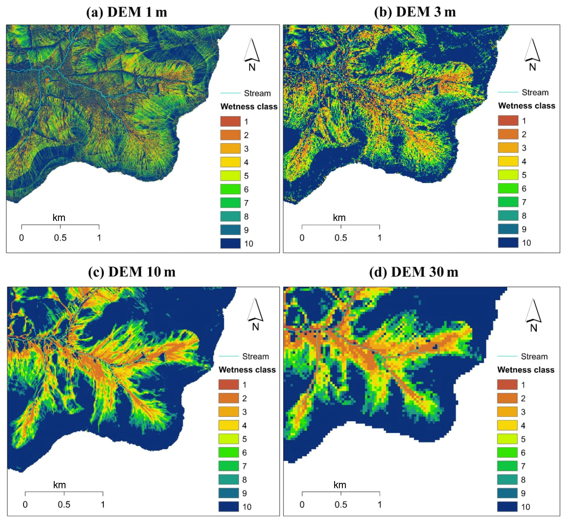
DEMs were used to delineate the watershed; calculate flow paths, slopes and drainage areas; and compute gridded values of TI. Based on TI values, the watershed was divided into 10 wetness classes (Fig. 4). Wetness class 1, covering a very small fraction of the watershed (0.59 %), corresponds to the perennial stream network and is the wettest wetness class. We grouped 50 % of the watershed with the lowest TI values in the upland as the “driest” wetness class (wetness 10), because saturated areas never exceeded 50 % of the watershed based on observations (Harpold et al., 2010) and predictions by other watershed models like the Soil Moisture Routing model (Agnew et al., 2006), SWAT-VSA (Easton et al., 2008) and SWAT-WB (White et al., 2011). Subsequently, we divided the remaining areas into eight wetness classes (wetness class 2–9) with approximately equal areas (∼6 % each) based on TI values. Applying the same procedure of wetness class division using four DEM resolutions, the four SWAT-HS setups have a relatively similar areal percentage of each wetness class.
HRUs were created based on 10 wetness classes, 17 soil types and 11 land use types. A single time series of daily precipitation and temperature data were interpolated from a 4 km × 4 km gridded PRISM climate data set (Daly et al., 2008) using the inverse distance weighting method. Solar radiation data were derived as the average of airport stations at Albany and Binghamton supplied by the Northeast Regional Climate Center. Relative humidity and wind speed were generated by the built-in weather generator in SWAT. The procedure outlined above is similar to the SWAT-HS setup used by Hoang et al. (2017).
Four SWAT-HS setups were run on a daily time step from 1998 to 2012. The first 3 years were used as the warming-up period, and the model was calibrated and validated for the periods 2001–2007 and 2008–2012, respectively. We excluded the year 2011 from the validation period because there were two extreme events (Hurricane Irene and Tropical Storm Lee) in August and September 2011 that the model could not capture well. The calibration was carried out in two stages, i.e., snowmelt calibration and flow calibration, and by applying the Monte Carlo sampling method. Since the Town Brook watershed is located in a region that is heavily impacted by snow, the prediction of snow storage and snowmelt will significantly affect the timing and volume of predicted streamflow in winter and early spring. Consequently, we divided the calibration in two stages in order to reduce the number of calibrated parameters involved in one calibration and to focus on getting the right results for snow processes before adjusting other processes.
For snowmelt calibration, we calibrated five snowmelt-related parameters in group (i) (Table 1) by generating randomly 10 000 parameter sets, running these sets using SWAT-HS, comparing the streamflow predictions with observations and choosing the best parameter set with the best fit to streamflow observations (highest value of daily Nash–Sutcliffe efficiency – NSE) to use for the flow calibration stage. For flow calibration, 10 000 parameter sets of nine flow parameters in group (ii) (Table 1) were generated which were then run with SWAT-HS. The simulations in the flow calibration stage were used for uncertainty analysis.
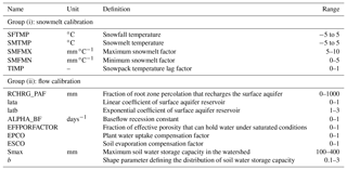
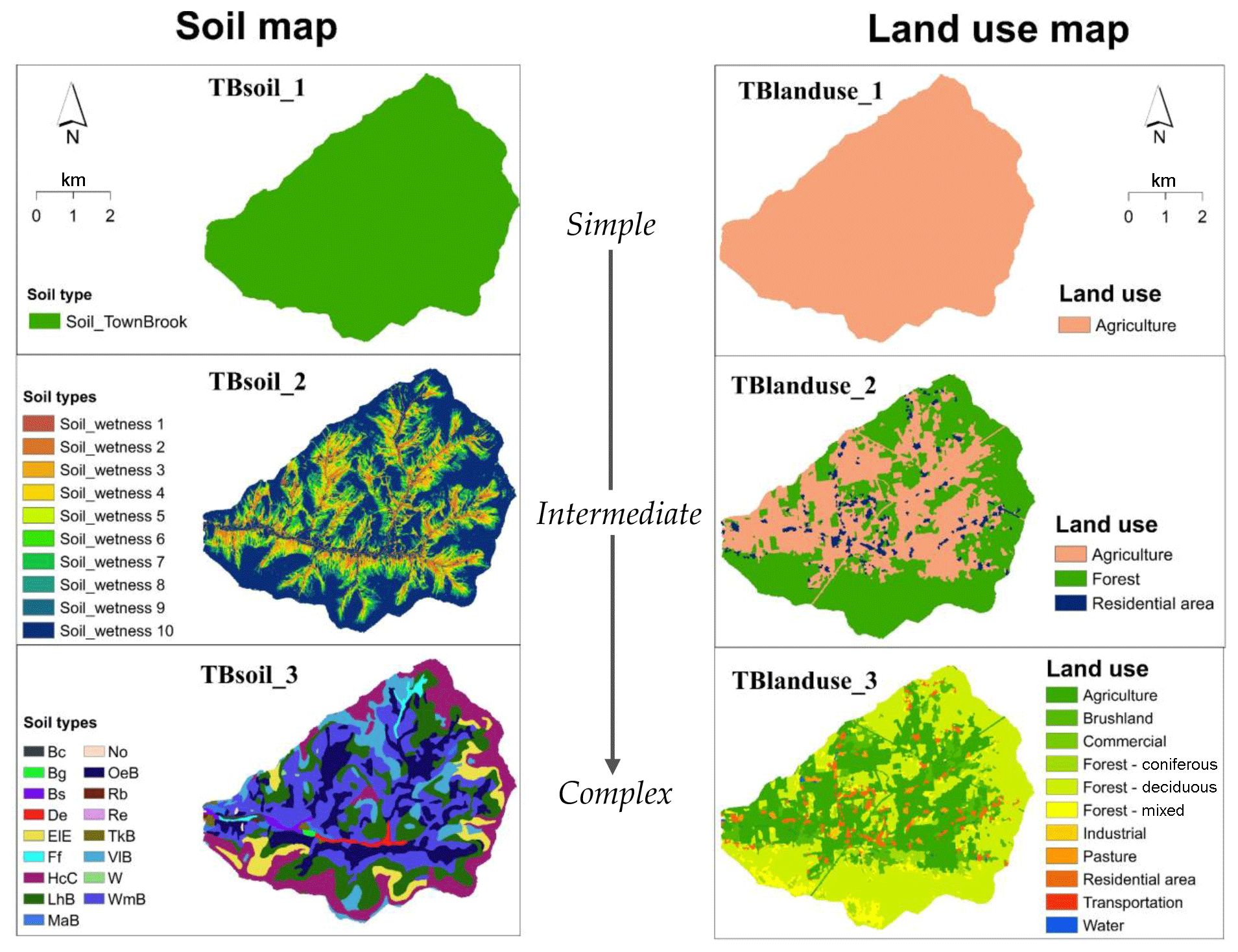
Figure 2Soil and land use maps with increasing levels of complexity to build SWAT-HS model setups.
We evaluated the effect of DEM resolution on representing topographical characteristics of the watershed by comparing the statistical distributions of elevation, slope angle, upslope contributing area and TI using DEMs with various spatial resolutions (1, 3, 10 and 30 m). Subsequently, to evaluate the effect of DEM resolution on model uncertainty, we compared the four SWAT-HS setups with different DEM resolutions based on (i) the uncertainty in streamflow predictions using “good”-performance parameter sets, (ii) predictions of saturated areas and their uncertainties, and (iii) uncertainty in parameter estimation. We used the generalized likelihood uncertainty estimation (GLUE) approach (Beven and Binley, 1992) to estimate the uncertainty in streamflow and saturated-area predictions caused by parameter uncertainty. For each model setup, good simulations were identified as those with a NSE greater than 0.65 for use in uncertainty estimation of streamflow. Our choice of NSE threshold at 0.65 is based on the guideline for model performance evaluation by Moriasi et al. (2007) that suggested good model performance for streamflow as corresponding to monthly NSE higher than 0.65. As NSE values at the monthly time step are usually higher than the daily values, we believe that our choice of NSE higher than 0.65 as good model performance for a daily time step is a reasonable choice. Subsequently, from these good simulations, we compared predictions of saturated areas with our available field observations of saturated areas to re-select the good parameter sets for both simulated streamflow and saturated areas, to estimate the uncertainty in predicted saturated areas. Six observations of saturated areas (28–30 April 2006, 12 April 2007, 7 June 2007 and 2 August 2007) are available for small areas in the headwaters of the Town Brook watershed.
2.3.2 Effect of soil and land use complexity
We built nine SWAT-HS setups ranging from simple (fewer soil types/land use classes, fewer HRUs) to complex (more soil types/land use classes, more HRUs) based on three soil maps and three land use maps. In all nine setups, DEM10m was used based on its performance as the best predictor of saturated areas (see discussion).
Three soil maps were created with increasing levels of complexity (Fig. 2). The simplest map (TBsoil_1) had a homogenous soil type, which was created using area-weighted average soil data from the four dominant soil types (Hcc, LhB, OeB, WmB) in Town Brook. The second soil map (TBsoil_2) had a unique soil type for each wetness class and was created by area-weighted averaging of dominant soil properties in the corresponding wetness class. The most complex soil map TBsoil_3 consisted of all 17 soil types.
Three land use maps with increasing levels of complexity were created (Fig. 2). The simplest land use map (TBlanduse_1) had agriculture as the representative land use for the watershed because it is one of the dominant land uses and potentially has a more significant impact on water quality than other land use types. The more complex land use map (TBlanduse_2) classifies Town Brook into three diverse land use types: agriculture, forest and urban areas. The most complex one (TBlanduse_3) contains all 11 land use types.
HRUs were generated based on a wetness map (10 classes), soil map, land use and slope maps. We assumed that slope does not have an impact on HRU discretization to simplify the setup. We also set a threshold of 1 % for soil and 1 % for land use to eliminate minor soil types/land uses that cover only less than 1 % of the sub-basin area.

Figure 3Difference in cumulative probability distribution of elevation, slope, upslope contributing area and topographic index between different DEM resolutions.
The nine model setups are categorized in three groups: (i) simple: the setups that use either the simplest soil or land use (TB1–TB5), (ii) intermediate: the setups that use the average complexity for maps of either soil or land use (TB6–TB8); and (iii) complex: the setup that uses the most complex maps (TB9) (Table 2).
To evaluate the effect of soil and land use data complexity on model uncertainty, we compared the nine SWAT-HS setups using the same methodology used to evaluate the effect of DEM resolution on model uncertainty that is described above.
Table 2SWAT-HS model setups with increasing levels of complexity.
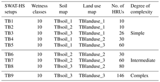
TBsoil_1: homogeneous soil; TBsoil_2: 10 soil types (unique soil type for each wetness class); TBsoil_3: 17 soil types; TBlanduse_1: homogenous land use (agriculture); TBlanduse_2: 3 land use types (agriculture, forest and urban); TBlanduse_3: 11 land use types.
3.1 The effect of DEM resolution on model uncertainty
3.1.1 Effect on topographic characteristics
DEM resolution has varying effects on the distribution of elevation, slope angle, upslope contributing area and TI values. However, the distributions of elevation are similar using different DEMs, indicating no effect from DEM resolution (Fig. 3a). The finer-resolution DEMs (DEM1m and DEM3m) are able to give more precise slope values. Therefore, coarser DEM resolutions produce slightly narrower slope distributions, lower mean slope angles, lower probability for steep slopes and higher probability for gentle slopes than the finer DEM resolutions because of the smoothing of topography and loss of topographic details (Fig. 3b). DEM resolution has a significant effect on the calculated values of upslope contributing areas (Fig. 3c). With the finer spatial resolutions, grids in DEM1m and DEM3m have smaller contributing areas than the ones in coarser-resolution DEM10m and DEM30m. This results in substantial differences in the distribution of TI in that the finer-resolution DEMs provide lower values of TI (Fig. 3d). The impact of DEM grid size on TI distribution is mainly due to its impact on upslope contributing area rather than slope. Our results are consistent with previous studies on the effect of DEM resolution on topographic attributes and topographic wetness index (Zhang and Montgomery, 1994; Thompson et al., 2001; Sørensen and Seibert, 2007; Gillin et al., 2015).
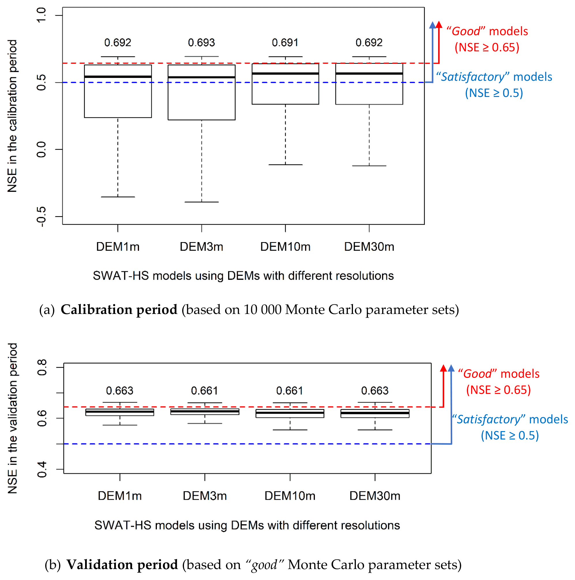
Figure 5Box plots of NSE values in SWAT-HS setups with different DEM resolutions for calibration and validation periods (the number above the box plot is the maximum NSE of each setup).
Depending on the DEM used, the four wetness maps formed by grouping areas of similar TI into 10 wetness classes show remarkable differences (Fig. 4). It should be noted here that the differences are in the spatial distribution of wetness classes, while the areal percentage of each wetness class is relatively similar irrespective of the DEM used. In Fig. 4, we show the wetness maps for the headwater area where observations of saturated areas are available. It can be clearly seen that the spatial patterns of wetness classes in coarser-resolution DEMs (10 and 30 m) are quite similar but are very different from the finer-resolution DEMs (1 and 3 m). DEM1m has a complex pattern with all wetness classes spread out, making it difficult to see their boundaries, while the pattern becomes more coherent in coarser DEMs where the boundaries of the wetness classes are easier to distinguish. Our results are consistent with previous studies on the effect of grid size on spatial patterns of topographic wetness index that have been reported by Thomas et al. (2017), Erskine et al. (2006), and Zhang and Montgomery (1994).
3.1.2 Effect on the prediction of streamflow
To evaluate the effect of DEM on the uncertainty of streamflow predictions, we compared streamflow outputs from 10 000 Monte Carlo simulations of four model setups with DEMs of different resolutions (Fig. 5a). Subsequently, we evaluated and compared streamflow estimates in the validation period based on only good parameter sets (Fig. 5b). Statistical criteria for evaluating uncertainty are shown in Table 3. The comparison between observed flow and 90 % prediction uncertainty measured between the 5th and 95th percentiles of predicted flows from good parameter sets is shown in Fig. S3 in the Supplement. In all setups, more than 50 % of the parameter sets give “satisfactory” performances (NSE ≥ 0.5) (Fig. 5). Of the total randomly generated parameter sets, 14 %–23 % give good streamflow performance in the four setups, with higher percentages in coarser-resolution setups (DEM10m and DEM30m) (Table 3). For the calibration period, the maximum NSE, NSElog and Kling–Gupta efficiency (KGE) values are equivalent (around 0.69, 0.82 and 0.81, respectively) in the four setups. However, the median NSE, mean NSE, mean NSElog and mean KGE are all higher in coarser-resolution setups (DEM10m and DEM30m) than the higher-resolution ones (DEM1m and DEM3m). In the finer-resolution setups, there are higher percentages of parameter setups that give poor fit to observed streamflow (NSE is negative), which causes lower mean values of NSE as well as NSElog and KGE. The uncertainty ranges of predicted flows, particularly intermediate flows, are wider in the finer-resolution setups (Fig. S3), although uncertainty bounds match observations very well in all four setups. For the validation period, the good parameter sets all give above-satisfactory to good fit to observations and relatively similar performance to each other. Generally, there are only slight differences in SWAT-HS performance on streamflow using different DEMs, implying the insignificant effect of DEM resolution on streamflow simulation and the uncertainty of streamflow outputs.
Table 3Statistical criteria to compare the effect of DEM resolution on model uncertainty.
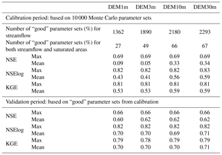
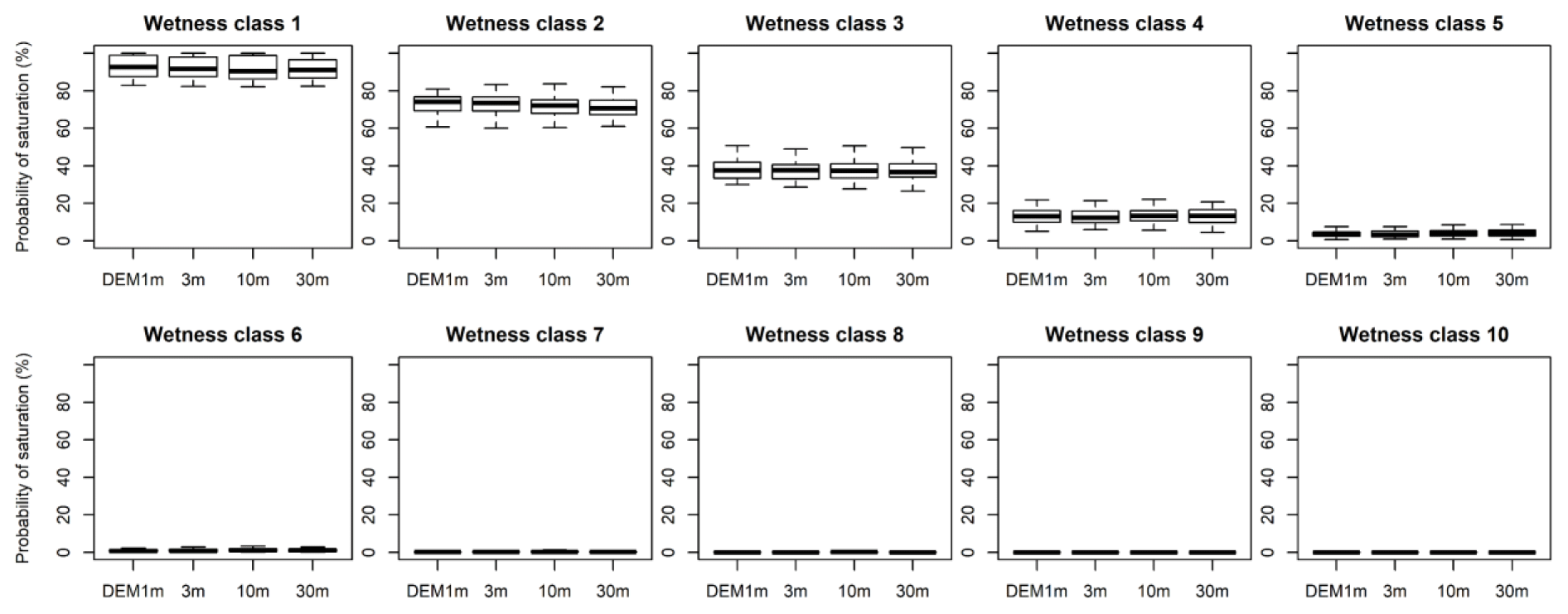
Figure 6Probability of saturation of wetness classes in SWAT-HS setups with different DEM resolutions using good parameters for both streamflow and saturated areas.
Although the effect of DEMs on streamflow prediction is minor, the setups using coarser-resolution DEM10m and DEM30m are slightly better and preferred for application. These two setups give higher NSE value ranges, and significantly higher mean NSE values resulted from all random combinations of parameters than the finer-resolution setups. These two setups also have more good parameter sets, indicating a higher probability of getting good representation of the modeled watershed. This implies better streamflow prediction by these two setups even without calibration.
3.1.3 Effect on the prediction of saturated areas
The probabilities of saturation in 10 wetness classes were compared among four DEM resolution setups using only good parameter sets for both streamflow and saturated-area predictions (Fig. 6). The probability of saturation, which indicates the number of days in the calibration period when the wetness class is saturated, shows no significant difference among the four setups, indicating that DEM resolution does not have an impact on the probability of saturation. It is important to note that we tried to keep the areal percentage of each wetness class approximately the same in the four setups using different DEMs. The good parameter sets in four setups should give comparable predictions of overall streamflow, percentage of watershed area that is saturated and the time that each wetness class was saturated, which results in similar probability of saturation. Wetness classes 7 to 10 are predicted to be mostly dry, implying that almost 70 % of the watershed is rarely saturated. Wetness class 1 has a high probability of saturation (80 %–100 %) because its soil water storage capacity is very low; i.e., the wetness class is prone to saturation whenever there is precipitation. The probability of saturation decreases in the more upslope wetness classes: 60 %–80 % in wetness class 2, 30 %–50 % in class 3, 5 %–22 % in class 4, 1 %–9 % in class 5, 0 %–3 % in class 6, 0 %–1 % in class 7, 0 %–0.3 % in class 8, 0 %–0.08 % in class 9 and 0 % in class 10. We also observed that the uncertainty of saturation probability of the more upslope wetness classes is lower because they only respond to high-rainfall events.
The results of the probability of saturation correspond well with the uncertainty of percentage of saturated areas shown in Fig. 7. The four model setups do not have significant differences in the percentage of saturated areas in the watershed. The maximum, minimum and interquartile range indicated by the top and bottom values of the four box plots are slightly different because of minor differences in division of wetness classes in the watershed. For the majority of the time, no more than approximately 25 % of the total watershed area is saturated. The watershed can be saturated up to more than 50 % in extreme events that are shown as outliers in the box plots. The median percentage of saturated areas in the watershed is only around 7 %–8 %.
Although the statistical distributions of saturated areas in four DEM setups are relatively similar, the spatial distributions of saturated areas simulated in a small headwater area (Fig. 1) on specific days (28–30 April 2006), when observations are available, appeared to be different as shown in Fig. 8. In Fig. 8, the saturated areas simulated in four DEM setups correspond to the saturation of wetness classes 1–3. Saturated areas cover approximately equal areas of the watershed for the different DEM resolutions but differ significantly in spatial distribution. The saturated areas resulting from DEM1m and DEM3m are scattered, not well connected and broadly distributed. For coarser-resolution DEM10m and DEM30m, saturated areas connect well with each other and with the areas concentrated near streams. The percentages of simulated saturated areas that intersect with observations increase with coarser-resolution DEMs: 34 % (DEM1m), 53 % (DEM3m), 85 % (DEM10m) and 90 % (DEM30m). Therefore, based on visual comparison with observations and our calculation, the coarser-resolution DEMs give better fits to observed saturated areas than the higher-resolution DEMs. Among the four DEMs, DEM10m provides the most realistic representation of saturated areas and reasonable fit to observations.
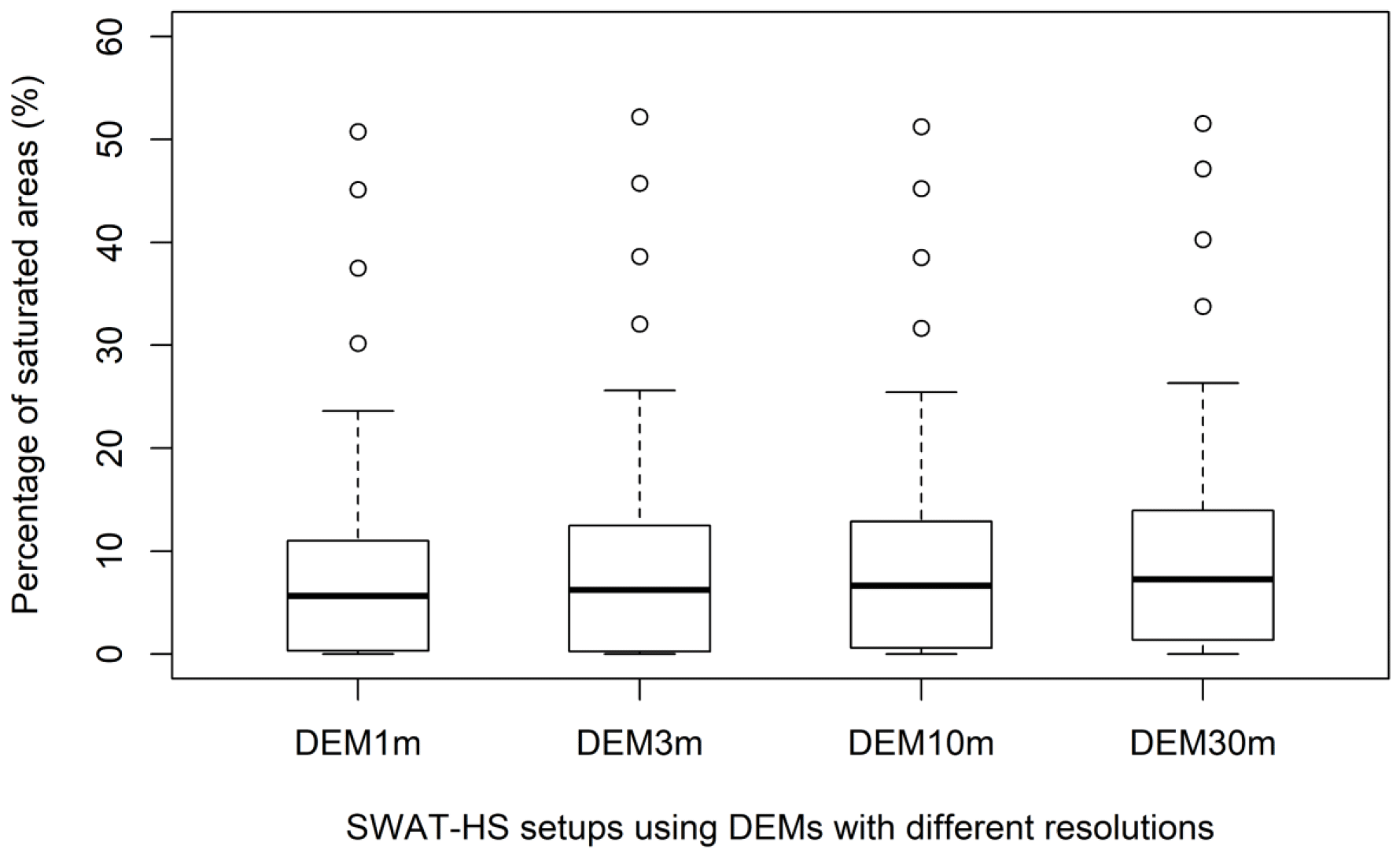
Figure 7Percentage of saturated areas taking into account parameter uncertainty in the calibration period in SWAT-HS setups using DEMs with different resolutions.
3.1.4 Effect on parameter uncertainty
Figure 9 shows the comparison between the distribution of good parameters for streamflow (in green) and the distribution of good parameters for both streamflow and saturated areas (in blue) in four SWAT-HS model setups with different-resolution DEMs. Only two parameter distributions (latb and Smax) are plotted in Fig. 9 because they are the most sensitive parameters (Hoang et al., 2017). Although the number of good parameters for streamflow varies in four setups, the ranges of good parameter values and the shape of their distributions are alike for all calibrated parameters. Using multiple observations (both streamflow and saturated areas) helps to reduce a great number of good parameters in all four setups but does not significantly narrow down the value ranges of good parameters. The similarity in the distribution of good parameters in four setups with different DEM resolutions implies that DEM resolution has a negligible impact on parameter uncertainty for this watershed.
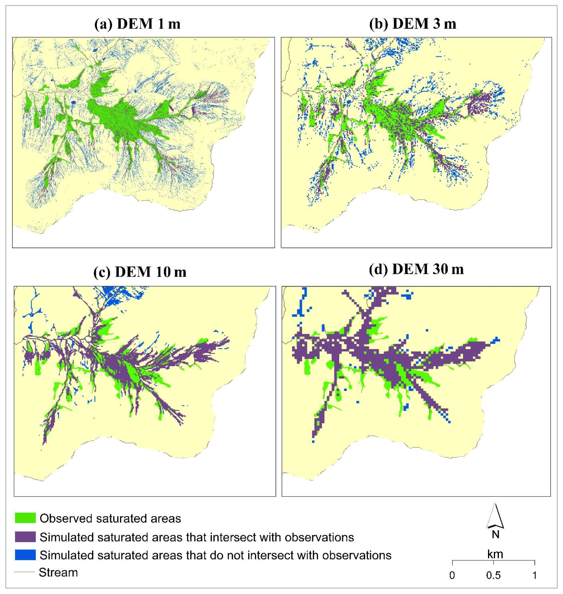
Figure 8Simulated and observed saturated areas from four SWAT-HS setups using different DEMs, 28–30 April 2006.
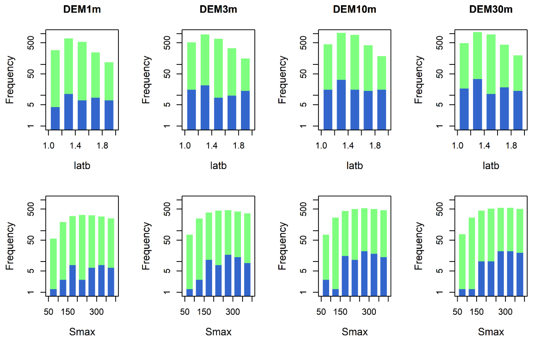
Figure 9Distribution of good parameters for streamflow (in green) and for both streamflow and saturated areas (in blue) with log y axis in four SWAT-HS setups using different DEM resolutions.
Table 4Statistical criteria to compare the effect of input complexity on model uncertainty.
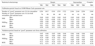
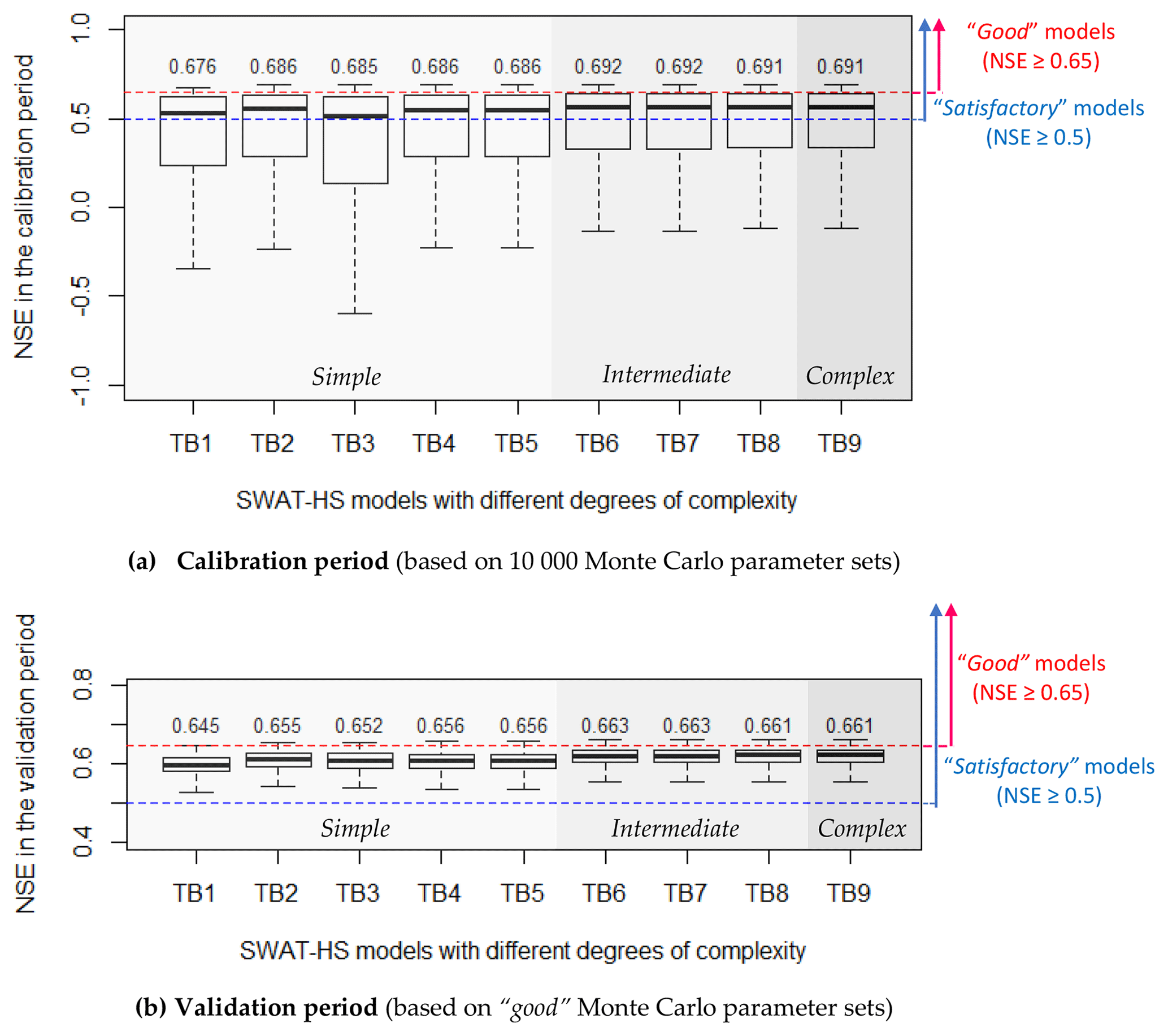
Figure 10Box plots of NSE values in SWAT-HS setups with different degrees of complexity for calibration and validation periods (the number above the box plot is the maximum NSE of each setup).

Figure 11Distribution of good parameter values (parameter latb) for streamflow (in green) and for both streamflow and saturated areas (in blue) with log y axis in nine SWAT-HS setups with different degrees of complexity.
3.2 Effect of soil and land use input complexity on model uncertainty
3.2.1 Effect on uncertainty in streamflow predictions
All nine SWAT-HS setups with different degrees of complexity are able to obtain good model performance and are comparable to one another (Fig. 10 and Table 4). More than 50 % of the total simulations in each setup produce NSE greater than 0.5, which corresponds to satisfactory performance. All setups also have high percentages of good performance (12.5 %–22.6 %), with TB1 and TB8 having the lowest and highest percentages, respectively. The maximum NSE, NSElog and KGE obtained from nine setups are relatively equivalent. The mean values of the three metrics are slightly different, except for the TB3 setup, with the lowest mean values in all three metrics. This is also reflected in Fig. S4, showing that all setups capture measured streamflow well within their uncertainty ranges, with TB3 being the poorest setup with the widest uncertainty range. Applying only the good parameter sets in the validation period, we observe insignificant differences among the nine setups, but TB3 still performs the worst in low flow with the lowest NSElog. All these good parameter sets give above-satisfactory to good fit to observations in the validation periods, implying that all nine setups are reasonable to use for flow predictions. In spite of minor differences, from all the evaluation criteria, TB3 gives the poorest performance among nine setups, followed by the simplest setup: TB1. Setups TB6 to TB9 give equally good performance and are better than the remaining ones.
Grouping the nine setups into three groups – (i) simple (TB1–TB5), (2) intermediate (TB6–TB8) and (iii) complex (TB9) – we observe that the model performance of setups in intermediate groups are slightly better than the simple one, although the differences are small. The intermediate group has a higher number of good parameter sets, a higher mean NSE in the calibration period and consistently better performance in the validation period. The most complex setup (TB9) gives equally good performance to setups in the intermediate group with no improvement in any statistical metric.
All nine setups use the same DEM with 10 m resolution and have the same distribution of wetness classes; therefore, the distributions of their predicted saturated areas are similar and thus are not shown here.
3.2.2 Effect on parameter uncertainty
We tested the effect of soil and land use complexity on parameter uncertainty by comparing the distribution of good parameters among nine setups with different degrees of complexity, as in Fig. 11. We only showed the distribution of one calibrated parameter (latb) as an example because we observed the same behavior in the remaining calibrated parameters. Similar to the comparison of four setups using different DEMs, the nine setups with different degrees of complexity produce different numbers of good parameters for streamflow and saturated areas but are similar in the shape of their distributions and value ranges. Accordingly, soil and land use complexity have negligible effects on parameter uncertainty.
The objective of this study is to estimate uncertainty in model parameterization, and predictions of streamflow and saturated areas due to the effects of DEM resolution and complexity in model setup, specifically combinations of land use and soils. The following sections discuss the proposed research questions based on the results obtained.
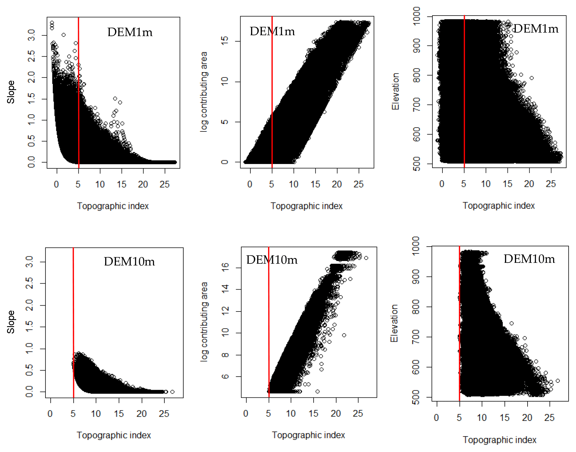
Figure 12Relationships of topographic index with slope, upslope contributing area and elevation with two different DEM resolutions: 1 and 10 m (red lines are used as reference to compare the two DEM resolutions).
4.1 What is the most suitable DEM resolution to use in SWAT-HS?
Our results show that randomly generated parameter values from coarser-resolution DEMs (DEM10m and DEM30m) perform better for streamflow prediction. However, after calibration, the effect of DEM resolution on the uncertainty of streamflow prediction is very minor. This result is in agreement with Liu et al. (2005) using the WetSpa model with 50–800 m cell sizes, Molnar and Julien (2000) using the CASC2D model with 127–914 m cell sizes and Chaplot (2005) using SWAT with 20–500 m DEMs. These studies found that discharge was simulated equally well irrespective of DEM resolution as long as parameters were calibrated properly.
DEM resolution has very limited impact on probability of saturation in wetness classes and percentage of saturated areas in the watershed but greatly influences the spatial distribution of saturated areas. SWAT-HS simulates the saturation-excess runoff coming from saturated areas based on a statistical soil water distribution assigned to wetness classes. The wettest wetness classes downslope with lowest soil water storage capacity are saturated first followed by drier adjacent wetness classes located more upslope. Therefore, the distribution of saturated areas follows the distribution of wetness classes categorized by the values of TI. Accordingly, the sensitivity of DEMs on saturated-area predictions can be explained by the effect of DEM resolution on TI.
Figure 12 shows the relationships of TI with slope angle, upslope contributing area and elevation using two representative DEM resolutions: 1 and 10 m. It is evident that DEM1m can capture a significantly wider range of slopes than DEM10m because of its finer resolution. Also, the percentage of grids that have low values of TI is significantly higher in DEM1m than in DEM10m (Fig. 12 uses red lines for reference), which also can be seen in Fig. 3d. Low TI values are usually found in grids with steep slopes or with low upslope contributing areas (according to Eq. 1). Because DEM1m captures steep slopes at a local scale and has a high number of grids with low upslope contributing area (Fig. 3c), the percentage of low TI values in DEM1m is much higher. If we look at the relationship between TI and elevation, we can see that the distribution of TI values in DEM1m spread out wider than in DEM10m at all elevations. This explains why the distribution of TI values in DEM1m has a more complex pattern while DEM10m has a more coherent pattern with high TI grids well matched to the stream network (Fig. 13). Because of that, in this case study, the coarser DEMs (DEM10m and 30 m) give a more suitable representation of the landscape than the finer DEMs (DEM1m and 3 m). This is possibly the reason why the coarser DEM setups have higher probabilities for good performance (i.e., a higher number of good parameter sets) and have better performance in all aspects as compared with the finer DEMs.

Our findings are in agreement with Lane et al. (2004), who used a 2 m high-resolution lidar DEM with TOPMODEL (TOPography-based hydrological MODEL), which simulates hydrology based on TI. TOPMODEL predicted the widespread existence of disconnected saturated zones that expanded within an individual storm event but which did not necessarily connect with the drainage network. They found that, when using the lidar DEM 2 m, TI has a complex pattern, associated with small areas of both low and high values of the TI, leading to the appearance of disconnected saturated areas. After remapping the topographic data at progressively coarser resolutions by spatial averaging of elevations within each cell, they found that, as the topographic resolution was coarsened, the number and extent of unconnected saturated areas were reduced, and the catchments displayed more coherent patterns, with saturated areas more effectively connected to the channel network. Moreover, Quinn et al. (1995) showed how progressively refining model resolution from 50 to 5 m reduces the kurtosis in the distribution of TI values and increases quite substantially the number of very low index values.
For the Town Brook watershed, DEM10m is the best choice among four DEMs tested because of its slightly better performance for streamflow and, more importantly, its good fit to observations of saturated areas. Although DEM30m also gives very good results for streamflow and distribution of saturated areas, we did not choose DEM30m because its coarse cell size may overestimate the extent of actual saturated areas. Therefore, DEM10m is the preferred choice for scaling up the application of SWAT-HS to larger watersheds in the New York City water supply system for future applications. Our choice of DEM10m is in agreement with Kuo et al. (1999), who evaluated the effect of DEM grid sizes ranging from 10 to 400 m on runoff and soil moisture for a variable-source-area hydrology model and observed that when using the 10 m × 10 m grid cells the overall pattern of simulated wet areas showed a close correspondence with the poorly drained areas defined in the soil survey. Zhang and Montgomery (1994), in a study that evaluated grid size effect using TOPMODEL, also suggested that a 10 m grid size presents a rational compromise between increasing resolution and data volume for simulating geomorphic and hydrological processes. In contrast, Thomas et al. (2017) indicated that lidar DEM 1–2 m is optimal for modeling hydrologically sensitive (runoff-generating) areas and is far better than the radar-based DEM5m. However, their case study is a complex agricultural catchment dominated by micro-topographic features, which can only be captured using high-resolution DEMs. Our choice of DEM10m is in contrast to Buchanan et al. (2014), who preferred DEM3m rather than DEM10m because of the better fit with the observed patterns of soil moisture collected at five different agricultural field sites. The difference in scale of case studies (field scale vs. watershed scale) and characteristics of case studies (agricultural fields vs. a mixture of forest and agriculture) between Buchanan et al. (2014) and our study may have resulted in different conclusions on choice of the appropriate DEM resolution. Therefore, the sensitivity of DEM resolution may depend on the scale and characteristics of the watershed. The dominant hydrological process in the watershed may have a big impact on the sensitivity of DEM on hydrological prediction. In the Town Brook watershed, lateral flow is a dominant flow component and saturation-excess runoff is a dominant type of surface runoff; thus, topography is the most important factor. Consequently, DEM10m that represents a realistic distribution of TI, with high-TI area compatible with the main stream network, gave a better model performance. In a field-scale watershed, finer DEM resolution is probably better because it can capture a more detailed and realistic representation of TI distribution. In an agricultural area dominated by subsurface tile drainage, DEM resolution may not be sensitive.
It should be noted here that all four DEMs in this study are derived from the same source of 2009 aerial lidar data with 1 m resolution. The coarser DEMs (DEM3m, DEM10m and DEM30m) are resampled products from DEM1m. Therefore, the four different DEM resolutions carry similar information but differ in topographic smoothing. A comparison of various-resolution DEMs from different sources may not yield the same results.
4.2 What is the appropriate complexity of the distributed soil and land use inputs?
From our comparison of nine SWAT-HS setups in three groups of complexity (simple, intermediate and complex), we found that with all randomly generated parameter values the intermediate and complex groups are better than the simple group based on slightly higher mean NSE values and a higher probability of good performance based on randomly generated parameter values. The TB3 setup, which was built from the most complex soil map (17 soil types) and the simplest land use map (1 land use) and the simplest setup TB1 are the two poorest setups in the simple group. Additionally, compared to the intermediate group, the complex group does not gain any improvement from using inputs that are more detailed. However, with proper calibration, all nine models are able to provide good performances, and their good parameter sets continue to perform equally well in the validation period. In addition to streamflow, all nine setups are able to capture saturated areas correctly on specific days where observations are available. We conclude that increasing spatial input details does not necessarily give better results for streamflow simulation as long as the model is properly calibrated. However, oversimplification like the simple setups TB1 and TB3 with only one land use type may have greater impacts on water quality modeling. We recommend using intermediate inputs for the SWAT-HS setup that adequately represent the spatial distribution of dominant soils and land use types.
Our results are in agreement with previous studies on the effect of model input complexity on streamflow simulation. Using an urban hydrological distributed model in a small residential area, Petrucci and Bonhomme (2014) showed that the inclusion of some basic geographical information that helps to correctly estimate impervious cover and identify paths for surface water improves the model performance, but further refinements are less effective. Finger et al. (2015) compared different setups with increasing detail in input information using the HBV model and three observational data sets. They found that enhanced model input complexity does not lead to a significant increase in overall performance in water quantity, but they suggested that the availability and use of different data sets to calibrate hydrological models might be more important than model input data complexity to achieve realistic estimations of runoff composition. Muleta et al. (2007) also showed that streamflow simulated by SWAT is relatively insensitive to spatial scale when comparing multiple watershed delineations from different soil and land use input data.
In comparison with the effect of DEM resolution, the importance of soil and land use information is not as significant in the prediction of both streamflow and saturated areas. As our studied watershed is a rural area and dominated by saturation-excess runoff, topography and the wetness conditions of areas in the watershed are more important than land use in water quantity modeling. Moreover, SWAT-HS uses TI as the basis for hydrological modeling; thus, the effect of DEM resolution on hydrological predictions is dominant. Therefore, when the appropriate DEM resolution is used, soil and land use information becomes less sensitive to hydrological predictions. We think that this finding is applicable to watersheds where application of SWAT-HS is suitable, i.e., watersheds dominated by saturation-excess runoff. This finding may be also valid in applications of other topography-based watershed models, including TOPMODEL (Beven and Kirkby, 1979; Quinn and Beven, 1993), SWAT-VSA (Easton et al., 2008) and SWAT-WB (White et al., 2011). These results may not be applicable in water quality modeling. Since land use information controls the inputs of nutrients and information of other human activities that affect water quality, the water quality prediction is expected to be very sensitive to the details of land use.
4.3 How does input complexity affect parameter uncertainty and model output uncertainty?
Our results show that, regardless of the level of detail of input data, we obtained numerous sets of parameter values that give equally good performance for streamflow and saturated-area predictions. Modifying the level of detail in input data changes the number of good parameter sets, but the ranges of good parameter values and the shape of their distributions remain the same. The number of randomly generated Monte Carlo parameter sets is sufficiently high to give a good coverage of parameter space. Although different inputs result in varied numbers of good parameter sets, those numbers in all setups are adequate to represent the distribution of good parameters, which reflects their sensitivities to hydrological prediction. Therefore, we conclude that for this case study and the particular model SWAT-HS using higher-resolution DEM or adding complex information on soil or land use does not reduce parameter uncertainty or solve the equifinality problem. This statement may not be valid for other areas that are characterized by numerous land uses and complex variations in topography and soil types. This is also not valid for physically based models which require detailed soil and land use information and a minimum number of parameters for calibration.
Combining different observations (temporal observations of streamflow and spatial observations of saturated areas on multiple days) in calibration will help to reduce the number of good parameter sets and choose the appropriate parameter sets that give good representation of hydrological processes in the watershed. The importance of using multiple data sets has been addressed in Finger et al. (2015), McMillan et al. (2011) and Kirchner (2006). Our study is not aimed at solving the equifinality problem but rather reduces the number of solutions considered when using SWAT-HS to predict streamflow. The outcome of this study directly reduces the decision uncertainty with regard to selecting the optimum combination of input data sets for model setup that gives the best model results both spatially and temporally. This has implications for watershed modeling by reducing model run time as we scale up the application of SWAT-HS to other larger watersheds within the NYC water supply system.
This paper is a follow-up to our previous study using the SWAT-HS model, investigating the effect of input data complexity on the uncertainty in predictions of streamflow and saturated areas. The input data include DEMs with different resolutions and different combinations of simple to complex soil and land use maps. The main objectives are to explore whether using more complex spatial data yields better, more robust results and to guide the selection of the most appropriate input data for future applications of SWAT-HS in other watersheds or larger watersheds within the New York City water supply system.
We chose DEM10m resampled from lidar DEM1m as the most appropriate resolution because DEM10m gives a better physical representation of the landscape and is a compromise between the high-resolution DEM1m and DEM3m that provide too much spatial detail, which affects the calculation of upslope contributing areas and TI, and coarse-resolution DEM30m that averages out the essential details. We recommend the use of an intermediate soil and land use map for our future applications of SWAT-HS. Our results show that streamflow is sensitive neither to DEM resolution nor to soil and land use complexity as long as proper calibration is carried out. However, DEM resolution has a significant impact on the spatial distribution of predicted saturated areas due to its substantial control on the distribution of TI values. The effect from soil and land use inputs becomes minor when the appropriate DEM resolution is used in the model setup.
For the New York City watershed region, our study will provide guidance for choosing input data (DEM resolution and the degree of complexity for soil and land use) to apply SWAT-HS in a larger-scale watershed that requires division into multiple sub-basins and a certain degree of complexity for soil and land use information. Our results are particularly informative when we use SWAT-HS to identify critical runoff-generating areas and locations within the watershed where management interventions for water quality improvements (e.g., phosphorus load reduction) are most effective. Besides New York City watersheds, our findings are applicable to watersheds with similar land use, topography and climate, but similar investigation is needed in other regions using the methodology described in this paper.
From this study it can be inferred that hydrological prediction is very sensitive to the choice of DEM (with greater effects on prediction of saturated areas than streamflow) when using a hydrologic model that uses topographic index as the basis for hydrological modeling in a watershed that is dominated by saturation-excess runoff. With SWAT-HS and models that are based on TI such as TOPMODEL, SWAT-VSA and SWAT-WB, DEM resolution is more influential than the complexity of soil/land use information. When the appropriate DEM resolution is used, soil and land use information becomes less influential in hydrological predictions.
Regardless of the level of detail for input data, the equifinality problem can cause uncertainty in modeled results when using different SWAT-HS setups. Increasing input data complexity does not help to reduce parameter uncertainty and the uncertainty of model predictions. However, using multiple types of observed data sets such as spatial observations in addition to the conventional temporal observations can eliminate a high number of unsuitable parameter sets and guide selection of the appropriate parameter sets that give good temporal and spatial predictions for streamflow and saturated areas.
The data used in this paper are not publicly accessible. However, the first author can be contacted by email for help in providing online sources to download some of the data and contacts to acquire other data.
The supplement related to this article is available online at: https://doi.org/10.5194/hess-22-5947-2018-supplement.
LH set up the models, performed analysis, wrote the paper and responded to the reviewers. RM contributed to performing analysis, writing the paper and responding to the reviewers. KEBM collated the data and contributed to writing and editing the paper. EMO contributed to writing and editing the paper. TSS initialized the idea for carrying out this study and contributed to writing and editing the paper.
The authors declare that they have no conflict of interest.
The authors thank Willem Vervoort and an anonymous referee for their constructive
comments and suggestions; the editor, Micha Werner, for smooth handling of the
review process; and the New York City Department of Environmental Protection (NYCDEP)
for providing data and financial support through a contract with the City University
of New York.
Edited by: Micha Werner
Reviewed by: Willem Vervoort and one anonymous referee
Agnew, L. J., Lyon, S., Gérard-Marchant, P., Collins, V. B., Lembo, A. J., Steenhuis, T. S., and Walter, M. T.: Identifying hydrologically sensitive areas: Bridging the gap between science and application, J. Environ. Manage., 78, 63–76, https://doi.org/10.1016/j.jenvman.2005.04.021, 2006.
Arnold, J. G., Srinivasan, R., Muttiah, R. S., and Williams, J. R.: Large area hydrologic modeling and assessment part 1: Model development, J. Am. Water Resour. Assoc., 34, 73–89, https://doi.org/10.1111/j.1752-1688.1998.tb05961.x, 1998.
Bárdossy, A. and Singh, S. K.: Robust estimation of hydrological model parameters, Hydrol. Earth Syst. Sci., 12, 1273–1283, https://doi.org/10.5194/hess-12-1273-2008, 2008.
Beck, M. B.: Water quality modeling: a review of the analysis of uncertainty, Water Resour. Res., 23, 1393–1442, https://doi.org/10.1029/WR023i008p01393 1987.
Beven, K. and Binley, A.: The future of distributed models: Model calibration and uncertainty prediction, Hydrol. Process., 6, 279–298, https://doi.org/10.1002/hyp.3360060305, 1992.
Beven, K. and Freer, J.: Equifinality, data assimilation, and uncertainty estimation in mechanistic modelling of complex environmental systems using the GLUE methodology, J. Hydrol., 249, 11–29, https://doi.org/10.1016/S0022-1694(01)00421-8, 2001.
Beven, K. J. and Kirkby, M. J.: A physically based, variable contributing area model of basin hydrology, Hydrolog. Sci. Bull., 24, 43–69, https://doi.org/10.1080/02626667909491834 1979.
Buchanan, B. P., Fleming, M., Schneider, R. L., Richards, B. K., Archibald, J., Qiu, Z., and Walter, M. T.: Evaluation topograpic wetness indices across central New York agricultural landscapes, Hydrol. Earth Syst. Sci., 18, 3279–3299, https://doi.org/10.5194/hess-18-3279-2014, 2014.
Chaplot, V.: Impact of DEM mesh size and soil map scale on SWAT runoff, sediment, and NO3–N loads predictions, J. Hydrol., 312, 207–222, https://doi.org/10.1016/j.jhydrol.2005.02.017, 2005.
Chaubey, I., Cotter, A., Costello, T., and Soerens, T.: Effect of DEM data resolution on SWAT output uncertainty, Hydrol. Process., 19, 621–628, https://doi.org/10.1002/hyp.5607, 2005.
Cibin, R., Sudheer, K., and Chaubey, I.: Sensitivity and identifiability of stream flow generation parameters of the SWAT model, Hydrol. Process., 24, 1133–1148, https://doi.org/10.1002/hyp.7568, 2010.
Cotter, A. S., Chaubey, I., Costello, T. A., Soerens, T. S., and Nelson, M. A.: Water quality model output uncertainty as affected by spatial resolution of input data, J. Am. Water Resour. Assoc., 39, 977–986, https://doi.org/10.1111/j.1752-1688.2003.tb04420.x, 2003.
Daly, C., Halbleib, M., Smith, J. I., Gibson, W. P., Doggett, M. K., Taylor, G. H., Curtis, J., and Pasteris, P. P.: Physiographically sensitive mapping of climatological temperature and precipitation across the conterminous United S tates, Int. J. Climatol., 28, 2031–2064, https://doi.org/10.1002/joc.1688 2008.
Easton, Z. M., Fuka, D. R., Walter, M. T., Cowan, D. M., Schneiderman, E. M., and Steenhuis, T. S.: Re-conceptualizing the soil and water assessment tool (SWAT) model to predict runoff from variable source areas, J. Hydrol., 348, 279–291, https://doi.org/10.1016/j.jhydrol.2007.10.008, 2008.
Erskine, R. H., Green, T. R., Ramirez, J. A., and MacDonald, L. H.: Comparison of grid-based algorithms for computing upslope contributing area, Water Resour. Res., 42, W09416, https://doi.org/10.1029/2005WR004648 2006.
Finger, D., Vis, M., Huss, M., and Seibert, J.: The value of multiple data set calibration versus model complexity for improving the performance of hydrological models in mountain catchments, Water Resour. Res., 51, 1939–1958, https://doi.org/10.1002/2014WR015712, 2015.
Geza, M. and McCray, J. E.: Effects of soil data resolution on SWAT model stream flow and water quality predictions, J. Environ. Manage., 88, 393–406, https://doi.org/10.1016/j.jenvman.2007.03.016, 2008.
Gillin, C. P., Bailey, S. W., McGuire, K. J., and Prisleyt, S. P.: Evaluation of LiDAR-derived DEMs through terrain analysis and field comparison, Photogram. Eng. Remote Sens., 81, 387–396, https://doi.org/10.14358/PERS.81.5.387, 2015.
Harpold, A. A., Lyon, S. W., Troch, P. A., and Steenhuis, T. S.: The hydrological effects of lateral preferential flow paths in a glaciated watershed in the Northeastern USA, Vadose Zone J., 9, 397–414, https://doi.org/10.2136/vzj2009.0107 2010.
Hoang, L., Schneiderman, E. M., Moore, K. E. B., Mukundan, R., Owens, E. M., and Steenhuis, T. S.: Predicting saturation-excess runoff distribution with a lumped hillslope model: SWAT-HS, Hydrol. Process., 31, 2226–2243, https://doi.org/10.1002/hyp.11179 2017.
Kirchner, J. W.: Getting the right answers for the right reasons: Linking measurements, analyses, and models to advance the science of hydrology, Water Resour. Res., 42, W03S04, https://doi.org/10.1029/2005WR004362, 2006.
Kumar, S., and Merwade, V.: Impact of Watershed Subdivision and Soil Data Resolution on SWAT Model Calibration and Parameter Uncertainty, J. Am. Water Resour. Assoc., 45, 1179–1196, https://doi.org/10.1111/j.1752-1688.2009.00353.x, 2009.
Kuo, W. L., Steenhuis, T. S., McCulloch, C. E., Mohler, C. L., Weinstein, D. A., and DeGloria, S. D.: Effect of grid size on runoff and soil moisture for a variable-source-area hydrology model, Water Resour. Res., 35, 3419–3428, https://doi.org/10.1029/1999WR900183, 1999.
Lane, S. N., Brookes, C. J., Kirkby, M. J., and Holden, J.: A network-index-based version of TOPMODEL for use with high-resolution digital topographic data, Hydrol. Process., 18, 191–201, https://doi.org/10.1002/hyp.5208 2004.
Lindenschmidt, K. E., Fleischbein, K., and Baborowski, M.: Structural uncertainty in a river water quality modelling system, Ecol. Model., 204, 289–300, https://doi.org/10.1016/j.ecolmodel.2007.01.004, 2007.
Liu, Y. B., Li, Y., Batelaan, O., and De Smedt, F.: Assessing grid size effects on runoff and flow response using a GIS-Based hydrologic model, in: Proceeding of the 13th International Conference on Geoinformatics, Toronto, Canada, 2005.
McMillan, H. K., Clark, M. P., Bowden, W. B., Duncan, M., and Woods, R. A.: Hydrological field data from a modeller's perspective: Part 1. Diagnostic tests for model structure, Hydrol. Process., 25, 511–522, https://doi.org/10.1002/hyp.7841, 2011.
Molnar, D. K. and Julien, P. Y.: Grid size effects on surface runoff modeling, J. Hydrol. Eng., 5, 8–16, https://doi.org/10.1061/(ASCE)1084-0699(2000)5:1(8), 2000.
Moriasi, D. N., Arnold, J. G., Van Liew, M. W., Bingner, R. L., Harmel, R. D., and Veith, T. L.: Model evaluation guidelines for systematic quantification of accuracy in watershed simulations, T. ASABE, 50, 885–900, https://doi.org/10.13031/2013.23153, 2007.
Mukundan, R., Radcliffe, D., and Risse, L.: Spatial resolution of soil data and channel erosion effects on SWAT model predictions of flow and sediment, J. Soil Water Conserv., 65, 92–104, https://doi.org/10.2489/jswc.65.2.92 2010.
Muleta, M. K., Nicklow, J. W., and Bekele, E. G.: Sensitivity of a distributed watershed simulation model to spatial scale, J. Hydrol. Eng., 12, 163–172, https://doi.org/10.1061/(ASCE)1084-0699(2007)12:2(163), 2007.
Petrucci, G. and Bonhomme, C.: The dilemma of spatial representation for urban hydrology semi-distributed modelling: Trade-offs among complexity, calibration and geographical data, J. Hydrol., 517, 997–1007, https://doi.org/10.1016/j.jhydrol.2014.06.019, 2014.
Pradhanang, S. M., Anandhi, A., Mukundan, R., Zion, M. S., Pierson, D. C., Schneiderman, E. M., Matonse, A., and Frei, A.: Application of SWAT model to assess snowpack development and streamflow in the Cannonsville watershed, New York, USA, Hydrol. Process., 25, 3268–3277, https://doi.org/10.1002/hyp.8171, 2011.
Quinn, P. F. and Beven, K. J.: Spatial and temporal predictions of soil moisture dynamics, runoff, variable source areas and evapotranspiration for Plynlimon, mid Wales, Hydrol. Process., 7, 425–448, https://doi.org/10.1002/hyp.3360070407, 1993.
Quinn, P. F., Beven, K. J., and Lamb, R.: The in() index: How to calculate it and how to use it within the topmodel framework, Hydrol. Process., 9, 161–182, https://doi.org/10.1002/hyp.3360090204, 1995.
RACNE: CAT-393: Airborne LiDAR GIS Terrain and Hydrology Data Development – (Phase 2), Draft report, Auburn, NY, USA, 2011.
Sexton, A., Shirmohammadi, A., Sadeghi, A., and Montas, H.: Impact of parameter uncertainty on critical SWAT output simulations, T. ASABE, 54, 461–471, https://doi.org/10.13031/2013.36449, 2011.
Shen, Z., Hong, Q., Yu, H., and Liu, R.: Parameter uncertainty analysis of the non-point source pollution in the Daning River watershed of the Three Gorges Reservoir Region, China, Sci. Total Environ., 405, 195–205, https://doi.org/10.1016/j.scitotenv.2008.06.009, 2008.
Shen, Z., Hong, Q., Yu, H., and Niu, J.: Parameter uncertainty analysis of non-point source pollution from different land use types, Sci. Total Environ., 408, 1971–1978, https://doi.org/10.1016/j.scitotenv.2009.12.007, 2010.
Shen, Z., Chen, L., and Chen, T.: Analysis of parameter uncertainty in hydrological and sediment modeling using GLUE method: a case study of SWAT model applied to Three Gorges Reservoir Region, China, Hydrol. Earth Syst. Sci., 16, 121–132, https://doi.org/10.5194/hess-16-121-2012, 2012.
Sørensen, R. and Seibert, J.: Effects of DEM resolution on the calculation of topographical indices: TWI and its components, J. Hydrol., 347, 79–89, https://doi.org/10.1016/j.jhydrol.2007.09.001, 2007.
Sudheer, K., Lakshmi, G., and Chaubey, I.: Application of a pseudo simulator to evaluate the sensitivity of parameters in complex watershed models, Environ. Model. Softw., 26, 135–143, https://doi.org/10.1016/j.envsoft.2010.07.007, 2011.
Thomas, I., Jordan, P., Shine, O., Fenton, O., Mellander, P.-E., Dunlop, P., and Murphy, P.: Defining optimal DEM resolutions and point densities for modelling hydrologically sensitive areas in agricultural catchments dominated by microtopography, Int. J. Appl.Earth Obs. Geoinf., 54, 38–52, https://doi.org/10.1016/j.jag.2016.08.012, 2017.
Thompson, J. A., Bell, J. C., and Butler, C. A.: Digital elevation model resolution: effects on terrain attribute calculation and quantitative soil-landscape modeling, Geoderma, 100, 67–89, https://doi.org/10.1016/S0016-7061(00)00081-1, 2001.
Tripp, D. R. and Niemann, J. D.: Evaluating the parameter identifiability and structural validity of a probability-distributed model for soil moisture, J. Hydrol., 353, 93–108, https://doi.org/10.1016/j.jhydrol.2008.01.028, 2008.
Van Griensven, A., Meixner, T., Srinivasan, R., and Grunwald, S.: Fit-for-purpose analysis of uncertainty using split-sampling evaluations, Hydrolog. Sci. J., 53, 1090–1103, https://doi.org/10.1623/hysj.53.5.1090, 2008.
Veith, T., Van Liew, M., Bosch, D., and Arnold, J.: Parameter sensitivity and uncertainty in SWAT: A comparison across five USDA-ARS watersheds, T. ASABE, 53, 1477–1486, https://doi.org/10.13031/2013.34906, 2010.
Walter, M., Mehta, V., Marrone, A., Boll, J., Gérard-Marchant, P., Steenhuis, T., and Walter, M.: Simple Estimation of Prevalence of Hortonian Flow in New York City Watersheds, J. Hydrol. Eng., 8, 214–218, https://doi.org/10.1061/(ASCE)1084-0699(2005)10:2(169) 2003.
White, E. D., Easton, Z. M., Fuka, D. R., Collick, A. S., Adgo, E., McCartney, M., Awulachew, S. B., Selassie, Y. G., and Steenhuis, T. S.: Development and application of a physically based landscape water balance in the SWAT model, Hydrol. Process., 25, 915–925, https://doi.org/10.1002/hyp.7876 2011.
Zhang, W. and Montgomery, D. R.: Digital elevation model grid size, landscape representation, and hydrologic simulations, Water Resour. Res., 30, 1019–1028, https://doi.org/10.1029/93WR03553, 1994.