the Creative Commons Attribution 4.0 License.
the Creative Commons Attribution 4.0 License.
 | 28 Nov 2018
Isotopic reconnaissance of urban water supply system dynamics
Simon Brewer
Richard P. Fiorella
Brett J. Tipple
Shazelle Terry
Gabriel J. Bowen
Public water supply systems (PWSS) are critical infrastructure that is vulnerable to contamination and physical disruption. Exploring susceptibility of PWSS to such perturbations requires detailed knowledge of supply system structure and operation. The physical structure of the distribution system (i.e., pipeline connections) and basic information on sources are documented for most industrialized metropolises. Yet, most information on PWSS function comes from hydrodynamic models that are seldom validated using observational data. In developing regions, the issue may be exasperated as information regarding the physical structure of the PWSS may be incorrect, incomplete, undocumented, or difficult to obtain in many cities. Here, we present a novel application of stable isotopes in water (SIW) to quantify the contribution of different water sources, identify static and dynamic regions (e.g., regions supplied chiefly by one source vs. those experiencing active mixing between multiple sources), and reconstruct basic flow patterns in a large and complex PWSS. Our analysis, based on a Bayesian mixing model framework, uses basic information on the SIW and production volumes of sources but requires no information on pipeline connections in the system. Our work highlights the ability of stable isotopes in water to analyze PWSS and document aspects of supply system structure and operation that can otherwise be challenging to observe. This method could allow water managers to document spatiotemporal variation in flow patterns within PWSS, validate hydrodynamic model results, track pathways of contaminant propagation, optimize water supply operation, and help monitor and enforce water rights.
- Article
(8225 KB) -
Supplement
(66 KB) - BibTeX
- EndNote


Public water supply systems (PWSS) are an important component of the critical infrastructures supporting human development across the globe. The complexity of PWSS can vary widely, ranging from linear, single-source distribution systems to branched distribution networks using multiple water sources. To understand the stability of water supplies, conduct risk evaluation, and develop effective and efficient responses for particular threats (supply contamination, infrastructure failure, etc.), it is critical to understand the physical and spatial structure of the distribution network, connectivity within the system, and the links between the point-of-use and environmental water sources.
The physical structure of the distribution system and basic information on water sources are generally well documented for most first-world metropolises. In these settings, water managers traditionally rely on network analyses to study different aspects of water distribution systems, including pressure gradients, flow rates, water losses from the supply system, identification of vulnerable sections, and tracking of disinfectants and contaminants (Boryczko and Tchórzewska-Cieślak, 2014; Pietrucha-Urbanik, 2015; Yoo et al., 2015). These analyses are generally robust; however, they are seldom validated using observational data and can suffer from shortcomings including the absence of unique solutions in underdetermined systems, assumption of invariant flow rates, uncomprehensive or non-inclusiveness of uncertainty in the analysis (Waldrip et al., 2016), and outdated and/or incorrect information on infrastructure (Liggett and Chen, 1994). Beyond statistical and computational issues, hydrodynamic modeling requires extensive and detailed information about the PWSS, including node elevation, pipe length and diameter, and pump operation data. For many communities in the developing world, where distribution networks are commonly unregulated and decentralized, even basic information on supply system structure and source contributions may be incorrect, incomplete, undocumented, or difficult to obtain. Hydrodynamic modeling of PWSS in such cases can be challenging and prone to significant errors.
With growing water security challenges due to climate change (Vörösmarty et al., 2010), expanding complexity and dynamicity of urban water systems, and increasing detrimental effects of aging water infrastructure in many countries (Hanna-Attisha et al., 2016; Kaushal, 2016; Larsen et al., 2016; Schnoor, 2016), it is important to develop new techniques and methods to study PWSS that require minimal information on the physical structure and connectivity within the supply system. In this regard, new techniques and methods are being developed to (1) understand failure in the water distribution system with limited, imprecise, and ambiguous information on the supply structure (Najjaran et al., 2005; Ismail et al., 2011; Bolar et al., 2013; Kabir et al., 2015) and (2) analyze the water distribution system in a probabilistic framework (Waldrip et al., 2016, 2018).
Stable isotopes in water (SIW) can serve as an important tool to study water management within complex PWSS. SIW are naturally occurring tracers of the terrestrial hydrological cycle and significant isotopic differences between water sources can exists at catchment, regional, and global scales due to seasonal biases in recharge, differences in meteoric water composition, altitude, and meteorological factors such as temperature, humidity, and wind speed (Dansgaard, 1964). Varying isotopic signatures among the water sources (precipitation, river, lakes, reservoirs, shallow and deep groundwater, etc.) make SIW an effective tracer to understand and investigate natural and human–natural coupled systems (for examples please refer to Dawson and Ehleringer, 1991; Rozanski et al., 1992; Gat, 1995; von Grafenstein et al., 1999; Kennedy et al., 2011; Klaus and McDonnell, 2013; Gabor et al., 2017; Matheny et al., 2017; and Jameel et al., 2018).
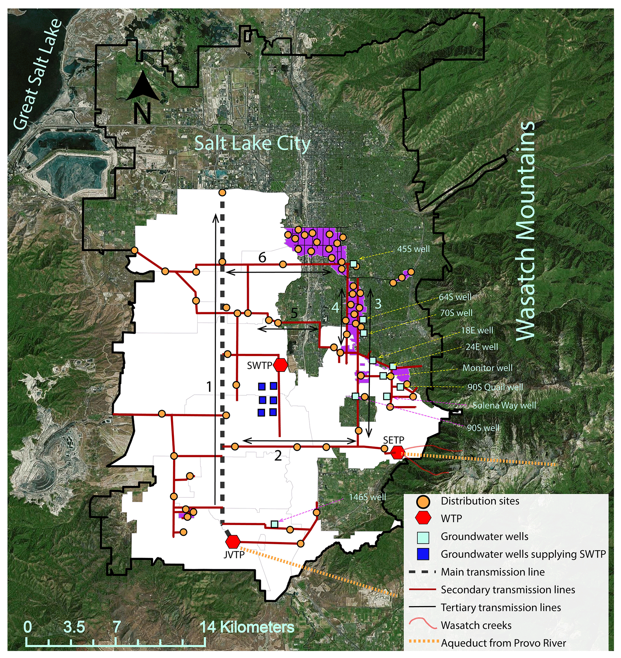
Figure 1Jordan Valley Water Conservancy District (JVD) wholesale area (white) and Jordan Valley retail area (purple) within the Salt Lake metropolitan valley (black border). Water from wells shown in light blue color is pumped directly into the transmission lines on which they are located. The aqueducts from the Provo River and the Wasatch creeks are shown for illustrative purposes only. WTP: water treatment plant, JVTP: Jordan Valley Water Treatment Plant, SETP: Southeast Water Treatment Plant, SWTP: Southwest Water Treatment Plant. Source of base map: ESRI digital media.
In urban settings, stable isotopes and other geochemical tracers have been used successfully to understand effects of storm water control measures on urban streams (Jefferson et al., 2015), detect infiltration rates in urban sewers (De Bénédittis et al., 2005; Kracht et al., 2007), partition waste water and groundwater in urban sewers (De Bondt et al., 2018), and determine the age of drinking water in PWSS (Waples et al., 2015). Recent studies have also shown that stable isotopes of tap water in urban areas can be used to characterize active water management practices, identify linkages between socioeconomic factors and water management practices, and quantify the effects of climate variability on water resources (Ehleringer et al., 2016; Jameel et al., 2016; Tipple et al., 2017; Zhao et al., 2017, Wang et al., 2018).
Here, we collaborated with the Jordan Valley Water Conservancy District (JVD, also referred to as Jordan Valley District) to conduct an isotopic survey of waters from their service area within the Salt Lake Valley metropolitan area (SLV) of northern Utah, USA (Fig. 1). JVD is a multi-source public water distribution network (Fig. 1) and we attempt to understand mixing between water sources at various sites (subsequently referred to as distribution sites) distributed on the transmission lines using SIW. This work extends the earlier work of Jameel et al. (2016) and Tipple et al. (2017) beyond identifying broad water management patterns of a PWSS and explores the capacity of SIW to provide quantitative, spatially and temporally resolved estimates of source contributions within a well-defined and characterized PWSS.
We conducted our study during a 6-month period (May–October 2015), and using information on the production volume from the different sources, we analyze the stable isotope data at a monthly resolution within a Bayesian framework to generate quantitative estimates (with uncertainty) of the contribution of individual sources at the distribution sites. These analyses reveal basic information on supply and transport dynamics within the system, reflecting the physical structure of the supply system and the geographic distribution of sources. Finally, we combine the monthly analyses to characterize the spatial structure of the system in terms of contribution areas for the different sources across the supply network. Our results suggest that SIW-based Bayesian isotope mixing models (BIMM) could be a powerful and useful tool to interrogate PWSS, provide observational validation to hydrodynamic models, track contaminants and disinfectants within the supply system, and monitor water rights in PWSS managed by or for multiple stakeholders. This technique can be particularly useful in understanding water management practices of urban centers in the developing world that are undergoing rapid expansions and are generally decentralized, which makes conventional hydrodynamic techniques difficult to apply.
2.1 Site description
The Jordan Valley District is a wholesale supplier to 17 water districts in the Salt Lake Valley (USA) and retails directly to several locations in SLV located primarily on the northeastern part of the valley (known as the Jordan Valley retail area, Fig. 1). As a wholesaler, Jordan Valley District sells water to these 17 districts from fixed locations on their distribution line and is not responsible for managing and distributing water in these districts beyond the transfer point.
In general, JVD relies on 3–5 sources at any given time to supply water to its service area; however, during the summer season (June–August), an additional 5–7 sources are often used to meet increased municipal water demand (personal communication, JVD operations manager). Water is sourced primarily through the Provo River system (>75 % of total water supplied annually) and is supplemented with water from Wasatch creeks and groundwater wells depending on demand. The Wasatch creek sources carry runoff from snowmelt in the Wasatch Mountains (Fig. 1) and are used only in spring and early summer. There are approximately 25 active groundwater wells managed by the Jordan Valley District. Not all wells operate simultaneously, rather only two to five wells operate at any given time and the operating wells are rotated every few months due to contractual obligations and also to avoid overexploitation.
Jordan Valley District operates three water treatment plants (WTP). The Jordan Valley Water Treatment Plant (JVTP, also referred to as Jordan Valley Treatment Plant in the text) is the largest water treatment plant and is situated at the southern end of the valley (Fig. 1). It has a maximum operational capacity of 681 374 m3 per day (80 million gallons per day) and treats water from the Provo River. The Southeast Water Treatment Plant (SETP, also referred to as Southeast Treatment Plant in the text) is a significantly smaller WTP with a maximum operational capacity of 75 708 m3 per day (20 million gallons per day) situated on the southeastern side of the valley. It also treats water from the Provo River, but during spring and early summer (Mid-April to June) most of the water treated at SETP is from the Wasatch creeks. The Southwest Water Treatment Plant (SWTP) has a maximum operational capacity of 26 497 m3 per day (7 million gallons per day), is located in the middle of the valley, and treats water from groundwater wells located near the treatment plant. Groundwater wells supplying the SWTP (shown as dark blue squares in Fig. 1) have a high salt concentration and require extensive purification before being pumped into the distribution system. In contrast, groundwater wells located on the eastern side of the valley (shown as light blue squares in Fig. 1) have lower concentrations of dissolved salts and do not require additional treatment before entering the distribution system (personal communication, JVD operations manager).
The Jordan Valley District water distribution system consists of one primary (Fig. 1), several secondary (line 2 through 6, Fig. 1), and numerous tertiary transmission lines. Water can move in either direction in all the transmission lines; however, in transmission line 1, water primarily moves from south to north. Water from Jordan Valley Treatment Plant is pumped directly into transmission line 1 and water from Southeast Treatment Plant is pumped into transmission lines 2 and 3 (Fig. 1). Water from Southwest Treatment Plant is supplied mainly to residential areas in the vicinity of the WTP (these supply connections are not shown in Fig. 1), though some water from SWTP is also pumped directly into transmission lines 5 and 6 (bypassing line 1). Water from wells in the eastern side of the valley is pumped directly into the transmission lines on which the respective wells are located. Most of the secondary transmission lines are interconnected via tertiary and quaternary lines (not shown in Fig. 1 except for the tertiary connections in the Jordan Valley retail area).
2.2 Sample acquisition and processing
Each month, from May to October 2015, we sampled water at sources contributing to the Jordan Valley District service area and at numerous locations (distribution sites or simply sites, Fig. 1) on the Jordan Valley District transmission lines. Source water samples were collected as effluent from the WTPs and directly from the groundwater wells, while distribution site samples were collected from monitoring taps on the transmission lines. For source water samples obtained from water treatment plants, we measured the pre- and post-treatment (i.e., influent to the WTP and effluent from the WTP) isotopic composition of the water. We did not observe any significant isotopic difference between pre- and post-treatment samples (differences in δ2H and δ18O less than 0.7 ‰ and 0.2 ‰, respectively). Distribution sites and surface water sources (Provo River and Wasatch creeks) were sampled one to three times per month. Groundwater wells were sampled one to five times, respectively, during the entire study period (May to October 2015). When a given well was not sampled in its month of operation, the mean value observed for the same well during other month(s) of our study period was used to characterize water supplied from that well. This substitution was justified given that previous work showed little temporal variability in the isotope values of water supplied from Salt Lake Valley groundwater wells (Jameel et al., 2016). The distribution sites are routinely monitored by Jordan Valley District for water quality analysis and are located across the supply network based on Jordan Valley District's monitoring program. As such, the distribution sites are more densely distributed in the Jordan Valley retail area because Jordan Valley District is responsible for water quality monitoring within this area. In other districts, where Jordan Valley District wholesales water, samples were collected only from the primary and secondary transmission lines.
Southeast Treatment Plant water was sourced mostly from the Wasatch creeks in May and June 2015, and from the Provo River from July to October 2015. Jordan Valley Treatment Plant water was sourced from the Provo River for the entire period of analysis. Therefore, we considered SETP and JVTP as separate sources in May and June and as a single source from July to October. Isotope ratios for effluent from SETP and JVTP were not statistically different between July and October (Hotelling multivariate t test, p>0.05, n=9). Additionally, groundwater wells situated close to each other and having similar isotope values (differences in δ2H and δ18O less than 0.5 ‰ and 0.1 ‰, respectively) were also combined together for our analyses (such as wells 64S and 70S in June, July, and August 2015).
2.3 Isotope analysis
Samples were collected in 4 mL clean glass vials and stored in a refrigerator at 4 ∘C prior to analysis. The samples were analyzed within a few weeks of collection at the Stable Isotope Ratio Facility for Environmental Research (SIRFER) facility, University of Utah, on a cavity ring-down spectrometer (L2130-i; Picarro, Inc., Santa Clara, CA) following protocols described in Good et al. (2014), following van Geldern and Barth (2012). Values are reported in δ notation: ), where Rsample and Rstandard are the 2H ∕ 1H or 18O ∕ 16O ratios for the sample and standard, respectively, and the VSMOW standard is referenced (Coplen, 1988). Accuracy and precision were checked using a secondary laboratory reference water, and the analytical precision for these analyses was ±0.3 ‰ for δ2H and ±0.03 ‰ for δ18O (±1 SD).
2.4 Bayesian mixing model and statistical analyses
We estimated the fractional contribution of the different sources at the distribution sites for each month using a Bayesian isotope mixing model. The advantages of a Bayesian approach include (1) simultaneous analysis of both isotope ratios (δ2H and δ18O), (2) inclusion of prior information into the statistical analysis (such as those from previous studies, ancillary data, and subjective knowledge), (3) explicit incorporation of analytical and sampling uncertainties into the model, and (4) robust estimates of uncertainty and quantification of most likely solutions in an underdetermined system (number of sources greater than number of isotopes plus 1).
The Bayesian mixing model described here is similar to those used in other studies involving stable isotope data (Ogle and Barber, 2008; Parnell et al., 2010; Cable et al., 2011; Mailloux et al., 2014). For our analysis, we first define the likelihood of the source isotope data. For this, we assumed that the different isotopic observations of each source (J) for a given month are coming from a bivariate normal distribution with a mean vector [μδ2HJ, μδ18OJ] and a precision matrix (ΩJ) inverse of a covariance matrix) that reflects the temporal variability in the source isotope values. The bivariate normal distribution accounts for the potential correlation between δ2H and δ18O. By using a joint distribution, and its associated variance–covariance matrix, we capture both the individual variability and the co-variation. Thus,
where δ2H1J…δ2HNJ and δ18O1J…δ18ONJ are the N observations of δ2H and δ18O of source J for that month, [μδ2HJ, μδ18OJ] is the mean vector, and ΩJ is the precision matrix. Similar to the source model, we assumed that for a supply site (I), the monthly averaged isotope values [δ2HI, δ18OI] follow a bivariate normal distribution with mean vector [μδ2HI, μδ18OI] and a precision matrix (ΩI). Thus, for a supply site (I),
The mean stable isotope values of the supply site can also be expressed as a mixing model, where the mean value for supply site I (μδ2HI, μδ18OI) is the sum of the mean values of the sources weighted by their fractional contributions. Therefore, if K sources were used in a given month, (μδ2HI, μδ18OI) for each supply site (I) is denoted by
where fJ is the proportional contribution from a given source J at supply site I and is our parameter of interest, i.e., the parameter to be estimated by the BIMM. Values of f were described using the Dirichlet distribution, a multivariate generalization of the beta distribution that follows the mass-balance constraint, i.e., and . The Dirichlet distribution is characterized by parameter vector , such that the mean value associated with each f is .
In Bayesian analysis, the parameters to be estimated are initially assigned values (or distributions) that are believed to be the best estimate of the parameters. These initial values are referred to as prior values. After observing the data, the initial (or prior) values of the parameters are updated, and posterior values estimates of the parameter values are obtained. Please refer to Parnell et al. (2010) and Hoff (2009) for more detailed information on Bayesian isotope mixing model and Bayesian statistical methods, respectively. In our analysis, the parameters to be estimated were the fractional contribution of the different sources (f′s) at the distribution sites. We therefore assign prior values to f′s that were then updated using the observed isotope ratios data at the distribution sites (μδ2HI, δμ18OI) to obtain the posterior f′s.
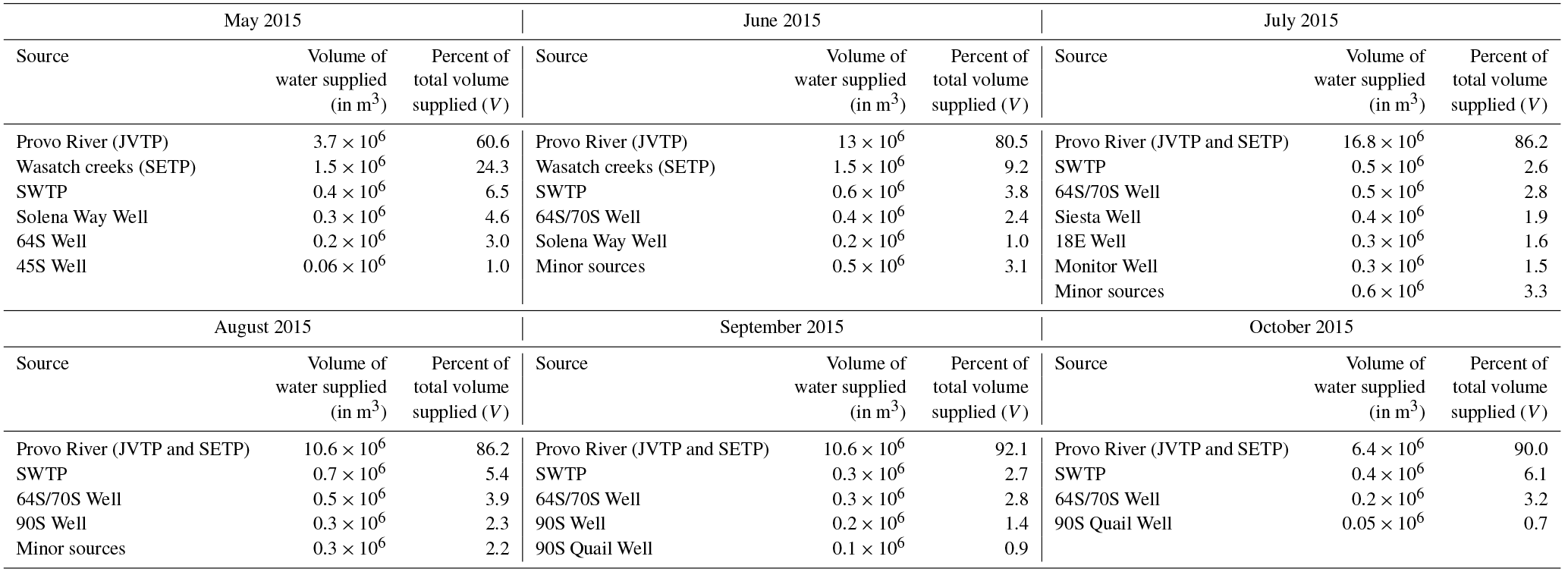
Table 1Volumetric contribution of each source and their proportional fractional contribution (V) for each month from May to October 2015. Monthly supply data were provided by Jordan Valley Water Conservancy District.Values were rounded to 1 decimal place except for 45S Well in May 2015 and 90S Quail Well in October 2015.
In general, if no information exists about the parameters, they are assigned a non-informative prior value. The default non-informative prior assigned to the Dirichlet distribution is the Jeffreys prior, where each element of the vector α is assigned a value of K−1 (with K being the number of sources) (Parnell et al., 2010). However, if preexisting information about the parameters exists, they are assigned informed prior values. In our case, we had existing information on the volumetric contribution of each source to the water system as a whole (obtained from JVD, Table 1) as well as the distance between the sources and the distribution sites, each of which, we assert, should affect the probability that a given source supplied water to a given site. Therefore, we assigned prior values for each supply site based on this information. First, we assumed that the probability of a source supplying a given distribution site was proportional to the volume of water that source supplies to the JVD distribution system (Table 1). Thus, sources contributing more water to the JVD system have a higher probability of supplying water to any given site than do lower-volume sources. Second, we assumed that the probability of a source supplying water to a given site was inversely proportional to the distance between the source (e.g., water treatment plant or well location) and the distribution site. Thus, sources closer to a distribution site have a higher probability of supplying water at that site. We combined both pieces of prior information to obtain a normalized prior estimate, as described below.
In the first step, we calculated prior weights for the Dirichlet parameters for each source (J) based upon the proportional volume of water produced (V) by that source:
Second, we distance weighted each source's prior inversely based upon its distance (D) from supply site I:
We then combined the volume and distance weighted priors to obtain a prior estimate of the mean contribution from source J at supply site I:

Figure 2Mean prior contribution of selected sources at the distribution sites for June 2015 based upon Eq. (6) described in Sect. 2.4. Distribution sites are shown as circles, and the color reflects the assigned prior contribution from the different sources. The source location is shown as a red diamond in each panel. The name of each source and its percent volumetric contribution (V) is shown above each panel.
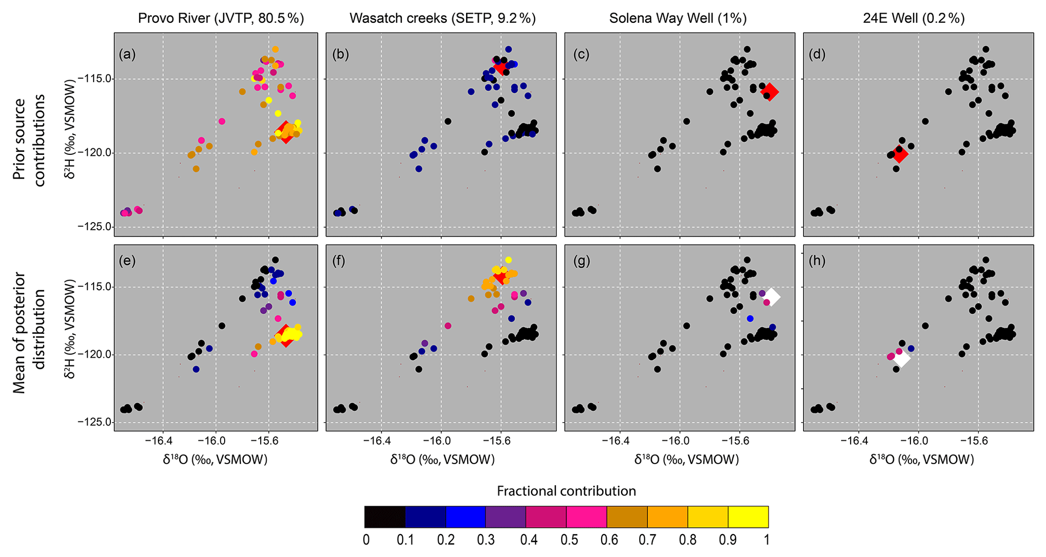
Figure 3Prior contribution of selected sources at the distribution sites (a–d) and mean posterior contribution of selected sources at distribution sites (e–h) in isotope space for June 2015. Red diamonds represent sources and the circles represent distribution sites. For clarity, diamonds in (a) through (h) have been enlarged and in (g) and (h) are shown in white. The name of each source and its percent volumetric contribution (V) is shown above each panel.
For example, if there were three sources supplying 3000, 1500, and 1500 m3 of water, respectively, to the JVD system that were located 4, 1, and 10 km away from supply site I, then the Dirichlet prior vector would be {0.3125, 0.625, 0.0625} for this site I.
Based upon the above-described method, the prior contributions of selected sources at the distribution sites for June 2015, in spatial and isotope space, are shown in Figs. 2 and 3, respectively. The prior values were then updated using the observed isotope values at the distribution sites (μδ2HI, δμ18OI) to obtain the posterior values of f′s. We estimated the posterior fractional (f) contributions to each site I from each source J using the JAGS software package (Plummer, 2003), which can be integrated in the R statistical language using different R packages (Plummer, 2013; Denwood, 2016). We ran three parallel Markov chain Monte Carlo (MCMC) simulations for 300 000 iterations per chain, which were thinned every 50 steps. The first 40 000 iterations were discarded as burn-ins, providing us with 5200 samples for calculating the posterior statistics. We checked the convergence using the coda package (Plummer et al., 2006) and Gelman diagnostics (Gelman et al., 2014). All statistical analysis was performed in R (R core team, 2018).
2.5 Model results interpretation and cross-validation
For qualitative interpretation and to identify spatiotemporal variations in the association between sources and distribution sites, we considered any distribution site that our mixing analysis suggested was receiving more than 70 % (mean contribution) of its water from a single source to be supplied predominantly by that source. Sites where the analysis suggested less than 70 % water came from a single source were considered to receive water from multiple sources.
For each month, we compared the fractional production volume of each source with the fraction of the service area that our analysis suggested was served by the source. We calculated the areal contribution of the different sources for each month as a cross-check of the results obtained by BIMM. As a first-order approximation, we expected strong agreement between volumetric and areal contribution of a source as the area supplied by a source should be proportional to its volumetric supply. To calculate the areal coverage of a given source, we first calculated the area of influence (AI) of each site on the transmission line, defined as the area of the Thiessen polygon associated with the site. For each source J, values of AI were multiplied by the mean fractional contribution from that source (fI, J). The resulting values were summed across all distribution sites and divided by the total area of Jordan Valley District supply region to obtain the areal coverage (A) of that source.
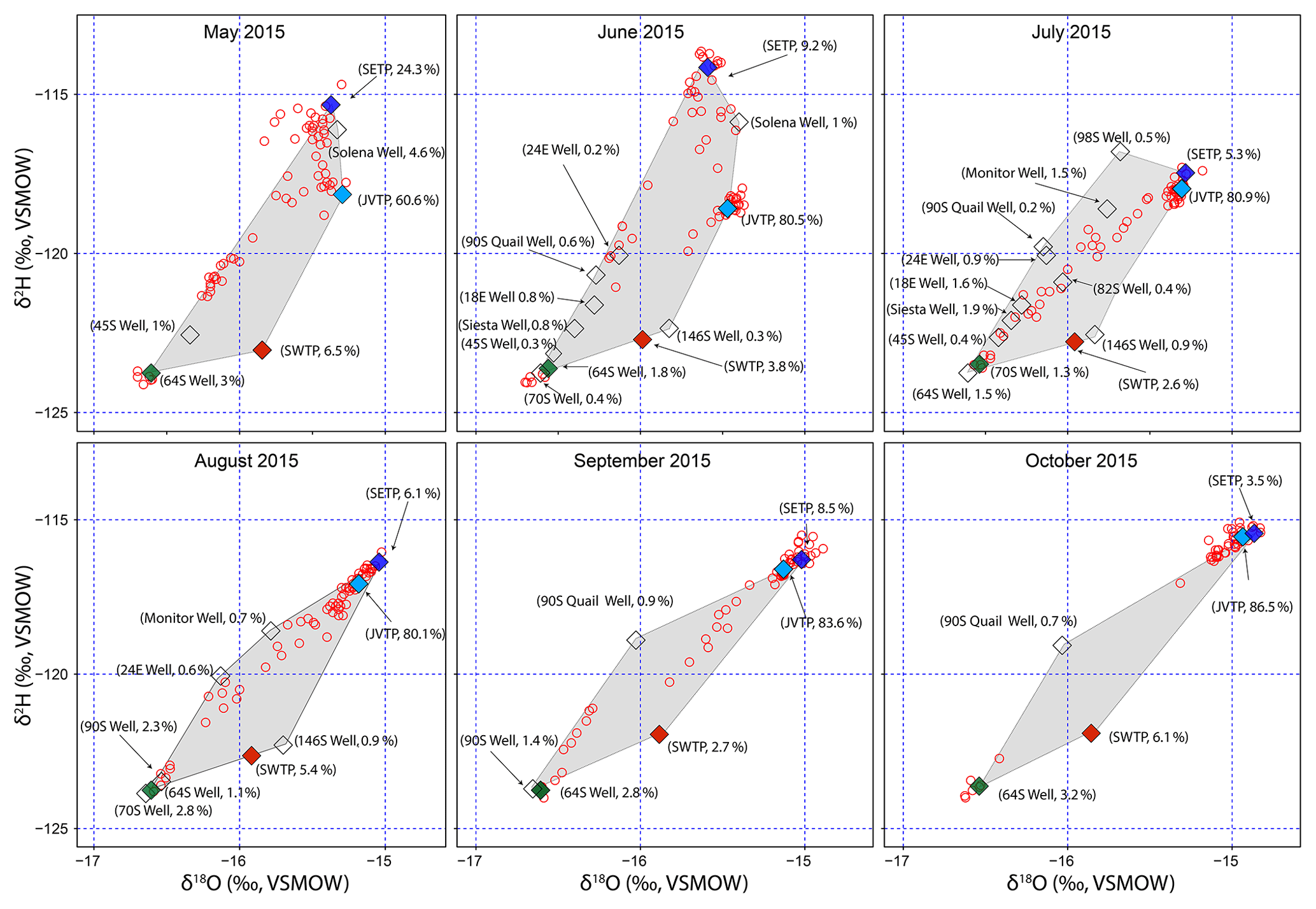
Figure 4Sources and distribution site isotope ratios from May to October 2015. Red hollow circles and diamonds represent distribution sites and sources, respectively. The four major sources (JVTP, SETP, SWTP, and 64S Well) have been colored light blue, dark blue, orange, and green, respectively. The grey region is the convex hull of the sources (defined as the minimum area enclosing all the source isotope values). The percentage value besides the name of the source represents the total volume of water supplied by the source in the given month.
3.1 Sources and distribution sites' isotope ratios
Source water isotope values, measured across all months, ranged from −16.6 ‰ to −14.9 ‰ for δ18O and −122.5 ‰ to −114.1 ‰ for δ2H. Four sources (JVTP, SETP, SWTP, and well 64S) operated for the entire sampling period, and other sources operated intermittently. For each month, approximately 90 % (or more) of the water was supplied by the three WTPs (JVTP, SETP and SWTP), with the majority being supplied by JVTP (Table 1). Groundwater wells situated on the eastern side of the valley contributed approximately 10 % of the total water supplied each month, with well 64S supplying 1–3 % of the total volume each month.
The isotope values of SWTP and well 64S were distinct from each other and from those of JVTP and SETP for all months (Fig. 4). Isotope ratios of JVTP and SETP water were distinct (Hotelling multivariate t test, p<0.05, n=6) for May and June 2015 only. From July 2015 onwards, water from the Provo River was used by both of these WTPs; therefore, similar isotope ratios were expected. Well 64S had the lowest isotope ratios measured for any source and exhibited the highest deuterium excess values (∼10 ‰) among all the wells, where deuterium excess is defined as δ2H–8δ18O (Dansgaard, 1964). Values from SWTP, in contrast, showed evidence for evaporative isotope effects, with high δ18O values and relatively low deuterium excess (∼4.2 ‰). JVTP isotope ratios increased from June to October 2015, as did SETP isotope ratios from July to October 2015, which can be due to evaporative enrichment of the heavy isotopes in upstream reservoirs of the Provo River system from spring to fall (mean d excess for JVTP decreased from 5.1 ‰ in June 2015 to 3.9 ‰ in October 2015; see Table S1 in the Supplement for monthly deuterium excess values).
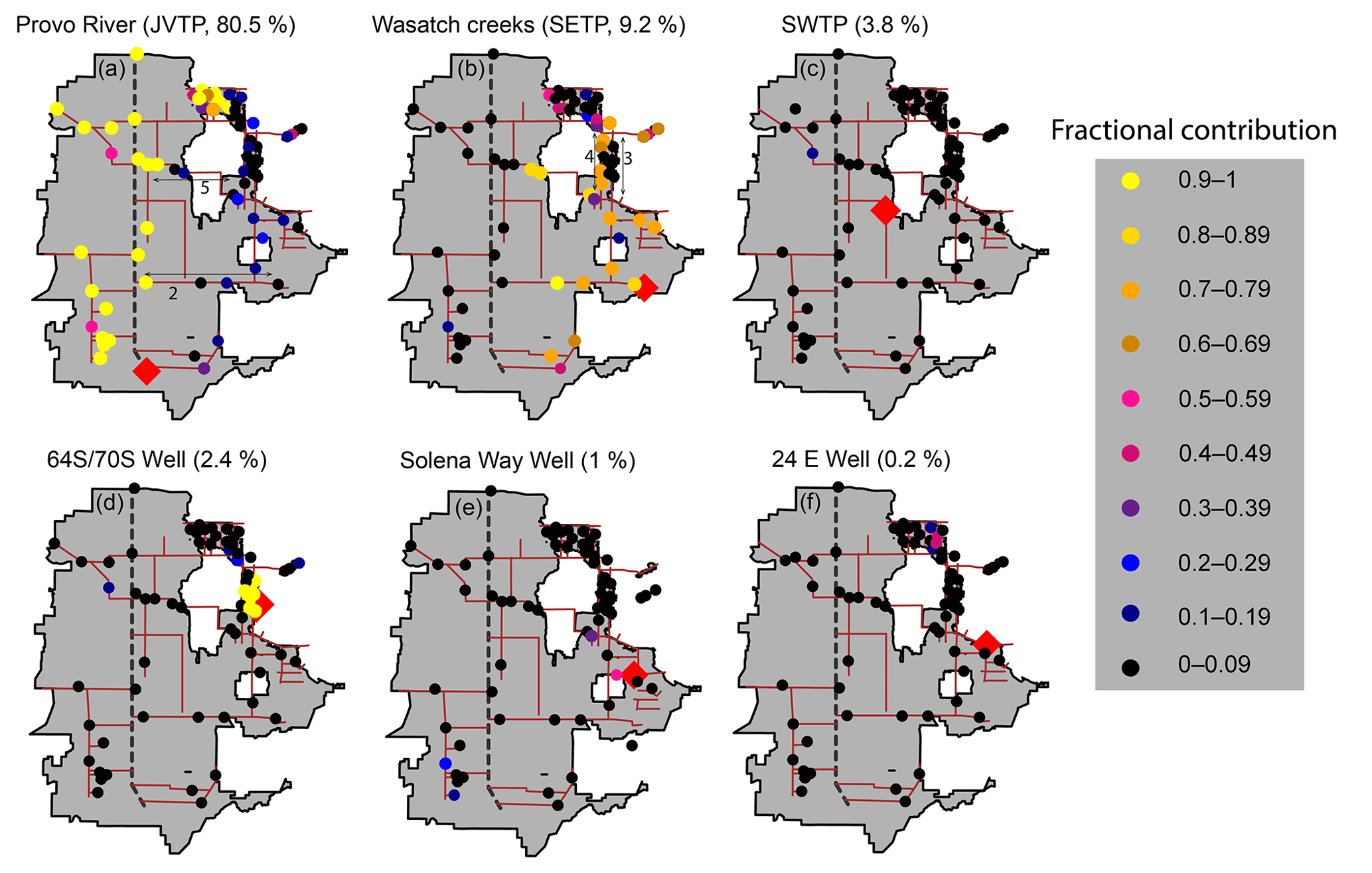
Figure 5Mean of the posterior contribution of selected sources at the distribution sites for June 2015. Distribution sites are shown as circles and the color reflects the mean of the posterior contribution from the respective source at that site. The source in each panel is shown as a red diamond. The name of the source and its percent volumetric contribution (V) is shown above each panel. Transmission lines 2 and 5 are shown in (a) and lines 3 and 4 are shown in (b).
The most and least negative isotope values of water from distribution sites were similar to the values observed for well 64S/70S and SETP, respectively. With the exception of a few sites in the May 2015 survey, distribution site isotope ratios fell within the convex hull defined by the source waters (Fig. 4). For each month, a number of distribution sites exhibited values similar to JVTP (Fig. 4). Clustering of supply site values was also observed near well 64S and SETP source values. At no point during the study did we observe any distribution sites with isotope values similar to those of SWTP source water (Fig. 4). For all months except October, approximately 20 %–30 % of the supply site values did not cluster near any major source, but rather were situated between sources. This pattern is consistent with expectations for mixing of water from multiple sources within this PWSS.
3.2 Source contributions at the distribution sites
We first illustrate the implementation of the BIMM for June 2015 (Fig. 5). Our model builds upon the work of Jameel et al. (2016) and Tipple et al. (2017), but goes beyond their analyses of identifying district level water management patterns by providing quantitative, spatially and temporally resolved estimates of source contributions at specific locations throughout the Jordan Valley supply system.
According to our model, the majority of the distribution sites (45 out of 65) received most (>70 %) of their water from a single source. At all of these sites, the dominant source identified was either JVTP (24 sites, Figs. 3e and 5a), SETP (15 sites, Figs. 3f and 5b), or well 64S/70S (6 sites, Fig. 5d). This shows that three of the four largest sources operating at the time dominated the supplies of a large number of sites and that the number of sites served by these sources was approximately proportional to the volumetric contribution from each source. Our analysis suggests that the remaining 20 sites did not receive water predominantly from a single source, but had contributions from multiple sources.
Most of the sites receiving large proportional contributions from JVTP, SETP, and well 64S/70S were located on the transmission lines known to be directly connected to these sources (Fig. 5a, b and d). In contrast, distribution sites distant from all sources were more likely to exhibit mixing between multiple sources. During June 2015, all but three sites in the Jordan Valley retail area showed evidence for source mixing.
Our model output, in context with known physical infrastructure (i.e., pipelines) and geographic locations of the sources, suggested patterns of source–supply connectivity within the JVD. Our results suggest (1) subtle differences in mixing proportions among distribution sites receiving water mainly from the two largest sources (JVTP and SETP), (2) limited mixing at distribution sites located on transmission lines receiving water from multiple sources, and (3) bypassing of a specific transmission line during water transport. Below, we discuss each of these observations in more detail.
For sites on the western portion of the Jordan Valley District, the model-inferred mean JVTP contributions were uniformly large (>90 %), suggesting that JVTP was likely the dominant source supplying water to these sites (Fig. 5a). This was expected, as most of these sites have limited connectivity to other sources apart from the SWTP. In contrast, our model suggested that most distribution sites receiving water predominantly from the SETP had mean contributions of SETP waters of 70 %–90 % (Fig. 5b). This likely reflects minor contributions of water from JVTP and several smaller sources in close proximity to SETP (Fig. 5a, e and f), implying that, although these sites are served chiefly by a single source, they also receive a significant fraction of water from other sources and thus are exposed to any supply or contamination issues associated with those minor sources. According to our model, sites receiving more than 60 % of water from SETP had an average contribution of 12 % from the minor sources with some sites receiving as much as 27 % of water from the minor sources.
Our model suggested limited mixing between JVTP, SETP, and other minor sources for distribution sites located on transmission lines 2 and 5 (Fig. 5a) that could receive water from all of these sources. Distribution sites on these lines mainly received water either from JVTP or SETP (more than 70 %), with contributions from other sources generally less than 30 % (Fig. 5a and b). Considering that JVTP supplied more than 80 % of all water in June 2015, we expected mixing and a large contribution from the JVTP at sites along these transmission lines (lines 2 and 5). One factor that may have caused limited mixing between these sources within the supply lines is the higher elevation of SETP (1532 m) and other minor sources on the eastern side of the valley compared to JVTP (1424 m). We suggest that the higher gravitational potential energy of water introduced from SETP and minor sources may create a pressure differential that limits mixing between these two sources; however this remains a hypothesis to be tested.
Our model suggested negligible presence of SETP water in transmission line 3 (<15 %), whereas the mean contribution of SETP in a closely running parallel transmission line 4 was high (>60 %, Fig. 5b). This result implies that water moving northward from SETP bypassed line 3. This is most likely due to the presence of well 64S/70S (Fig. 5d) on line 3, which our results suggested was the principal source to all the sites on line 3. This highlights the ability of the isotope mixing model to capture small-scale interactions between sources and supply connections.
The BIMM presented here is blind to the actual physical connections in the Jordan Valley District service area. Nonetheless, our results closely match the specific linkages between sources and distribution sites along known transmission lines. The ability of BIMM to identify patterns of source–supply connectivity within this system suggests the potential to use similar isotope-based methods to obtain information from less documented public water supply systems.
3.3 Assessment of uncertainties and model limitations
In addition to providing point estimates of source water contributions, the BIMM also provides estimates of uncertainty. To analyze the uncertainties, we divided the isotope values of the distribution sites measured in June 2015 into three groups. Group 1 consisted of sites with isotope values similar to one of the major sources (Fig. 6a), group 2 consisted of sites with isotope values in-between the SETP and JVTP endmembers (Fig. 6b), and group 3 consisted of distribution sites with isotope values similar to one of the minor sources but significantly different from any of the major sources (Fig. 6c).
According to our model, all sites in group 1 had large contributions (>70 %) from one of the major sources (JVTP, SETP or 64S/70S wells), and we observed narrow 95 % credible intervals (CIs, ranging mostly from 0.6 to 1) for the proportional contributions from these sources (Fig. 7a and b). At these sites the CIs for other sources were also narrow and ranged from 0.0 to 0.3 (Fig. 7c–h), indicating high levels of confidence that other sources were minor contributors to these sites. The effectiveness of BIMM in providing tight and robust posterior distributions for group 1 sites is due to the strong similarity between source and distribution site isotope values in this group and the distinct isotope ratios of water from these sources relative to all others.
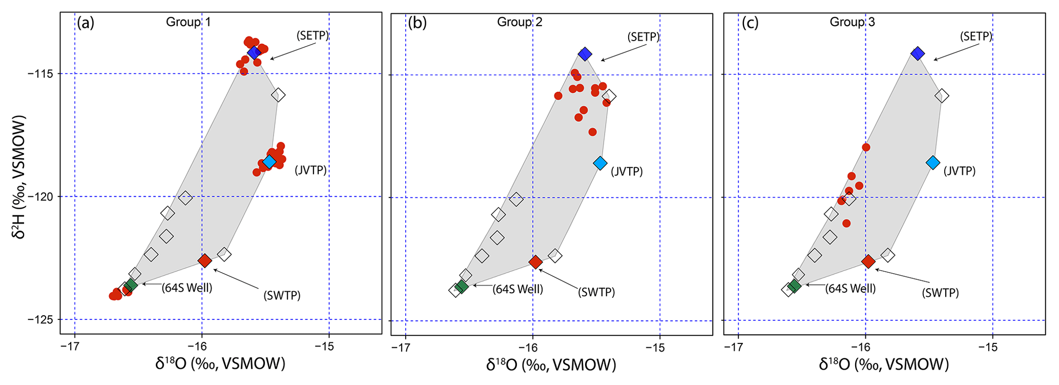
Figure 6Distribution sites and sources for June 2015 shown as red circles and diamonds. The four major sources (JVTP, SETP, SWTP, and 64S Well) have been colored light blue, dark blue, orange, and green, respectively, and are labeled. Minor sources are shown as hollow diamonds. (a) group 1, (b) group 2, and (c) group 3 distribution sites.
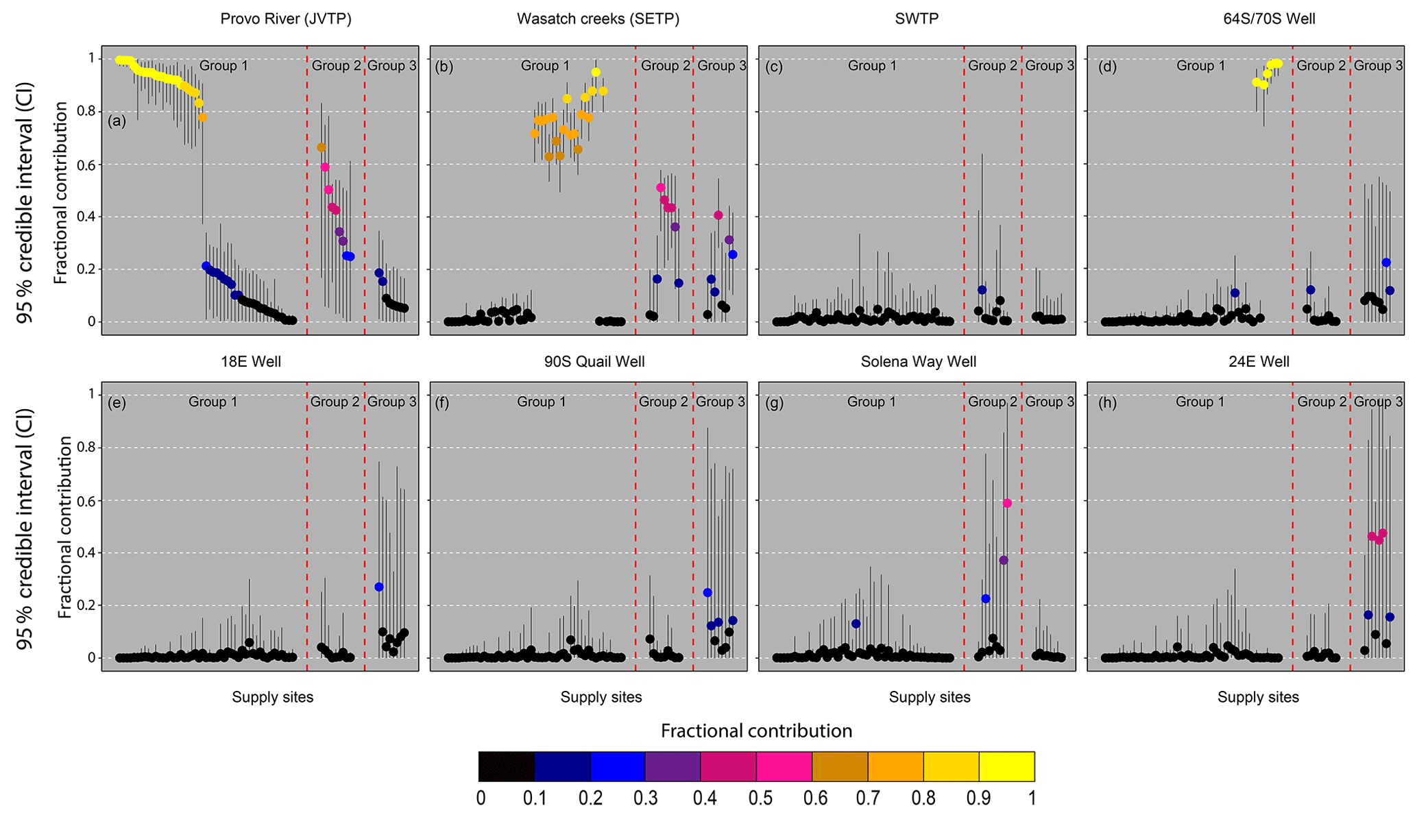
Figure 7Mean (circle) and 95 % credible interval (vertical black lines) associated with the source contributions at the distribution sites for the different groups for June 2015. Sites in (a) have been sorted with decreasing contribution from JVTP for each group. The same sorting order is maintained for (b–h).
For group 2 sites, the model predicted mixing primarily between water from the JVTP and the SETP (Fig. 7a and b), with contributions of 40 % to 60 % from each of these sources. According to our model, the contribution from the Solena Way Well was minimal at all group 2 sites except for a single site situated very close to the well (Fig. 5e). Given that the Solena Way Well contributed only 1 % of the total water to the system, dominance of JVTP and SETP water at most group 2 sites is reasonable. Further, most of the group 2 sites were situated in the Jordan Valley retail area, far from the Solena Way Well (>5 km, Fig. 5a, b and e). The CIs associated with different sources at these sites were larger than group 1 sites. Most of these sites had CIs ranging from 0.0 to 0.6 for JVTP (Fig. 7a), from 0.3 to 0.6 for SETP (Fig. 7b), and from 0.0 to 0.6 for the Solena Way Well (Fig. 7g). The tighter CIs of contributions from SETP compared to JVTP and Solena Way Well at these sites suggests that our model is more confident about the contribution from SETP (i.e., between 30 % and 60 %) compared to contributions from JVTP and Solena Way Well. As observed for group 1, the CIs associated with other sources were small, in general, ranging from 0.0 to 0.2. The advantages of including distance and volume effects in our model were reflected in this group, as our model preferred mixing between water from the JVTP and the SETP over possible mixtures between water from the Solena Way Well and other minor sources.
Group 3 exhibited isotope values that were distinct from all major sources and were similar to one or more minor sources. According to the model, no source (major and minor included) contributed more than 50 % (mean) at these sites. In general, for a given supply site in this group, our model assigned the highest mean contribution to the minor source with isotope ratios most similar to those of the supply site water (for example see Fig. 5e). The CIs associated with proportional contributions from the different sources were large, however, and for some sources ranged from 0.0 to 0.9 (Fig. 7h). This suggests that more than one possible source or multi-source mixture was consistent with the isotopic and prior constraints for these sites, resulting in identifiability issues that are commonly observed in isotope mixing models (Cable et al., 2011; Erhardt and Bedrick, 2013; Parnell et al., 2013). In our case, non-unique assignments for group 3 sites arose due to the presence of multiple sources with comparable isotope values near the distribution sites and also due to several probable potential mixing solutions between SETP, the 64S/70S Well, and these minor wells. The issue was compounded further by similar and low prior probabilities associated with the minor sources, making it difficult for the model to identify one distinct source as a major contributor.
Our results highlight the robustness as well as the limitations of our model. Both the use of informative priors and the comprehensive assessment and interpretation of uncertainty are likely to improve the quality of inferences drawn from our method. A key outcome of the priors specified here is that volumetrically minor sources were not identified as a major contributor to distribution sites, even though in many cases they had similar isotope values, except in cases where proximity provided additional evidence suggesting that they were likely sources. This result was also observed in July and August 2015. Consideration of credible intervals estimated in the analysis shows substantial and interpretable variation in the confidence of source water estimates among different sites. Even in cases where relatively high mean source contributions were assigned to a given site, robustness in the model solutions can be recognized through review of credible intervals and used to more accurately interpret these results.
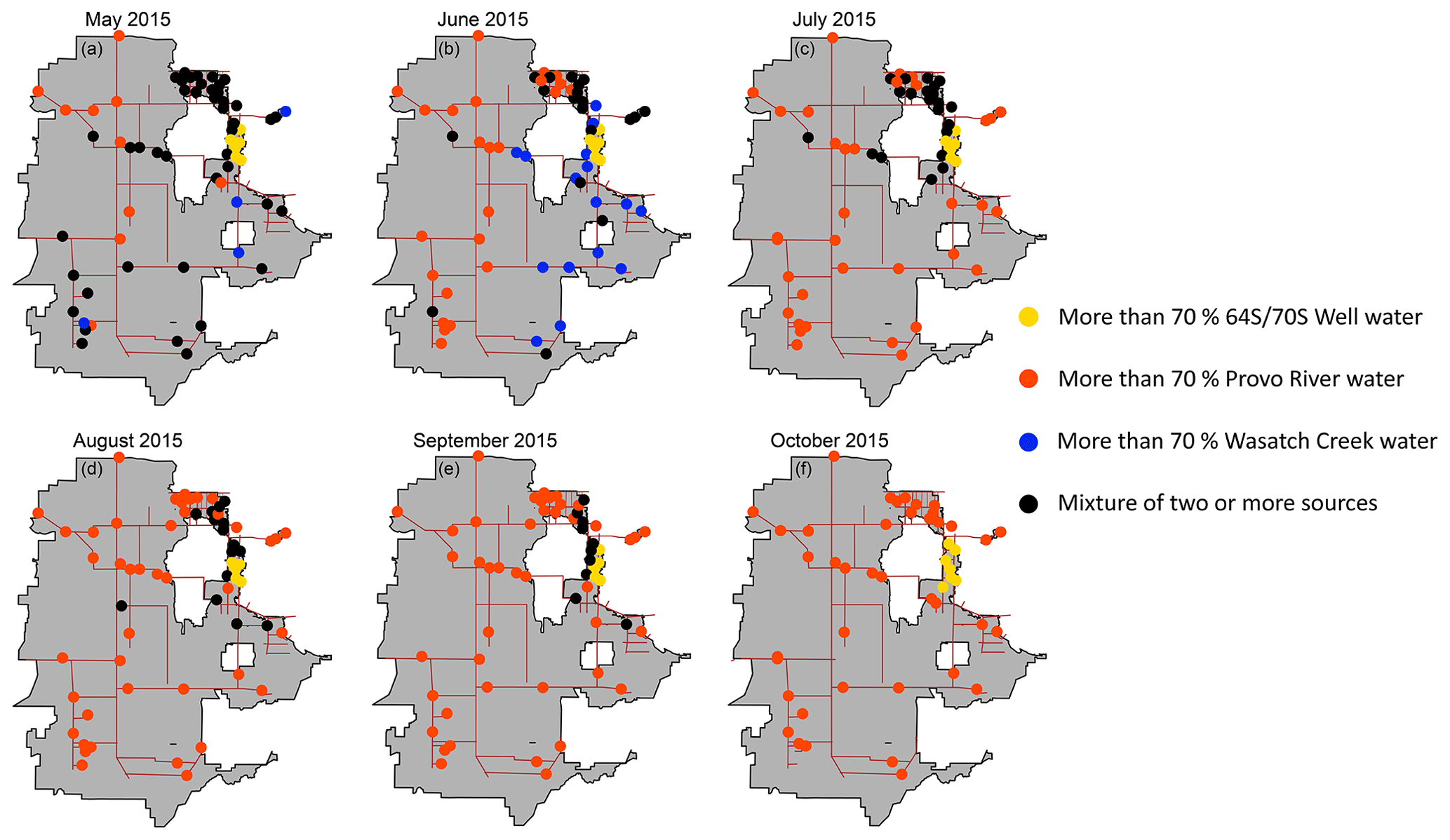
Figure 8Spatiotemporal variation in sources and distribution sites connectivity from May to October 2015. Distribution sites receiving more than 70 % water from a single source are shown in orange, blue, and yellow circles, and sites receiving water from multiple sources (less than 70 % water from a single source) are shown in black circle.
3.4 Spatiotemporal variations in source contributions
We extended our analysis to all months from May to October 2015, to assess changes in the patterns of water distribution as water demand, source types, and production volumes changed through the sampling period (Table 1).
Mixing between sources was high in May, with only 25 % of the distribution sites receiving more than 70 % of their water from a single source (Fig. 8a). For May, most of the distribution site values were intermediate to the source water values (Fig. 4), clearly indicating substantial mixing across most parts of the distribution system. A handful of supply site samples in May also fell outside of the convex hull defined by the sources, suggesting that our sampling may not have captured all contributing sources, but the conclusion of pervasive mixing is not likely to be affected by this omission. In contrast, our model suggests that almost 70 % of the sites were supplied chiefly by a single source in June and July, with this value increasing to more than 75 % in August and September (Fig. 8b–e). By October, the supply system had transitioned to a single, major source, and our results showed no significant mixing between sources for that month (Fig. 8f). Except for May 2015, where we observed large-scale mixing between different sources throughout the Jordan Valley District, distribution sites receiving water from multiple sources were limited mostly to the Jordan Valley retail area. Since this area is distant from all major sources and is surrounded by multiple transmission lines, mixing observed at the distribution sites is not surprising.
Perhaps the most surprising part of our analysis was our inability to detect contributions from SWTP at the distribution sites, even though this source supplied 3 %–5 % of total water production each month. Small contributions (10 % to 20 %) from this source were indicated at a couple of sites on transmission line 5, situated relatively far from SWTP, during June, July, and August 2015 (see Fig. 5c for June 2015). However, this source was not identified as the predominant source (i.e., >70 %) at any distribution site, including those closest to SWTP, during the study. According to the Jordan Valley District operations managers (personal communication) most of the water from SWTP is supplied to a residential area in the immediate vicinity of the treatment plant, and none of our distribution sites were located in this area. A small fraction of the SWTP water is routed to the western part of the Jordan Valley District, which is possibly reflected in our results suggesting minor contributions from this source to distribution sites along distribution line 5.
We combined our model output for different months to highlight variability and quantify the mean contribution for each source at the different distribution sites from May to October 2015 (Fig. 9). Our result suggests that most of the sites received water from multiple sources or switched sources during our analysis period, with the exception of a few sites receiving Provo River and 64S/70S Well water for all the 6 months. Our results show significant changes throughout the sampling period, highlighting the complex and dynamic operation of the distribution system. We have developed the monthly (Fig. 8) and 6-month averaged (Fig. 9) contribution from the different sources at the distribution sites based upon one to three samples collected each month; however, such maps can be developed at varying spatiotemporal scales depending upon the purpose and application of the method.
Figure 9Mean contribution of different sources at the distribution sites during May to October 2015. Sites in orange and yellow circles received water primarily (>70 %) from the Provo River and 64S/70S Well, respectively, throughout the entire sampling period. Sites in black circles received water from multiple sources or switched sources at least once during the sampling period.
Table 2Comparison between volumetric (V) and areal (A) contributions of the different sources from May to October 2015. V for each source was calculated from the monthly supply data of each source (see Table 1). A was calculated using methods described in Sect. 2.5. JVTP and SETP are considered as separate sources in May and June 2015 and combined sources from July to October 2015. Sources contributing less than 1 % of the total volume have been grouped together as “minor sources” for June, July, and August 2015. All values are in percent.
3.5 Model cross-validation
To validate the results obtained by BIMM we compared the volumetric contribution of the sources obtained from the Jordan Valley District (Table 1), with their areal contribution estimated using the BIMM. Volumetric and areal contributions were strongly and systematically correlated across all sources (Table 2). However, our model predicted that the Wasatch creeks supplied a larger fraction of the area than suggested by their volumetric contribution and that the Provo River sources supplied a smaller area than implied by volumetric production numbers in May and June (Table 2). This discrepancy could reflect differences in water demand across the service area, although most of the area our analysis suggests was served by the Wasatch creeks source is heavily populated, and the corridor served by the Provo River water source includes more industrial development that may over-consume water per unit area. Nonetheless, the overall similarity between the areal coverage estimated here and reported volumetric production numbers provides an additional line of evidence supporting the robustness of the BIMM.
3.6 Model improvements and future application of BIMM in other urban water systems
We have shown here that BIMM provides robust estimates of the contribution from different sources to distribution sites within a PWSS. In our analysis, the isotopic compositions of major sources were distinct, allowing our model to quantify the contribution from the major sources at the distribution sites with robust estimates of uncertainty across the supply system. However, for distribution sites with isotope values intermediate to candidate sources (group 3, Fig. 6), the specificity of our result was limited by non-unique solutions. These challenges and limitations could be addressed with the inclusion of other conservative tracers such as chloride, calcium, and strontium (and its stable isotopes) that might vary significantly between the different sources, thus providing additional constraints and improved model predictions. Additional system data, such as pressure, elevation gradients, and flow velocity within the system, might also be included within the model to improve accuracy.
A key prerequisite for future successful implementation of the BIMM in other PWSSs is that all sources in the PWSS be characterized and have significantly distinct isotopic and/or geochemical signatures. In PWSSs with negligible isotopic and geochemical variability between the sources, the capacity of the BIMM to characterize the system would likely be limited, and it will provide results with limited practical applicability. Finally, the BIMM approach is sample based and an appropriate sampling design would be required to accurately connect sources and distribution sites and extract meaningful information from the analysis. The sampling design should consider factors such as source compositions, system operations, water residence time, water demand, and population density within the PWSS to develop a robust sampling strategy for implementing the BIMM. It is essential to capture temporal variations, especially for surface water sources or other sources with rapid water transit time, to establish accurate association between the sources and distribution sites. In our analysis, our monthly sampling protocol captured the successive isotope enrichment of the Provo River source that was vital to the success of our model.
The framework applied here can be useful in establishing source water footprints, pathways, and interactions of water sources within PWSS. In cities across the developed world that use hydrodynamic models (such as EPANET and WaterCAD) (Rossman, 2002) to predict water quality and contaminant concentration across their supply systems, the accuracy of these predictions can be evaluated by comparing the observed and predicted stable isotopes in water (or other conservative geochemical tracers) at several distribution sites using the hydrodynamic model. In many developing and rapidly growing cities across the world where applying hydrodynamic models is challenging and difficult a framework similar to that shown here can be used to develop GIS products such as (1) service maps of the different sources, (2) regions within the PWSS undergoing seasonal source switching, and (3) regions serviced by surface or groundwater, respectively. These products can be helpful in moderating water rights issues, tracking of source- and WTP-related contaminants, evaluating the susceptibility to climatic variations, and investigating long- and short-term effects of source water quality on public health. Considering that stable isotope analysis of most water samples is now rapid (minutes) and inexpensive, geochemically based BIMMs offer an attractive tool for studying and monitoring PWSS in support of management and water security.
Water isotopes have been used extensively to monitor and understand the natural component of the water cycle (Gat, 1996; Aggarwal et al., 2005; Bowen and Good, 2015); however their application in urban water systems has been limited. Recent work has shown the capacity of water isotopes to record information about water management and quantify effects of climatic variability on water resources (Jameel et al., 2016; Tipple et al., 2017). Moving beyond the coarse resolution of these studies, our work has highlighted the ability of water isotopes to provide information about PWSS operation at a much finer scale. Here, we have shown the ability of water isotopes to provide estimates of the contributions of multiple water sources across a large metropolitan PWSS and inform our understanding of the physical structure and operation of the system. The method developed here does not rely on independent information about pipe networks, flow velocities, pressure gradients, or other details of the PWSS that are integral to hydrodynamic models, and thus it can be used to interrogate PWSS where this information is lacking or to independently validate hydrodynamic model results. Our application used only two isotope (δ2H and δ18O) measurements, supplemented with information on source volumes and geographic locations. Future applications could improve upon our work by including additional geochemical tracers and flow rates, adding additional information on distribution system structure (where available), collecting samples with higher spatiotemporal resolution, and refining the statistical model.
Raw data sets analyzed within this study can be accessed through the Waterisotopes database (http://waterisotopes.org, project ID 00065, Waterisotopes Database, 2018) and are available on Hydroshare (https://www.hydroshare.org/, Hydroshare, 2018). An R code to execute equations described in Sect. 2.4 for the month of June 2015 is provided in the Supplement, as are the source and distribution site data set for June 2015.
The supplement related to this article is available online at: https://doi.org/10.5194/hess-22-6109-2018-supplement.
YJ and GJB designed the project. YJ, SB, RPF and GJB developed the model. All authors contributed to interpreting the model results. YJ wrote the first draft of the paper. All authors contributed substantially to revisions and gave final approval for publication.
The authors declare that they have no conflict of interest.
We thank JVD for collaborating on this project and Heidi Nilsson for
collecting the water samples. This work was supported by U.S. National
Science Foundation grant 1208732.
Edited by:
Laurent Pfister
Reviewed by: Robert van Geldern and one
anonymous referee
Aggarwal, P. K., Froehlich, K. F., and Gat, J. R.: Isotopes in the water cycle, Springer, the Netherlands, 2005.
Bolar, A., Tesfamariam, S., and Sadiq, R.: Condition assessment for bridges: a hierarchical evidential reasoning (HER) framework, Struct. Infrastruct. Eng., 9, 648–666, 2013.
Boryczko, K. and Tchórzewska-Cieślak, B.: Analysis of risk of failure in water main pipe network and of delivering poor quality water, Environ. Prot. Eng., 40, 77–92, 2014.
Bowen, G. J. and Good, S. P.: Incorporating water isoscapes in hydrological and water resource investigations, WIREs Water, 2, 107–119, 2015.
Cable, J., Ogle, K., and Williams, D.: Contribution of glacier meltwater to streamflow in the Wind River Range, Wyoming, inferred via a Bayesian mixing model applied to isotopic measurements, Hydrol. Process., 25, 2228–2236, 2011.
Coplen, T. B.: Normalization of oxygen and hydrogen isotope data, Chem. Geol., 72, 293–297, 1988.
Dansgaard, W.: Stable isotopes in precipitation, Tellus A, 16, 436–468, https://doi.org/10.3402/tellusa.v16i4.8993, 1964.
Dawson, T. E. and Ehleringer, J. R.: Streamside trees that do not use stream water, Nature, 350, 335–337, 1991.
De Bénédittis, J. and Bertrand-Krajewski, J. L.: Measurement of infiltration rates in urban sewer systems by use of oxygen isotopes, Water Sci. Technol., 52, 229–237, 2005.
De Bondt, K., Seveno, F., Petrucci, G., Rodriguez, F., Joannis, C., and Claeys, P.: Potential and limits of stable isotopes (δ18O and δD) to detect parasitic water in sewers of oceanic climate cities, J. Hydrol., 18, 119–142, 2018.
Denwood, M. J.: Runjags: An R package providing interface utilities, model templates, parallel computing methods and additional distributions for MCMC models in JAGS, J. Stat. Soft., 71, 1–25, 2016.
Ehleringer, J. R., Barnette, J. E., Jameel, Y., Tipple, B. J., and Bowen, G. J.: Urban water – A new frontier in isotope hydrology, Iso. Env. Health Stud., 52, 477–486, 2016.
Erhardt, E. B. and Bedrick, E. J.: A Bayesian framework for stable isotope mixing models, Environ. Ecol. Stat., 20, 1–21, 2013.
Gabor, R. S., Hall, S. J., Eiriksson, D. P., Jameel, Y., Millington, M., Stout, T., Barnes, M. B., Gelderloos, A., Tennant, H., Bowen, G. J., Neilson, B. T., and Brooks, P. D.: Persistent Urban Influence on Surface Water Quality via Impacted Groundwater, Environ. Sci. Technol., 51, 9477–9487, 2017.
Gat, J.: Stable isotopes of fresh and saline lakes, in: Physics and chemistry of lakes, Springer, Heidelberg, 139–165, 1995.
Gat, J.: Oxygen and hydrogen isotopes in the hydrologic cycle, Annu. Rev. Earth Planet. Sci., 24, 225–262, 1996.
Gelman, A., Carlin, J. B., Stern, H. S., Dunson, D. B., Vehtari, A., and Rubin, D. B.: Bayesian data analysis, CRC press, Boca Raton, 2014.
Good, S. P., Mallia, D. V., Lin, J. C., and Bowen, G. J.: Stable isotope analysis of precipitation samples obtained via crowdsourcing reveals the spatiotemporal evolution of superstorm sandy, PloS One, 9, e91117, https://doi.org/10.1371/journal.pone.0091117, 2014.
Hanna-Attisha, M., LaChance, J., Sadler, R. C., and Schnepp, A.: Elevated blood lead levels in children associated with the Flint drinking water crisis: a spatial analysis of risk and public health response, Amer. J. Pub. Health, 106, 283–290, 2016.
Hoff, P. D.: A first course in Bayesian statistical methods, Springer, New York, 2009.
Hydroshare: https://www.hydroshare.org/, Search: First Author: Yusuf Jameel, last access: 20 April 2018.
Ismail, M. A., Sadiq, R., Soleymani, H. R., and Tesfamariam, S.: Developing a road performance index using a Bayesian belief network model, J. Frankl. I., 348, 2539–2555, 2011.
Jameel, Y., Brewer, S., Good, S. P., Tipple, B. J., Ehleringer, J. R., and Bowen, G. J.: Tap water isotope ratios reflect urban water system structure and dynamics across a semiarid metropolitan area, Water Resour. Res., 52, 5891–5910, 2016.
Jameel, Y., Stein, S., Grimm, E., Roswell, C., Wilson, A. E., Troy, C., Höök, T. O., and Bowen, G. J.: Physicochemical characteristics of a southern Lake Michigan river plume, J. Great Lakes Res., 4, 209–218, 2018.
Jefferson, A. J., Bell, C. D., Clinton, S. M., and McMillan, S. K.: Application of isotope hydrograph separation to understand contributions of stormwater control measures to urban headwater streams, Hydrol. Process., 29, 5290–5306, 2015.
Kabir, G., Tesfamariam, S., Francisque, A., and Sadiq, R.: Evaluating risk of water mains failure using a Bayesian belief network model, Euro. J. Oper. Res., 240, 220–234, 2015.
Kaushal, S. S.: Increased salinization decreases safe drinking water, Environ. Sci. Tech., 50, 2765–2766, 2016.
Kennedy, C. D., Bowen, G. J., and Ehleringer, J. R.: Temporal variation of oxygen isotope ratios (δ18O) in drinking water: implications for specifying location of origin with human scalp hair, Foren. Sci. Int., 208, 156–166, 2011.
Klaus, J. and McDonnell, J.: Hydrograph separation using stable isotopes: review and evaluation, J. Hydrol., 505, 47–64, 2013.
Kracht, O., Gresch, M., and Gujer, W.: A Stable Isotope Approach for the Quantification of Sewer Infiltration, Environ. Sci. Technol., 41, 5839–5845, 2007.
Larsen, T. A., Hoffmann, S., Lüthi, C., Truffer, B., and Maurer, M.: Emerging solutions to the water challenges of an urbanizing world, Science, 352, 928–933, 2016.
Liggett, J. A. and Chen, L. C.: Inverse transient analysis in pipe networks, J. Hydraul. Eng., 120, 934–955, 1994.
Mailloux, J. M., Ogle, K., and Frost, C. D.: Application of a Bayesian model to infer the contribution of coalbed natural gas produced water to the Powder River, Wyoming and Montana, Hydrol. Process., 28, 2361–2381, 2014.
Matheny, A. M., Fiorella, R. P., Bohrer, G., Poulsen, C. J., Morin, T. H., Wunderlich, A., Vogel, C. S., and Curtis, P. S.: Contrasting strategies of hydraulic control in two codominant temperate tree species, Ecohydrology, 10, https://doi.org/10.1002/eco.1815, 2017.
Najjaran, H., Sadiq, R., and Rajani, B.: Condition assessment of water mains using fuzzy evidential reasoning, paper presented at Systems, Man and Cybernetics, 2005 IEEE Intern. Conf., Waikoloa, Hi, USA, 3466–3471, https://doi.org/10.1109/ICSMC.2005.1571684, 2005.
Ogle, K. and Barber, J. J.: Bayesian data – model integration in plant physiological and ecosystem ecology, Progress in Botany, Springer, Heidelberg, https://doi.org/10.1007/978-3-540-72954-9_12, 281–311, 2008.
Parnell, A. C., Inger, R., Bearhop, S., and Jackson, A. L.: Source partitioning using stable isotopes: coping with too much variation, PloS One, 5, e9672, https://doi.org/10.1371/journal.pone.0009672, 2010.
Parnell, A. C., Phillips, D. L., Bearhop, S., Semmens, B. X., Ward, E. J., Moore, J. W., Jackson, A. L., Grey, J., Kelly, D. J., and Inger, R.: Bayesian stable isotope mixing models, Environmetrics, 24, 387–399, 2013.
Pietrucha-Urbanik, K.: Failure analysis and assessment on the exemplary water supply network, Eng. Fail. Anal., 57, 137–142, 2015.
Plummer, M.: JAGS: A program for analysis of Bayesian graphical models using Gibbs sampling, in Proceedings of the 3rd international workshop on distributed statistical computing, edited, p. 125, Vienna, Austria, 2003.
Plummer, M.: Rjags: Bayesian graphical models using MCMC, R package version, 3, 2013.
Plummer, M., Best, N., Cowles, K., and Vines, K.: CODA: convergence diagnosis and output analysis for MCMC, R news, 6, 7–11, 2006.
R Core Team.: R: A Language and Environment for Statistical Computing, R Found. for Stat. Comput., Vienna, Austria, 2018.
Rossman, L. A.: EPANET 2, User's Manual, Water supply and Water Resources Division, Nat. Risk Manag. Res. Lab., Cincinnati, USA, 2001.
Rozanski, K., Araguas-Araguas, L., and Gonfiantini, R.: Relation between long-term trends of oxygen-18 isotope composition of precipitation and climate, Science, 258, 981–985, 1992.
Schnoor, J. L.: Recognizing Drinking Water Pipes as Community Health Hazards, J. Chem. Educ., 93, 581–582, https://doi.org/10.1021/acs.jchemed.6b00218, 2016.
Tipple, B. J., Jameel, Y., Chau, T. H., Mancuso, C. J., Bowen, G. J., Dufour, A., Chesson, L. A., and Ehleringer, J. R.: Stable hydrogen and oxygen isotopes of tap water reveal structure of the San Francisco Bay Area's water system and adjustments during a major drought, Water Res., 119, 212–224, 2017.
van Geldern, R. and Barth, J. A.: Optimization of instrument setup and post-run corrections for oxygen and hydrogen stable isotope measurements of water by isotope ratio infrared spectroscopy (IRIS), Limnol. Oceanogr.-Meth., 10, 1024–1036, 2011.
von Grafenstein, U., Erlenkeuser, H., Brauer, A., Jouzel, J., and Johnsen, S. J.: A mid-European decadal isotope-climate record from 15 500 to 5000 years BP, Science, 284, 1654–1657, 1999.
Vörösmarty, C. J., McIntyre, P., Gessner, M. O., Dudgeon, D., Prusevich, A., Green, P., Glidden, S., Bunn, S. E., Sullivan, C. A., and Liermann, C. R.: Global threats to human water security and river biodiversity, Nature, 467, 555–561, 2010.
Waldrip, S. H., Niven, R. K., Abel, M., and Schlegel, M.: Maximum Entropy Analysis of Hydraulic Pipe Flow Networks, J. Hydraul. Eng., 142, 1–23, https://doi.org/10.1061/(ASCE)HY.1943-7900.0001126, 2016.
Waldrip, S. H., Niven, R. K., Abel, M., and Schlegel, M.: Reduced-Parameter Method for Maximum Entropy Analysis of Hydraulic Pipe Flow Networks, J. Hydraul. Eng., 144, 2333–2344, 04017060, 2018.
Wang, S., Zhang, M., Bowen, G. J., Liu, X., Du, M., Chen, F., Qiu, X., Wang, L., Che, Y., and Zhao, G.: Water source signatures in the spatial and seasonal isotope variation of Chinese tap waters, Water Resour. Res., 54, https://doi.org/10.1029/2018WR023091, 2018.
Waples, J. T., Bordewyk, J. K., Knesting, K. M., and Orlandini, K. A.: Using Naturally Occurring Radionuclides To Determine Drinking Water Age in a Community Water System, Envir. Sci. Tech., 49, 9850–9857, https://doi.org/10.1021/acs.est.5b03227, 2015.
Waterisotopes Database: http://waterisotopes.org, Query: Project ID: 00065, last access: 22 April 2018.
Yoo, D. G., Chung, G., Sadollah, A., and Kim, J. H.: Applications of network analysis and multi-objective genetic algorithm for selecting optimal water quality sensor locations in water distribution networks, KSCE J. Civ. Eng., 19, 2333–2344, 2015.
Zhao, S., Hu, H., Tian, F., Tie, Q., Wang, L., Liu, Y., and Shi, C.: Divergence of stable isotopes in tap water across China, Sci. Rep., 7, 43653, https://doi.org/10.1038/srep43653, 2017.