An assessment of trends and potential future changes in groundwater-baseflow drought based on catchment response times

Hellwig, Jost; Stahl, Kerstin

doi:https://doi.org/10.5194/hess-22-6209-2018

HESS | Articles | Volume 22, issue 12

Hydrol. Earth Syst. Sci., 22, 6209–6224, 2018
https://doi.org/10.5194/hess-22-6209-2018
© Author(s) 2018. This work is distributed under
the Creative Commons Attribution 4.0 License.

HESS | Articles | Volume 22, issue 12

Research article 03 Dec 2018

Research article | 03 Dec 2018

An assessment of trends and potential future changes in groundwater-baseflow drought based on catchment response times

Jost Hellwig and Kerstin Stahl Jost Hellwig and Kerstin Stahl Jost Hellwig and Kerstin Stahl

Faculty of Environment and Natural Resources, University of Freiburg, 79098 Freiburg, Germany

Correspondence: Jost Hellwig (jost.hellwig@hydrology.uni-freiburg.de)

Received: 04 May 2018 – Discussion started: 14 May 2018 – Revised: 02 Oct 2018 – Accepted: 31 Oct 2018 – Published: 03 Dec 2018

Abstract

Back to toptop

Drought is an important natural hazard with large impacts on society. Changes in drought characteristics have been studied for different parts of the hydrological cycle, but insights into changes of groundwater resources are obscured due to the lack of long-term observations and large heterogeneity of hydrogeological conditions. Moreover, predicted future changes in precipitation are uncertain and have a lagged effect on streamflow and groundwater. We investigated past changes and potential future changes in catchment baseflow as a reflection of groundwater drought for 338 headwater catchments across Germany based on catchments' characteristic response times. First, baseflow dynamics as a proxy of groundwater storage and outflow on a catchment scale were derived from streamflow records and related to precipitation input. Second, past trends in baseflow minima were calculated and attributed to climate and catchment controls. Last, response times and the timing of yearly baseflow minima were combined into estimates of the sensitivity to future precipitation changes. Baseflow response times of the studied headwaters are heterogenous across Germany, ranging from a few months to several years, and depend significantly on hydrogeological conditions. Few significant trends were found in past baseflow minima, and trends are highly dependent on the period of analysis. Based on the assumption of a typical regional scenario of increasing winter precipitation and decreasing summer precipitation, increases in hydrological drought hazard or no changes are projected for most parts of Germany. Catchments with longer response times can buffer interannual precipitation shifts, whereas catchments with fractured rocks are sensitive to summer precipitation decreases. These results urge for a surface water and groundwater management based on local groundwater response to precipitation and help to assess impacts of climate change on overall water supply.

How to cite

How to cite.

1 Introduction

Back to toptop

Drought is a natural phenomenon occurring in all compartments of the hydrological cycle. Accordingly, it is classified into meteorological drought, hydrological drought, agricultural drought, socio-economic drought and groundwater drought (Mishra and Singh, 2010). Due to the large number of people affected by drought and the high economic loss related to drought events (EC, 2007), it is important to enhance the understanding of drought processes considering projected changes in drought hazard, most importantly due to climate change. Empirical analysis of monitored hydrological time series remains an important tool with which to validate theory-based or model-derived hypotheses on these changes, since projected future changes are often uncertain. Particularly for the groundwater compartment there is a high diversity in response to climate input (Eltahir and Yeh, 1999; Green et al., 2011), making predictions even more difficult. Most of the empirical studies on long-term trends in drought hazard have focused on meteorological drought (e.g. Sheffield et al., 2012; Spinoni et al., 2017) and on hydrological drought (e.g. Stahl et al., 2010; Laaha et al., 2017). For groundwater drought, empirical trend analysis is difficult for two reasons: (i) groundwater time series are usually short or influenced by abstractions, and (ii) where long and natural time series are available, they only give point information.

Some countries and states now display groundwater level anomalies at observation wells as part of their drought monitoring (e.g. Switzerland: https://www.hydrodaten.admin.ch/de, last access: 28 November 2018; Bavaria: https://www.nid.bayern.de/grundwasser, last access: 28 November 2018). Studies on groundwater drought have mainly used borehole time series for index generation and statistical analysis (e.g. Bloomfield and Marchant, 2013; Bloomfield et al., 2015; Kumar et al., 2016; Van Loon et al., 2017; Heudorfer and Stahl, 2017; Leelaruban et al., 2017). The groundwater response to drought and its changes over time are typically very site specific, and observations are therefore hardly scalable from point to catchment scale (Kumar et al., 2016). However, larger regional-scale estimates of groundwater resources are relevant for effective groundwater management and adaptation to climate change. Model-based approaches for groundwater drought analysis and estimation (e.g. Peters et al., 2003, 2006; Tallaksen et al., 2009; Li and Rodell, 2015; Apurv et al., 2017) are one common way to get information on the catchment scale. There are also a few studies that analyse spring data (Fiorillo and Guadagno, 2012) or baseflow time series (Brutsaert, 2008, 2010; Fendeková and Fendek, 2012), two flux variables that provide a more integrative measure of the groundwater situation during drought.

To overcome the difficulties related to borehole data, in this study we use a baseflow approach to characterize groundwater drought on a catchment scale. We analyse a large dataset of long baseflow time series in central Europe. In this region groundwater is often used as drinking water, and aquifers act as an important buffer to climatic variability. Most droughts start with a deficit in precipitation, especially when precipitation falls as rain (Van Loon and Van Lanen, 2012). For the propagation from a meteorological to a groundwater drought different processes are relevant, i.e. attenuation, delay and pooling (e.g. Peters et al., 2003; Tallaksen et al., 2009; Heudorfer and Stahl, 2017). Therefore, the drought signal in groundwater storage not only depends on current meteorological conditions, but also the previous months are important. A catchment-specific timescale for this dependence may be called the catchment's response time. Response times have been analysed by correlations between groundwater depth and time series of precipitation accumulated for different periods. Studies have found that the response times for borehole water tables (Bloomfield et al., 2015; Van Loon et al., 2017; Leelaruban et al., 2017) or spring discharge (Fiorillo and Guadagno, 2012) vary strongly. Moreover, some studies suggest time lags for the highest correlations between precipitation and groundwater time series because of delayed groundwater response (Bloomfield et al., 2015; Fiorillo and Guadagno, 2012). However, when looking at monthly scales, this lag was always found to be quite small and often non-existent (e.g. Haas and Birk, 2017).

There are two approaches to identifying drought periods in a time series. The climatological approach is based on anomalies and often used also in hydrology to track the propagation of relative seasonal water deficits through the hydrological cycle (e.g. Barker et al., 2016; Kumar et al., 2016). The traditional hydrological approach is the “threshold level approach”, which defines streamflow droughts as events below a certain fixed limit and is therefore focused on actual low water availability (e.g. Yevjevich, 1967; Peters et al., 2006; Tallaksen et al., 2009). In this work we use the term drought according to the threshold level approach; thus we consider drought events as periods of low baseflow in absolute terms. If there is a distinct seasonal regime, droughts mostly occur in the dry season.

Recent work on central European low flows, i.e. periods when streamflow mostly consists of baseflow, found that climate change is expected to alter low flows (Marx et al., 2018; Forzieri et al., 2014; Van Vliet et al., 2015; Gosling et al., 2017). However, the sign and magnitude of change in central Europe are subject to model choice and emission scenario (Marx et al., 2018; Forzieri et al., 2014). Those modelling studies were focused on large river basins, and the change they predicted reflects strongly that of the precipitation change. Marx et al. (2018) found a high correlation between changes in annual precipitation sums and low flows. Stahl et al. (2012) found that hindcasting summer low flow trends with large-scale models suggests a too-homogenous spatial pattern of change compared to trends found in observations. Together with difficulties of models to capture the persistence of drought events in runoff generation found by Tallaksen and Stahl (2014), it can be assumed that some large-scale models do not necessarily resolve the heterogeneity of catchment storage and release for the hydrological response on a headwater catchment scale. However, recent drought events have demonstrated that especially headwaters are prone to groundwater-related drought impacts like shortages in water supply (Van Lanen et al., 2016). This coincides with findings that, independent from elevation, groundwater is an important catchment storage (Staudinger et al., 2017). Thus, predicting future changes in groundwater drought on a catchment scale will be a prerequisite for effective drought management.

Depending on the projected climate change, different scenarios of the future development of natural baseflow can be expected (Fig. 1). If there is an increase (decrease) in precipitation projected for the entire year, flow during the dry season is also expected to increase (decrease). However, if a seasonal shift of precipitation is expected, the future development of flow during the dry season is not that straightforward. It will depend on the timing of seasonal shift and dry period and on the catchment's characteristic response time to precipitation. Stölzle et al. (2014) found that for baseflow drought changes in precipitation are especially relevant during the recharge period, which is dependent on the hydrogeology of the catchment.

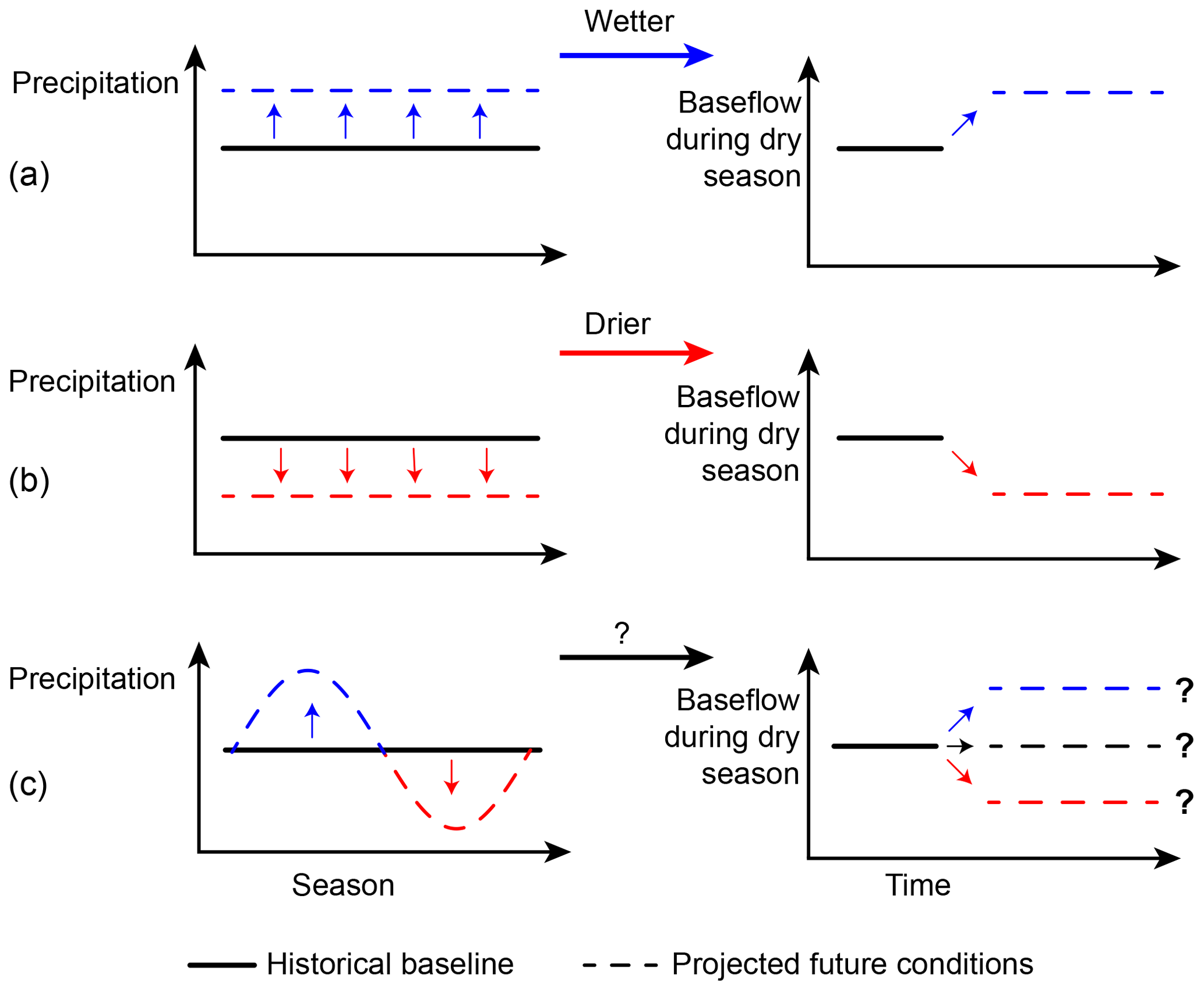
https://www.hydrol-earth-syst-sci.net/22/6209/2018/hess-22-6209-2018-f01

Figure 1Schematic direction of change of natural baseflow in the dry season under different climate change scenarios: (a) all seasons becoming wetter, (b) all seasons becoming drier and (c) seasonal shift of precipitation.

Download

For many parts of central Europe climate projections indicate a seasonal shift of precipitation to wetter winters and drier summers rather than a consistent increase/decrease (Jacob et al., 2014), urging for statistical tools to assess the prospective changes in baseflow. Knowledge of the seasonal to multi-annual scale of the baseflow response to climatic variation and extremes is therefore particularly important in central Europe under this seasonally diverging expected climate change.

This study aims to explain differences in drought trends by catchment characteristics to allow for more accurate predictions under climate projection uncertainty on a headwater scale. Firstly, past trends in baseflow drought and catchment-relevant response times are analysed. Secondly, past trends are attributed to climatic and catchment controls. Finally, based on these statistics an estimate for future changes in baseflow drought valid for all common emission scenarios and climate models is realized.

2 Study area and data

Back to toptop

The dataset used in this study is the same set of headwater catchments (that is, all catchment areas are below 200 km²) that were used in Hellwig et al. (2018) to evaluate the representativeness of meteorological grid data. It comprises streamflow data of daily resolution available from the responsible environment agencies of the German federal states. The lengths of available time series differ, so there is a trade-off between selected period and the number of records with sufficient data. For this study, we only used catchments with streamflow data of the period 1970 to 2009. Records with data gaps were not considered. Even though the dataset consists of near-natural headwaters with minimal regulations, the hydrographs and their double mass curves were visually screened for signs of anthropogenic influence. In a natural catchment under relatively constant conditions, the precipitation–streamflow relationship should be similar for the entire observation period. Four of the gauges showed sudden changes in the relationship and were subsequently removed. The final dataset consisted of 338 unnested and independent gauges across Germany (Fig. 2).

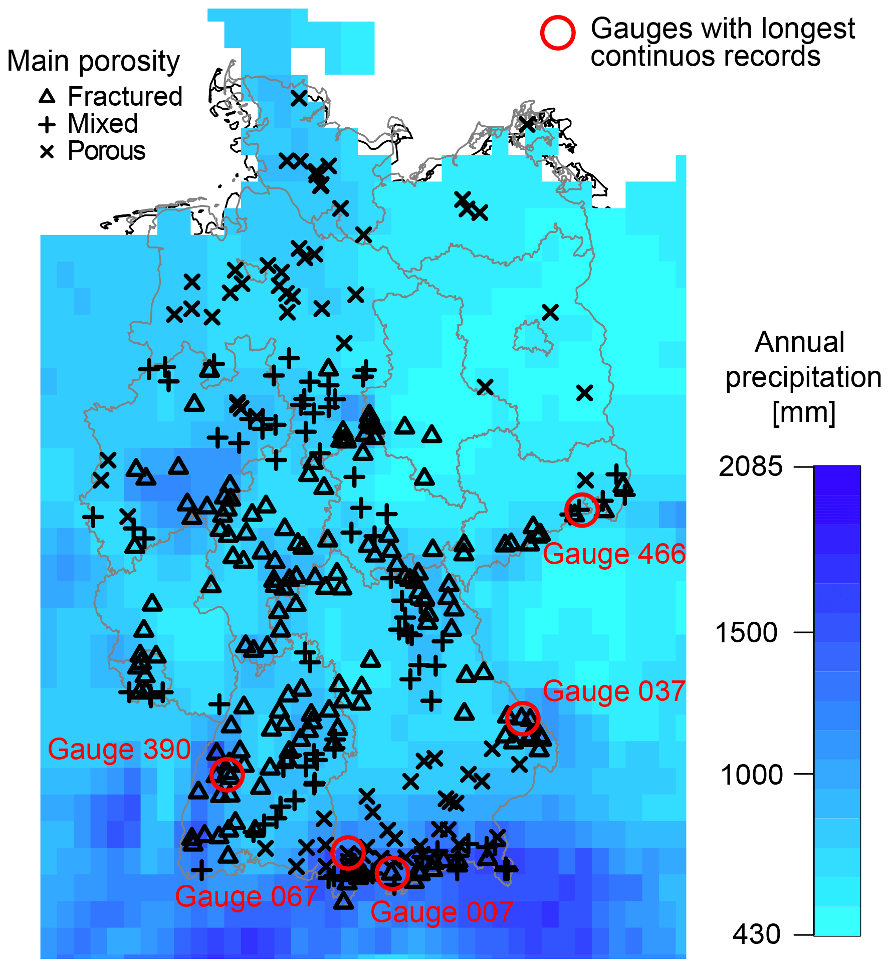
https://www.hydrol-earth-syst-sci.net/22/6209/2018/hess-22-6209-2018-f02

Figure 2Location of gauges in Germany, catchments' dominant type of porosity (derived from the German hydrogeological map) and mean annual precipitation sums (calculated from European Climate Assessment and Dataset E-OBS).

Download

The selected catchments cover the flat lowland regions in the north of Germany, the low mountain ranges in south-central Germany, and the Alpine foothills and non-glacierized front range in the south. Precipitation varies with highest annual precipitation sums in the Alpine south (> 2000 mm) and lowest sums in the northeast (< 500 mm). Climate in Germany is humid with slightly higher precipitation sums in summer than in winter for most regions. Precipitation was analysed in the form of monthly precipitation sums taken from the European Climate Assessment and Dataset (Haylock et al., 2008), Version 13.1. According to the procedure described in Hellwig et al. (2018), catchment-specific precipitation was calculated as an area-weighted mean of the intersecting grid cells. Hellwig et al. (2018) found that due to the low spatial resolution of the meteorological dataset compared to catchment size there are some biases towards products of higher resolution; however, correlations between products were found to be very high.

Information on the hydrogeology of the catchments was taken from the digital German hydrogeological map (Hydrogeologische Übersichtskarte von Deutschland 1:200.000, Oberer Grundwasserleiter; BGR and SGD, 2016). The catchments were classified according to the main type of porosity found in the underlying geology, either “porous” for porous aquifers such as unconsolidated alluvial and glacial fillings or “fractured” for fractured bedrock. Where less than two-thirds of the catchment's area is covered by one of these types, the class “mixed” was assigned, including catchments which are dominated by other types of porosity like karst. Additional analysis revealed that other reasonable thresholds for classifying the catchments do not change the results. According to this classification, 80 headwater catchments (23.7 %) are mainly “porous”, 170 catchments (50.3 %) are mainly “fractured” and 88 catchments (26.0 %) have “mixed” porosity (Fig. 2).

The dominant land use was derived from CORINE Land Cover 2006 data (available online from the German Environment Agency (https://www.umweltbundesamt.de, last access: 28 November 2018). Each catchment is classified as agricultural (53.6 %), urban (1.2 %) or forested (45.2 %).

To differentiate the catchments regarding topography, the average height above the catchment's outlet was calculated. This metric describes the potential groundwater waterbody that can contribute to the flow at the gauge and thus characterizes the potential storage. Elevation data (1 arcsec digital elevation model over Europe) were obtained from the European Environment Agency (2013).

3 Methods

Back to toptop

3.1 Characterizing baseflow drought

3.1.1 Baseflow as a measure of groundwater storage at the catchment scale

Baseflow Q_b is defined as the delayed component of streamflow Q, i.e. flow originating from stored sources as opposed to flow originating from event water (WMO, 2008). In groundwater-dominated catchments, where groundwater is the main water storage, Q_b is directly related to groundwater outflow (see Appendix A for a detailed rationale). Therefore, Q_b can be taken as an integrated measure of groundwater storage S as it was done in the study of Fendeková and Fendek (2012) and others. It is important to be aware that the unknown functional relationship between Q_b and S strongly differs between catchments and might be non-linear, e.g. due to temporal changes in connectivity of groundwater and surface water (Elthair and Yeh, 1999; Brunner et al., 2011). Hence, without further knowledge about this functional relationship, the observation of Q_b allows for conclusions about S solely on an ordinal scale.

Despite the clear concept of baseflow, there is no universally valid way to separate Q_b from time series of Q. Instead, a number of methods exist (e.g. WMO, 2008; Lyne and Hollick, 1979; Nathan and McMahon, 1990; Eckhardt, 2005; Mei and Anagnostou, 2015) that differ especially in baseflow estimation during high flow, when Q_b is relatively uncertain. For the type of extreme low-flow conditions considered in this study, most methods consistently assume that Q is almost completely comprised of Q_b. The World Meteorological Organization recommends a baseflow separation method (WMO, 2008) that was applied in this work using the package “lfstat” (Koffler et al., 2016) in the programming language R (R Core Team, 2016). The separation procedure consists of five steps: (i) divide the time series into non-overlapping blocks of a certain length N, where N is recommended to be 5 days for rainfall regimes which have a fast streamflow response; (ii) select the minimum value for every block; (iii) compare each minimum value with the adjacent ones (if the central value is a times smaller than the adjacent values, then it becomes a turning point; a is recommended to be 0.9 for rainfall regimes which have fast streamflow response); (iv) join the turning points by straight lines; and (v) compute the baseflow for every day by linearly interpolating between the turning points (if the computed value is higher than observed flow, use the observation instead).

3.1.2 Catchment-specific response times to precipitation

To quantify the catchments' baseflow response times to precipitation (T_R), time series of very different characteristics need to be related to each other. To enhance comparability over space, time and different parts of the hydrological cycle, it is common to standardize time series. Recent studies on drought have used either parametric (e.g. Fiorillo and Guadagno, 2012; Barker et al., 2016) or non-parametric approaches (e.g. Bloomfield and Marchant, 2013; Kumar et al., 2016) for standardization. Parametric approaches like the Standardized Precipitation Index (SPI), introduced by McKee et al. (1993), rely on the fitting of a theoretical distribution. Since time series of precipitation (P) and Q_b have distinct characteristics, entirely different distributions would have to be selected. To ensure consistency in the way of standardization, in this study a non-parametric approach was applied (Bloomfield and Marchant, 2013; Kumar et al., 2016). All time series (P in accumulation periods from 1 to 36 months, Q_b) were standardized according to the procedure of the Standardized Groundwater Index (SGI; Bloomfield and Marchant, 2013).

P (or Q_b) was transformed by using the inverse normal cumulative distribution function to calculate n equally spaced p_i values between 1∕(2n) and $1 - 1 / (2 n)$ , where n is the number of observations. These values were afterwards assigned to the time series by reordering them according to the ranks of the original time series. Hence, the ranks of the original time series and the new ones coincide, but the newly generated time series are normally distributed. Standardization was done separately for all 12 months of the year to account for the regime.

For all 338 catchments, correlation coefficients R between P and Q_b were calculated:

\begin{matrix} (1) & R = \frac{cov (x, y)}{σ_{x} σ_{y}} = cov (x y), \end{matrix}

where x and y are P and Q_b, respectively, with cov() the covariance and σ the standard deviation of each time series, which equals one for standardized time series. To derive the catchments' response times to precipitation, precipitation accumulation periods from 1 to 36 months were tested as well as time lags of these indices to baseflow from 0 to 10 months. For each catchment, the combination of precipitation accumulation period and time lag that has the highest correlation coefficient was selected as the optimal accumulation period and the optimal time lag to describe the Q_b response. Longer optimal accumulation periods indicate higher groundwater attenuation of precipitation input, whereas higher time lags represent a more delayed groundwater response to precipitation. To account for seasonal variations in the response times, correlations were calculated separately for all seasons (winter: DJF; spring: MAM; summer: JJA; autumn: SON).

3.1.3 Catchment-relevant recharge period

Catchments analysed in this study follow a distinct regime in Q_b. Thus, droughts in Q_b are most likely to occur in a certain period of the year. To derive the catchment-characteristic drought season, annual minimal 7-day Q_b (Q_b7) were calculated. The most frequent month of Q_b7 was assigned as the month of highest baseflow drought hazard ( $M_{Q_{b 7}}$ ). Subsequently, the derived seasonal T_R was used to determine the months influencing Q_b in $M_{Q_{b 7}}$ . For example, if $M_{Q_{b 7}}$ in a catchment was October and T_R for that catchment in autumn was 6 months, then the catchment-relevant recharge period would be May through October.

3.2 Detection of past baseflow drought trends

Time series of Q_b7 for the time period of 1970–2009 were used to analyse past trends in minimal baseflow. The analysis was carried out with the non-parametric Mann–Kendall (MK) test, which is a common tool used to detect monotonic increases or decreases in hydrological time series (e.g. used by Douglas et al., 2000; Lins and Slack, 1999; Lorenzo-Lacruz et al., 2012; Rennermalm et al., 2010; Asarian et al., 2016) and is robust to outliers. The test was performed after pre-whitening the time series to account for the influence of serial correlation (see Appendix B for calculation steps). A significance level of α=0.05 was used.

Trends only give information on the period they are calculated for. Many studies found that trends of a certain period are not part of a trend on another timescale (e.g. Stahl et al., 2010; Hannaford and Buys, 2012; Giuntoli et al., 2013; Hannaford et al., 2013). The analysis of trends for multiple periods may help to assess whether observed trends are steady or rather fluctuating. To evaluate the trends found for the period 1970–2009, we additionally calculated trends over multiple periods for the five gauges with longest continuous records. Three of these are in the porosity class “fractured”, and one each in “porous” and “mixed”.

3.3 Attribution of baseflow drought trends

Trends in Q_b7 were assumed to be driven by both climatic (climate control) and catchment-specific (catchment control) factors. Thus, the results were related to a set of potential predictors: (i) trends in P for the catchment-specific relevant recharge period, (ii) T_R for the catchment-specific $M_{Q_{b 7}}$ , (iii) $M_{Q_{b 7}}$ , (iv) dominant porosity of the catchment, (v) catchment size (A), (vi) dominant land use and (vii) potential storage. Statistical significance of the factors was determined using the correlation coefficient R (Eq. 1) for the continuous variables (trends in P, A, potential storage), Spearman's rank-based correlation coefficient for the discrete variable (T_R) and an analysis of variance (ANOVA) combined with the post hoc Tukey test (for details see Appendix C) for the nominally scaled ones ( $M_{Q_{b 7}}$ , dominant porosity, dominant land use).

3.4 Estimate of drought sensitivity to expected future precipitation change

Since past trends derived from empirical trend analysis (e.g. MK) are solely valid for the observation period, they cannot be extrapolated beyond the period of data availability. Future drought predictions therefore mostly rely on climate projections and process modelling. For Germany climate projections indicate little to no changes of annual precipitation sums but seasonal shifts to lower summer precipitation and higher winter precipitation. However, the magnitude of the shifts differs considerably for different projections (Zebisch et al., 2005; Jacob et al., 2012, 2014; Hübener et al., 2017). A common approach to dealing with such uncertainties is to use a range of possible trajectories to model hydrological change. Instead of using uncertain quantitative inputs in forward modelling, here we propose a more qualitative inverse approach. We assume that the general direction of future development is the most important piece of information for future groundwater management planning and formulate a qualitative test scenario of the consistent direction of different projections of future precipitation change. Thus, the approach is scenario-neutral regarding emission scenarios and climate models.

Trends in future baseflow drought hazard were assumed to depend not only on precipitation changes but also on T_R and $M_{Q_{b 7}}$ calculated for every catchment. A particular test scenario can still have three possible outcomes regarding future changes in baseflow drought hazard (Fig. 3): (i) increased baseflow – there are relevant months with increasing precipitation but not with decreasing precipitation; (ii) decreased baseflow – there are relevant months with decreasing precipitation but not with increasing precipitation; or (iii) no change – either there are relevant months with both increasing and decreasing precipitation or there are no relevant months with any change.

The test scenario applied in this study is a decrease of precipitation in summer (JJA) and an increase of precipitation in winter (DJF) with no change in the annual precipitation sum. To derive the future change in Q_b7 for a catchment, we analyse whether months with increasing or decreasing precipitation belong to the catchment-relevant recharge period. For example, for a catchment with a relevant recharge period from May to October we would estimate an increased baseflow drought hazard, since there are months with decreasing precipitation in the relevant recharge period (June, July and August) but no months with increasing precipitation. This analysis was carried out for all 338 catchments.

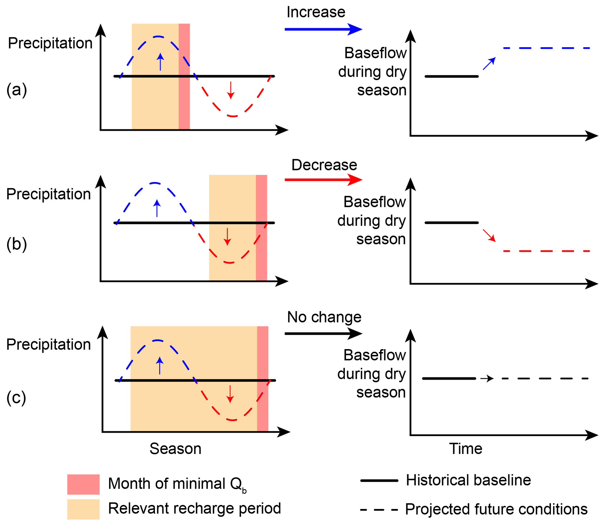
https://www.hydrol-earth-syst-sci.net/22/6209/2018/hess-22-6209-2018-f03

Figure 3Potential directional changes in Q_b7 under a constant seasonally diverging precipitation change scenario, depending on T_R and $M_{Q_{b 7}}$ : (a) increase, (b) decrease and (c) no change.

Download

4 Results

Back to toptop

4.1 Past minimal baseflow trends

$M_{Q_{b 7}}$ occurs in most parts of Germany in late summer or autumn with some exceptional winter low-flow catchments in the mountainous regions (Fig. 4). Seasonal response times vary across Germany, ranging from short subseasonal response times (1–3 months) to response times of over a year (Fig. 4b). Altogether 22 out of 338 catchments (∼6.5 %) have a time lag in the response, though these are mainly short. All five catchments with a time lag above 1 month have response times longer than 12 months. According to the MK test, 40 out of the 338 catchments show a significant trend of Q_b7 (Fig. 4c), corresponding to 11.8 %. Assuming independence of the baseflow observations, this is slightly more than the expected 5 % in case of no real trends. Hence, for the period of 1970–2009 there are some changes detectable for all catchments' porosity classes. For P there are even fewer significant trends than would be expected by chance (Fig. 4d). However, the results are skewed towards predominantly positive trends in P during the relevant recharge periods across Germany.

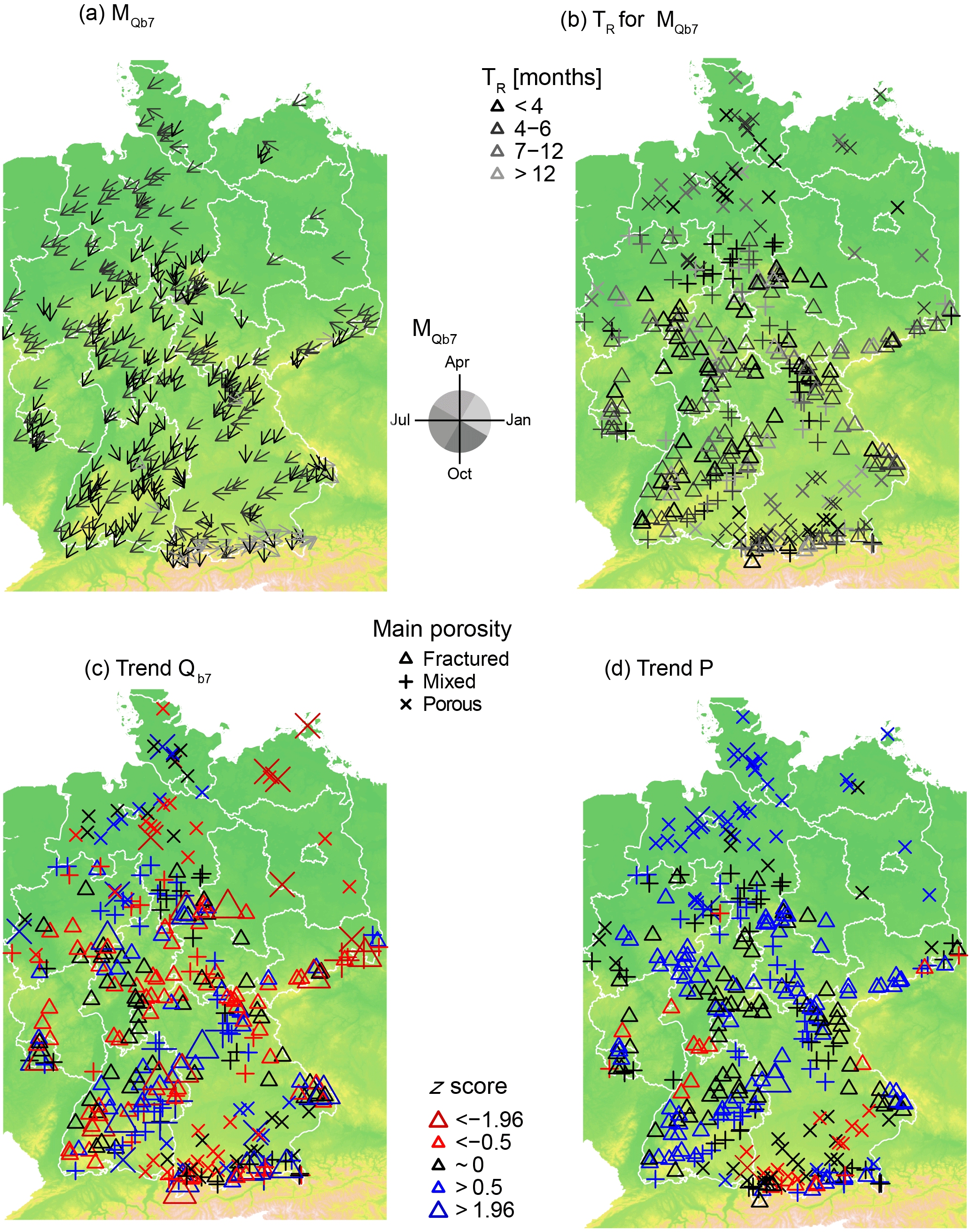
https://www.hydrol-earth-syst-sci.net/22/6209/2018/hess-22-6209-2018-f04

Figure 4Patterns of Q_b7 across Germany. (a) Low-flow month $M_{Q_{b 7}}$ and (b) seasonal response time T_R. (c) Trend of Q_b7 and (d) P in the relevant recharge period for 1970–2009.

Download

https://www.hydrol-earth-syst-sci.net/22/6209/2018/hess-22-6209-2018-f05

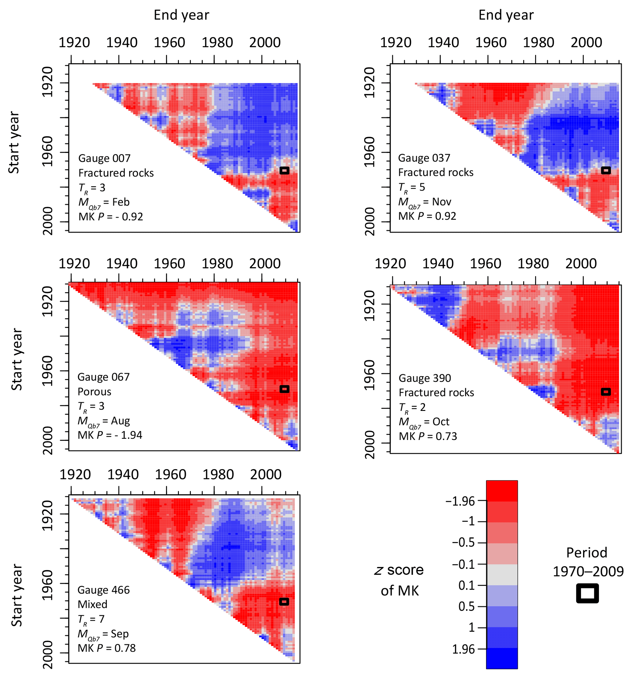
Figure 5z-score values for all possible periods for the five catchments with longest continuous records.

Download

The five selected gauges for a trend analysis on multiple periods all have a negative z score in the original period: 1970–2009 (Fig. 5). However, in all cases a significant positive trend could also have been observed if another period had been chosen for analysis (Fig. 5). This reveals a high influence of the observation period on the results of the trend analysis. The high variability of trends is also independent of the porosity, T_R and $M_{Q_{b 7}}$ .

4.2 Trend attribution

None of the factors tested was found to explain past trends of Q_b7 very well. This lack of statistical relation coincides with the results that few trends are significant and trend magnitude is highly dependent on the period of analysis. However, there is a small but significant correlation between the trends in P for the catchment-relevant recharge period and trends in Q_b7 (Fig. 6). Moreover, the ANOVA indicates a significant influence of $M_{Q_{b 7}}$ on the trends in Q_b7 even though Tukey's test does not distinguish two groups significantly. The largest differences are between July and November, so the season of low flow might be relevant for trend magnitude in Q_b7 as well. The remaining factors (T_R, dominant porosity, A, dominant land use and potential storage) do not show any relation to the trends in Q_b7 (Fig. 6).

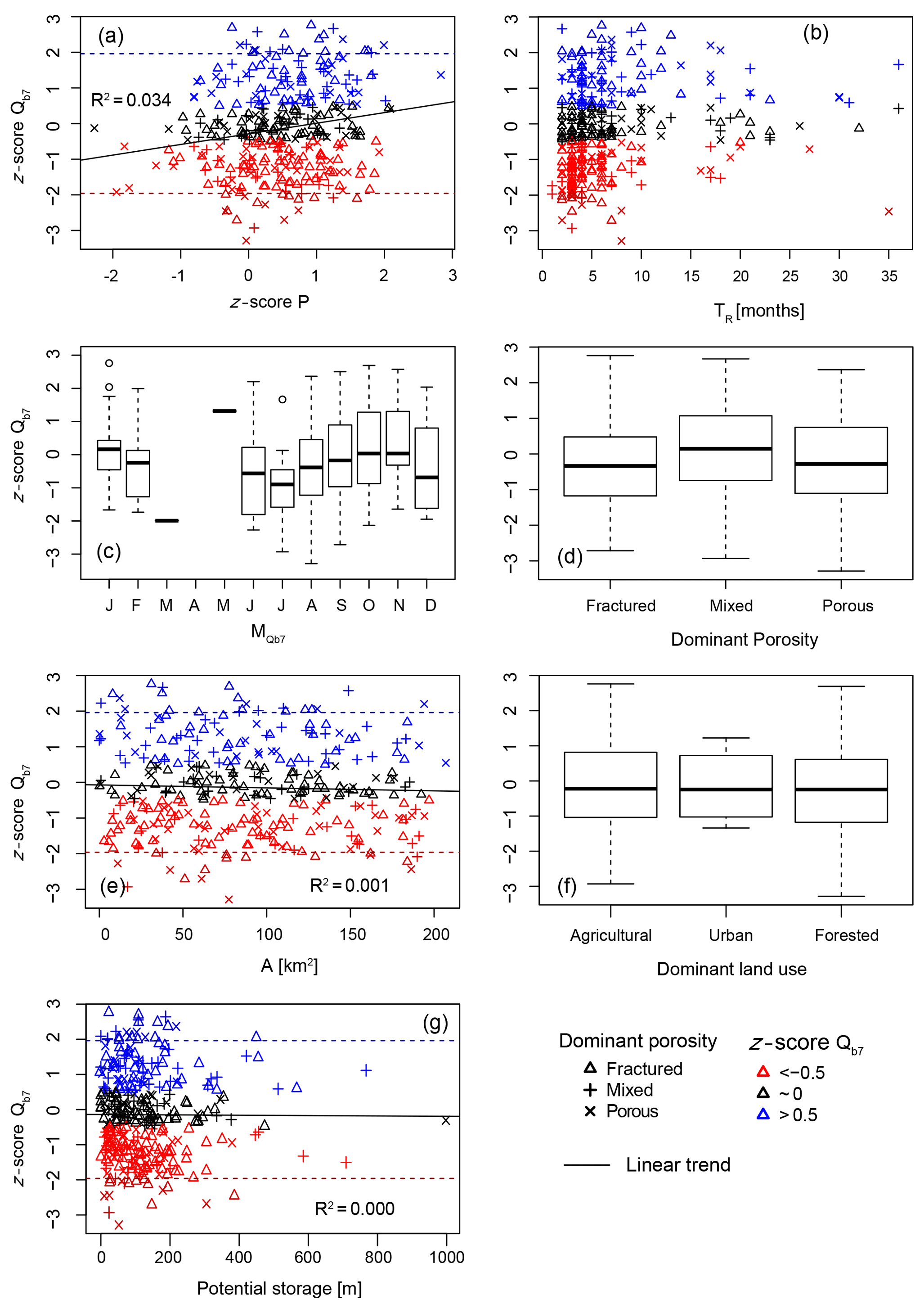
https://www.hydrol-earth-syst-sci.net/22/6209/2018/hess-22-6209-2018-f06

Figure 6Attribution of trends in Q_b7 to potential influencing factors. (a) Trends in precipitation P during the relevant recharge period, (b) length of response time T_R, (c) $M_{Q_{b 7}}$ , (d) dominant porosity in the catchment (e) catchment size A, (f) dominant land use in the catchment and (g) potential storage. Boxes represent the quartiles 0.25 and 0.75, and whiskers last to the most extreme value within a maximum distance of a 1.5-fold interquartile range.

Download

4.3 Potential future drought hazard

According to the test scenario, Q_b7 will decrease or not change for most of Germany (Fig. 7). The only catchments with estimated increases of Q_b7 are located in the mountainous regions of southeast Germany, especially in the Alpine foothills in the catchments with annual low flows in winter. However, in the catchments with annual low flows in winter or spring, impacts might also be more severe for low flows in summer or autumn. Additional tests revealed that, for 22 (27) out of 35 catchments with $M_{Q_{b 7}}$ in winter or spring, baseflows of the summer (autumn) season are expected to decrease according to the test scenario.

https://www.hydrol-earth-syst-sci.net/22/6209/2018/hess-22-6209-2018-f07

Figure 7Future changes in Q_b7 according to the test scenario.

Download

https://www.hydrol-earth-syst-sci.net/22/6209/2018/hess-22-6209-2018-f08

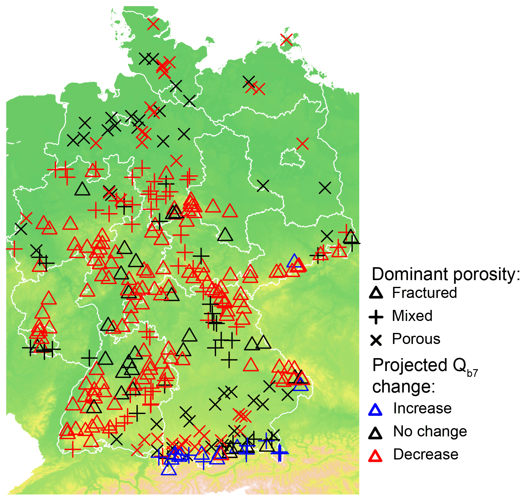
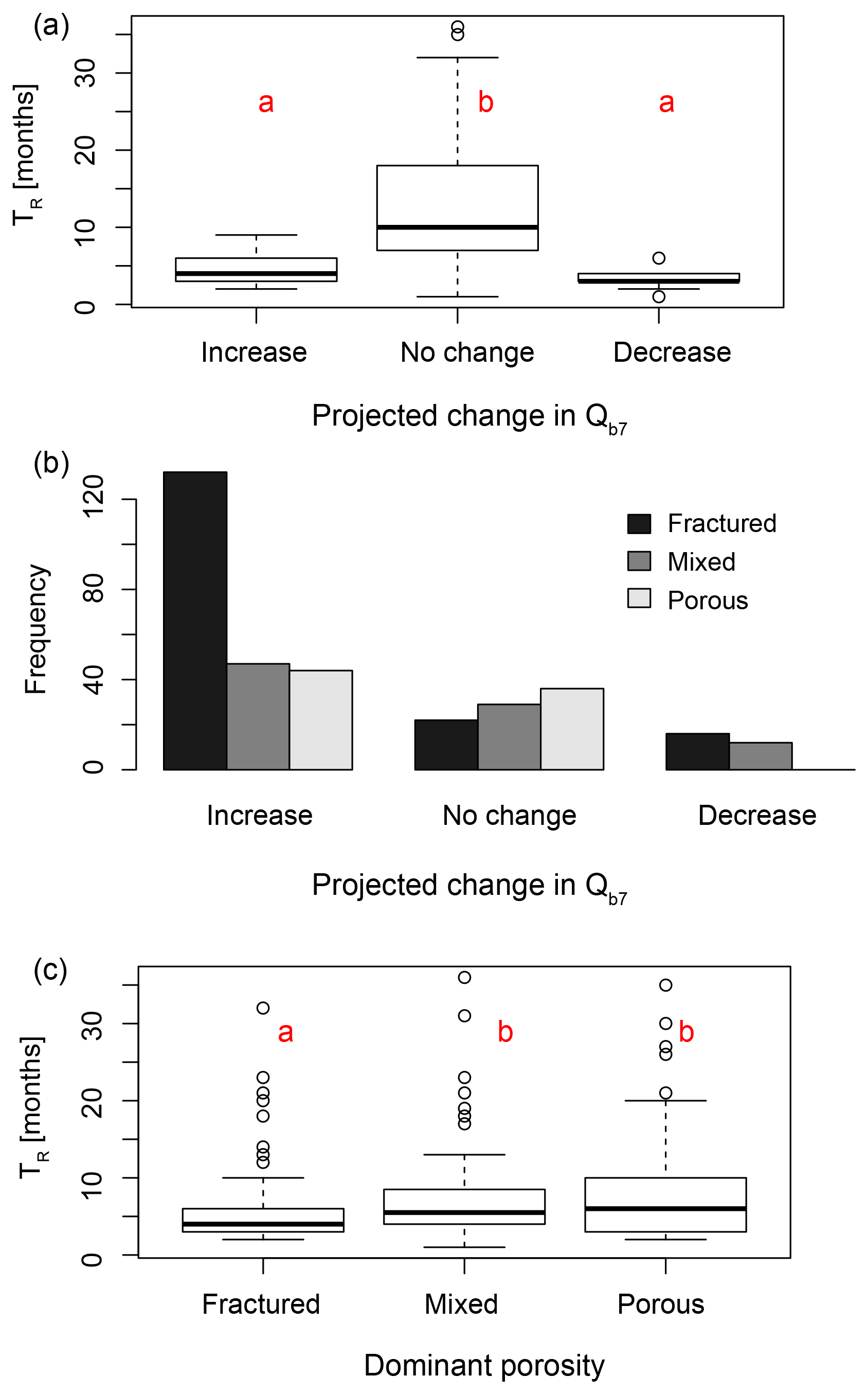
Figure 8Relationships of projected changes, T_R and catchment's dominant porosity. (a) Distribution of T_R for projected changes, (b) frequency of catchments with a certain dominant porosity for different projected changes and (c) distribution of T_R for dominant porosities. Boxes represent the quartiles 0.25 and 0.75, and whiskers last to the most extreme value within a maximum distance of a 1.5-fold interquartile range. Red letters indicate results of the post hoc Tukey test to distinguish significantly different groups.

Download

The changes in drought hazard are significantly related to the catchments' response times T_R (Fig. 8). Moreover, there is a strong statistical linkage to the dominant porosity (Fig. 8b). Catchments dominated by fractured rocks more frequently show estimated decreases in Q_b7 than the other classes. This coincides with a significant relationship between T_R and the dominant porosity of the catchment (Fig. 8c). According to Turkey's test, catchments with fractured rocks have shorter response times than the other classes. Contrarily, catchments with porous aquifers or mixed hydrogeology, which have long T_R, can more often compensate for summer precipitation decreases with winter increases and are therefore more frequently in the category “no change”.

5 Discussion

Back to toptop

5.1 The catchment baseflow response to precipitation

Catchments' response times to precipitation were found to be highly diverse across Germany, ranging from 1 month to 3 years. In general, baseflow response times determined as a proxy of groundwater response are rather short compared to other studies. Fiorillo and Guadagno (2012) found response times of 12 to 24 months for a karst region in southern Italy and highest correlations for shorter precipitation accumulation periods when adding a short time lag. Bloomfield and Marchant (2013) also found in 3 out of 14 cases a time lag for highest correlations. We found time lags to be an exception, supporting the results of Kumar et al. (2016), Barker et al. (2016) and Haas and Birk (2017). This indicates that, in the headwater catchments studied, the delay of the groundwater baseflow response to meteorological conditions may be shorter than 1 month and therefore not detectable on the monthly scale, whereas the attenuation of meteorological variability is clearly attributable to characteristic precipitation accumulation periods.

The large differences of baseflow response times for different porosity classes match the theoretical assumptions that baseflow strongly depends on hydrogeological conditions. For the entire streamflow, differences were found to be much smaller (not shown; compare e.g. Haslinger et al., 2014), since other processes like overland flow are also important. The patterns of T_R which are related to the catchments' hydrogeology support the assumption that baseflow can be used as a proxy of the groundwater situation on a catchment scale. More detailed information on hydrogeology has the potential to further improve the understanding of differences in baseflow response. However, this information is not yet detailed enough for the scale and distribution of headwater catchments. For example, two large-scale estimates on hydraulic conductivity available for Germany (GLHYMPS from Gleeson et al., 2014, and HÜK200 from BGR and SGD, 2016) were considered and found to differ up to 6 orders of magnitude. Moreover, information on superficial deposits that might be particularly important for streamflow generation could enhance results but is not available in detail yet.

Consistent with the work by Bloomfield et al. (2015), we found that hydrogeology is a highly relevant factor for the explanation of different groundwater baseflow response times. Kumar et al. (2016) did not find a relationship between the hydraulic conductivity and groundwater response time for boreholes. A possible reason for this different finding is that for point data even small local influences, which are hard to determine, are quite relevant (e.g. human influences), whereas baseflow reflects more the overall situation within the catchment. Small influences may be negligible at this scale, and the underlying influence of hydrogeology may be easier to detect.

In general, the results indicate that groundwater storage – represented by baseflow – is vitally driven by precipitation on a catchment scale in the relevant recharge period. However, the season of low flow is also expected to have an influence: regimes with winter low flows in central Europe are governed by snow storage during that season. Thus, not only precipitation but also temperature is a major factor for that catchments. Moreover, it is impossible to distinguish snowmelt from groundwater outflow during baseflow separation. Therefore, a baseflow approach does not allow for conclusions on groundwater storage in snow-dominated catchments.

5.2 Past and potential future changes in low baseflow

The trend analysis revealed that the trend in baseflow minima is highly dependent on the period it is calculated for. The observation of a trend in Q_b7 thus is a poor indicator of future developments. Despite the relatively narrow seasonality of low-baseflow timing (except for the alpine areas), trends are highly variable across the region – a result of the likewise variable response times. However, the correlation tests for attribution of the trends revealed that precipitation during the catchment-relevant recharge period is an important factor, which confirms previous model-based findings for part of the region (Stölzle et al., 2014). Thus, this catchment-relevant recharge period should be considered for projections.

The method employed in this study provides a straightforward projection of the probable future directions of changes in baseflow or groundwater drought under climate change. We accounted for the uncertainty in future climate projections by taking only concordant directions of precipitation change in our approach. Contrary to future climate projections, past trends in precipitation for the catchment-relevant recharge period were found to be small and mostly positive. Similarly, Kopp et al. (2018) found for southern Germany a high variability of annual groundwater recharge without distinct trends. In the past, precipitation trends have not been seasonally diverging, but climate models suggest that changes will become more relevant in the second half of this century (e.g. Jacob et al., 2012). As the magnitude of the trends differs for the climate models, we did not quantify our scenario and thus did not quantify the magnitude of future baseflow either.

Catchments' characteristic response times were assumed to remain constant. Under a more extreme climate change however, changes in catchments' responses (e.g. due to non-stationary response times) cannot be excluded. Based on assumed precipitation change in the catchments' respective recharge periods, decreasing Q_b7 (i.e. increased groundwater drought hazard) were estimated for the majority of the catchments. This is because of the timing of $M_{Q_{b 7}}$ , which occurs predominantly in summer/autumn. Only those catchments with long response times can compensate for the decreases in summer precipitation, and only in the Alpine foothills, where $M_{Q_{b 7}}$ is in winter, is a decrease in drought hazard predicted. However, in this region winter precipitation is mainly snow and therefore does not immediately contribute to groundwater recharge. Moreover, air temperature and its changes over time – which are not considered in the test scenario – are especially important for winter low flows. Hence, uncertainty is quite high for these projections. If response times are not assumed constant, further conclusions may be drawn. A decrease of response times might be caused by decreased storage, e.g. due to urbanization, or accelerated drying and increased evapotranspiration in spring. Such changes would increase the drought hazard for most parts of Germany due to the timing of $M_{Q_{b 7}}$ . An increase in response times by the opposite processes is possibly less likely but could compensate for the reduced precipitation during summer for the catchments that are currently estimated to have increased drought hazard.

6 Conclusions

Back to toptop

Climate change is expected to alter the hydrological drought hazard. However, uncertainty of climate projections and even contrasting seasonal changes impede a straightforward assessment of the prospective changes in central Europe and elsewhere. Here we presented a statistical approach to estimating the potential direction of future changes in hydrological drought hazard. Past trends were found to be too variable to provide a consistent regional picture of past and expected changes because of their high dependency on the trend calculation period. But they did allow the attribution of trends in baseflow to precipitation changes in catchment-specific recharge periods. Based on that information, a more process-oriented approach was developed, using the catchments' characteristic response times to precipitation and the relevant recharge periods for projections valid for all common emission scenarios and climate models. These projections are efficient alternatives to ensemble projections and target the most important information for management. Especially for regions where directions of climate change are seasonally varying, they can provide valuable insights into the basic changes of the system.

Catchments with short response times were found to have a high probability for a decrease in baseflow minima and hence an increase in the groundwater drought hazard, as seasonal changes cannot compensate for each other. However, there is no homogeneous pattern of response times across central Europe, and so predicted changes of groundwater drought hazard also vary regionally. This urges for a regionally adapted groundwater management based on the local catchment response times. As past events like the 2015 central European drought have already caused groundwater-related drought impacts in headwater regions, there is an urgent need for adaptation in catchments facing even higher drought hazard in the future.

The diversity of response times, the dearth of long-time data on groundwater storage, and the absence of distinct past trends in precipitation and hydrological variables limit the potential to generalize the results. On the path to extensive predictions of future groundwater drought hazard across central Europe, further model-based work will be needed. Reproducing the catchment-relevant response times with high-resolution large-scale models may be key for an assessment of future changes and related implications for groundwater management under various scenarios and for ungauged catchments.

Data availability

Back to toptop

Data availability.

Streamflow data are available on request for scientific purposes from the responsible federal state agencies, i.e. the State Environmental Agency of Baden-Württemberg, Bavaria, Brandenburg, Hesse, Mecklenburg-Western Pomerania, Lower Saxony, North Rhine-Westphalia, Rhineland-Palatinate, Saarland, Saxony, Saxony-Anhalt, Schleswig-Holstein and Thuringia. Climate data are available via the website of the European Climate Assessment and Dataset (https://www.ecad.eu/, ECA and D, 2018); the German hydrogeological map (BGR & SGD, 2016) is online available as well (https://www.bgr.bund.de/DE/Themen/Wasser/Projekte/laufend/Beratung/Huek200/huek200_projektbeschr.html, Bundesanstalt für Geowissenschaften und Rohstoffe, 2018).

Appendix A: Mathematical relationship between baseflow and groundwater storage

Back to toptop

In groundwater-dominated catchments Q_b is an integrated signal of groundwater conditions in the entire area and mainly depends as a function g on the hydraulic head H of the groundwater:

\begin{matrix} (A1) & Q_{b} = g (H) + r with \frac{d Q_{b}}{d H} > 0 \forall H, \end{matrix}

where r is the additional flow from other stored sources. H is a monotonic function f of groundwater storage S:

\begin{matrix} (A2) & H = f (S) with \frac{d H}{d S} > 0 \forall S . \end{matrix}

Combining Eqs. (A1) and (A2) leads to

\begin{matrix} (A3) & Q_{b} = g (f (S)) + r = k (S) + r with \frac{d Q_{b}}{d S} > 0 \forall S . \end{matrix}

Because of the monotonic behaviour, function k is reversible:

\begin{matrix} (A4) & S = k^{- 1} (Q_{b} - r) with \frac{d S}{d (Q_{b} - r)} > 0 \forall Q_{b} - r . \end{matrix}

Potential sources for r include snowmelt, interflow, lake outflow, sewage discharge or other anthropogenic sources of discharge. Anthropogenic influences can be assumed negligible, as catchments in this study were selected as near-natural. Moreover, there are no big lakes or other surface water storages in the catchments. Snowmelt remains an important factor that might blur the true signal of groundwater storage. This is particularly important for the catchments at higher elevations, e.g. in the Alps, and must be considered for the interpretation of the results. However, in catchments where these factors are of minor relevance compared to groundwater outflow, Eq. (A4) simplifies to

\begin{matrix} (A5) & S ≃ k^{- 1} (Q_{b}) with \frac{d S}{d (Q_{b})} > 0 \forall Q_{b}; \end{matrix}

i.e. higher baseflow indicates higher groundwater storage, and vice versa. However, without further knowledge about k⁻¹, the observation of Q_b allows for conclusions about S solely on an ordinal scale.

Appendix B: The Mann–Kendall trend test with pre-whitening

Back to toptop

To calculate trends, the non-parametric Mann–Kendall (MK) test was applied. However, the results are affected by serial correlation which increases the type I error (i.e. rejecting the no-trend hypothesis although there is no trend). To test for serial correlation in the data, we fitted an autocorrelation AR(1) model to each Q_b7 time series. The calculated autocorrelation is significant on a level of α=0.05 if absolute autocorrelation is higher than $1.96 / \sqrt n$ (Douglas et al., 2000), where n is the length of the time series (in this case n=40). One hundred thirty (130) out of 338 time series showed significant serial correlation, thus requiring a pre-processing before using MK. Kulkarni and Von Storch (1995) recommended pre-whitening time series to allow for the MK. Since the sample size is relatively small here and trend magnitude not too large, pre-whitening is not expected to reduce the MK test power much in this case, but rather to reduce the type I error (Bayazit and Önöz, 2007). Pre-whitening was done according to other studies (Kulkarni and Von Storch, 1995; Douglas et al., 2000) as in Eq. (A6):

\begin{matrix} (B1) & Y_{t} = X_{t} - r_{1} X_{t - 1}, \end{matrix}

where Y_t is the pre-whitened time series at time step t, X_t is the original time series at time step t and r₁ is the serial correlation determined with the AR(1) model. Pre-whitening reduced the serial correlation in all time series to close to zero.

The MK test compares the number of concordant pairs in the data with the number of discordant pairs. This gives the Kendall score S_K (Kendall, 1948):

\begin{matrix} (B2) & S_{K} = \sum_{j > i} sign (Y_{j} - Y_{i}) sign (Z_{j} - Z_{i}), \end{matrix}

where sign() is a function that returns the algebraic sign. For the Mann–Kendall trend test that was applied here, Z is time. Therefore, the second part of Eq. (A7) always equals +1, and it simplifies to

\begin{matrix} (B3) & S_{K} = \sum_{j > i} sign (Y_{j} - Y_{i}) . \end{matrix}

In the case of no real trend, S_K has a mean value of zero; in the case of no ties in the data, it has a standard deviation σ_S of (Kendall, 1948)

\begin{matrix} (B4) & σ_{S} = \sqrt{\frac{n (n - 1) (2 n + 5)}{18}} . \end{matrix}

Thus, S_K can be transformed into the standard normal distributed z score by dividing by the standard deviation of S_K:

\begin{matrix} (B5) & z = \{\begin{cases} \frac{S_{K} - 1}{σ_{S}} if S_{K} > 0 \\ 0 if S_{K} = 0 \\ \frac{S_{K} + 1}{σ_{S}} if S_{K} < 0 \end{cases} . \end{matrix}

z was assumed to be significant if it was not within the interval ±1.96, i.e. a significance level of α=0.05.

Appendix C: ANOVA and Tukey's test

Back to toptop

To detect the influence of a categorical variable with multiple levels on a numerical variable, an ANOVA was used in this work. The ANOVA compares S_e, the sum of squares explained by the categorical variable's levels, with the sum of squares of the residuals (S_r). The mean sums (M_Se, M_Sr) are tested for significance using the F test:

\begin{matrix} (C1) & F = \frac{M_{Se}}{M_{Sr}} = \frac{S_{e} / d_{fe}}{S_{r} / d_{fr}}, \end{matrix}

where d_f denotes the degrees of freedom (d_fe: number of levels minus 1; d_fr: amount of data minus d_fe minus 1). The test statistic F follows the F distribution and was assumed to be significant for p < 0.05.

The ANOVA gives information about the general significance of the categorical variable. An equally important piece of information is which of the categorical variable's levels differ significantly regarding the target variable. This information was obtained using the post hoc Tukey test. For this analysis a pairwise t test between all levels is carried out:

\begin{matrix} (C2) & t = \frac{{\overline{x}}_{1} - {\overline{x}}_{2}}{\sqrt{\frac{s_{1}^{2}}{n_{1}} - \frac{s_{2}^{2}}{n_{2}}}}, \end{matrix}

where ${\overline{x}}_{i}$ and $s_{i}^{2}$ are the mean and the variance for the two levels, respectively, and n_i is the amount of data per level. Tukey's test accounts for the multiple-comparison problem (i.e. a higher probability of getting significant results by chance due to a higher number of comparisons) by using the studentized range distribution instead of the t distribution. Again, the results were assumed to be significant for p< 0.05.

Author contributions

Back to toptop

Author contributions.

JH and KS designed the study. JH performed all analyses and prepared the manuscript. Both authors revised the manuscript and approved the final version.

Competing interests

Back to toptop

Competing interests.

The authors declare that they have no conflict of interest.

Acknowledgements

Back to toptop

Acknowledgements.

We acknowledge the data providers at the federal states' agencies for the streamflow data, the E-OBS dataset from the EU-FP6 project ENSEMBLES (https://ensembles-eu.metoffice.com, last access: 28 November 2018) and the data providers in the ECA&D project (https://www.ecad.eu, last access: 28 November 2018). The authors were funded by the DFG (Jost Hellwig: project TrenDHy DFG STA632/4-1; Kerstin Stahl: Heisenberg programme STA632/3-1). Benedikt Heudorfer provided helpful comments on the manuscript. We are grateful for the comments of John Bloomfield and Spencer Sawaske, which helped to improve the quality of the manuscript. The article processing charge was funded by the German Research Foundation (DFG) and the University of Freiburg in the funding programme Open Access Publishing. Edited by: Stacey Archfield Reviewed by: John Bloomfield and Spencer Sawaske

References

Back to toptop

Apurv, T., Sivapalan, M., and Cai, X: Understanding the Role of Climate Characteristics in Drought Propagation, Water Resour. Res., 53, 9304–9329, https://doi.org/10.1002/2017WR021445, 2017.

Asarian, J. E. and Walker, J. D.: Long term trends in streamflow and precipitation in northwest California and southwest Oregon, 1953–2012, J. Am. Water. Resour. As., 52, 241–261, https://doi.org/10.1111/1752-1688.12381, 2016.

Barker, L. J., Hannaford, J., Chiverton, A., and Svensson, C.: From meteorological to hydrological drought using standardised indicators, Hydrol. Earth Syst. Sci., 20, 2483–2505, https://doi.org/10.5194/hess-20-2483-2016, 2016.

Bayazit, M. and Önöz, B.: To prewhiten or not to prewhiten in trend analysis? Hydrolog. Sci. J., 52, 611–624, https://doi.org/10.1623/hysj.52.4.611, 2007.

BGR and SGD: Bundesanstalt für Geowissenschaften und Rohstoffe and Staatliche Geologische Dienste: Hydrogeologische Übersichtskarte von Deutschland 1:200.000, Oberer Grundwasserleiter (HÜK200 OGWL), Digitaler Datenbestand, Version 3.0. – Hannover, 2016.

Bloomfield, J. P. and Marchant, B. P.: Analysis of groundwater drought building on the standardised precipitation index approach, Hydrol. Earth Syst. Sci., 17, 4769–4787, https://doi.org/10.5194/hess-17-4769-2013, 2013.

Bloomfield, J. P., Marchant, B. P., Bricker, S. H., and Morgan, R. B.: Regional analysis of groundwater droughts using hydrograph classification, Hydrol. Earth Syst. Sci., 19, 4327–4344, https://doi.org/10.5194/hess-19-4327-2015, 2015.

Bundesanstalt für Geowissenschaften und Rohstoffe: HÜK200 – Hydrogeologische Übersichtskarte von Deutschland 1:200 000, available at: https://www.bgr.bund.de/DE/Themen/Wasser/Projekte/laufend/Beratung/Huek200/huek200_projektbeschr.html, last access: 28 November 2018.

Brunner, P., Cook, P. G., and Simmons, C. T.: Disconnected Surface Water and Groundwater: From Theory to Practice, Ground Water, 49, 460–467, https://doi.org/10.1111/j.1745-6584.2010.00752.x, 2011.

Brutsaert, W.: Long-term groundwater storage trends estimated from streamflow records: Climatic perspective, Water Resour. Res., 44, W02409, https://doi.org/10.1029/2007wr006518, 2008.

Brutsaert, W.: Annual drought flow and groundwater storage trends in the eastern half of the United States during the past two-third century, Theor. Appl. Climatol., 100, 93–103, https://doi.org/10.1007/s00704-009-0180-3, 2010.

Douglas, E. M., Vogel, R. M., and Kroll, C. N.: Trends in floods and low flows in the United States: impact of spatial correlation, J. Hydrol., 240, 90–105, https://doi.org/10.1016/s0022-1694(00)00336-x, 2000.

EC: Communication from the Commission to the European Parliament and the Council addressing the challenge of water scarcity and droughts in the European Union, Commission of the European Communities, COM(2007), 414 final, Brussels, 2007.

ECA and D: European Climate Assessment & Dataset, available at: https://www.ecad.eu/, last access: 28 November 2018.

Eckhardt, K.: How to construct recursive digital filters for baseflow separation, Hydrol. Process., 19, 507–515, https://doi.org/10.1002/hyp.5675, 2005.

Eltahir, E. A. B. and Yeh, P.: On the asymmetric response of aquifer water level to floods and droughts in Illinois, Water Resour. Res., 35, 1199–1217, https://doi.org/10.1029/1998wr900071, 1999.

European Environment Agency: Digital Elevation Model over Europe (EU-DEM), available at: https://www.eea.europa.eu/data-and-maps/data/eu-dem (last access: 28 November 2018), 2013.

Fendeková, M. and Fendek, M.: Groundwater drought in the Nitra river basin-identification and classification, J. Hydrol. Hydromech., 60, 185–193, 2012.

Fiorillo, F. and Guadagno, F. M.: Long karst spring discharge time series and droughts occurrence in Southern Italy, Environ. Earth Sci., 65, 2273–2283, 2012.

Forzieri, G., Feyen, L., Rojas, R., Flörke, M., Wimmer, F., and Bianchi, A.: Ensemble projections of future streamflow droughts in Europe, Hydrol. Earth Syst. Sci., 18, 85–108, https://doi.org/10.5194/hess-18-85-2014, 2014.

Giuntoli, I., Renard, B., Vidal, J. P., and Bard, A.: Low flows in France and their relationship to large-scale climate indices, J. Hydrol., 482, 105–118, https://doi.org/10.1016/j.jhydrol.2012.12.038, 2013.

Gleeson, T., Moosdorf, N. Hartmann, J., and van Beek L. P. H.: A glimpse beneath earth's surface: Global HYdrogeology MaPS (GLHYMPS) of permeability and porosity, Geophys. Res. Lett., 41, 3891–3898, https://doi.org/10.1002/2014GL059856, 2014.

Gosling, S. N., Zaherpour, J., Mount, N. J., Hattermann, F. F., Dankers, R., Arheimer, B., Breuer, L., Ding, J., Haddeland, I., Kumar, R., Kundu, D., Liu, J., Van Griensven, A., Veldkamp, T. I. E., Vetter, T., Wang, X., and Zhang, X. X.: A comparison of changes in river runoff from multiple global and catchment-scale hydrological models under global warming scenarios of 1 degrees C, 2 degrees C and 3 degrees C, Clim. Change, 141, 577–595, https://doi.org/10.1007/s10584-016-1773-3, 2017.

Green, T. R., Taniguchi, M., Kooi, H., Gurdak, J. J., Allen, D. M., Hiscock, K. M., Treidel, H., and Aureli, A.: Beneath the surface of global change: Impacts of climate change on groundwater, J. Hydrol., 405, 532–560, https://doi.org/10.1016/j.jhydrol.2011.05.002, 2011.

Haas, J. C. and Birk, S.: Characterizing the spatiotemporal variability of groundwater levels of alluvial aquifers in different settings using drought indices, Hydrol. Earth Syst. Sci., 21, 2421–2448, https://doi.org/10.5194/hess-21-2421-2017, 2017.

Hannaford, J. and Buys, G.: Trends in seasonal river flow regimes in the UK, J. Hydrol., 475, 158–174, https://doi.org/10.1016/j.jhydrol.2012.09.044, 2012.

Hannaford, J., Buys, G., Stahl, K., and Tallaksen, L. M.: The influence of decadal-scale variability on trends in long European streamflow records, Hydrol. Earth Syst. Sci., 17, 2717–2733, https://doi.org/10.5194/hess-17-2717-2013, 2013.

Haslinger, K., Koffler, D., Schoner, W., and Laaha, G.: Exploring the link between meteorological drought and streamflow: Effects of climate- catchment interaction, Water Resour. Res., 50, 2468–2487, https://doi.org/10.1002/2013wr015051, 2014.

Haylock, M. R., Hofstra, N., Tank, A., Klok, E. J., Jones, P. D., and New, M.: A European daily high-resolution gridded data set of surface temperature and precipitation for 1950–2006, J. Geophys. Res.-Atmos., 113, D20119, https://doi.org/10.1029/2008jd010201, 2008.

Hellwig, J., Stahl, K., Ziese, M., and Becker, A.: The impact of the resolution of meteorological data sets on catchment-scale precipitation and drought studies, Int. J. Climatol., 38, 3069–3081, https://doi.org/10.1002/joc.5483, 2018.

Heudorfer, B. and Stahl, K: Comparison of different threshold level methods for drought propagation analysis in Germany, Hydrol. Res., 48, 1311–1326, https://doi.org/10.2166/nh.2016.258, 2017.

Hübener, H., Bülow, K., Fooken, C., Früh, B, Hoffmann, P, Höpp, S., Keuler, K., Menz, C., Mohr, V., Radtke K., Ramthun, H., Spekat, A., Steger, C., Toussaint, F., Warrach-Sagi, K., and Woldt, M. ReKliEs-De, Ergebnisbericht, HLNUG, Hessisches Landesamt für Naturschutz, Umwelt und Geologie, 2017.

Jacob, D., Bülow, K., Kotova, L., Moseley, C., Petersen, J., and Rechid, D.: Regionale Klimaprojektionen für Europa und Deutschland: Ensemble Simulationen für die Klimafolgenforschung, MPI für Meteorologie, Climate Service Center, 2012.

Jacob, D., Petersen, J., Eggert, B., Alias, A., Christensen, O. B., Bouwer, L. M., Braun, A., Colette, A., Déqué, M., Georgievski, G., Georgopoulou, E., Gobiet, A., Menut, L., Nikulin, G., Haensler, A., Hempelmann, N., Jones, C., Keuler, K., Kovats, S., Kröner, N., Kotlarski, S., Kriegsmann, A., Martin, E., Van Meijgaard, E., Moseley, C., Pfeifer, S., Preuschmann, S., Radermacher, C., Radtke, K., Rechid, D., Rounsevell, M., Samuelsson, P., Somot, S., Soussana, J.-F., Teichmann, C., Valentini, R., Vautard, R., Weber, B., and Yiou, P.: EURO-CORDEX: new high-resolution climate change projections for European impact research, Reg. Environ. Change, 14, 563–578, https://doi.org/10.1007/s10113-013-0499-2, 2014.

Kendall, M. G.: Rank correlation methods, London: Griffin, 160 pp., 1948.

Koffler, D., Gauster, T., and Laaha, G.: lfstat: Calculation of Low Flow Statistics for Daily Stream Flow Data. R package version 0.9.4. available at: https://CRAN.R-project.org/package=lfstat (last access: 28 November 2018), 2016.

Kulkarni, A. and von Storch, H.: Monte Carlo experiments on the effect of serial correlation on the Mann-Kendall test of trend, Meteorol. Z., 4, 82–85, 1995.

Kopp, B., Baumeister, C., Gudera, T., Hergesell, J., Morhard, A., and Neumann, J.: Entwicklung von Bodenwasserhaushalt und Grundwasserneubildung in Baden-Württemberg, Bayern, Rheinland-Pfalz und Hessen von 1951 bis 2015, Hydrol. Wasserbewirts., 62, 62–76, https://doi.org/10.5675/HyWa_2018,2_1, 2018.

Kumar, R., Musuuza, J. L., Van Loon, A. F., Teuling, A. J., Barthel, R., Ten Broek, J., Mai, J., Samaniego, L., and Attinger, S.: Multiscale evaluation of the Standardized Precipitation Index as a groundwater drought indicator, Hydrol. Earth Syst. Sci., 20, 1117–1131, https://doi.org/10.5194/hess-20-1117-2016, 2016.

Laaha, G., Gauster, T., Tallaksen, L. M., Vidal, J.-P., Stahl, K., Prudhomme, C., Heudorfer, B., Vlnas, R., Ionita, M., Van Lanen, H. A. J., Adler, M.-J., Caillouet, L., Delus, C., Fendekova, M., Gailliez, S., Hannaford, J., Kingston, D., Van Loon, A. F., Mediero, L., Osuch, M., Romanowicz, R., Sauquet, E., Stagge, J. H., and Wong, W. K.: The European 2015 drought from a hydrological perspective, Hydrol. Earth Syst. Sci., 21, 3001–3024, https://doi.org/10.5194/hess-21-3001-2017, 2017.

Leelaruban, N., Padmanabhan, G., and Oduor, P.: Examining the Relationship between Drought Indices and Groundwater Levels, Water, 9, 82, https://doi.org/10.3390/w9020082, 2017.

Li, B. and Rodell, M.: Evaluation of a model-based groundwater drought indicator in the conterminous US, J. Hydrol., 526, 78–88, https://doi.org/10.1016/j.jhydrol.2014.09.027 2015.

Lins, H. F. and Slack, J. R.: Streamflow trends in the United States, Geophys. Res. Lett., 26, 227–230, https://doi.org/10.1029/1998gl900291, 1999.

Lorenzo-Lacruz, J., Vicente-Serrano, S. M., López-Moreno, J. I., Morán-Tejeda, E., and Zabalza, J.: Recent trends in Iberian streamflows (1945–2005), J. Hydrol., 414, 463–475, https://doi.org/10.1016/j.jhydrol.2011.11.023, 2012.

Lyne, V. and Hollick, M.: Stochastic time-variable rainfall-runoff modelling, Paper presented at the Institute of Engineers Australia National Conference, Perth, Australia, 1979.

Marx, A., Kumar, R., Thober, S., Rakovec, O., Wanders, N., Zink, M., Wood, E. F., Pan, M., Sheffield, J., and Samaniego, L.: Climate change alters low flows in Europe under global warming of 1.5, 2, and 3 ^∘C, Hydrol. Earth Syst. Sci., 22, 1017–1032, https://doi.org/10.5194/hess-22-1017-2018, 2018.

McKee, T. B., Doesken, N., J., and Kleist, J.: The relationship of drought frequency and duration to time scales. Eighth Conference on Applied Climatology, Anaheim CA, 6, 1993.

Mei, Y. and Anagnostou, E. N.: A hydrograph separation method based on information from rainfall and runoff records, J. Hydrol., 523, 636–649, https://doi.org/10.1016/j.jhydrol.2015.01.083, 2015.

Mishra, A. K. and Singh, V. P.: A review of drought concepts, J. Hydrol., 391, 204–216, https://doi.org/10.1016/j.jhydrol.2010.07.012, 2010.

Nathan, R. J. and McMahon, T. A.: Evaluation of automated techniques for base flow and recession analyses, Water Resour. Res., 26, 1465–1473, 1990.

Peters, E., Torfs, P., van Lanen, H. A. J., and Bier, G.: Propagation of drought through groundwater – a new approach using linear reservoir theory, Hydrol. Process., 17, 3023–3040, https://doi.org/10.1002/hyp.1274, 2003.

Peters, E., Bier, G., van Lanen, H. A. J., and Torfs, P.: Propagation and spatial distribution of drought in a groundwater catchment, J. Hydrol., 321, 257–275, https://doi.org/10.1016/j.jhydrol.2005.08.004, 2006.

R Core Team: R: A language and environment for statistical computing. R Foundation for Statistical Computing, Vienna, Austria, available at: https://www.R-project.org/ (last access: 28 November 2018), 2016.

Rennermalm, A. K., Wood, E. F., and Troy, T. J.: Observed changes in pan-arctic cold-season minimum monthly river discharge, Clim. Dynam., 35, 923–939, https://doi.org/10.1007/s00382-009-0730-5, 2010.

Sheffield, J., Wood, E. F., and Roderick, M. L.: Little change in global drought over the past 60 years, Nature, 491, 435–438, 2012.

Spinoni, J., Naumann, G., and Vogt, J. V.: Pan-European seasonal trends and recent changes of drought frequency and severity, Global Planet. Change, 148, 113–130, https://doi.org/10.1016/j.gloplacha.2016.11.013, 2017.

Stahl, K., Hisdal, H., Hannaford, J., Tallaksen, L. M., van Lanen, H. A. J., Sauquet, E., Demuth, S., Fendekova, M., and Jódar, J.: Streamflow trends in Europe: evidence from a dataset of near-natural catchments, Hydrol. Earth Syst. Sci., 14, 2367–2382, https://doi.org/10.5194/hess-14-2367-2010, 2010.

Stahl, K., Tallaksen, L. M., Hannaford, J., and van Lanen, H. A. J.: Filling the white space on maps of European runoff trends: estimates from a multi-model ensemble, Hydrol. Earth Syst. Sci., 16, 2035–2047, https://doi.org/10.5194/hess-16-2035-2012, 2012.

Staudinger, M., Stoelzle, M., Seeger, S., Seibert, J., Weiler, M., and Stahl, K.: Catchment water storage variation with elevation, Hydrol. Process., 31, 2000–2015, https://doi.org/10.1002/hyp.11158, 2017.

Stoelzle, M., Stahl, K., Morhard, A., and Weiler, M.: Streamflow sensitivity to drought scenarios in catchments with different geology, Geophys. Res. Lett., 41, 6174–6183, https://doi.org/10.1002/2014gl061344, 2014.

Tallaksen, L. M. and Stahl, K.: Spatial and temporal patterns of large-scale droughts in Europe: Model dispersion and performance, Geophys. Res. Lett., 41, 429–434, https://doi.org/10.1002/2013gl058573, 2014.

Tallaksen, L. M., Hisdal, H., and Van Lanen, H. A. J.: Space-time modelling of catchment scale drought characteristics, J. Hydrol., 375, 363–372, https://doi.org/10.1016/j.jhydrol.2009.06.032, 2009.

Van Lanen, H. A. J., Laaha, G., Kingston, D. G., Gauster, T., Ionita, M., Vidal, J. P., Vlnas, R., Tallaksen, L. M., Stahl, K., Hannaford, J., Delus, C., Fendekova, M., Mediero, L., Prudhomme, C., Rets, E., Romanowicz, R., Gailliez, S., Wong, W. K., Adler, M.-J., Blauhut, V., Caillouet, L., Chelcea, S., Frolova, N., Gudmundsson, L., Hanel, M., Haslinger, K., Kireeva, M., Osuch, M., Sauquet, E., Stagge, J. H., and Van Loon, A. F.: Hydrology needed to manage droughts: the 2015 European case, Hydrol. Process., 30, 3097–3104, https://doi.org/10.1002/hyp.10838, 2016.

Van Loon, A. F. and Van Lanen, H. A. J.: A process-based typology of hydrological drought, Hydrol. Earth Syst. Sci., 16, 1915–1946, https://doi.org/10.5194/hess-16-1915-2012, 2012.

Van Loon, A. F., Kumar, R., and Mishra, V.: Testing the use of standardised indices and GRACE satellite data to estimate the European 2015 groundwater drought in near-real time, Hydrol. Earth Syst. Sci., 21, 1947–1971, https://doi.org/10.5194/hess-21-1947-2017, 2017.

Van Vliet, M. T. H., Donnelly, C., Stromback, L., Capell, R., and Ludwig, F.: European scale climate information services for water use sectors, J. Hydrol., 528, 503–513, https://doi.org/10.1016/j.jhydrol.2015.06.060, 2015.

WMO: World Meteorological Organization: Manual on Low-flow Estimation and Prediction, Operational Hydrology Report No. 50, WMO-NO. 1029, 2008.

Yevjevich, V. M.: An objective approach to definitions and investigations of continental hydrologic droughts, Hydrology Papers, 23, 1967.

Zebisch, M., Grothmann, T., Schröter, D., Hasse, C., Fritsch, U., and Cramer, W.: Climate Change in Germany, Vulnerability and Adaptation of climate sensitive Sectors, Environmental research of the federal ministry of the environment, nature conservation and nuclear safety, Research Report 20141253, 2005.