2.1 Study area

The Menashe MAR site is located on sand dunes 28 m above sea level in the northern part of the Israeli coastal aquifer, an unconfined sandy aquifer stretching over an area of 2000 km² along the Mediterranean coast (Fig. 1a). The local climate is Mediterranean, with an annual average temperature of 20.2 ^∘C, and annual mean precipitation of 566 mm yr⁻¹ (Israel Meteorological Service, 2014). The aquifer thickness varies from 100 m on the coastline (to the west of the Menashe site) to a few meters in the east. It is composed of Pleistocene calcareous sandstone interleaved with discontinuous marine and continental silt and clay lenses. Thick Neogene clay (Saqiye Group), which is highly impermeable, underlies the aquifer (Kurtzman et al., 2012). The regional groundwater level is ∼3 m a.m.s.l. (September 2014, Israel Water Authority, 2014), and the characteristic aquifer properties are a hydraulic conductivity of 10 m d⁻¹, storativity of 0.25 and porosity of 0.4 (Shavit and Furman, 2001).

The Menashe MAR site diverts the natural ephemeral flows from the Menashe Heights streams into a settling pond, and from there to three infiltration ponds. Production wells that encircle the site recover the recharged water from the aquifer (Sellinger and Aberbach, 1973). In the last few years, the southern infiltration pond is dedicated for the infiltration of a surplus of DSW from the Hadera SWRO desalination plant, located 4 km to the west, on the coastline (Fig. 1b).

2.2 Water sampling

Groundwater from 14 wells at the Menashe MAR site were sampled biannually during 2015 to 2017 (n=42). In addition, water was sampled from the infiltration pond DSW inlet pipe (n=3), a few locations inside the pond during MAR events (n=4), shallow observation wells (OA and OB; n=11) and runoff canals (n=1). Stable water isotopes (expressed as δ¹⁸O and δ²H in ‰ vs. the VSMOW – Vienna Standard Mean Ocean Water) were measured by a cavity ring-down spectroscopy (CRDS) analyzer (L2130-i, Picarro).

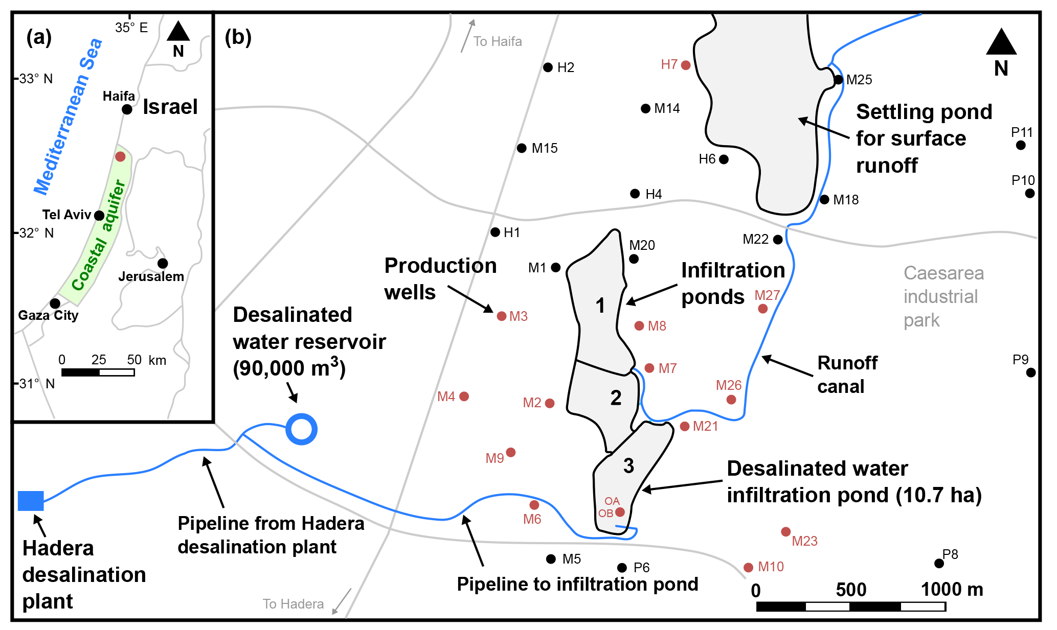
Figure 1Map of the study area. (a) Location of the Israeli coastal aquifer and the Menashe MAR site (red circle). (b) The Menashe MAR site. A surplus of desalinated seawater is delivered from the Hadera SWRO desalination plant (lower left) to the southern infiltration basin (pond 3). The red dots represent wells that were sampled for water isotope analysis.

Download

2.3 Groundwater flow and transport model

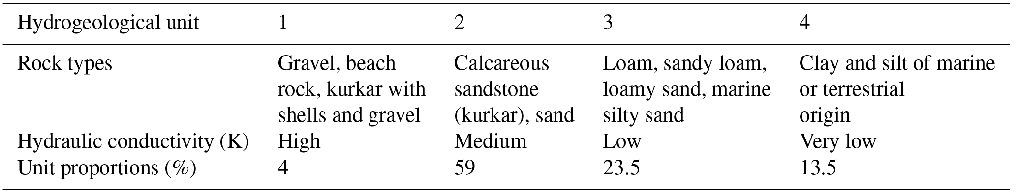
A detailed three-dimensional transient water flow and solute transport model was set up in order to estimate DSW spreading in the aquifer at the Menashe site area. The model covers an area of 65 km², including a western offshore strip of 9 km² (Fig. 2a). The geological data processed from well logs, geological maps and structural maps served as the basis for the conceptual model, constructed via the GMS software package (version 10.3; https://www.aquaveo.com, last access: 22 November 2018). The variety of rock types was grouped into four hydrogeological units, each characterized by a set of hydrological properties (Table 1). Over 100 well logs were analyzed using the T-PROGS software (Carle, 1999) and provided the spatial distribution of the hydrogeological units. This geostatistically generated unit array, conditioned to the borehole logs, was combined with structural map data of the major marine clay lenses present in the aquifer. The resulting model hence reflects the hydrogeological units' proportions and transition trends as well as the division into sub-aquifers by marine clay within the western part of the aquifer (Fig. 2b, c).

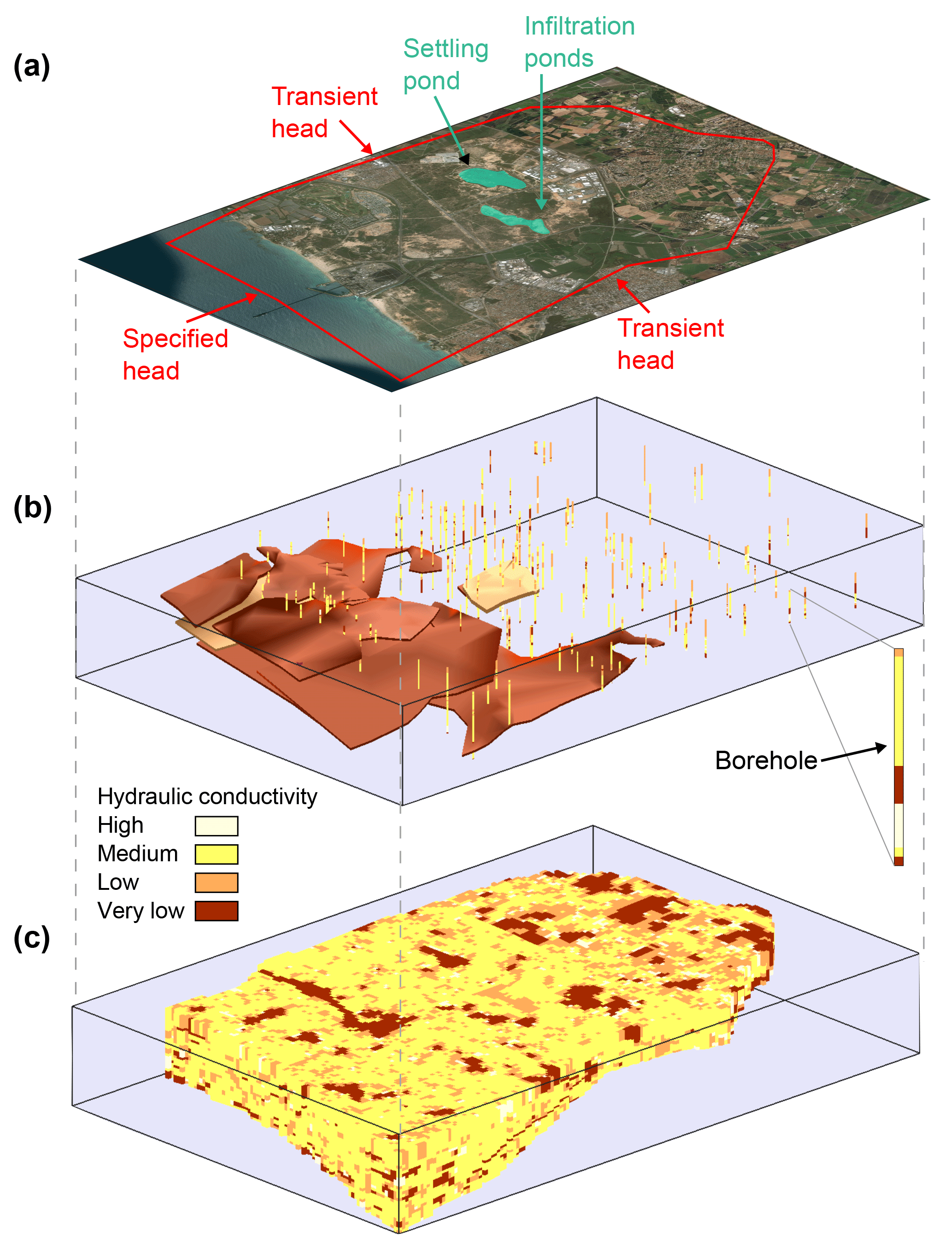
Figure 2The model used in simulations of water flow and solute transport. (a) The modeled area and boundary conditions. (b) The major continuous marine clay lenses and the borehole log. (c) The combined deterministic and geostatistically generated material array representing the aquifer in the model.

Download

Table 1Major rock types in the study area grouped into four hydrogeological units.

Download Print Version | Download XLSX

The model domain was discretized horizontally into 70×70 m mesh cells. The vertical section of the aquifer, with thickness ranging 50–100 m from east to west, was divided into 24 layers with a vertical spatial resolution of 5 m or smaller. The model's bottom boundary was defined by the impermeable Saqiye Group underlying the aquifer. The model's top boundary was defined by the water table representing an unconfined aquifer. Boundary conditions along the northern, eastern and southern model boundaries were set to be of a transient head type, based on periodic water level measurements. The western boundary was set to a constant head boundary dictated by the sea level. Initial conditions were based on static heads measured at several dozens of production and observation wells included in the model. Sources and sinks in the flow model include recharge by precipitation, MAR (both runoff and DSW recharge) and production wells. Natural recharge from precipitation was based on adjacent rain gauge measurements (Gan Shmuel), using an average recharge coefficient of 0.4 (which is representative of sands). Recharge flux of DSW by MAR activity was calculated by a variably saturated model of the upper 30 m of the sediment under the southern infiltration pond (Ganot et al., 2017). Pumping activity of the production wells was based on a database from the national water company of Israel, Mekorot.

The transport model considers the stable water isotopes ¹⁸O and ²H as conservative tracers, i.e., neglecting isotope fractionation (there is strong evidence that local groundwater tends to be isotopically uniform, see for example Krabbenhoft et al., 1990 and references therein). We normalize the tracer concentration as $C=(\mathit{\delta }-{\mathit{\delta }}_{\min })/({\mathit{\delta }}_{\max }-{\mathit{\delta }}_{\min })$, where δ is the isotope composition of δ¹⁸O or δ²H in the aquifer, and δ_min and δ_max are the minimum and maximum isotope composition, respectively. Since practically δ_max=δ_DSW, the normalized concentration of DSW is C_DSW=1, whereas that of GW ranges from C_GW=0 (δ¹⁸O = −5.43 ‰, δ²H = −22.68 ‰) to C_GW=0.13 (δ¹⁸O = −4.48 ‰, δ²H = −18.41 ‰). Boundary conditions of the transport model are of specified mass flux (qC, where q is the specific discharge), with zero flux at the bottom boundary (considered impermeable) as well as zero flux at the northern, eastern and southern boundaries, and also with the precipitation and the runoff-pond source terms, due to their GW isotope compositions (C_GW=0). Mass flux with the DSW isotope composition (C_DSW=1) is given at the western boundary (sea) and the DSW infiltration pond source term. The validity of the use of a single value (C_GW=0) for the GW mass-flux boundaries, in light of the range of isotope compositions in the aquifer prior to the MAR of DSW (δ¹⁸O = −4.48 ‰ to −5.43 ‰ and δ²H = −18.41 ‰ to −22.68 ‰), is discussed in Sect. 3.2.3. Initial conditions were set by interpolating the water isotope data from several production wells.

The MODFLOW (Harbaugh et al., 2000) and MT3DMS (Zheng and Wang, 1999) codes were used through the GMS user interface to numerically solve the flow and transport models, respectively. Both codes, which use a finite difference scheme, are considered reliable and are therefore widely used for regional aquifer modeling (Zhou and Li, 2011). The flow and transport model was calibrated using a dataset from 2015 to 2017. During 2015, 2016 and 2017 a volume of 2.6, 1.3 and 0.6 MCM of DSW were recharged, respectively, at the Menashe MAR site. In these years the MAR events consisted of a noncontinuous discharge of DSW to pond 3 (Fig. 1b) during January and/or February (Ganot et al., 2017, 2018). In addition, a volume of 3.2 and 1.6 MCM of runoff water were discharged to the settling pond during 2015 and 2017, respectively.

3.1 Water isotopes

The distinct difference between the water isotopes of the production wells and DSW is shown in a δ²H vs. δ¹⁸O diagram for the period of 2015 to 2017 (Fig. 3a and Table S1 in the Supplement). During 2016, and more prominently in 2017, few wells showed a progressive change in composition towards higher isotope values – a transition from GW towards DSW on the mixing line (Fig. 3a) indicates mixing with DSW – while most wells retain a constant isotope composition. Note that for all samples in Fig. 3a, there is a strong linear correlation between δ¹⁸O and δ²H (R²=0.9991); thus, hereafter we only report δ²H as a tracer.

Figure 3(a) Water isotopic composition of the production wells (GW) and reverse-osmosis desalinated seawater (DSW); the eastern Mediterranean meteoric water line (EMMWL) is shown for comparison (Gat and Dansgaard, 1972). (b) Chloride (Cl⁻) and δ²H sampled in nine production wells at the Menashe MAR site.

Download

The isotope composition of δ²H and the concentration of chloride are shown for comparison in nine wells during the years 2010 to 2018 (Fig. 3b). The chloride concentration of DSW at the Menashe MAR site is always lower than 10 mg L⁻¹ (Ganot et al., 2018), while in the local GW it is found in a wider range of 40 to 140 mg L⁻¹. The large chloride concentration variability in the different wells prior to MAR with DSW (before 2015) suggests that various water sources feed the aquifer (as there is no extensive soluble salt layer in the aquifer according to the recent available geological data). Moreover, the breakthrough of DSW in wells M2, M6 and M9, captured by an increase in δ²H, is not reflected in the chloride concentration (expected to decrease). This implies that chloride – in general a widely used conservative tracer – is less sensitive to reverse-osmosis DSW in natural, fresh GW systems and therefore less useful for its detection.

Finally, we note that the very different DSW signature, in terms of δ²H from the other water sources in the Menashe site, reduces the problem of mixing various water sources to a binary system: (i) DSW and (ii) all other natural sources. This is because the signatures of runoff water (δ¹⁸O = −4.77 ‰ and δ²H = −19.5 ‰) and rainwater (δ¹⁸O = −5.8 ‰ and δ²H = −19.9 ‰; Gat and Dansgaard, 1972; Goldsmith et al., 2017) are very similar to that of the local GW. Therefore, the binary system approach used in this study, which is based on conservative water isotope tracers is superior to both conservative and nonconservative chemical tracers.

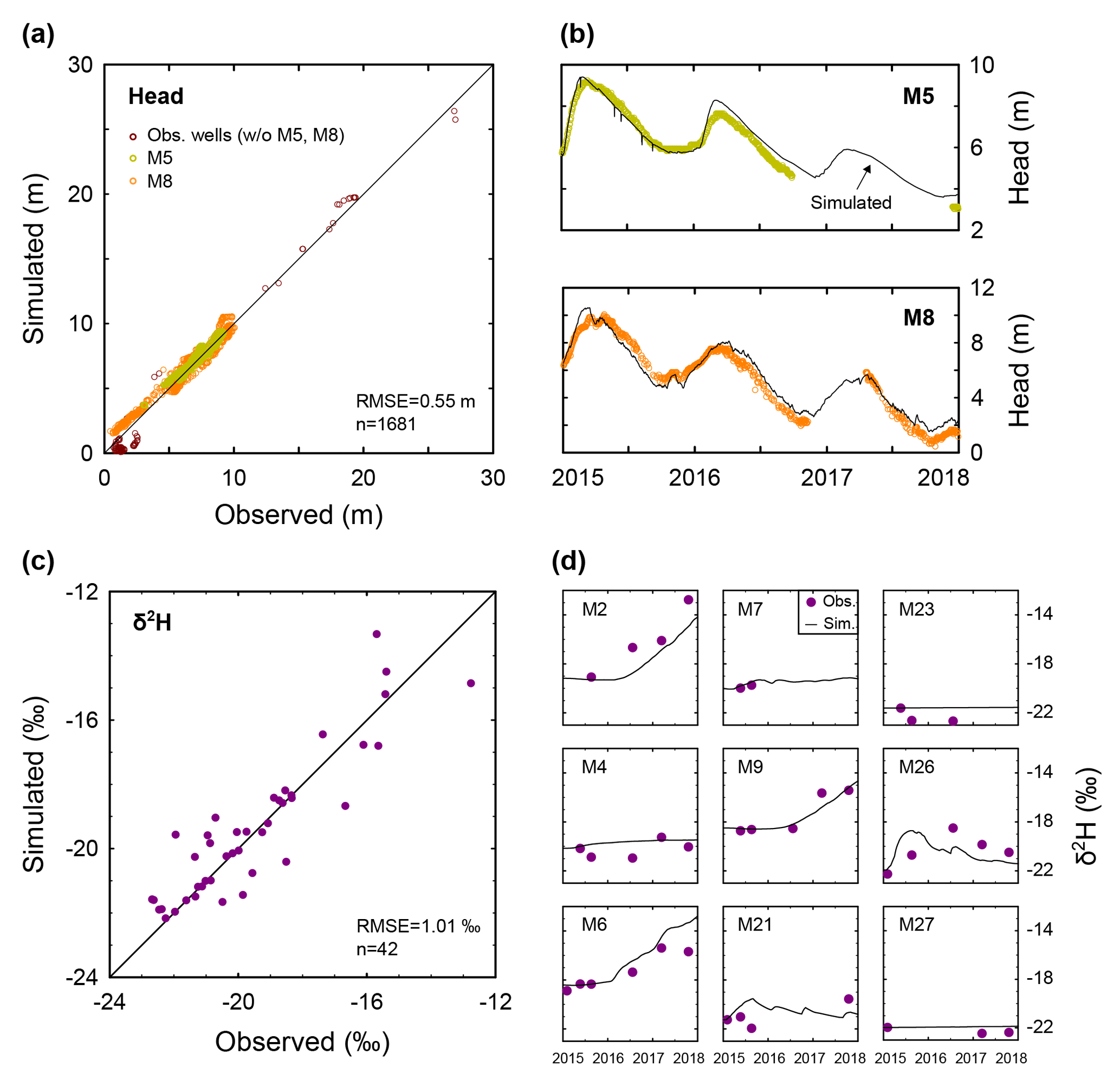
Figure 4Model calibration. (a) Comparison of the simulated and observed hydraulic head. (b) Temporal variations of the simulated and observed hydraulic head in wells M5 and M8. (c) Comparison of the simulated and observed δ²H. (d) Temporal variations of the simulated and observed δ²H in nine selected wells.

Download

3.2 Model

3.2.1 Calibration

The flow model was calibrated against head data from 13 wells (Fig. 4a). We mainly used continuous head data measured at two production wells, M5 and M8 (Fig. 4b). Well M5, situated 400 m SE of pond 3, exploiting aquifer layers bounded between −16 and −54 m MSL, was inactive during 2015–2017, making it ideal for head monitoring. Well M8, situated 1 km north of pond 3, exploiting aquifer layers bounded between −14 and −48 m MSL, was used for production during some of the study period, and thus only selected head data (representing quasi-static heads) were used for calibration.

The transport model was calibrated against isotope data from 12 wells (M2–4, M6–10, M21, M23 and M26–27; Fig. 4c). Specifically, we used data corresponding to the breakthrough of DSW in the down-gradient (western) production wells near the DSW infiltration pond (M2, M6, and M9) since other wells showed smaller δ²H variations (Fig. 4d). The simulated groundwater heads and δ²H for the calibration period are generally in good agreement with the observations. The calibrated hydrological parameters are specified in Table 2.

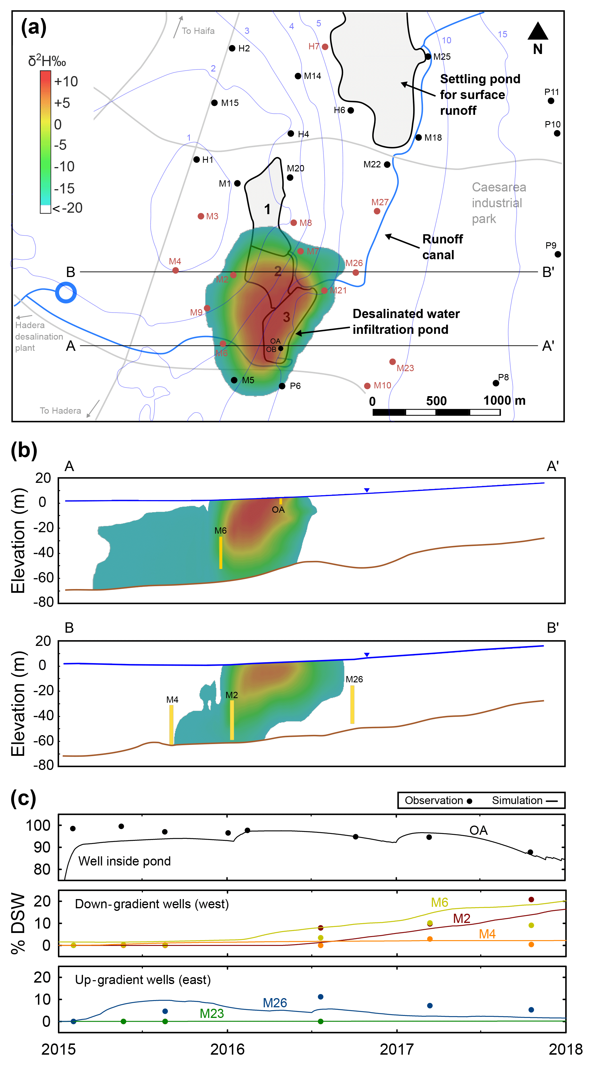
Figure 5Simulation results showing DSW spreading at the end of 2017. (a) Plan view (water table); the colored area shows the DSW plume, the white area indicates natural GW (δ²H < −20 ‰) and the blue contours are the GW head. (b) East–west cross sections through wells OA and M6 (A-A^′) and wells M4, M2 and M26 (B-B^′); well screens are shown in yellow. (c) Observed and simulated DSW fraction (%) in selected wells along the cross sections A-A^′ and B-B^′.

Download

Table 2Calibrated parameters used for the different hydrogeological units.

^* Transverse horizontal and vertical dispersivities are 0.1 and 0.01, respectively,
of the longitudinal dispersivity (Burnett and Frind, 1987).

Download Print Version | Download XLSX

3.2.2 DSW spreading in the aquifer

Our simulations show that at the end of 2017 the DSW plume was spreading westwards (in the direction of the natural hydraulic gradient, as expected), approaching the closest western production wells (M2, M6, M9; Fig. 5a). Note that the production wells to the east (up-gradient) show a constant δ²H, indicating no interaction with the DSW recharge. Variability of δ²H along the production well screens (in the vertical direction), implies that the measured δ²H is a mixture of several aquifer layers (Fig. 5b).

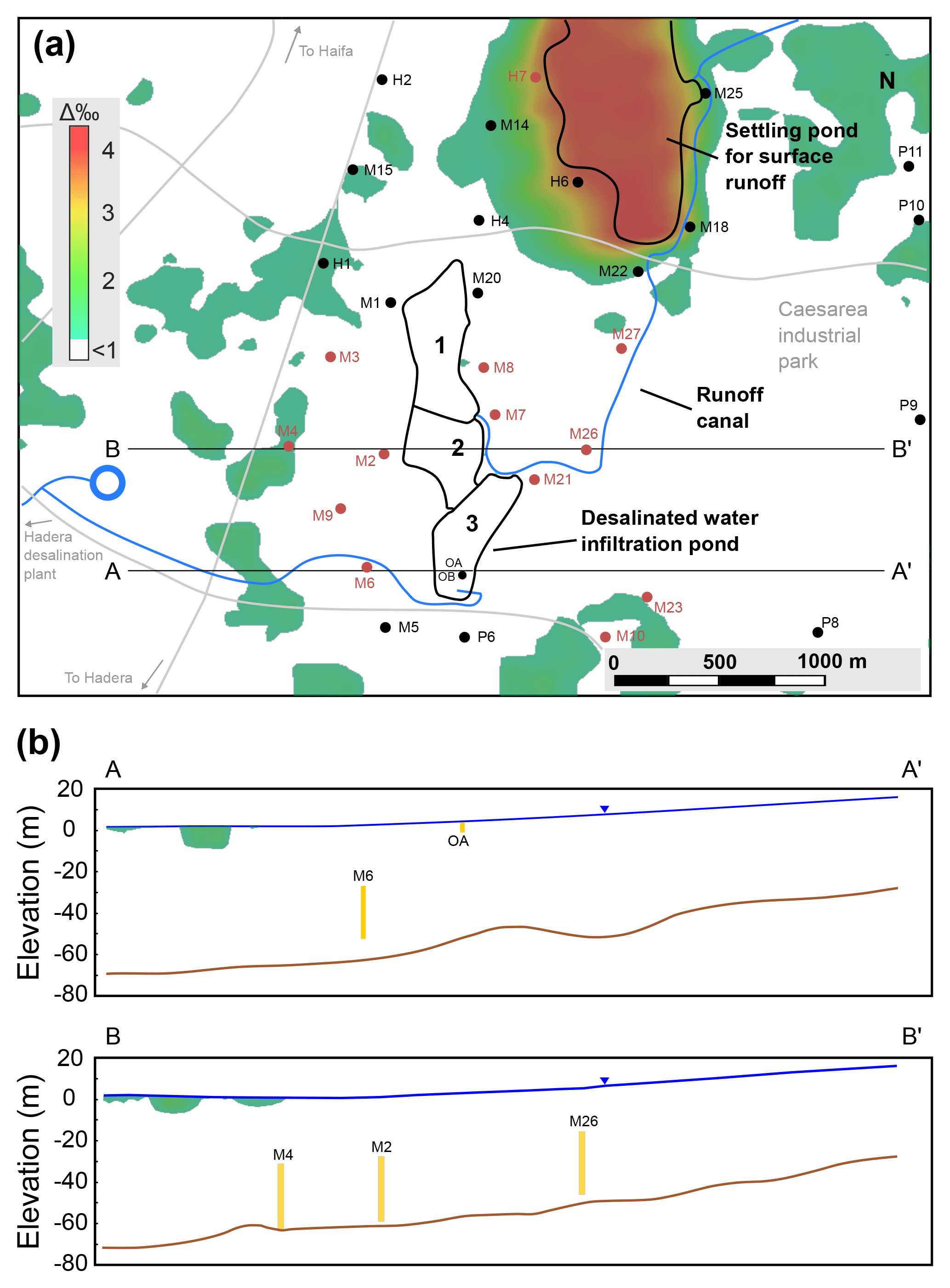
Figure 6Examination of the validity of the assumption of binary isotopic mixing. (a) Plan view (water table) of δ²H difference (Δ‰) between simulation results (2015–2017) with δ²H_max= −18.41 ‰ (C_GW=0.13) and δ²H_min= −22.68 ‰ (C_GW=0) at the end of 2017; the white area indicates Δ‰ < 1. (b) East–west cross sections through wells OA and M6 (A-A^′) and wells M4, M2 and M26 (B-B^′); well screens are shown in yellow.

Download

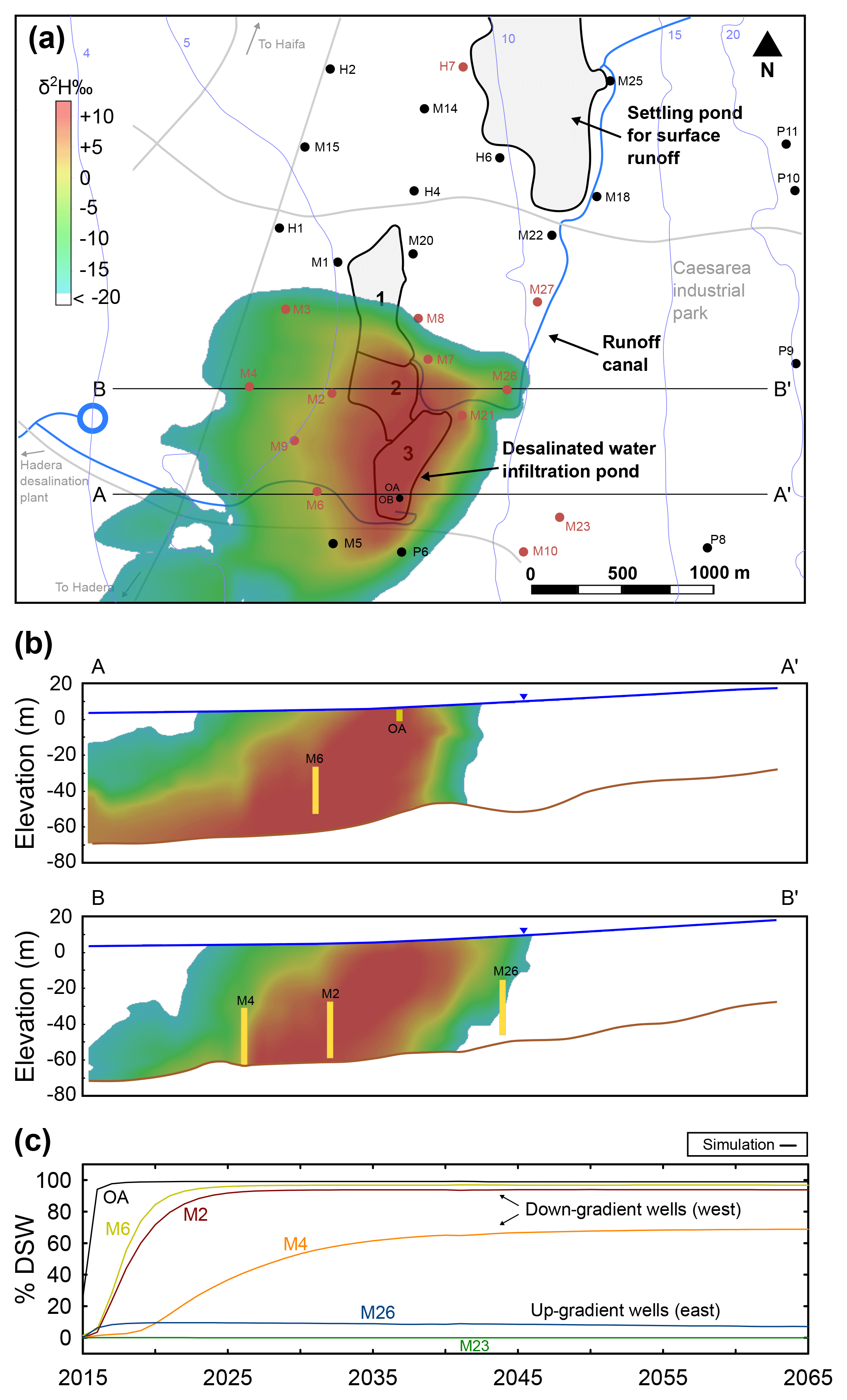
Figure 7Long-term simulations of DSW spreading at the end of 2065 after 50 years of MAR. (a) Plan view (water table); the colored area shows the DSW plume, the white area indicates natural GW (δ²H < −20 ‰) and the blue contours are the GW head. (b) East–west cross sections through wells OA and M6 (A-A^′) and wells M4, M2 and M26 (B-B^′); well screens are shown in yellow. (c) Simulated DSW fraction (%) in selected wells along the cross sections A-A^′ and B-B^′.

Download

The δ²H variations shown in Fig. 5a reflect the DSW spreading in the aquifer. The highest δ²H that was measured in the aquifer (prior to MAR of DSW) was δ²H = 18.41 ‰, and therefore any value above it indicates mixing with DSW. However, because the initial measured δ²H values in the aquifer are in the range of δ²H = −18.41 ‰ to −22.68 ‰, the extent of DSW mixing in each well is relative to its specific initial δ²H. This can be calculated by a mixing ratio (MR) approach with MR $=({\mathit{\delta }}_{\mathrm{w}}-{\mathit{\delta }}_{\mathrm{i}})$ ∕ (δ_DSW−δ_i), where δ_w is the δ²H in the well, δ_i is the initial (background) δ²H in the well and δ_DSW is the δ²H of DSW. The MR value of 0 and 1 implies original aquifer water and pure DSW, respectively. Figure 5c shows the MR (expressed in %DSW) of three down-gradient wells (M2, M4 and M6), two up-gradient wells (M23 and M26) and an observation well (OA) inside the DSW pond. Wells M2 and M6 have up to a 20 % DSW portion, while M23 and OA retain original aquifer water and almost pure DSW, respectively. At the end of 2017, about 7 % of the recharged DSW was recovered by the production wells.

Knowing the water composition of the aquifer and DSW, and assuming a conservative transport of all the major ions, one can estimate the water composition in a specific well based on the calculated mixing ratio, [X]_w= MR × $[X{]}_{\mathrm{DSW}}+(\mathrm{1}-\mathrm{MR})$ × [X]_i. Here [X]_w is the (calculated) ion concentration in the well, [X]_DSW is the ion concentration in the DSW and [X]_i is the initial ion concentration (background) in the well. Diversion of the observed concentration from the calculated concentration can give insight to the sediment–water reaction (e.g., Ganot et al., 2018; Ronen-Eliraz et al., 2017; Stuyfzand et al., 2017).