the Creative Commons Attribution 4.0 License.
the Creative Commons Attribution 4.0 License.
 | 10 Dec 2018
Using paleoclimate reconstructions to analyse hydrological epochs associated with Pacific decadal variability
George Kuczera
Anthony S. Kiem
Garry Willgoose
The duration of dry or wet hydrological epochs (run lengths) associated with positive or negative Inter-decadal Pacific Oscillation (IPO) or Pacific Decadal Oscillation (PDO) phases, termed Pacific decadal variability (PDV), is an essential statistical property for understanding, assessing and managing hydroclimatic risk. Numerous IPO and PDO paleoclimate reconstructions provide a valuable opportunity to study the statistical signatures of PDV, including run lengths. However, disparities exist between these reconstructions, making it problematic to determine which reconstruction(s) to use to investigate pre-instrumental PDV and run length. Variability and persistence on centennial scales are also present in some millennium-long reconstructions, making consistent run length extraction difficult. Thus, a robust method to extract meaningful and consistent run lengths from multiple reconstructions is required. In this study, a dynamic threshold framework to account for centennial trends in PDV reconstructions is proposed. The dynamic threshold framework is shown to extract meaningful run length information from multiple reconstructions. Two hydrologically important aspects of the statistical signatures associated with the PDV are explored: (i) whether persistence (i.e. run lengths) during positive epochs is different to persistence during negative epochs and (ii) whether the reconstructed run lengths have been stationary during the past millennium. Results suggest that there is no significant difference between run lengths in positive and negative phases of PDV and that it is more likely than not that the PDV run length has been non-stationary in the past millennium. This raises concerns about whether variability seen in the instrumental record (the last ∼100 years), or even in the shorter 300–400-year paleoclimate reconstructions, is representative of the full range of variability.


A pattern of Pacific ocean–atmosphere climate variability at decadal timescales has been identified and explored at various locations around the world, including Africa (Reason and Rouault, 2002; Hoell and Funk, 2014), eastern and southern Asia (Krishnan and Sugi, 2003; Ma, 2007), America (Mantua and Hare, 2002; Andreoli and Kayano, 2005), and Australia (Kiem et al., 2003; Verdon et al., 2004; Verdon and Franks, 2006; Henley et al., 2011). This pattern, referred to in this paper as Pacific decadal variability (PDV), is associated with sea surface temperature fluctuations and sea level pressure changes in the North and South Pacific Ocean.
PDV is usually described by the Inter-decadal Pacific Oscillation (IPO) or Pacific Decadal Oscillation (PDO) indices (Mantua et al., 1997; Power et al., 1999). Of particular hydrological relevance are the statistical characteristics of PDV phases where a phase refers to a period during which the PDV index lies above (or below) some thresholds (Dong and Dai, 2015; Verdon et al., 2004; Henley et al., 2011; Vance et al., 2015). The duration of a PDV phase (termed run length) is defined as the time between consecutive crossings of the threshold. The phase may be described as positive (negative) if the PDV index is above (below) the threshold, or dry (wet) if the PDV phases are associated with predominantly dry (wet) hydrological conditions.
Of particular relevance to the hydrology and water resources community is the evidence that the PDV phases can be associated with multi-decadal periods of persistently wetter or drier conditions and corresponding increases in flood or drought risk in affected regions, particularly those on the Pacific rim. PDV has been found to be related to a number of hydrological variables including precipitation, streamflow, and flood and drought risk (Cook et al., 2013; Kiem et al., 2003; Verdon et al., 2004; Dai, 2013; Goodrich and Walker, 2011; Hu and Huang, 2009; Li et al., 2012; McCabe et al., 2012; Mehta et al., 2011; Wang et al., 2014; Henley et al., 2013). For example, Kiem and Franks (2004) showed in a case study for eastern Australia that the probability of reservoir storages falling below a critical level differs significantly depending on the PDV phases (see Fig. 6 in Kiem and Franks, 2004). Kiem and Franks (2003) and Micevski et al. (2006) demonstrated that flood risk in eastern Australia is strongly dependent on PDV phase. Henley et al. (2013) extended this work to show that short-term drought risk is strongly dependent not only on the PDV phase but also on the time spent in a particular phase.
Despite the clear relevance of PDV phases to hydrological risk assessment and water resource management, there remain considerable knowledge gaps about the statistical characteristics of PDV, including run lengths. The instrumental record shows that PDV phases have varied irregularly, with runs ranging from less than a decade to several decades during the past century. However, the instrumental record is insufficient to characterize the statistical characteristics of PDV run lengths. In response to this, significant advances have been made in reconstructing pre-instrumental PDV behaviour to extend data length. For example, at least 12 IPO or PDO reconstructions have been published (Biondi et al., 2001; Gedalof and Smith, 2001; D'Arrigo et al., 2001; MacDonald and Case, 2005; D'Arrigo and Wilson, 2006; Shen et al., 2006; Verdon and Franks, 2006; Linsley et al., 2008; Mann et al., 2009; McGregor et al., 2010; Henley et al., 2011; Vance et al., 2015).
In view of these published PDV reconstructions, the fundamental question is whether useful information can be extracted about the statistical characteristics of PDV persistence. In dissecting this question, several unresolved issues are identified:
-
Static threshold methods have been used to estimate run lengths of PDV phases. This raises the concern that biased conclusions about the statistical characteristics of decadal climate variability may be drawn when reconstructions exhibit centennial or longer trends. The non-parametric Mann–Whitney test method was used in Verdon and Franks (2006) whereby a crossing was defined when the test detected a statistically significant difference between two halves of data in a 30-year moving window, with zero used as a static threshold to define the sign of PDV phases (Danielle C. Verdon-Kidd, personal communication, 24 April 2017). Henley et al. (2011) used the instrumental mean of the composite IPO–PDO index. After standardizing the indices, Vance et al. (2015) used ±0.5 as thresholds to determine crossings and the sign of PDV phases, and Henley et al. (2017) used the long-term modelled IPO tripole index (TPI) mean as the static threshold with run lengths less than 5 years omitted. However, when static threshold methods are used, extraordinary long centennial run lengths may be identified in the reconstructions that exhibit centennial or longer trends (MacDonald and Case, 2005; Mann et al., 2009). Analysis based on data with long-term trends can lead to results that are overwhelmed by such trends and hence efforts have been made to detrend data without losing useful signals (Wahl et al., 2006; von Storch et al., 2006; Wu et al., 2007). As stated by von Storch et al. (2006), “it is commonly accepted that proxy indicators may contain non-climatic trends”. Moreover, the calibration and validation of any statistical method using non-detrended data may be compromised because the non-climatic trends may be interpreted as a climate signal. The centennial trends in PDV reconstructions may be either non-climatic trends or non-decadal climate trends. Whichever the case, it is necessary to filter such centennial trends before interpreting decadal climate variability. Given that static threshold methods cannot remove trends, how should the run length extraction method be designed to extract useful and consistent information from all reconstructions, including reconstructions exhibiting centennial trends? To what extent are run length distributions sensitive to the choice of extraction parameters (e.g. threshold, window width)?
-
The durations of positive and negative PDV phases have not been treated separately in most previous research (e.g. Verdon and Franks, 2006; Linsley et al., 2008; Henley et al., 2011a). Using a high-resolution millennial-length IPO reconstruction, Vance et al. (2015) observed that positive phases dominate and last longer than negative phases. Owing to non-linear hydrologic feedback mechanisms, such as elasticity of streamflow to runoff (Chiew, 2006) and shifted rainfall–runoff relationships (Saft et al., 2015), the duration of increased (decreased) precipitation during a wet (or dry) PDV phase may impact on streamflow in a highly non-linear manner. Therefore, assuming wet and dry runs follow the same distribution may misrepresent the intensity of impacts. Is there sufficient evidence about the dissymmetry between positive and negative phase run lengths from the multiple reconstructions? Will run length samples from each phase lead to significantly different run length simulations?
-
Stationarity of climate signatures is a necessary, yet implicit, assumption underlying many analyses based on paleoclimate reconstructions – and hydroclimate stochastic modelling used in water resource assessment (e.g. Henley et al., 2013). However, a number of studies have suggested the possibility of climatic non-stationarity over the past millennium. Phipps et al. (2013) found that the relationships between paleoclimate proxies and climatic variables have been changing at least throughout the last millennium. Razavi et al. (2015) explored the stationarity of the mean, variance and autocorrelation structures of paleo-tree-ring proxy data and concluded that the key statistical characteristics of climate had undergone significant change over time. The existence of extraordinary warm and cold periods, known as the Medieval Climate Anomaly (∼950–1250 CE) and Little Ice Age (∼1400–1700 CE) (Mann et al., 2009; Phipps et al., 2013; Atwood et al., 2015), also challenges the assumption of climatic stationarity. Furthermore, externally forced anthropogenic climate change, arising from elevated atmospheric concentrations of greenhouse gases, may also make recent and future climate different from the distant past (Kirtman et al., 2013). Therefore, care should be taken when positing that PDV characteristics are stationary. Statistical signatures of past reconstructed PDV runs should be tested for non-stationarity (and where possible non-stationarity should be attributed to causal mechanisms) to ensure robust and representative estimation of the full range of variability.
In view of the above-mentioned issues, this study has the following objectives:
-
To develop a more robust run length extraction method that is applicable to all reconstructions, including those with centennial trends. Of particular importance is the sensitivity of the inferred run length distributions to the choice of the extraction method parameters.
-
To identify hydrologically important statistical properties of PDV that are common to different reconstructions. In particular two fundamental questions are explored: (i) whether persistence (i.e. run lengths) during positive epochs is different to persistence during negative epochs and (ii) whether the reconstructed run lengths have been stationary during the past millennium. Both questions address fundamental concerns about using PDV and run length information in stochastic hydroclimatic models used to assess drought and flood risk.
The rest of the paper is organized as follows. Section 2 briefly introduces the instrumental and reconstructed PDV records used in this research. The dynamic threshold run length extraction method is introduced in Sect. 3, along with its comparison with the static threshold method and determination of its parameters. The hydrologically important statistical signatures of PDV are analysed and discussed in Sect. 4, with conclusions presented in Sect. 5.
2.1 Instrumental PDV records
A number of instrumental IPO and PDO indices have been published to characterize PDV since ∼1900. There is a strong correlation between IPO and PDO indices, suggesting that both indices represent a similar broad pattern of climate variability. The primary difference between the IPO and PDO indices is that the IPO index is based on a broader spatial scale than the PDO index (Folland et al., 2002; Verdon and Franks, 2006; Henley et al., 2011).
Three PDV indices are used in this study: (1) the unfiltered instrumental PDO index (http://research.jisao.washington.edu/pdo/PDO.latest.txt, last access: 22 September 2016), denoted as PDO_Mantua, is the monthly standardized value of the leading principal component of monthly sea surface temperature (SST) anomalies in the North Pacific Ocean, poleward of 20∘ N (Mantua et al., 1997; Zhang et al., 1997); (2) the unfiltered monthly IPO index from Parker et al. (2007), denoted as IPO_Parker, is the second covariance empirical orthogonal function of low-pass-filtered SST; (3) the unfiltered monthly tripole index for the IPO (Henley et al., 2015), denoted as IPO_Henley, is based on the SST anomalies in three large geographic regions of the Pacific. Annual (calendar year) values of these three indices are taken as the average of monthly values.
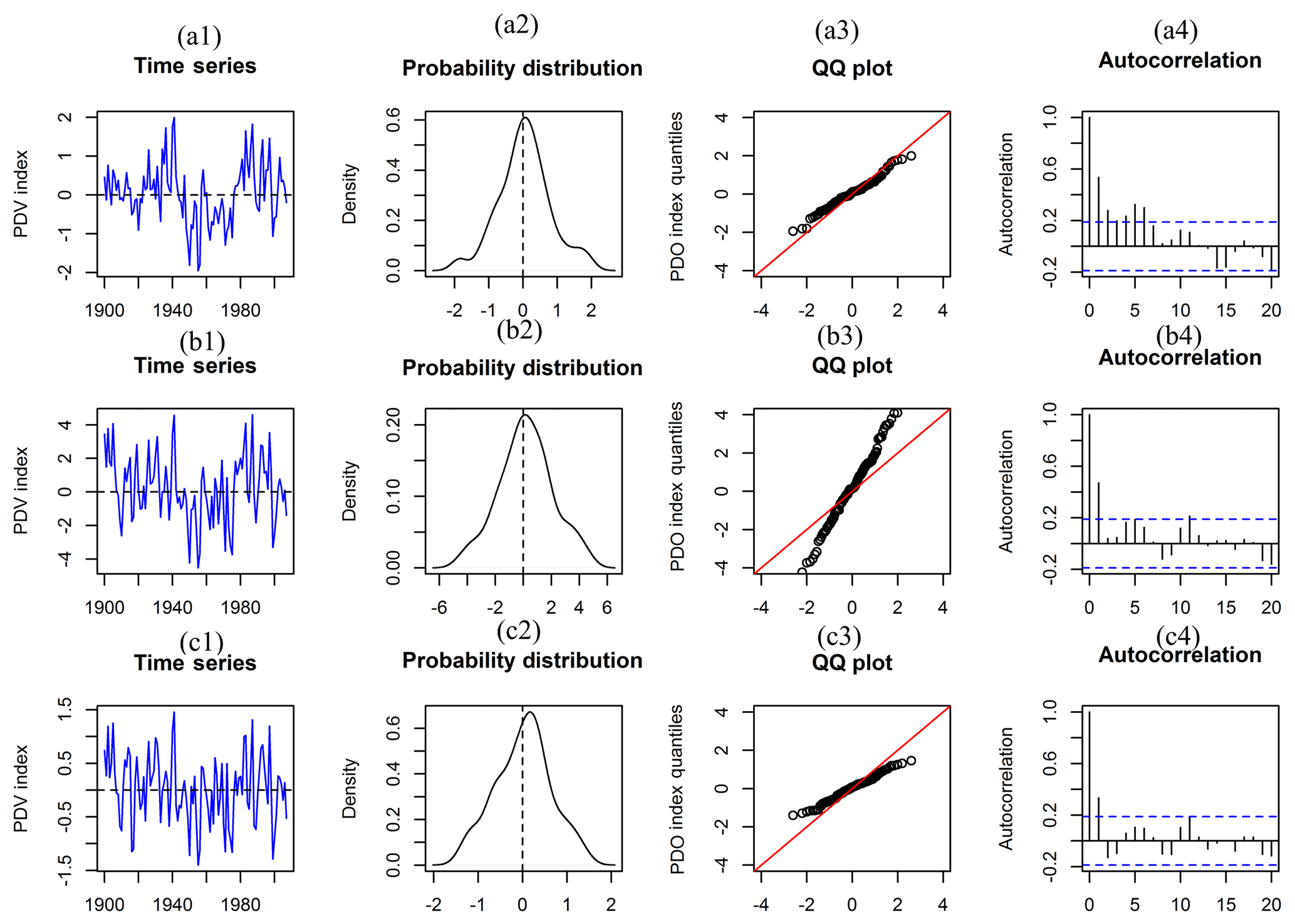
Figure 1Annual instrumental time series, probability density plot, QQ plot and autocorrelation plot: (a) PDO from Mantua (1900–2015); (b) IPO from Parker (1871–2007); (c) IPO from Henley (1870–2007).
Figure 1 shows time series of the three indices along with probability density plot, quantile–quantile (QQ) plot and autocorrelation plots. The distribution density plot and QQ plot of the annual PDV indices suggest that the instrumental PDV indices are approximately normally distributed with zero mean and unit standard deviation (except for IPO_ Parker). The lag-one autocorrelation lies between about 0.3 and 0.5. By lag three, the autocorrelations lie within the 95 % confidence bands for zero autocorrelation.
The instrumental PDV indices are used for two purposes in this study:
- a.
To assess the similarity between IPO and PDO indices. If instrumental IPO and PDO indices can be used to represent the same broad pattern of climate variability – and noting that different reconstructions are calibrated against different instrumental indices – there is no need to recalibrate all reconstructions against the same instrumental data.
- b.
To guide the selection of the parameters of the run length extraction method. If selected parameters can identify credible run lengths in the instrumental PDV record, it is assumed that they can also produce credible run lengths in the reconstructed record.
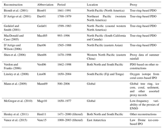
Table 1Available PDV paleoclimate reconstructions and their descriptions.
2.2 PDV reconstructions
A total of 12 published annual PDV reconstructions from different sites with different proxies are used in this study. Of these, nine reconstructed the last 300–400 years and three reconstructed the last ∼1000 years. The reconstructions are based on paleo-proxies (i.e. preserved physical characteristics of the environment that can be directly measured) from the northern, southern, western and eastern regions of the Pacific Ocean. A summary of these reconstructions is presented in Table 1, while Fig. 7 in Sect. 3.2.3 presents time series plots of the 12 reconstructed indices, and they are denoted throughout by the four-character author name and two-character publishing year. It is worth noting that Mann09 was not directly calibrated to an instrumental PDV index, and also has a negative correlation with other reconstructions. However, because the correlation of this reconstruction with the other ones is relatively high (Henley, 2017), the Mann09 reconstruction is retained with the sign reversed.
3.1 Static and dynamic threshold run length extraction methods
However, for reconstructions Macd05, Mann09 and Vanc15, which exhibit centennial trends (see Table 1 and Fig. 2), the above-mentioned static threshold methods used in Verdon and Franks (2006), Henley et al. (2011, 2017) and Vance et al. (2015) may not identify meaningful decadal phases. Extraordinary long run lengths are identified if the overall mean is used as a threshold, with some runs lasting several centuries (see Fig. 2). It is not clear whether these centennial trends are due to low-frequency climate variability or due to unknown local factors affecting the proxy. With such reconstructions, one can either exclude them from analysis or filter out the centennial trends. Exclusion forgoes any useful information from the reconstructions. On the other hand, filtering out the centennial trends offers the prospect of extracting possibly useful information about run lengths.
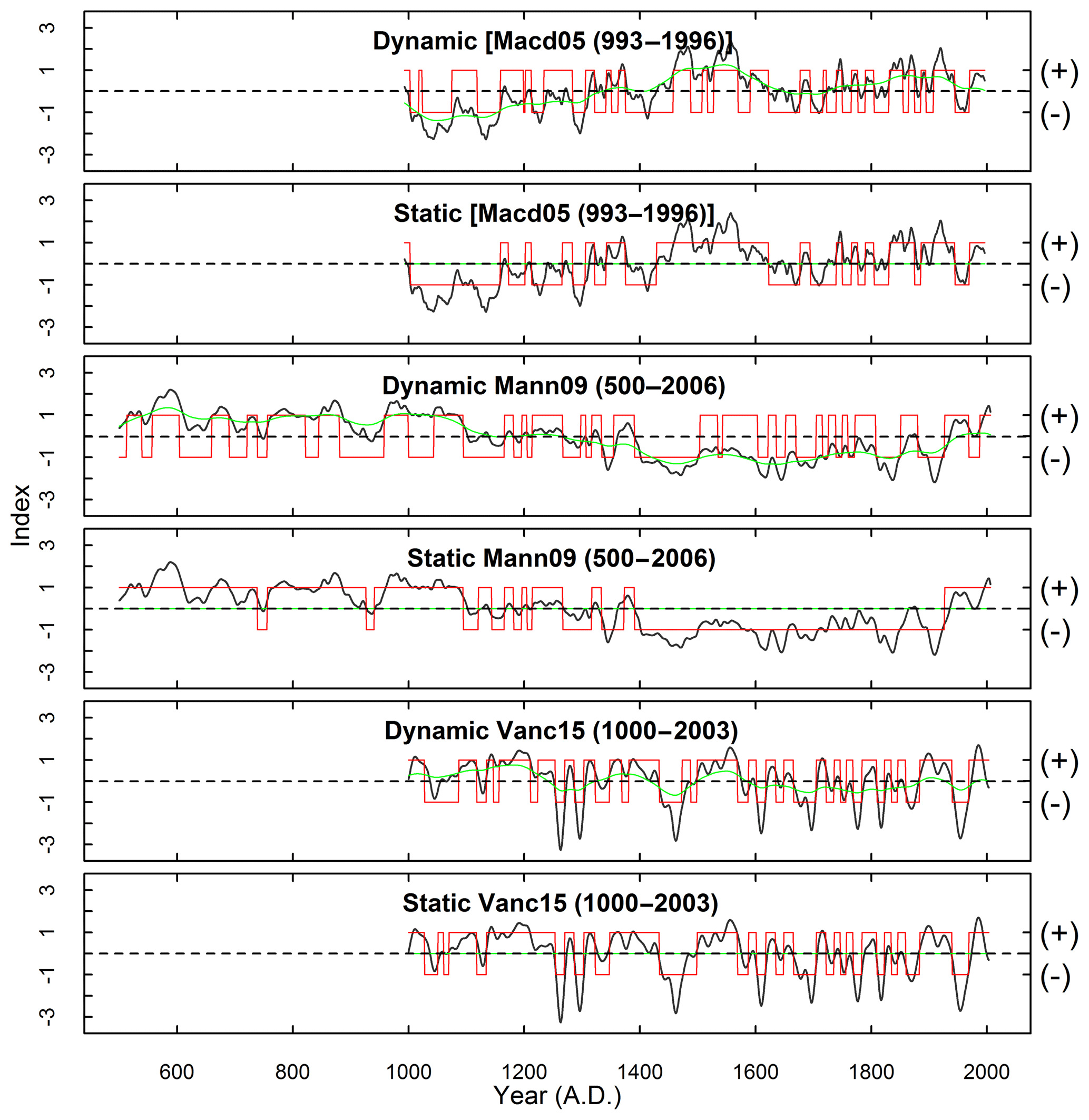
Figure 2Run length time series extracted using the dynamic and static threshold methods for reconstructions with centennial trends.
We adopt the latter approach, proposing a dynamic threshold framework to filter out centennial trends. In this framework, potential crossings are taken to be the change points detected by the Mann–Whitney test, and the sign of PDV phases is determined by a dynamic threshold that takes centennial trends into consideration – this relaxes the restriction of a static threshold defining a phase crossing. Figure 2 provides insight into the mechanics of dynamic threshold method, showing the PDV time series and the resulting block phase waveform. The key steps of this framework are as follows:
-
Detect step-change points. For a given reconstruction, apply a change point detection method. A number of methods can be used. In this study we used the non-parametric Mann–Whitney test method (Mauget, 2003) with a given window width w and confidence level α to identify the step-change points. The method involves centring a window of width w at a particular year t and then applying the Mann–Whitney test to the samples of width w∕2 at or before and after year t. A step change is deemed to occur if the Mann–Whitney test statistic lies outside the α confidence limits (under the null hypothesis).
-
Merge consecutive step-change points. When two or more step change points occur in consecutive years, replace them with a single change point. That is, if there are either 2n−1 or 2n years that are determined as consecutive change points ( …), replace them with one change point at year n. This guarantees that the new change point is always closest to the middle of the run of consecutive step-change points.
-
Assign a phase to each run defined by the interval bounded by two step-change points. Let i(t) denote the PDV index in year t, if(t) the filtered PDV index using a first-order Butterworth filter (which was used by Henley et al. (2011) to filter paleo PDV indices) with cut-off frequency 1∕ yr−1, the year that the kth change point occurs (from steps 1 and 2) and s(t) the phase state of year t. The mean PDV index for the kth run is
while the corresponding mean of the filtered index is
The phase of the kth run length is then defined by
Determine run lengths using the time series s(t). The run length of the kth run will be .
This dynamic threshold method can be seen as a generalization of previous run length extraction methods. If parameter y is set to the total number of years in a given reconstruction, the dynamic threshold method reduces to the method used in Verdon and Franks (2006). If change points are defined by the PDV index crossing the threshold and the cut-off frequency parameter y of the first-order Butterworth filter is set to the total number of years in the reconstruction, the dynamic threshold reduces to the method used in Henley et al. (2011, 2017).
Three parameters need to be specified in the dynamic threshold method: window width w and confidence level α in the Mann–Whitney test, and cut-off frequency y of the Butterworth filter. The standard cut-off frequency parameter in the dynamic threshold method is used to filter out centennial trends that may be mixed with decadal variability and should have little influence on the statistical characteristics of the inferred runs. A cut-off frequency of 1∕100 years is considered to adequately meet these requirements. Hence, y=100 is used in this study. In this study, we set the confidence level to be 90 %, a value that is consistent with other reconstruction studies (e.g. Gedalof and Smith, 2001; Shen et al., 2006; McGregor et al., 2010; Peng et al., 2015). It has been shown that reconstructions are sensitive to the choice of the window used in the Mann–Whitney test as well as the choice of threshold (Henley et al., 2017; Henley, 2013). Accordingly, this study investigates the sensitivity of dynamic threshold method results to the choice of window width w in the Mann–Whitney test. This sensitivity analysis is used to guide the selection of parameters to be used in the analysis of all 12 PDV reconstructions.
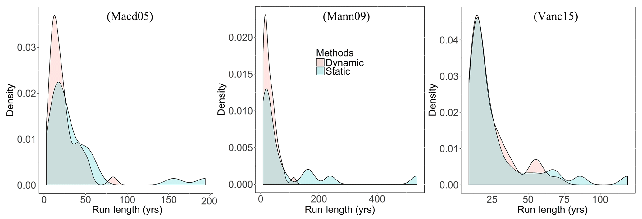
Figure 3Comparison of run length distributions extracted using the dynamic and static threshold methods in reconstructions with centennial trends.
3.2 Results from different run length extraction methods
3.2.1 Comparison of static and dynamic threshold
To further demonstrate the shortcomings of the static threshold method and the need for a dynamic threshold method, run length samples are extracted using the dynamic threshold method proposed in this study (denoted as “Dynamic” in the figures) and the static threshold method used in Verdon and Franks (2006) (denoted as “Static” in the figures). These two methods only differ in step 3 of Sect. 3.1. In the static method, the overall mean defined as (in which n is number of years in corresponding reconstruction) is used as the threshold instead of the dynamic threshold defined in Eq. (2). Extracted run length samples using the dynamic and static threshold methods from three millennium-long reconstructions with centennial trends are plotted in Fig. 2. Black lines are filtered standardized PDV indices; green lines represent the Butterworth (1∕100) filtered data in the dynamic plots and the overall mean in the static plots; red lines represent the run extracted using either the dynamic or static thresholds method. The run length distributions are plotted in Fig. 3.
It is shown in Fig. 2 that extraordinarily long runs are identified when the static threshold method is used – the stronger the centennial trends, the longer the runs. On the other hand, use of the dynamic threshold framework appears to filter centennial trends and produce more meaningful run lengths. The run length density plots show that the dynamic threshold method for the Macd05 and Mann09 reconstructions removes centennial-scale runs. In the case of Vanc15 the centennial trends are muted, possibly because Vanc15 is annually resolved and very accurately dated (Vance et al., 2015) and as such is more likely to exhibit more realistic annual to decadal variability than Macd05 and Mann09 (see also Fig. 2). Individual reconstructions are subject to different error structures and magnitudes. Use of multiple reconstructions can help reduce the impact of errors, and thus provide more insight into the statistical characteristics of PDV run lengths. Nonetheless, errors still need to be carefully considered. This is illustrated by Henley et al. (2011), who combine individual reconstructions according to their accuracy. However, the accuracies of the individual reconstructions are not high (Nash–Sutcliffe indices < 0.48) suggesting that even favouring the more accurate individual reconstructions will still result in a combined or overall reconstruction with large errors. Therefore, the focus of our research is to identify a signal (or signals) that is (are) common to all individual reconstructions.
3.2.2 Window width sensitivity analysis
Henley (2013) demonstrated that the mean run length is strongly dependent on the choice of window width in the Mann–Whitney method and concluded that a subjective choice of window width is likely to bias the resulting run length distributions. To explore the sensitivity of window width on run length distributions, run length box plots for all reconstructions are plotted in Fig. 4 for window widths from 10 to 60 years with step of 2, with positive and negative samples plotted together and separately.
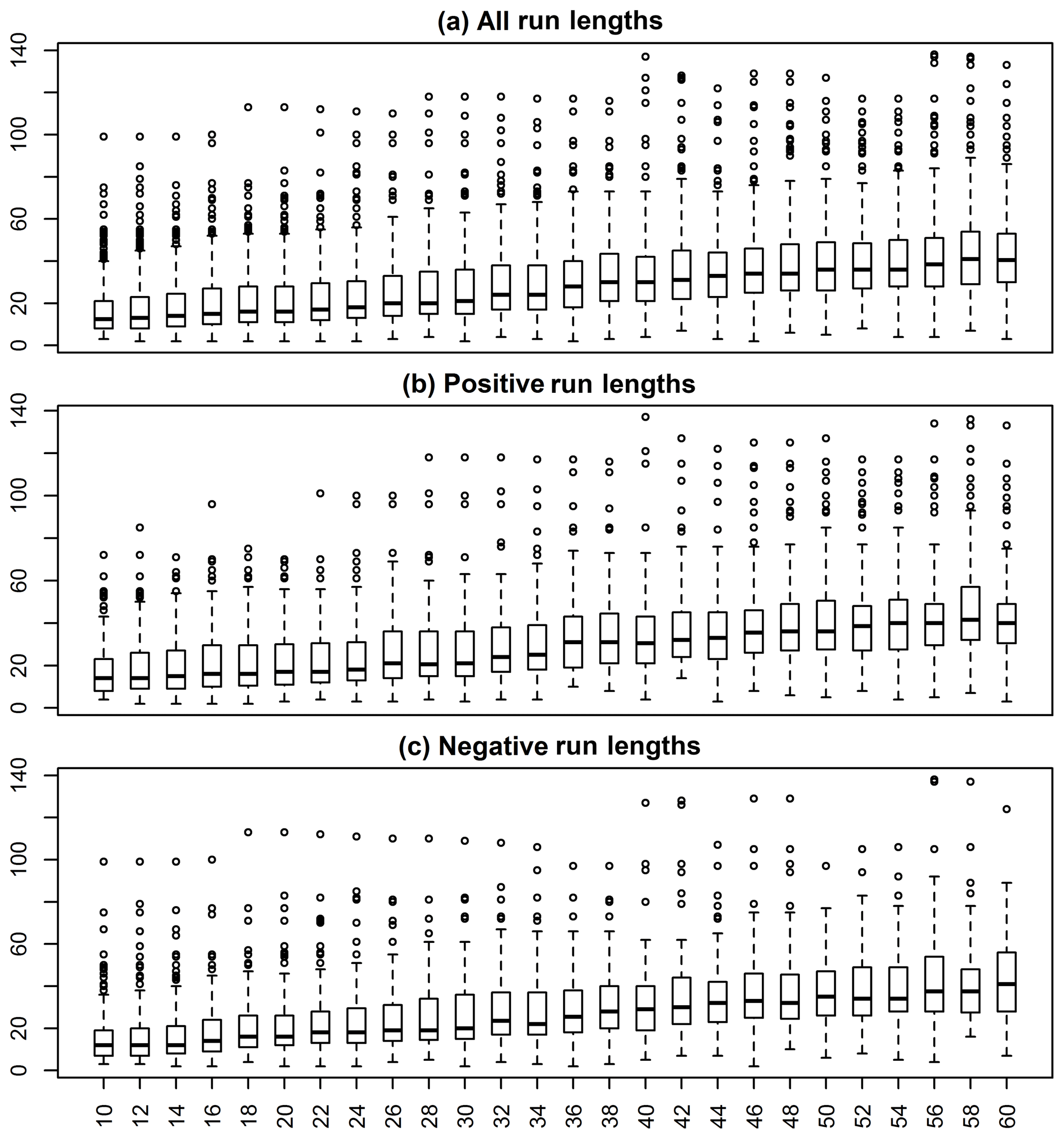
Figure 4Box plot of run length samples from all reconstructions with different window widths in the Mann–Whitney method.
Figure 4 shows that the run length distributions clearly depend on the choice of window width, with longer window widths leading to longer run length samples. However, the change is gradual, particularly for shorter window widths. As a result, run length distributions are not particularly sensitive to small variations in window width of the order of 10 years.
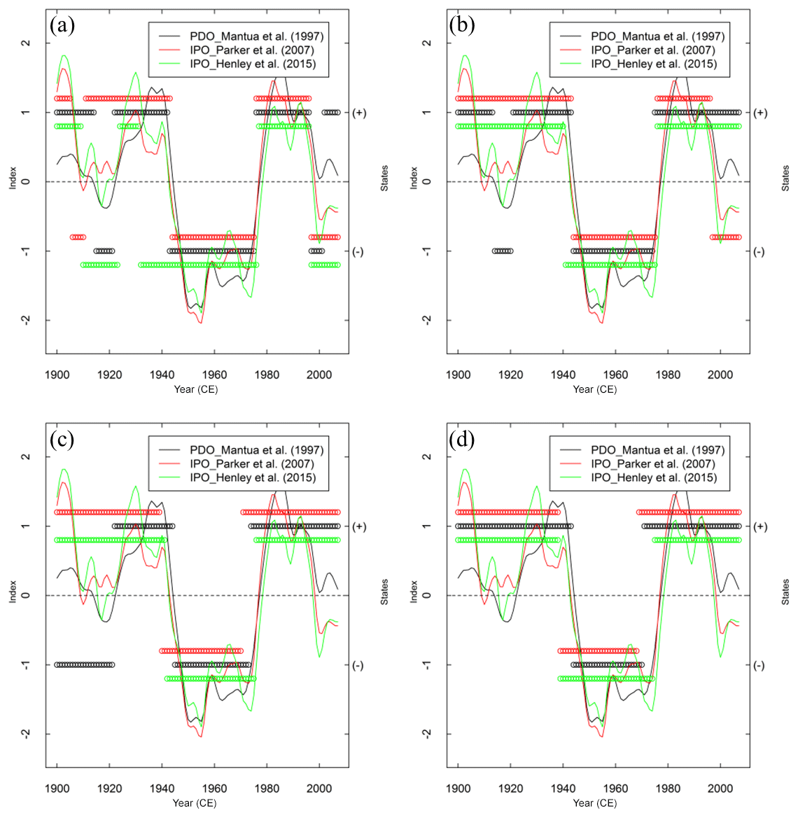
Figure 5Time series plots of different instrumental PDV indices and corresponding run lengths (represented by dots in corresponding colour) extracted using different windows: (a) 10, (b) 20, (c) 30, (d) 40 years.
3.2.3 Determination of parameters and application of dynamic threshold method
To guide the selection of an operationally useful window width, several window widths are applied to the three instrumental PDV time series to identify which produces results that match existing knowledge about run length in instrumental periods. Four window widths, 10, 20, 30 and 40 years, are applied to the instrumental time series with the extracted runs plotted in Fig. 5. Interpretation of Fig. 5 is illustrated for Fig. 5d. The green line represents the IPO_Henley index, from which three runs, denoted by green circles, are extracted: ∼1900–1938 (positive), ∼1938–1976 (negative), ∼1976–2004 (positive). These are very similar (in number, sign and duration) to the black (PDO_Mantua) and red run lengths (IPO_Parker). It can be seen that a window width of 10 years identifies very short runs which are more likely to represent random fluctuations rather than different PDV phases – we note that Henley et al. (2017) discarded runs with lengths less than 5 years. However, for the longer window widths of 20, 30 and 40 years, the differences become more muted.
To better understand these differences, consider window widths of 20 and 40 years. When the 40-year window is used, the first 20 years of the window are compared to the last 20 years. As a result, runs of less than 20 years may be overlooked. To demonstrate this, different window widths are applied to all reconstructions to extract run lengths, from which conditional run length distributions are determined. Figure 6 presents run length distributions in six panels. Panels (a1) to (a3) compare distributions for 20 and 40-year windows. Panel (a1) shows the empirical density of run lengths, while panels (a2) and (a3) show the empirical densities conditioned on run lengths less than 20 years and greater than 20 years respectively. Likewise panels (b1) to (b3) repeat this sequence for 20- and 60-year windows with the conditioning threshold of 30 years.
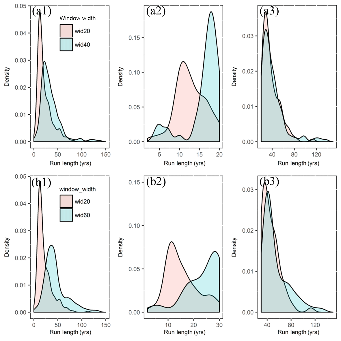
Figure 6Density plot of run length samples by applying different window widths to all reconstructions: (a1–a3) comparison between window width 20 and 40, in which (a1) is unconditional run length distribution, panel (a2) is the distribution conditioned on run lengths less than 20 years and panel (a3) is the distribution conditioned on run lengths greater than 20 years; (b1–b3) comparison between window width 20 and 60, in which (b1) is unconditional run length distribution, panel (b2) is the distribution conditioned on run lengths less than 30 years and panel (b3) is the distribution conditioned on run lengths greater than 30 years.
Panels (a1) and (b1) show that the unconditional run length distributions are different using different window widths with the difference greater for a greater difference in window width. However, panels (a3) and (b3) show that the conditional distributions for the longer runs are very similar. This shows that both the short and long window widths extract the longer runs in a largely consistent manner. However, the choice of window width strongly affects the distribution of shorter runs, as shown in panels (a2) and (b2). Overall, this demonstrates that shorter window widths can “see” higher frequency runs better than longer window widths but both “see” the same distribution of lower frequency runs.
These considerations suggest that the window width should be as small as possible, yet sufficiently big to filter out runs that are considered more likely to be random fluctuations rather than PDV phases. Therefore, in this study, a 20-year window is used to ensure decadal or longer runs are identified. Figure 7 plots the extracted runs for the 12 reconstructions using the dynamic threshold method with 90 % confidence limits and 20-year window in the Mann–Whitney test. The PDV indices plotted in Fig. 7 were filtered using a Butterworth filter with a cut-off frequency of 1∕11 yr−1 to more clearly present the decadal variability in each reconstruction. In the case of Verd06, no PDV indices are available, so the original runs are plotted. Visual inspection of Fig. 7 suggests that the identified runs in all reconstructions seem largely consistent with the multi-decadal fluctuations in the filtered PDV indices. In the case of reconstructions with pronounced centennial trends (such as Macd05 and Mann09), positive and negative runs tend to match multi-decadal fluctuations in the filtered indices even when the indices persist above or below the long-term average over centennial scales.

Figure 7Filtered PDV reconstruction time series (black line) with extracted run length (red line).
The dynamic threshold method allows run lengths to be extracted from all the PDV reconstructions, even from those with centennial trends. If we had a perfect reconstruction there would be no need for any further reconstructions. However, the fact is that each paleoclimate reconstruction is subject to errors, both random and systematic, that are not fully understood. Therefore, it is pertinent to identify statistical features that are common to the reconstructions and also important to hydroclimatic risk assessments. This addresses the second objective of this study. In particular, the analysis seeks to answer the following questions: are the distributions of positive and negative PDV run lengths statistically different, and is the variability seen in the instrumental record (the last ∼100 years), or the shorter 300–400-year paleoclimate reconstructions, representative of the full range of variability that has occurred in the past or of what is plausible in the future? These questions are of particular importance for predicting near-term PDV phase behaviour and assessing near-term flood and drought risk and therefore are the primary focus of this section.
4.1 Are run lengths different during positive and negative PDV phases?
Vance et al. (2015) analysed an IPO reconstruction from 1000 to 2003 CE and concluded that the positive IPO phase (IPO > 0.5) has an average duration of 14 years and the negative IPO phase (IPO < −0.5) has an average duration of 9 years. This is the first known analysis that considered positive and negative PDV phases separately.
To explore the hypothesis that run lengths have different distributions during positive and negative PDV phases, box plots of run lengths for each reconstruction are shown in Fig. 8. Panel (a) shows box plots for all run lengths for each reconstruction, panel (b) shows box plots of pooled positive and negative run lengths, while panel (c) shows box plots of positive and negative run lengths for each reconstruction. Panel (b) suggests that the pooled median positive and negative run lengths are similar, but that positive run lengths are more variable. However, panel (c) shows that there is considerable variability between reconstructions. The absence of a consistent difference between positive and negative run distributions may be a consequence of sampling variability masking any underlying difference. Sampling variability refers to the variability in the target statistics that arises when random sampling is repeated. Therefore, it is important to recognize that differences in run statistics may be due to sampling variability. It is only when differences are bigger than what would be expected due to sampling variability that we would conclude there is a significant difference. This seems reasonable given that the average number of phases (either positive or negative) per reconstruction is only 13. A more formal statistical analysis is required to explicitly deal with sampling variability arising from the small samples.

Figure 8Box plot of run length samples from different reconstructions: (a) all run lengths for each reconstruction; (b) pooled positive (grey) and negative (white) run lengths; (c) positive (grey) and negative (white) run lengths for each reconstruction.
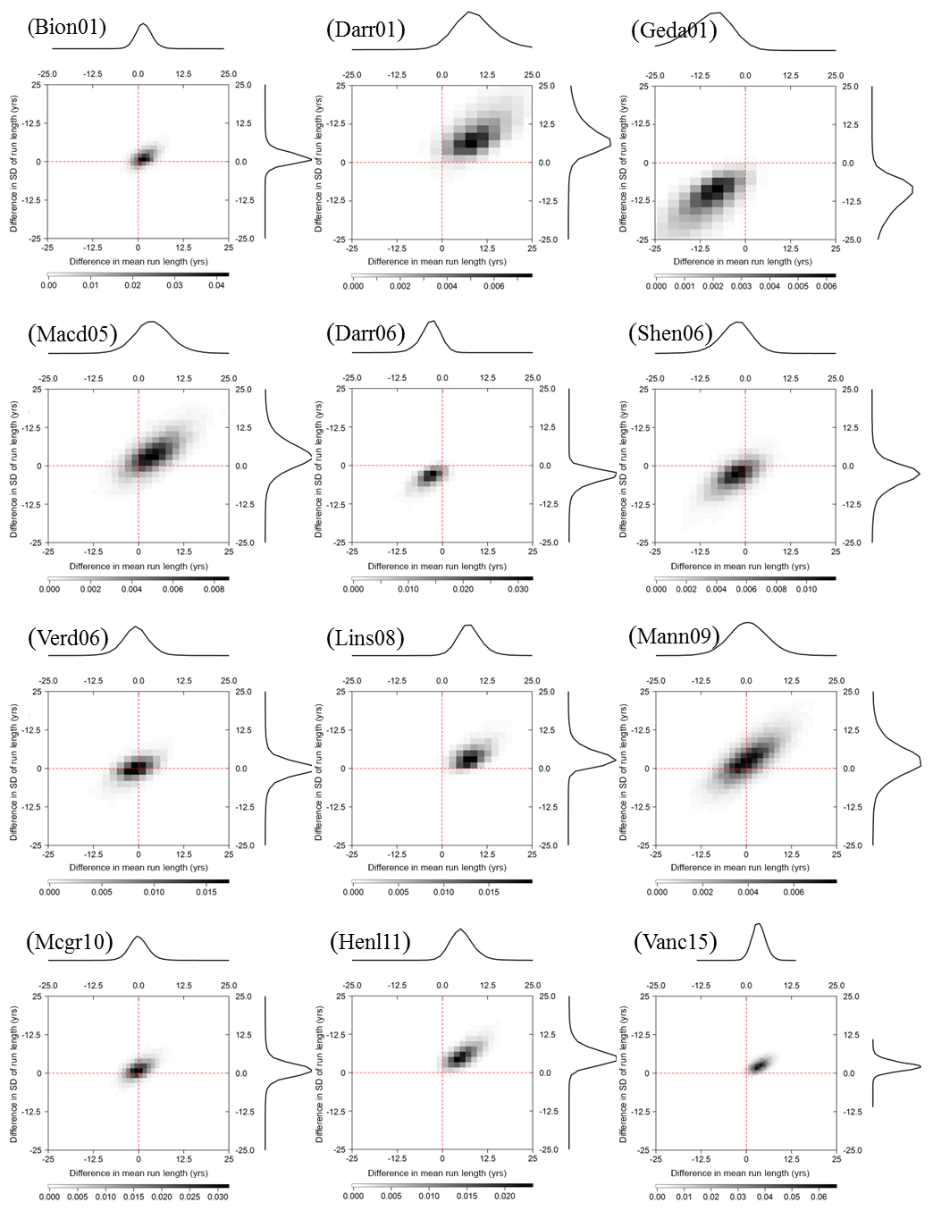
Figure 9Density and scatter plots of the differences between mean and standard deviation of positive and negative run length simulations (positive minus negative).
Henley et al. (2011) adopted the Gamma distribution as the probability model of PDV run lengths. The Gamma distribution has two parameters which are related to the mean μ and standard deviation σ of the run lengths. For each reconstruction, the positive and negative runs are extracted and the posterior distribution of the mean and standard deviation is inferred using MCMC (Gelman and Rubin, 1992). Figure 9 presents the joint posterior distribution of the differences in mean ( and standard deviation ( for each reconstruction. If the difference between positive and negative runs is statistically significant, one would expect the posterior distribution to be well removed from the zero-difference origin.
Inspection of Fig. 9 suggests there is no strong and consistent evidence to reject the assumption that positive and negative phase run length distributions are the same. Although the mean of positive phase run lengths tends to be longer than negative phase run lengths in several reconstructions (e.g. Vanc15, Henl11, Lins08, Darr01), the statistical significance of this difference is weak and the phenomenon is not consistent across all reconstructions. A similar conclusion applies to the standard deviation of positive and negative phase run lengths. This highlights the fundamental limitation of the small PDV run samples derived from the reconstructions.
4.2 Are run lengths stationary over the last millennium?
With paleoclimate reconstructions becoming longer, questions arise as to whether the PDV run length has been stationary in the past millennium and whether a shorter paleoclimate reconstruction is representative of the full range of variability that has occurred in the past or of what is plausible in the future. The stationarity issue has been explored in most PDV reconstructions used in this study. Biondi et al. (2001) identified weakened amplitude of bi-decadal oscillations in the late 1700s to mid-1800s. Based on reconstruction over 1700–1979, D'Arrigo et al. (2001) declared that variations at around 12–17 years are considerably more pronounced from 1700–1849 relative to 1850–1979, with a shift towards decreased amplitude since about 1850. Using visual inspection, Gedalof and Smith (2001) stated that the 30–70-year PDV frequency is confined to the pre-1840 portion of the series over the period of 1599–1983. D'Arrigo and Wilson (2006) reported a broad range of lower (multi-decadal to centennial) frequencies over the 1565–1988 period. Shen et al. (2006) pointed out that the major PDO regime timescale modes of oscillation have not been persistent over 1470–1998 and that 75–115-year and 50–70-year oscillations dominated the periods before and after 1850, respectively. Linsley et al. (2008) argued that decadal to inter-decadal variability in the South Pacific convergence zone region has been relatively constant over 1650–2004. MacDonald and Case (2005) presented evidence for a strong and persistent negative PDO state during the medieval period (900 to 1300 CE), suggesting a cool northeastern Pacific at that time. Mann et al. (2009) observed that the Little Ice Age (1400 to 1700) and the Medieval Climate Anomaly (950 to 1250) showed extra variability and persistence, challenging the assumption of a stationary climate in the past millennium. The mechanism responsible for the extra variability and persistence in studies by MacDonald and Case (2005) and Mann et al. (2009) is unclear and may be explained by centennial climate variability. It is unknown whether the PDV structure in the past millennium has remained stationary during periods that display extra variability and persistence. This issue can be investigated by filtering out the centennial trends.
All the above stationarity studies are based on single reconstructions. A further complication arises for reconstructions that only cover the last ∼300–400 years where the underlying non-stationarity may be masked as a consequence of sampling variability or the sampling variability is misinterpreted as non-stationarity. To mitigate this, here we use only millennium-length records, Macd05 (993–1996), Mann09 (500–2006) and Vanc15 (1000–2003), in an attempt to obtain statistically meaningful conclusions on PDV stationarity. The millennium-length records are split into pre-1600 and post-1600 samples to explore whether run length characteristics are statistically similar in these two periods and to shed light on whether shorter records (either the ∼100 year instrumental record or the 300–400-year paleoclimate reconstructions) are able to represent the full range of variability. The year 1600 is selected as the change point because most of the shorter PDV reconstructions date back to ∼1600 (refer to Table 1 and Fig. 2 for details).
Figure 10 presents box plots of pre-1600 and post-1600 run lengths: panel (a) presents box plots of pooled pre-1600 and post-1600 run lengths, while panel (b) shows box plots of pre-1600 and post-1600 runs for each of the three millennium-length reconstructions. A consistent pattern emerges in which the median run length and interquartile range are greater in the pre-1600 period for both pooled samples (Fig. 10a) and each individual reconstruction (Fig. 10b).
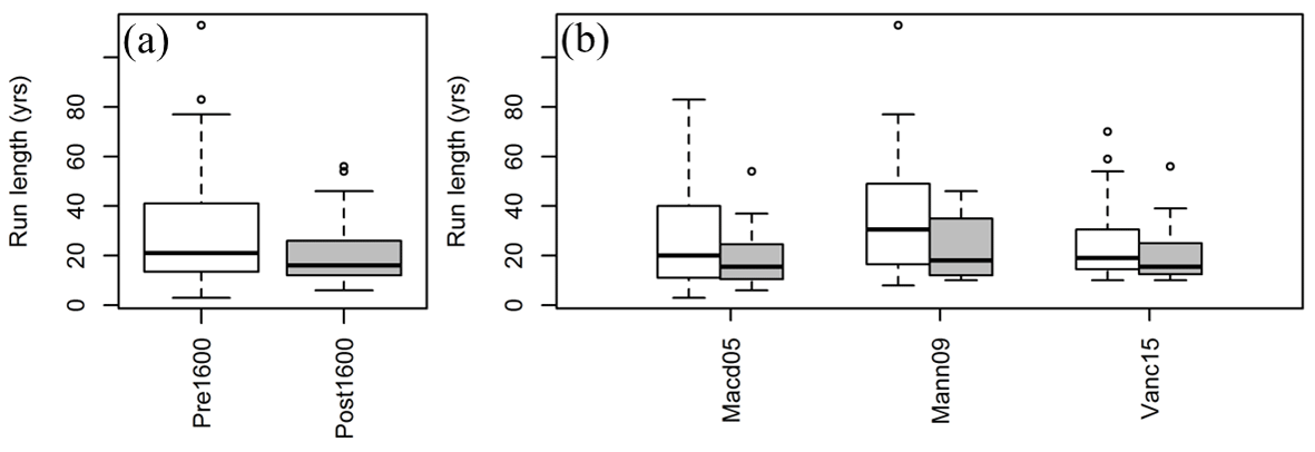
Figure 10Box plot of run length samples from different reconstructions (white box indicates pre-1600 and grey box indicates post-1600): (a) pooled run lengths from all three reconstructions; (b) run lengths for each reconstruction.
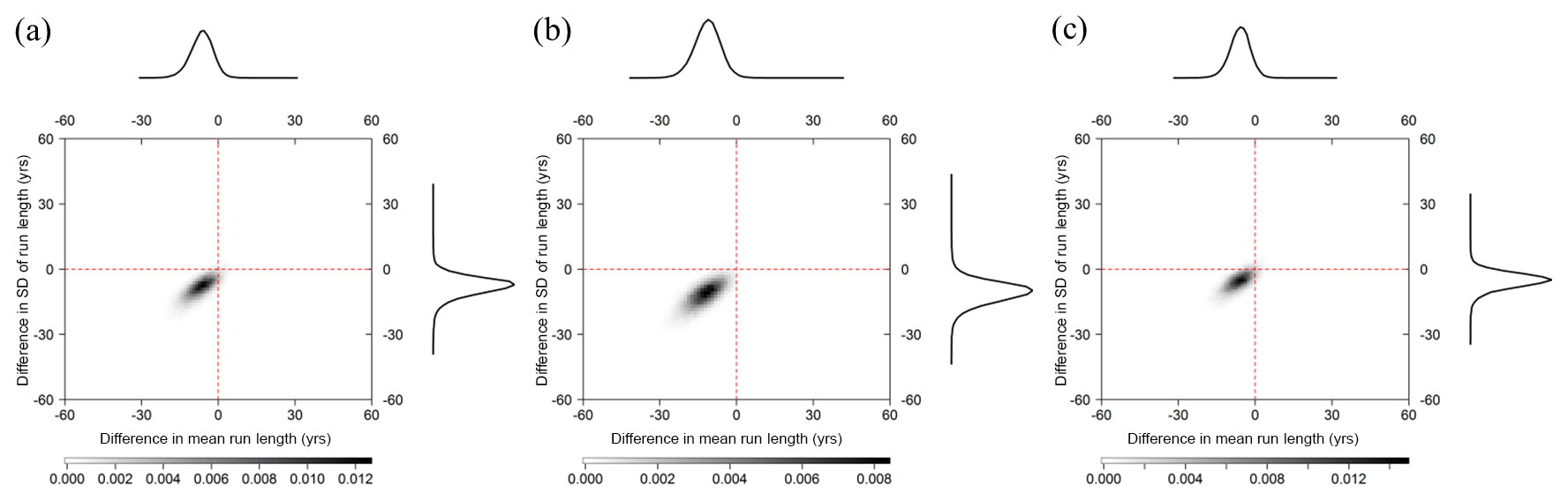
Figure 11Density and scatter plots of the differences between mean and standard deviation of pre-1600 and post-1600 run length simulations (post-1600 minus pre-1600): (a) Macd05, (b) Mann09, (c) Vanc15.
Bearing in mind that the samples are small, a Gamma distribution was inferred for the pre- and post-1600 samples. Figure 11 presents the joint posterior distribution of the differences in the pre- and post-1600 means and standard deviations for each reconstruction using all run lengths. A consistent pattern once again emerges. For all three reconstructions the posteriors of the pre- and post-1600 differences lie in the lower left quadrant with the origin minimally intersecting with the posterior. Therefore, the evidence that there is a difference is visually strong.
4.3 Discussion
All of the reconstructions reported in Table 1 did not distinguish between positive and negative PDV runs in their analysis, except for Vance et al. (2015). Based on a millennium IPO reconstruction, Vance et al. (2015) found that IPO has an average positive phase (IPO > 0.5) duration of 14 years and a negative phase (IPO < −0.5) duration of 9 years over 1000–2003 CE, and concluded that positive and negative phases durations and frequencies were different in the last millennium. This is the first study that addresses positive and negative PDV runs separately. However, based on comparisons with other reconstructions our results show that there remains uncertainty as to whether or not the run lengths of positive epochs are statistically different to the run length of negative epochs. It is important to keep in mind that the analysis here is fundamentally limited by small PDV run length sample sizes from most of the reconstructions. Two theories may explain the absence of a consistent difference between positive and negative run distributions. One is that no statistically meaningful differences exist and the other is that differences do exist but are masked by sampling variability. The latter seems plausible given the average number of phases (either positive or negative) per reconstruction are only 13.
All three millennium-length records lead to higher inferred run length mean and standard deviation in the pre-1600 samples, suggesting longer and more varied PDV runs during the period before 1600 AD. The fact that the differences in the mean and standard deviation of run lengths pre- and post-1600 appear to be statistically significant raises an important question, should the information from pre-1600 reconstructions be used to infer PDV behaviour in the near-future climate. If one adopts a gradualist view of climate non-stationarity, the immediate past would be considered more representative of the present than the more distant past. Setting aside for the moment the possibility that the climate–proxy relationship may be not be stationary, the gradualist perspective would support discarding the information from the pre-1600 reconstruction on the grounds that it introduces bias when inferring a statistical model of near climate PDV runs. We offer two reasons opposing this perspective.
First, there is no assurance that climate non-stationarity evolves in a gradual manner so that PDV behaviour in the near climate is better represented by the post-1600 climate than the pre-1600 climate. Indeed there is evidence to the contrary, namely that non-stationarity may be characterized by seemingly shorter-term shifts. Ho et al. (2017) found that American streamflow in the 20th century featured longer wet and dry spells compared to the preceding 450 years, suggesting the possibility of the occurrence of extended dry or wet periods in the future that exceeds variability presented in instrumental and short (i.e. < 500 years) paleoclimate reconstructions. Similar conclusions are also drawn in other studies (Vance et al., 2015; Tozer et al., 2016; Ho et al., 2015a, b).
Second, the inclusion of pre-1600 records offers a significantly larger sample of run lengths and therefore is more likely to capture the full range of what is plausible. Extended wet or dry periods considered as rare and extreme (or even impossible) based on recent (i.e. instrumental) history might actually be more likely than thought (or even common) when put into the context of climate conditions seen over the last 1000–2000 years. Even if one accepts the gradualist view of non-stationarity, the increased information about PDV more than outweighs the potential bias arising from the use of an apparently statistically inconsistent record.
It is therefore clear that in addition to short instrumental records inadequately sampling the length and severity of dry and wet epochs, the shorter paleoclimate reconstructions may similarly misrepresent hydroclimatic variability and persistence. For instance, from Ho et al. (2015a), when using the period 1684–1980, both the driest and wettest instrumental decadal rainfall lies closer to the middle of the minimum and maximum decadal reconstructed rainfall range. However, using the same method, Ho et al. (2015a) found that when 2751 years of reconstructions were examined, the wettest instrumental decadal rainfall is near the bottom of the maximum decadal reconstructed rainfall range, while the driest instrumental decadal rainfall is near the top of the minimum decadal reconstructed rainfall range. This suggests that statistics inferred from either instrumental data or short paleoclimate reconstructions will underestimate the variability contained in the longer paleoclimate reconstructions. Therefore, research focused on developing and analysing information about hydroclimatic conditions over the last 1000 years or more (e.g. multi-millennium paleoclimate reconstructions) is critical if we are to better understand, quantify and manage the full range of hydroclimatic variability, and associated risks, that are possible in the future.
This study is affected by two fundamental limitations. One is the small PDV run sample size from the reconstructions. For instance, the average number of phases (either positive or negative) per reconstruction are only 13. Another limitation is that all statistical signatures are based on paleoclimate reconstructions. Although multiple reconstructions are used, this study is constrained by the intrinsic limitations of paleoclimate reconstruction-based interpretations, such as assumptions of the stationarity of the proxy–climate relationship (Phipps et al., 2013). The possibility that all these reconstructions are biased in the same direction cannot be ruled out and as such conclusions based on multiple reconstructions may also be biased.
PDV, and associated run lengths of predominantly dry or wet conditions, has profound implications for precipitation and streamflow prediction, flood and drought risk assessment, and water resource management. Therefore, a better understanding of the statistical characteristics of PDV is needed. However, because instrumental records are short (∼100 years at best in Australia), there is considerable uncertainty about the key statistical signatures of PDV, including run lengths. Paleoclimate reconstructions, serving as a vehicle to provide longer realizations of PDV, have been widely studied and used. However, for various reasons (e.g. proxy sources, site locations, proxy resolutions, reconstruction methods and local non-PDV effects) temporal coherence between different reconstructions varies significantly (Kipfmueller et al., 2012). Hence, one PDV reconstruction may lead to significantly different conclusions from another reconstruction.
The aim of this paper was to explore the characteristics of key statistical signatures of PDV based on multiple PDV reconstructions. We focused on the duration of dry or wet hydrological epochs (i.e. run lengths) as the key statistical signature and developed a robust method for extracting run lengths from multiple reconstructions. Extracting run lengths objectively is challenging, given interactions with sources of variability on a variety of temporal and spatial scales. For instance, when millennium-length reconstructions are used, variability and persistence at the centennial scale can lead to biased characterization of decadal climate variability. The dynamic threshold framework introduced in this study, which takes centennial trends into consideration, was shown to extract meaningful run length information from multiple reconstructions.
No strong evidence was found to support the assumption that run lengths have statistically different distributions during positive and negative PDV phases. Analysis based on three millennium-long reconstructions suggests that it is more likely than not that PDV run length has been non-stationarity in the past millennium. This again highlights that the instrumental record (∼100 years at best), and even short paleoclimate reconstructions (i.e. less than 400 years into the past), should not be assumed to represent the full range of variability that has occurred in the past or what may occur in the future. Caution should be exercised regarding assumptions that the climate is stationary and the implications of a non-stationary climate should at least be tested. Longer climate reconstructions (i.e. 1000 years or more) appear to give more useful information and insights into what has occurred in the past and also tell us more about what is plausible and what needs to be planned for in the future.
All of the reconstructions explored in this study have focused on the run length of PDV, yet they have provided quite different run length characterizations. This again highlights that each reconstruction is subject to errors, both random and systematic, that are not fully understood. Therefore, a challenging and important research direction is the analysis of run length characteristics with explicit consideration of the errors. Another important research direction is the continued refinement of methods that utilize PDV information in water resource management as we work toward improving how we assess and manage hydrological risks in a variable and changing climate.
The unfiltered instrumental PDO index can be accessed through http://research.jisao.washington.edu/pdo/PDO.latest.txt (last access: 22 September 2016; Mantua et al., 1997; Zhang et al., 1997). Data of the reconstruction Bion01 can be accessed from ftp://ftp.ncdc.noaa.gov/pub/data/paleo/treering/reconstructions/pdo.txt (last access: 22 September 2016; Biondi et al., 2001). Data of the reconstruction Darr01 can be obtained from ftp://ftp.ncdc.noaa.gov/pub/data/paleo/treering/reconstructions/pdo-darrigo2001.txt (last access: 22 September 2016; D'Arrigo et al., 2001). Data of the reconstruction Geda01 are currently not freely available; requests should be directed to smith@uvic.ca (Gedalof and Smith, 2001). Data of the reconstruction Lins08 can be accessed through https://www.ncdc.noaa.gov/paleo-search/study/6216?siteId=56368 (last access: 22 September 2016; Linsley et al., 2008). Data of the reconstruction Mann09 can be obtained from http://science.sciencemag.org/content/326/5957/1256/tab-figures-data (last access: 22 September 2016; Mann et al., 2009). Data of the reconstruction Mcgr10 can be obtained from https://www.ncdc.noaa.gov/paleo-search/study/8732 (last access: 22 September 2016; McGregor et al., 2010). Data of the reconstruction Vanc15 can be obtained from Vance et al. (2015).
LZ has contributed to most of the development of methods, analysis and writing of the paper. GK and ASK have contributed to assisting with analysis, writing, reviewing and revising the paper, and GW has contributed to writing and reviewing the paper.
The authors declare that they have no conflict of interest.
Funding for this research was provided by Australian Research Council Linkage
Grant LP120200494 with further funding and/or in-kind support also provided
by the NSW Office of Environment and Heritage, Sydney Catchment Authority,
Hunter Water Corporation, NSW Office of Water, and NSW Department of Finance
and Services.
Edited by: Thomas Kjeldsen
Reviewed by: two anonymous referees
Andreoli, R. V. and Kayano, M. T.: ENSO-related rainfall anomalies in South America and associated circulation features during warm and cold Pacific decadal oscillation regimes, Int. J. Climatol., 25, 2017–2030, https://doi.org/10.1002/joc.1222, 2005.
Atwood, A. R., Wu, E., Frierson, D. M. W., Battisti, D. S., and Sachs, J. P.: Quantifying Climate Forcings and Feedbacks over the Last Millennium in the CMIP5–PMIP3 Models, J. Climate, 29, 1161–1178, https://doi.org/10.1175/JCLI-D-15-0063.1, 2015.
Biondi, F., Gershunov, A., and Cayan, D. R.: North Pacific decadal climate variability since 1661, J. Climate, 14, 5–10, https://doi.org/10.1175/1520-0442(2001)014<0005:NPDCVS>2.0.CO;2, 2001.
Chiew, F. H. S.: Estimation of rainfall elasticity of streamflow in Australia, Hydrolog. Sci. J., 51, 613–625, https://doi.org/10.1623/hysj.51.4.613, 2006.
Cook, B. I., Smerdon, J. E., Seager, R., and Cook, E. R.: Pan-Continental Droughts in North America over the Last Millennium, J. Climate, 27, 383–397, https://doi.org/10.1175/JCLI-D-13-00100.1, 2013.
D'Arrigo, R., Villalba, R., and Wiles, G.: Tree-ring estimates of Pacific decadal climate variability, Clim. Dynam., 18, 219–224, https://doi.org/10.1007/s003820100177, 2001.
D'Arrigo, R. and Wilson, R.: On the Asian expression of the PDO, Int. J. Climatol., 26, 1607–1617, https://doi.org/10.1002/joc.1326, 2006.
Dai, A.: The influence of the inter-decadal Pacific oscillation on US precipitation during 1923–2010, Clim. Dynam., 41, 633–646, https://doi.org/10.1007/s00382-012-1446-5, 2013.
Dong, B. and Dai, A.: The influence of the Interdecadal Pacific Oscillation on Temperature and Precipitation over the Globe, Clim. Dynam., 45, 2667–2681, https://doi.org/10.1007/s00382-015-2500-x, 2015.
Folland, C. K., Renwick, J. A., Salinger, M. J., and Mullan, A. B.: Relative influences of the interdecadal Pacific oscillation and ENSO on the South Pacific convergence zone, Geophys. Res. Lett., 29, 1643, https://doi.org/10.1029/2001GL014201, 2002.
Gedalof, Z. and Smith, D. J.: Interdecadal climate variability and regime-scale shifts in Pacific North America, Geophys. Res. Lett., 28, 1515–1518, https://doi.org/10.1029/2000GL011779, 2001.
Gelman, A. and Rubin, D. B.: Inference from Iterative Simulation Using Multiple Sequences, Stat. Sci., 7, 457–472, https://doi.org/10.1214/ss/1177011136, 1992.
Goodrich, G. B. and Walker, J. M.: The Influence of the PDO on Winter Precipitation During High- and Low-Index ENSO Conditions in the Eastern United States, Phys. Geogr., 32, 295–312, https://doi.org/10.2747/0272-3646.32.4.295, 2011.
Henley, B. J.: Pacific decadal climate variability: Indices, patterns and tropical-extratropical interactions, Global Planet. Change, 155, 42–55, https://doi.org/10.1016/j.gloplacha.2017.06.004, 2017.
Henley, B. J., Thyer, M. A., Kuczera, G., and Franks, S. W.: Climate-informed stochastic hydrological modeling: Incorporating decadal-scale variability using paleo data, Water Resour. Res., 47, W11509, https://doi.org/10.1029/2010WR010034, 2011.
Henley, B. J., Thyer, M. A., and Kuczera, G.: Climate driver informed short-term drought risk evaluation, Water Resour. Res., 49, 2317–2326, https://doi.org/10.1002/wrcr.20222, 2013.
Henley, B., Gergis, J., Karoly, D., Power, S., Kennedy, J., and Folland, C.: A Tripole Index for the Interdecadal Pacific Oscillation, Clim. Dynam., 45, 1–14, https://doi.org/10.1007/s00382-015-2525-1, 2015.
Henley, B. J., Meehl, G., Power, S., Folland, C., King, A., Brown, J., Karoly, D., Delage, F., Gallant, A., and Freund, M.: Spatial and temporal agreement in climate model simulations of the interdecadal pacific oscillation, Environ. Res. Lett., 12, 044011, https://doi.org/10.1088/1748-9326/aa5cc8, 2017.
Ho, M., Kiem, A. S., and Verdon-Kidd, D. C.: A paleoclimate rainfall reconstruction in the Murray-Darling Basin (MDB), Australia: 2. Assessing hydroclimatic risk using paleoclimate records of wet and dry epochs, Water Resour. Res., 51, 8380–8396, https://doi.org/10.1002/2015WR017059, 2015a.
Ho, M., Kiem, A. S., and Verdon-Kidd, D. C.: A paleoclimate rainfall reconstruction in the Murray-Darling Basin (MDB), Australia: 1. Evaluation of different paleoclimate archives, rainfall networks, and reconstruction techniques, Water Resour. Res., 51, 8362–8379, https://doi.org/10.1002/2015WR017058, 2015b.
Ho, M., Lall, U., Sun, X., and Cook, E. R.: Multiscale temporal variability and regional patterns in 555 years of conterminous U.S. streamflow, Water Resour. Res., 3047–3066, https://doi.org/10.1002/2016WR019632, 2017.
Hoell, A. and Funk, C.: Indo-Pacific sea surface temperature influences on failed consecutive rainy seasons over eastern Africa, Clim. Dynam., 43, 1645–1660, https://doi.org/10.1007/s00382-013-1991-6, 2014.
Hu, Z.-Z. and Huang, B.: Interferential Impact of ENSO and PDO on Dry and Wet Conditions in the U.S. Great Plains, J. Climate, 22, 6047–6065, https://doi.org/10.1175/2009JCLI2798.1, 2009.
Kiem, A. S. and Franks, S. W.: Multi-decadal variability of drought risk, eastern Australia, Hydrol. Process., 18, 2039–2050, https://doi.org/10.1002/hyp.1460, 2004.
Kiem, A. S., Franks, S. W., and Kuczera, G.: Multi-decadal variability of flood risk, Geophys. Res. Lett., 30, 1035, https://doi.org/10.1029/2002GL015992, 2003.
Kipfmueller, K. F., Larson, E. R., and St. George, S.: Does proxy uncertainty affect the relations inferred between the Pacific Decadal Oscillation and wildfire activity in the western United States?, Geophys. Res. Lett., 39, PA2219, https://doi.org/10.1029/2011GL050645, 2012.
Kirtman, B., Power, S. B., Adedoyin, A. J., Boer, G. J., Bojariu, R., Camilloni, I., Doblas-Reyes, F., Fiore, A. M., Kimoto, M., and Meehl, G.: Near-term climate change: projections and predictability, in: Climate Change 2013: The Physical Science Basis. Contribution of Working Group I to the Fifth Assessment Report of the Intergovernmental Panel on Climate Change, Cambridge University Press, Cambridge,United Kingdom and New York, NY, USA, 953–1028, 2013.
Krishnan, R. and Sugi, M.: Pacific decadal oscillation and variability of the Indian summer monsoon rainfall, Clim. Dynam., 21, 233–242, https://doi.org/10.1007/s00382-003-0330-8, 2003.
Li, L., Li, W., and Kushnir, Y.: Variation of the North Atlantic subtropical high western ridge and its implication to Southeastern US summer precipitation, Clim. Dynam., 39, 1401–1412, https://doi.org/10.1007/s00382-011-1214-y, 2012.
Linsley, B. K., Zhang, P., Kaplan, A., Howe, S. S., and Wellington, G. M.: Interdecadal-decadal climate variability from multicoral oxygen isotope records in the South Pacific Convergence Zone region since 1650 AD, Paleoceanography, 23, PA2219, https://doi.org/10.1029/2007PA001539, 2008.
Ma, Z.: The interdecadal trend and shift of dry/wet over the central part of North China and their relationship to the Pacific Decadal Oscillation (PDO), Chinese Sci. Bull., 52, 2130–2139, https://doi.org/10.1007/s11434-007-0284-z, 2007.
MacDonald, G. M. and Case, R. A.: Variations in the Pacific Decadal Oscillation over the past millennium, Geophys. Res. Lett., 32, L08703, https://doi.org/10.1029/2005GL022478, 2005.
Mann, M. E., Zhang, Z., Rutherford, S., Bradley, R. S., Hughes, M. K., Shindell, D., Ammann, C., Faluvegi, G., and Ni, F.: Global signatures and dynamical origins of the Little Ice Age and Medieval Climate Anomaly, Science, 326, 1256–1260, https://doi.org/10.1126/science.1177303, 2009.
Mantua, N. J. and Hare, S. R.: The Pacific decadal oscillation, J. Oceanogr., 58, 35–44, https://doi.org/10.1023/a:1015820616384, 2002.
Mantua, N. J., Hare, S. R., Zhang, Y., Wallace, J. M., and Francis, R. C.: A Pacific interdecadal climate oscillation with impacts on salmon production, B. Am. Meteorol. Soc., 78, 1069–1079, https://doi.org/10.1175/1520-0477(1997)078<1069:APICOW>2.0.CO;2, 1997.
Mauget, S. A.: Multidecadal regime shifts in US streamflow, precipitation, and temperature at the end of the twentieth century, J. Climate, 16, 3905–3916, https://doi.org/10.1175/1520-0442(2003)016<3905:MRSIUS>2.0.CO;2, 2003.
McCabe, G. J., Ault, T. R., Cook, B. I., Betancourt, J. L., and Schwartz, M. D.: Influences of the El Niño Southern Oscillation and the Pacific Decadal Oscillation on the timing of the North American spring, Int. J. Climatol., 32, 2301–2310, https://doi.org/10.1002/joc.3400, 2012.
McGregor, S., Timmermann, A., and Timm, O.: A unified proxy for ENSO and PDO variability since 1650, Clim. Past, 6, 1–17, https://doi.org/10.5194/cp-6-1-2010, 2010.
Mehta, V. M., Rosenberg, N. J., and Mendoza, K.: Simulated Impacts of Three Decadal Climate Variability Phenomena on Water Yields in the Missouri River Basin1, J. Am. Water Resour. As., 47, 126–135, https://doi.org/10.1111/j.1752-1688.2010.00496.x, 2011.
Micevski, T., Franks, S. W., and Kuczera, G.: Multidecadal variability in coastal eastern Australian flood data, J. Hydrol., 327, 219–225, https://doi.org/10.1016/j.jhydrol.2005.11.017, 2006.
Parker, D., Folland, C., Scaife, A., Knight, J., Colman, A., Baines, P., and Dong, B.: Decadal to multidecadal variability and the climate change background, J. Geophys. Res.-Atmos., 112, D18115, https://doi.org/10.1029/2007JD008411, 2007.
Peng, Y., Shen, C., Cheng, H., and Xu, Y.: Simulation of the Interdecadal Pacific Oscillation and its impacts on the climate over eastern China during the last millennium, J. Geophys. Res.-Atmos., 120, 7573–7585, https://doi.org/10.1002/2015JD023104, 2015.
Phipps, S. J., McGregor, H. V., Gergis, J., Gallant, A. J. E., Neukom, R., Stevenson, S., Ackerley, D., Brown, J. R., Fischer, M. J., and Van Ommen, T. D.: Paleoclimate data–model comparison and the role of climate forcings over the past 1500 years, J. Climate, 26, 6915–6936, https://doi.org/10.1175/JCLI-D-12-00108.1, 2013.
Power, S., Casey, T., Folland, C., Colman, A., and Mehta, V.: Inter-decadal modulation of the impact of ENSO on Australia, Clim. Dynam., 15, 319–324, https://doi.org/10.1007/s003820050284, 1999.
Razavi, S., Elshorbagy, A., Wheater, H., and Sauchyn, D.: Toward understanding nonstationarity in climate and hydrology through tree ring proxy records, Water Resour. Res., 51, 1813–1830, https://doi.org/10.1002/2014WR015696, 2015.
Reason, C. J. C. and Rouault, M.: ENSO-like decadal variability and South African rainfall, Geophys. Res. Lett., 29, 16-11–16-14, https://doi.org/10.1029/2002GL014663, 2002.
Saft, M., Western, A. W., Zhang, L., Peel, M. C., and Potter, N. J.: The influence of multiyear drought on the annual rainfall-runoff relationship: An Australian perspective, Water Resour. Res., 51, 2444–2463, https://doi.org/10.1002/2014WR015348, 2015.
Shen, C., Wang, W. C., Gong, W., and Hao, Z.: A Pacific Decadal Oscillation record since 1470 AD reconstructed from proxy data of summer rainfall over eastern China, Geophys. Res. Lett., 33, L03702, https://doi.org/10.1029/2005GL024804, 2006.
Tozer, C. R., Vance, T. R., Roberts, J. L., Kiem, A. S., Curran, M. A. J., and Moy, A. D.: An ice core derived 1013-year catchment-scale annual rainfall reconstruction in subtropical eastern Australia, Hydrol. Earth Syst. Sci., 20, 1703–1717, https://doi.org/10.5194/hess-20-1703-2016, 2016.
Vance, T. R., Roberts, J. L., Plummer, C. T., Kiem, A. S., and van Ommen, T. D.: Interdecadal Pacific variability and eastern Australian megadroughts over the last millennium, Geophys. Res. Lett., 42, 129–137, https://doi.org/10.1002/2014GL062447, 2015.
Verdon, D. C., Wyatt, A. M., Kiem, A. S., and Franks, S. W.: Multidecadal variability of rainfall and streamflow: Eastern Australia, Water Resour. Res., 40, W10201, https://doi.org/10.1029/2004WR003234, 2004.
Verdon, D. C. and Franks, S. W.: Long-term behaviour of ENSO: Interactions with the PDO over the past 400 years inferred from paleoclimate records, Geophys. Res. Lett., 33, L06712, https://doi.org/10.1029/2005GL025052, 2006.
von Storch, H., Zorita, E., Jones, J. M., Gonzalez-Rouco, F., and Tett, S. F. B.: Response to Comment on “Reconstructing Past Climate from Noisy Data”, Science, 312, 529, https://doi.org/10.1126/science.1121571, 2006.
Wahl, E. R., Ritson, D. M., and Ammann, C. M.: Comment on “Reconstructing Past Climate from Noisy Data”, Science, 312, 529, https://doi.org/10.1126/science.1120866, 2006.
Wang, S., Huang, J., He, Y., and Guan, Y.: Combined effects of the Pacific Decadal Oscillation and El Niño-Southern Oscillation on Global Land Dry–Wet Changes, Sci. Rep. UK, 4, 6651, https://doi.org/10.1038/srep06651, 2014.
Wu, Z., Huang, N. E., Long, S. R., and Peng, C.-K.: On the trend, detrending, and variability of nonlinear and nonstationary time series, P. Natl. Acad. Sci., 104, 14889–14894, https://doi.org/10.1073/pnas.0701020104, 2007.
Zhang, Y., Wallace, J. M., and Battisti, D. S.: ENSO-like interdecadal variability: 1900–93, J. Climate, 10, 1004–1020, https://doi.org/10.1175/1520-0442(1997)010<1004:ELIV>2.0.CO;2, 1997.