the Creative Commons Attribution 3.0 License.
the Creative Commons Attribution 3.0 License.
A discrete wavelet spectrum approach for identifying non-monotonic trends in hydroclimate data
Yan-Fang Sang
Fubao Sun
Vijay P. Singh
The hydroclimatic process is changing non-monotonically and identifying its trends is a great challenge. Building on the discrete wavelet transform theory, we developed a discrete wavelet spectrum (DWS) approach for identifying non-monotonic trends in hydroclimate time series and evaluating their statistical significance. After validating the DWS approach using two typical synthetic time series, we examined annual temperature and potential evaporation over China from 1961–2013 and found that the DWS approach detected both the “warming” and the “warming hiatus” in temperature, and the reversed changes in potential evaporation. Further, the identified non-monotonic trends showed stable significance when the time series was longer than 30 years or so (i.e. the widely defined “climate” timescale). The significance of trends in potential evaporation measured at 150 stations in China, with an obvious non-monotonic trend, was underestimated and was not detected by the Mann–Kendall test. Comparatively, the DWS approach overcame the problem and detected those significant non-monotonic trends at 380 stations, which helped understand and interpret the spatiotemporal variability in the hydroclimatic process. Our results suggest that non-monotonic trends of hydroclimate time series and their significance should be carefully identified, and the DWS approach proposed has the potential for wide use in the hydrological and climate sciences.


Climate and hydrological processes are exhibiting great variability (Allen and Ingram, 2002; Trenberth et al., 2014). Quantitatively identifying changing signals in the hydroclimate process is of great socioeconomic significance (Diffenbaugh et al., 2008; Stocker et al., 2013) as an important basis for hydrological modelling, understanding the future hydroclimatic regimes, and water resources planning and management. However, it remains a challenge to both scientific and social communities. The simplest and the most straightforward way to identify changes in the hydroclimate process would be to fit a monotonic (e.g. linear) trend at a certain time period at which a significance level would be assigned by a statistical test. Among the methods used for the detection of trends, the Mann–Kendall (MK) non-parametric test is most widely used and has been successfully applied in studies on climate change and its impact, when the time series is almost monotonic as required and a statistical threshold of ±1.96 is set to judge the significance of trends at the 95 % confidence level (Burn and Hag Elnur, 2002; Yue et al., 2002). However, due to its nonlinear and nonstationary nature, the hydroclimate process is changing and developing in a more complicated way compared to a monotonic trends on long timescales (Cohn and Lins, 2005; Milly et al., 2008). For example, a debate on the recent change in global air temperature has been receiving enormous public and scientific attention. This global air temperature increase during 1980–1998, passing most statistical significance tests and has since stabilized until now, is widely called the “global warming hiatus” (Kosaka and Xie, 2013; Roberts et al., 2015; Medhaug et al., 2017). Another known example is the “evaporation paradox” (Brutsaert and Parlange, 1998; Roderick and Farquhar, 2002), potential evaporation has declined worldwide from the 1960s, again passing most statistical significance tests, but then reversed after the 1990s. In practice, for hydroclimate time series, non-monotonicity is more the rule rather than the exception (Dixon et al., 2006; Adam and Lettenmaier, 2008; Gong et al., 2010). Therefore, identifying the non-monotonic trends hidden in those hydroclimate time series and assessing its statistical significance present a significant research task for understanding hydroclimatic variability and changes on long timescales.
Among those methods presently used in time series analysis, the wavelet method, including both continuous and discrete wavelet transforms, has the superior capability of handling nonstationary characteristics of the time series on multiple timescales (Percival and Walden, 2000; Labat, 2005); so it may also be more suitable for identifying non-monotonic trends in hydroclimate time series on long timescales. In a seminal work, Torrence and Compo (1998) placed the continuous wavelet transform in the framework of statistical analysis by formulating a significance test. Since then, the continuous wavelet method has become more applicable and rapidly developed to estimate the significance of variability in climate and hydrological studies. The continuous wavelet spectrum (i.e. continuous wavelet variance) was especially established to detect those significant variabilities in the hydroclimate process (Labat et al., 2000). However, in the continuous wavelet results of a time series, a known technical issue is “data redundancy” (Gaucherel, 2002; Nourani et al., 2014), which is the redundant information across timescales leading to more uncertainty.
On the contrary, the other type of wavelet transform, i.e. the discrete wavelet transform (DWT), has the potential to overcome that problem of data redundancy, in that those wavelets used for discrete wavelet transform must meet the orthogonal properties. Therefore, the discrete wavelet method can be more effective to identify and describe the non-monotonic trend in a time series (Almasri et al., 2008; de Artigas et al., 2006; Kallache et al., 2005; Partal and Kucuk, 2006; Nalley et al., 2012). However, there lacked an effective discrete wavelet spectrum in the wavelet methodology, without which uncertainty in the discrete wavelet-aided identification of a trend could not be accurately estimated and the significance level of the identified trend could not be quantitatively evaluated either. To overcome the problem, Sang et al. (2013) discussed the definition of trend, and proposed a discrete wavelet energy function method for the identification of trends, with the basic idea of comparing the difference of discrete wavelet results between hydrological data and noise. The method used a proper confidence interval to assess the statistical significance of the identified trend, in which the key equation for quantifying a trend's significance was based on the concept of quadratic sum. However, computation of the quadratic sum disobeys the customary practice of computing variance in spectral analysis. By using the quadratic sum, the significance of a non-monotonic trend cannot be reasonably assessed, because it neglects the large influence of a trend's mean value. For instance, for those trends with small variations but large mean values, the quadratic sums are large values, of which the statistical significance of trends would inevitably be overestimated. Therefore, evaluation of the statistical significance of a non-monotonic trend in a time series should be based on its own variability, and the influence of other factors should also be eliminated.
By combining the advantages of discrete wavelet transform and successful practice in spectral analysis methods, this study aims at developing a practical but reliable discrete wavelet spectrum (DWS) approach for identifying non-monotonic trends in hydroclimate time series and quantifying their statistical significance, and further improving the understanding of non-monotonic trends by investigating their variation with data length increase. To do that, Sect. 2 presents details of the newly developed approach building on the wavelet theory and spectrum analysis. In Sect. 3, we use both synthetic time series and annual time series of air temperature and potential evaporation over China as examples to investigate the applicability of the approach, which is followed by a discussion and conclusion in the final section.
Here we develop an approach, termed as the “discrete wavelet spectrum approach,” for identifying non-monotonic trends in hydroclimate time series, in which the discrete wavelet transform (DWT) is used first to separate the trend on long timescales, and its statistical significance is then evaluated by using the DWS, whose confidence interval is quantified and described through a Monte Carlo test.
Following the wavelet analysis theory (Percival and Walden, 2000), the DWT of a time series f(t) with a time order t can be expressed as
where ψ∗(t) is the complex conjugate of the mother wavelet ψ(t), a0 and b0 are constants, integer k is a time translation factor, and Wf(j,k) is the discrete wavelet coefficient under the decomposition level j (i.e. timescale . In practice, the dyadic DWT is used widely by assigning a0=2 and b0=1:
The highest decomposition level M is determined by the length L of series f(t), and can be calculated as log 2(L) (Foufoula-Georgiou and Kumar, 2014). The sub-signal fj(t) in the original series f(t) under each level j (j=1, 2, ..., M) can be reconstructed as
where the sub-signal fj(t) at the highest decomposition level (when j=M) defines and describes the non-monotonic trend of the series f(t), as generally understood. However, it should be noted that a meaningful trend closely depends on the timescale concerned. If the variability in series f(t) on a certain smaller timescale K (K < L) is concerned, the proper decomposition level can be determined as log 2(K), then the sum of all those sub-signals on the timescale equal to and bigger than K can be the non-monotonic trend identified.
Sang (2012) discussed the influence of the choice of mother wavelet and decomposition level, as well as noise types on the discrete wavelet decomposition of time series, and further proposed some methods to solve for them. By conducting Monte Carlo experiments, he found that the seven wavelet families (126 mother wavelets) used for DWT can be divided into three types, and recommended the first type, by which wavelet energy functions of diverse types of noise data remain stable and thus have little influence on the wavelet decomposition of time series. Specifically, one (a) chooses an appropriate wavelet, according to the relationship of statistical characteristics among the original series, de-noised series, and removed noise; (b) chooses a proper decomposition level by analysing the difference between energy functions of the analysed series and that of noise; (c) and then identifies the deterministic components (including trend) by conducting significance testing of the DWT. These methods are closely built on the composition and variability in hydroclimate time series on different timescales. They were used here to accurately identify and describe the non-monotonic trend in a time series, and assess its statistical significance.

Figure 1Technical flowchart for identification of the non-monotonic trends in a time series using the developed discrete wavelet spectrum (DWS) approach, where the discrete wavelet transform (DWT) method was used to decompose the time series and get sub-signal at each decomposition level (DL), and the reference discrete wavelet spectrum (RDWS) with certain confidence interval (CI) was used for the evaluation of significance.
Further, to establish a reliable DWS of time series, we need to specify a spectrum value E(j) for each sub-signal fj(t) (in Eq. 3), of which we can quantitatively evaluate its importance and statistical significance. Following the general practice in conventional spectral analysis methods (Fourier transform, maximum entropy spectral analysis, etc.), here we define E(j) at the jth level by taking the variance of fj(t):
This can accurately quantify the intensity of variation in sub-signals (including trend) by eliminating the influence of their mean values, which is different from the quadratic-sum-based method proposed by Sang et al. (2013). For hydroclimate time series, both stochastic and deterministic components generally have distinctive characteristics from purely noise components (Sang et al., 2012; Rajaram et al., 2015). Due to the grid of dyadic DWT (Partal and Cigizoglu, 2008), discrete wavelet spectra Er(j) of various noise types strictly follow an exponentially decreasing rule with a base 2 (Sang, 2012):
The DWSs of deterministic components and that of noise are obviously different. Hence, we define the DWS of noise data as the “reference discrete wavelet spectrum” (RDWS), of which we evaluate the statistical significance of the non-monotonic trend of a time series.
To be specific, we design a technical flowchart to show how we develop the DWS approach for identifying the non-monotonic trend of time series, and also for evaluating the statistical significance of that trend (see details in Fig. 1):
-
For the series f(t) with length L to be analysed, we normalize and decompose it using the DWT method in Eqs. (2) and (3);
-
We calculate the DWS of the series f(t) by using Eq. (4);
-
For comparison, we then use the Monte Carlo method to generate normalized noise data N with the same length as the series f(t), and compute its RDWS by using Eq. (4). Considering that DWSs of diverse types of noise data consistently follow Eq. (5), here we generate noise data following the standard normal probability distribution;
-
We repeat the above step 5000 times, and calculate the mean value and variance of the spectrum values (in Eq. 4) of the normalized noise data N at each decomposition level j. Based on it, we estimate an appropriate confidence interval of RDWS at the concerned confidence level. In this study, we considered the 95 % confidence level;
-
In comparing the DWS of the series f(t) and the confidence interval generated by that of noise (i.e. RDWS), we identified the deterministic components under the highest decomposition level as the non-monotonic trend of the series, and judged whether it was significant. Specifically, if the spectrum value of the analysed series' sub-signal under the highest level was above the confidence interval of RDWS, it was considered that the non-monotonic trend was statistically significant; otherwise, if the spectrum value of the sub-signal under the highest level fell into the confidence interval of RDWS, it was not statistically significant;
-
If a smaller timescale K is concerned, we can use the decomposition level log 2(K), instead of M, and then repeat steps (1–5) to identify the non-monotonic trend on that timescale.
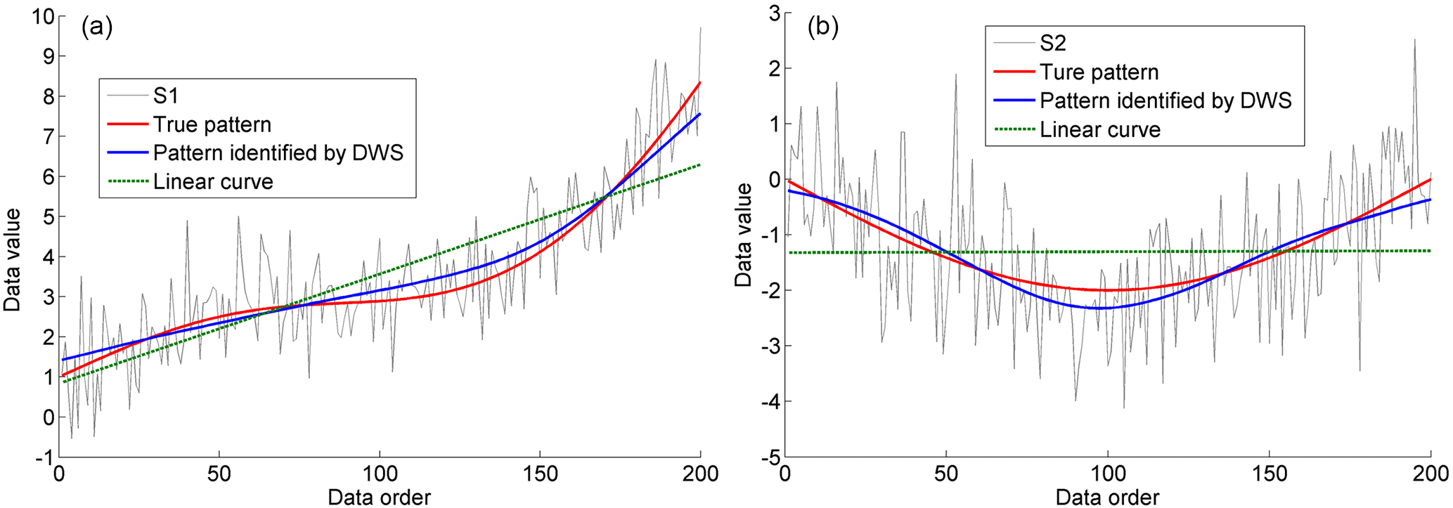
Figure 2Non-monotonic trends in the synthetic series S1 (a) and S2 (b) identified by the discrete wavelet spectrum (DWS) approach, and the linear trends in the two series. Synthetic series S1 is generated as and synthetic series S2 is generated as , where α is a random process following the standard normal distribution.
In the following section, we mainly investigate the applicability and reliability of the DWS approach for identifying the non-monotonic trend and assessing its significance, and further investigate the variation in non-monotonic trends with data length increase to improve our understanding of trends on long timescales.
3.1 Synthetic series analysis
To test and verify the reliability of the developed DWS approach for identifying the non-monotonic trends of a time series, we considered the general hydrological situations and generated two synthetic series data, with known signals and noise. For investigating the variation in non-monotonic trends with data length increase, we set the length of the two synthetic series as 200, and the noise in them followed a standard normal probability distribution. The first synthetic series S1 consisted of an exponentially increasing line and a periodic curve (with a periodicity of 200) with some noise content (Fig. 2a) and the second synthetic series S2 was generated by including a semi-sine curve, a periodic curve (with a periodicity of 50), and some noise content (Fig. 2b). Using the MK test and considering monotonic trends, series S1 showed a significant increase but the trend of series S2 was not significant.
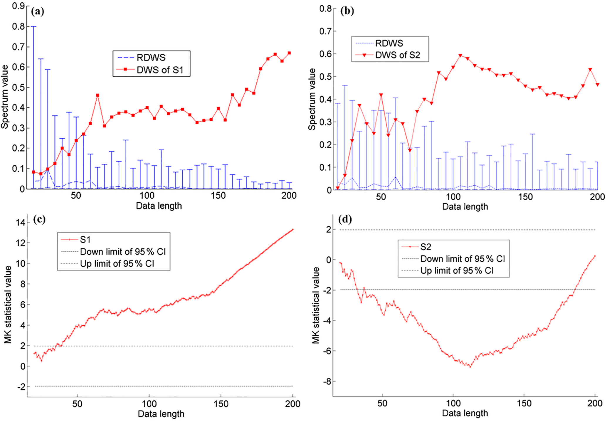
Figure 3Evaluation of statistical significance of non-monotonic trends in the synthetic series S1 (a) and S2 (b) with different data length by the discrete wavelet spectrum (DWS) approach, and the results by the Mann–Kendall (MK) test (c, d). In panels (a) and (b), the dashed blue line is the reference discrete wavelet spectrum (RDWS) with 95 % confidence interval under each data length; if the red data point at certain data length is above the blue bar, it is thought that the trend is significant at the 95 % confidence level. In panels (c) and (d), the two black dashed lines indicate the 95 % confidence interval (CI) with the thresholds of ±1.96 in the MK test.
When using the DWS approach (Fig. 1), we considered the timescale as data length, and used the Daubechies (db8) wavelet to decompose series S1 into seven (i.e. < log 2200) sub-signals using Eqs. (2) and (3). Then we took the sub-signals under the seventh level as the defined non-monotonic trend. As shown in Fig. 2a, the identified non-monotonic trend in series S1 was similar to the true trend. However, the linear fitting curve (a monotonic curve) could not capture the detail of the non-monotonic trend. The same approach was applied to series S2 in Fig. 2b and the conclusion did not change. Moreover, for series S2 with large variability on long timescales, the linear fitting curve or other monotonic curves may not be physically meaningful.
We computed the DWSs of the two synthetic series using Eq. (4), and used the RDWS with 95 % confidence interval to evaluate the statistical significance of their non-monotonic trends. That is, if a red data point at a certain data length was above the 95 % confidence bar, described by the blue line in Fig. 3, it was considered that the trend was significant at the 95 % confidence level. Using the DWS approach, the trend of series S1, which was quasi-monotonic, was found to be significant (Fig. 3a) as in the MK test (Fig. 3c), but the non-monotonic series S2 showed a significant trend (Fig. 3b), which was greatly different from the MK test (Fig. 3d).
In Fig. 3, we also presented the significance of the identified trends of the two series using both our DWS approach and the MK test, and we changed the data length to investigate the stability of the statistical significance of the non-monotonic trend. Generally, it would have more uncertainty when evaluating the statistical significance of trends with a shorter length, corresponding to a larger 95 % confidence interval. Using our DWS approach, the 95 % confidence interval (i.e. the height of blue bars in Fig. 3) for evaluating the statistical significance of trends generally decreased with the increase in data length, as expected. However, in the MK test, the significance was always determined by the constant thresholds of ±1.96, regardless of the data length.
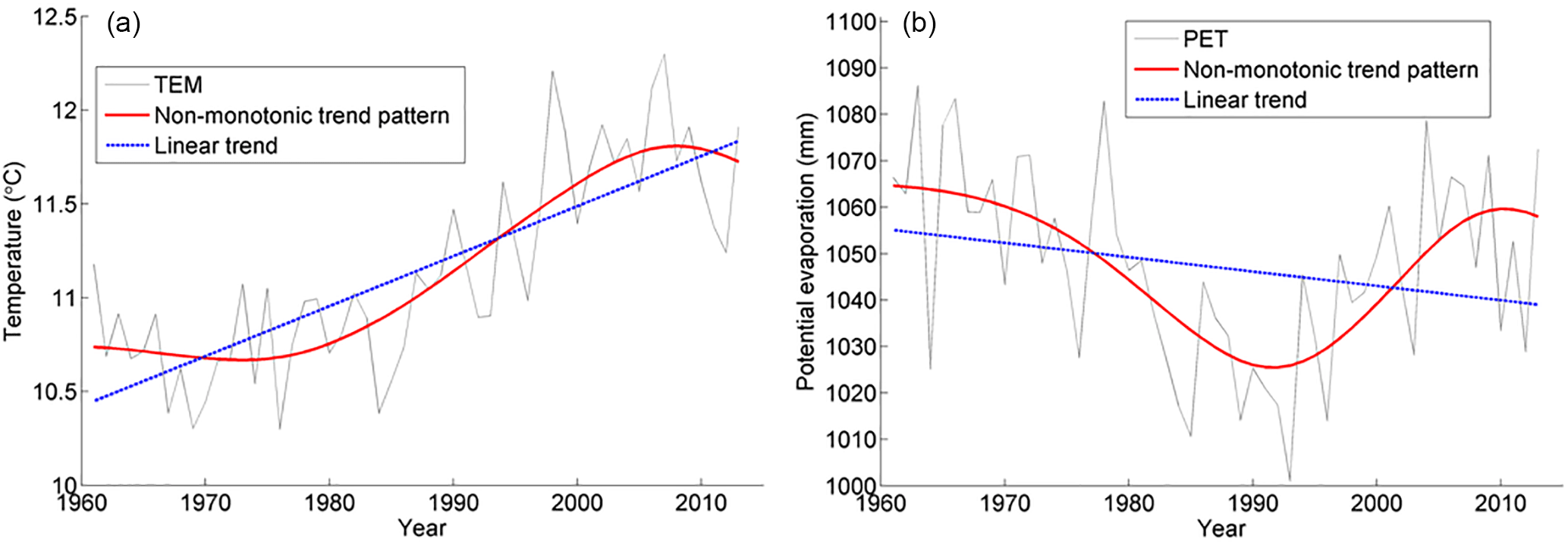
Figure 4Non-monotonic trends in the annual time series of the mean air temperature (TEM, a) and the potential evaporation (PET, b) over China from 1961–2013 identified by the discrete wavelet spectrum (DWS) approach, and the linear trends in the two series.
In the DWS results in Fig. 3, the significance levels of non-monotonic trends did not consistently decrease with data length but showed some fluctuation, as the proportions of different components (including trend) in the original series varied with data length. Furthermore, one would expect that if the trend of a series at a certain length was identified statistically significant, the trend would extend with the increase in data length, thus its significance may be more stable with a larger length of data considered. Using our DWS approach, the trend of series S1 was significant when the data length was larger than 55 (Fig. 3a), being similar to the result of the MK test (Fig. 3c). The trend of the series S2 was statistically significant when the data length was larger than 75 (Fig. 3b). However, using the MK test, the monotonic trend of series S2 was significant only when the data length was between 40 and 185 (Fig. 3d). In summary, the significance of trends identified by our DWS approach was more stable than that detected by the MK test, demonstrating the advantage of the DWS approach in dealing with non-monotonic variations in hydroclimate time series.
3.2 Observed data analysis
We used the annual time series of air temperature (denoted as TEM) and potential evaporation (denoted as PET) over China to further verify the applicability of our developed DWS approach for identifying non-monotonic trends of a time series. These time series were obtained from the hydroclimate data measured at 520 meteorological stations in China, with the same measurement years from 1961 to 2013. The data have been quality checked to ensure their reliability for scientific research. The PET data were calculated from the Penman–Monteith approach (Chen et al., 2005).
The average time series of TEM and PET measured at the 520 stations were first considered. Given the general nonstationary nature of observed hydroclimate time series, linear trends or more generally monotonic curves could not capture the trends with large interdecadal variation and therefore were not particularly physically meaningful. In Fig. 4a, we present the average annual TEM time series visually showing nonstationary characteristics and non-monotonic variation. The TEM series decreased until the 1980s with fluctuations and then sharply rose until the 2000s, followed by a decreasing tendency. The large fluctuation of the average TEM after the late 1990s is the well-known phenomenon of the “global warming hiatus” (Roberts et al., 2015). The linear fitting curve obviously missed out the more complicated trend of the observed temperature time series. Using our DWS approach, we decomposed the TEM series into five (i.e. < log 253) sub-signals using Eqs. (2) and (3), and took the sub-signals under the fifth level as the trend, which realistically presented the nonstationary variability in temperature on long timescales (Fig. 4a).
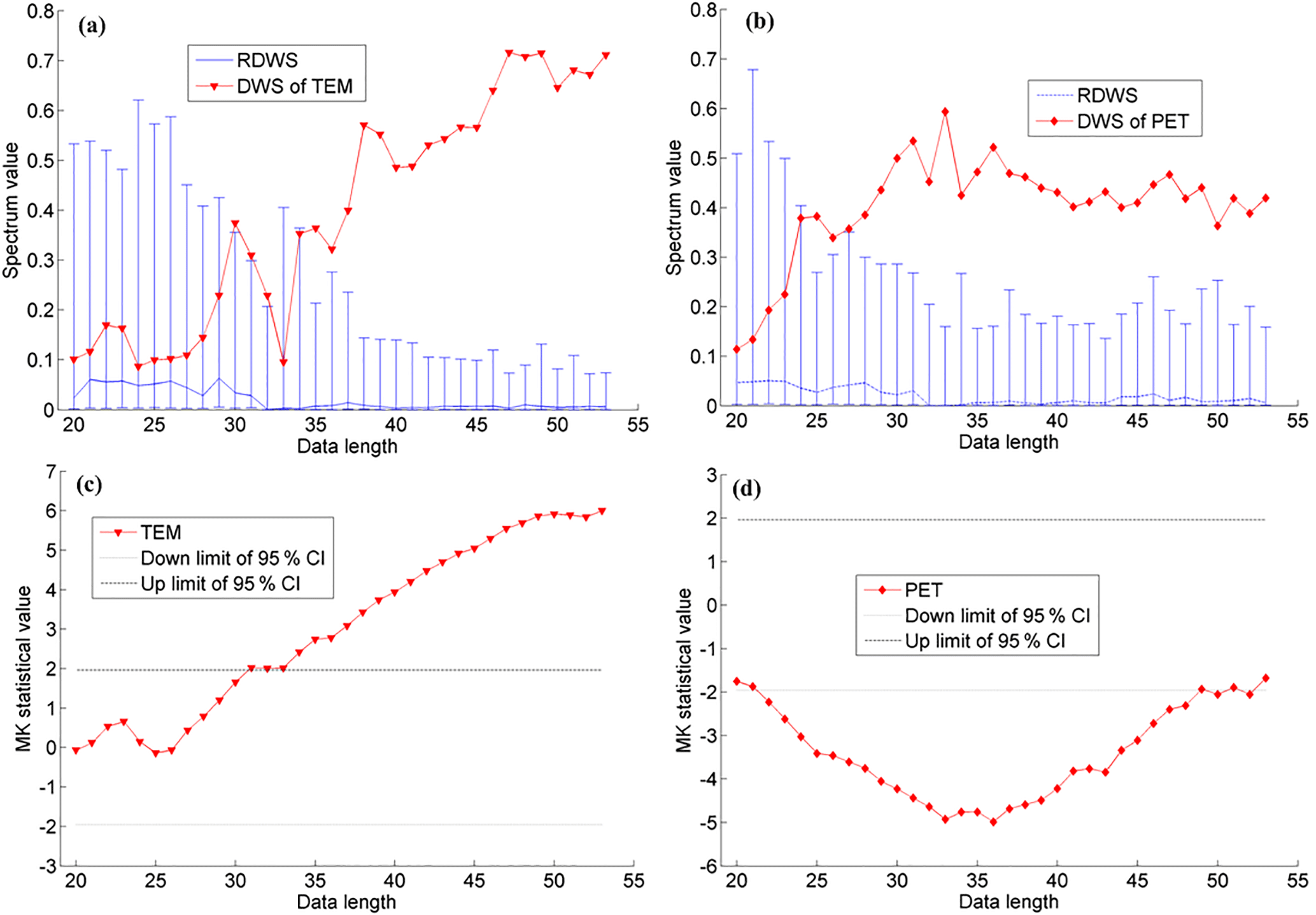
Figure 5Evaluation of statistical significance of non-monotonic trends in the annual time series of the mean air temperature (TEM, a) and the potential evaporation (PET, b) over China with different data length by the discrete wavelet spectrum (DWS) approach, and the results by the Mann–Kendall (MK) test (c, d). In panels (a) and (b), the blue line is the reference discrete wavelet spectrum (RDWS) with 95 % confidence interval under each data length and in panels (c) and (d), the two black horizontal lines indicate the 95 % confidence interval (CI) with the thresholds of ±1.96 in the MK test.
We also applied the DWS approach to the average annual PET time series. In the time series of PET (Fig. 4b), there was a decreasing trend for the period from 1961 to the 1990s, which is the well-known “evaporation paradox” leading to controversial interpretations continuing over the last decade of hydrological cycles (Brutsaert and Parlange, 1998; Roderick and Farquhar, 2002). That decreasing trend was then followed by an abrupt increase around the 1990s, almost the same time when solar radiation was observed to be reversing its trend, widely termed as “global dimming to brightening” (Wild, 2009). Surprisingly, after the mid-2000s, PET started to decrease again (Fig. 4b). Sometimes, one would propose to fit linear curves for separate time periods. Again, linear curves could not capture the overall non-monotonic trend of the PET series. Using the same DWS approach, we identified the non-monotonic trend of the PET time series (Fig. 4b), which captured the two turning points of the changing trends in the 1990s and the 2000s.
The changes in trends in terms of magnitudes and signs for different periods led to the difficulty in assessing and interpreting the significance of trends. For example, the PET time series showed a significant decrease using the MK test (−3.76 < −1.96) during 1961–1992 (Fig. 5d). At that moment before the reversed trend was reported, the significant decrease could be literally interpreted, as that PET had significantly declined and might be declining in the future. However, the PET time series reversed after the 1990s and again in the 2000s, with an insignificant overall trend for the whole period of 1961–2013. For the more or less monotonic time series of the TEM series (1961–2013), the MK test detected a significant increase (6.00 > 1.96; Fig. 5c), which led to the surprise when TEM was reported to have stopped increasing after the late 1990s. In summary, it becomes vital to develop an approach for testing the significance of trend, which is suitable for non-monotonic time series as this is an important basis and a prerequisite for hydrological simulation and prediction on decadal scales.
In this study, building on the DWT, we proposed an operational approach, i.e. DWS, for evaluating the significance of non-monotonic trends in TEM (Fig. 5a) and PET (Fig. 5b) series. For comparison purposes, we also conducted the significance test for the two time series using the MK test (Fig. 5c and d). Similar to Fig. 3, we changed the data length to investigate the stability of statistical significance (Fig. 5). Again, results indicated that the 95 % confidence interval for evaluating the statistical significance of non-monotonic trend generally decreased with data length, which was different from the constant thresholds of ±1.96 adopted in the MK test. The significance test using our DWS approach appeared to be more stable with data length than the MK test (Fig. 5). Using our DWS approach, the trend in the TEM series became significant when the data length increased to 30, and the significance was more stable when it was greater than 35 (Fig. 5a). For the case of the PET series, the trend became statistically significant when the data length was larger than 25 (Fig. 5b). The findings here have important implications for non-monotonic hydroclimate time series analysis, in that the timescale of defining climate and climate change by the World Meteorological Organization is usually 30 years (Arguez and Vose, 2011) and in hydrological practice it is between 25–30 years.
For the whole time series investigated here, whose length was larger than 30 years, we were able to examine the significance using the developed DWS approach. Combining the trend in Fig. 4a and the significance test in Fig. 5a, we confirmed that the trend of the TEM time series from 1961–2013 identified in this study was significant at 95 % confidence interval. Similarly, the trend in PET was also significant (Figs. 4b and 5b). The significance test results suggested that the three main stages of the series (red lines; Fig. 4) were detectable as the overall trend from the variability of the series and were vital to understanding how the TEM and the PET series were changing on interdecadal scales. In particular, the reversed change in PET and its significance can be revealed by our DWS approach, which can provide more useful and physically meaningful information.
We further detected and evaluated the significance of non-monotonic trends of the PET time series measured at 520 stations for investigating their spatial difference. Because the trends in the annual TEM time series were quasi-monotonic, and they were statistically significant at most of the stations (whether using our DWS approach or the MK test), further details of TEM data were not repeated here. As for the trends in the PET data, the results obtained from our DWS approach (Fig. 6b) and those in the MK test (Fig. 6a) presented substantial differences. When conducting the MK statistical significance test, the monotonic trends were detected as significant in the annual PET time series measured at the 230 stations. Significant downward monotonic trends were mainly found in the southern part of the Songliao River basin, the Hai River basin, the Huai River basin, some regions in south China, and northwest China. Significant upward monotonic trends were mainly found in the northern part of the Songliao River basin, the upper reach of the Yellow River basin, the southwest corner of China, and some regions in the Yangtze River Delta.
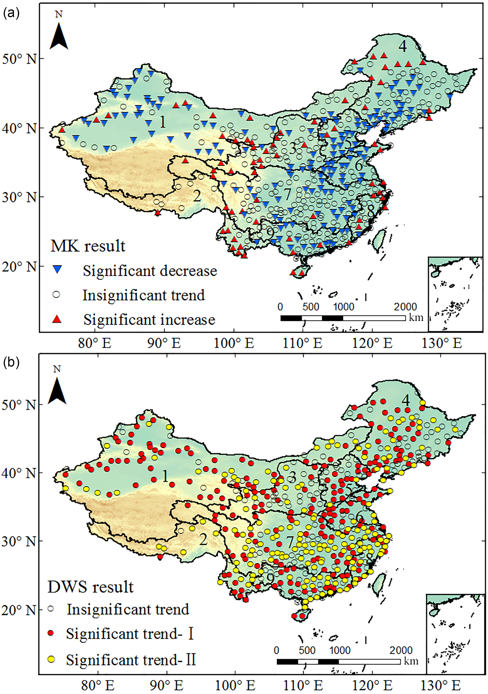
Figure 6Spatial distribution of the significance of trends in the annual potential evaporation data during 1961–2013 and measured at 520 weather stations over China. The result (a) was obtained from the Mann–Kendall (MK) test. The result (b) was obtained from the developed discrete wavelet spectrum (DWS) approach, in which significant trend-I means those significant trends (at 230 stations) can be identified by both the DWS approach and the MK test, but significant trend-II means those significant trends (at 150 stations) can only be identified by the DWS approach but not the MK test. The labels on the map correspond to the following: 1, the northwest inland river basin; 2, the southwest river basin; 3, the Yellow River basin; 4, the Songliao River basin; 5, the Haihe River basin; 6, the Huaihe River basin; 7, the Yangtze River basin; 8, the southeast river basin; and 9, the Pearl River basin.
Comparatively, significant non-monotonic trends in the PET time series were detected at 380 stations throughout China. That means that those annual PET time series measured at 150 stations (28.8 % of the total stations and mainly in the southern part of China) mainly indicated non-monotonic variations rather than monotonic trends on interdecadal scales, with similar phenomena as shown in Fig. 4b, and their significance was underestimated by the MK test, which can only handle monotonic trends. Previous studies (Zhang et al., 2016; Jiang et al., 2007) indicated that potential evaporation was influenced by more physical factors (precipitation, air temperature, wind speed, relative humidity, etc.) in the southern part of China rather than the northern part; thus, the potential evaporation process in south China presented a more complex variability and was more difficult to detect and attribute its physical causes. As a result, it is known here that the annual potential evaporation process in most parts of China indicated significance variability on interdecadal scales, but it was underestimated by the conventional MK test; moreover, only considering monotonic trends would cause a great difficulty in accurately understanding the temporal and spatial variability in potential evaporation and the hydroclimate process in China, and would also be unfavourable for hydrological predictions on interdecadal scales. Our results suggest that the non-monotonic trend of hydroclimate time series and its significance should be carefully identified and evaluated.
Climate and hydrological processes are changing non-monotonically. Identification of linear (or monotonic) trends in hydroclimate time series, as a common practice, cannot capture the detail of the non-monotonic trend in the time series on long timescales, and this can lead to misinterpreting climatic and hydrological changes. Therefore, revealing the trend of the time series and assessing its significance from the usually varying hydroclimate process remains a challenge. To that end, we developed the DWS approach for identifying the non-monotonic trend in hydroclimate time series, in which the DWT is used first to separate the trend, and its statistical significance is then evaluated by using the discrete wavelet spectrum (Fig. 1). Using two typical synthetic time series, we examined the developed DWS approach and find that it can precisely identify non-monotonic trends in the synthetic time series (Fig. 2) and has an advantage in significance testing (Fig. 3).
Using our DWS approach, we identify the trend in the annual time series of average temperature and potential evaporation over China from 1961–2013 (Fig. 4). The identified non-monotonic trends precisely describe how TEM and PET are changing on interdecadal timescales. Of particular interest here is that the DWS approach can help detect both the “warming” and the “warming hiatus” in the temperature time series, and reveal the reversed changes and the latest decrease in the PET time series. The DWS approach can provide other aspects on the trends in the time series, i.e. the significance test. Results show that the trends become more significant and the significance test becomes more stable when the time series is longer than a certain period like 30 years or so, the widely defined “climate” timescale (Fig. 5). Using the DWS approach, in both time series of mean air temperature and potential evaporation, the identified trends are found to be significant (Fig. 5). Moreover, the significance of trends in the PET time series obtained from the DWS approach and the MK test obviously has different spatial distributions (Fig. 6). The variability in the hydroclimate process on long timescales, especially for non-monotonic trends, would be underestimated by the MK test, which causes a great difficulty in understanding and interpreting the spatiotemporal variability in hydroclimate processes. Comparatively, the developed DWS approach can quantitatively assess the statistical significance of non-monotonic trends in the hydroclimate process, and so can meet practical needs much better.
In summary, our results suggest that the non-monotonic trends of hydroclimate time series and its statistical significance should be carefully identified and evaluated, and the DWS approach developed in this study has the potential for wider use in the hydrological and climate sciences.
The observed TEM data (Dataset of Daily Climate Data from Chinese Surface Stations, V3.0) used in the study were obtained from the China Meteorological Data Sharing Service Center (http://data.cma.cn/). The synthetic time series and the computed PET data used in this study are available from the authors upon request (sangyf@igsnrr.ac.cn).
The authors declare that they have no conflict of interest.
The authors gratefully acknowledged the valuable comments and suggestions
given by Stacey Archfield and the anonymous
reviewers. This study was financially supported by the National Natural
Science Foundation of China (nos. 91647110, 91547205, 51579181), the Program
for the “Bingwei” Excellent Talents from the Institute of Geographic
Sciences and Natural Resources Research, CAS, the Youth Innovation Promotion
Association CAS (no. 2017074), the Open Foundation of State Key
Laboratory of Hydrology-Water Resources and Hydraulic Engineering
(no. 2015491811), and the National Mountain Flood Disaster Investigation
Project (no. SHZH-IWHR-57).
Edited by: Stacey Archfield
Reviewed by: three anonymous referees
Adam, J. C. and Lettenmaier, D. P.: Application of new precipitation and reconstructed streamflow products to streamflow trend attribution in northern Eurasia, J. Climate, 21, 1807–1828, 2008.
Allen, M. R. and Ingram, W. J.: Constraints on future changes in climate and the hydrologic cycle, Nature, 419, 224–232, 2002.
Almasri, A., Locking, H., and Shukar, G.: Testing for climate warming in Sweden during 1850–1999 using wavelet analysis, J. Appl. Stat., 35, 431–443, 2008.
Arguez, A. and Vose, R. S.: The definition of the standard WMO climate normal: The key to deriving alternative climate normal, B. Am. Meteorol. Soc., 92, 699–704, 2011.
Brutsaert, W. and Parlange, M. B.: Hydrologic cycle explains the evaporation paradox, Nature, 396, 30, https://doi.org/10.1038/23845, 1998.
Burn, D. H. and Hag Elnur, M. A.: Detection of hydrologic trends and variability, J. Hydrol., 255, 107–122, 2002.
Chen, D., Gao, G., Xu, C. Y., Guo, J., and Ren G.: Comparison of the Thornthwaite method and pan data with the standard Penman-Monteith estimates of reference evapotranspiration in China, Clim. Res., 28, 123–132, 2005.
Cohn, T. A. and Lins, H. F.: Nature's style: naturally trendy, Geophys. Res. Lett., 32, L23402, https://doi.org/10.1029/2005GL024476, 2005.
de Artigas, M., Elias, A., and de Campra, P.: Discrete wavelet analysis to assess long-term trends in geomagnetic activity, Phys. Chem. Earth, 31, 77–80, 2006.
Diffenbaugh, N. S., Giorgi, F., and Pal, J. S.: Climate change hotspots in the United States, Geophys. Res. Lett., 35, L16709, https://doi.org/10.1029/2008GL035075, 2008.
Dixon, H., Lawler, D. M., and Shamseldin, A. Y.: Streamflow trends in western Britain, Geophys. Res. Lett., 32, L19406, https://doi.org/10.1029/2006GL027325, 2006.
Foufoula-Georgiou, E. and Kumar, P. (Eds.): Wavelets in geophysics, vol. 4, Academic Press, San Diego, USA, 2014.
Gaucherel, C.: Use of wavelet transform for temporal characteristics of remote watersheds, J. Hydrol., 269, 101–121, 2002.
Gong, S. L., Zhao, T. L., Sharma, S., Toom-Sauntry, D., Lavoue, D., Zhang, X. B., Leaitch, W. R., and Barrie, A.: Identification of trends and interannual variability of sulfate and black carbon in the Canadian High Arctic: 1981–2007, J. Geophys. Res.-Atmos., 115, D07305, https://doi.org/10.1029/2009JD012943, 2010.
Jiang, T., Chen, Y. D., Xu, C. Y., Chen, X., Chen, X., and Singh, V. P.: Comparison of hydrological impacts of climate change simulated by six hydrological models in the Dongjiang Basin, South China, J. Hydrol., 336, 316–333, 2007.
Kallache, M., Rust, H. W., and Kropp, J.: Trend assessment: applications for hydrology and climate research, Nonlin. Processes Geophys., 12, 201–210, https://doi.org/10.5194/npg-12-201-2005, 2005.
Kosaka, Y. and Xie, S. P.: Recent global-warming hiatus tied to equatorial Pacific surface cooling, Nature, 501, 403–407, 2013.
Labat, D.: Recent advances in wavelet analyses: Part 1. A review of concepts, J. Hydrol., 314, 275–288, 2005.
Labat, D., Ababou, R., and Mangin, A.: Rainfall-runoff relations for karstic springs. Part II: continuous wavelet and discrete orthogonal multiresolution analyses, J. Hydrol., 238, 149–178, 2000.
Medhaug, I., Stolpe, M. B., Fischer, E. M., and Knutti, R.: Reconciling controversies about the “global warming hiatus”, Nature, 545, 41–47, 2017.
Milly, P. C. D., Betancourt, J., Falkenmark, M., Hirsch, R. M., Kundzewicz, Z. W., Lettenmaier, D. P., and Stouffer, R. J.: Stationarity is dead: whither water management?, Science, 319, 573–574, 2008.
Nalley, D., Adamowski, J., and Khalil, B.: Using discrete wavelet transforms to analyze trends in streamflow and precipitation in Quebec and Ontario (1954–2008), J. Hydrol., 475, 204–228, 2012.
Nourani, V., Baghanam, A. H., Adamowski, J., and Kisi, O.: Applications of hybrid wavelet-artificial Intelligence models in hydrology: A review, J. Hydrol., 514, 358–377, 2014.
Partal, T. and Cigizoglu, H. K.: Estimation and forecasting of daily suspended sediment data using wavelet-neural networks, J. Hydrol., 358, 317–331, 2008.
Partal, T. and Kucuk, M.: Long term trend analysis using discrete wavelet components of annual precipitation measurements in Marmara region (Turkey), Phys. Chem. Earth, 31, 1189–1200, 2006.
Percival, D. B. and Walden, A. T.: Wavelet Methods for Time Series Analysis, Cambridge University Press, Cambridge, UK, 2000.
Rajaram, H., Bahr, J. M., Blöschl, G., Cai, J. X., Scott Mackay, D., Michalak, A. M., Montanari, A., Sanchez-Villa, X., and Sander, G.: A reflection on the first 50 years of Water Resources Research, Water Resour. Res., 51, 7829–7837, 2015.
Roberts, C. D., Palmer, M. D., McNeall, D., and Collins, M.: Quantifying the likelihood of a continued hiatus in global warming, Nat. Clim. Change, 5, 337–342, 2015.
Roderick, M. L. and Farquhar, G. D.: The cause of decreased pan evaporation over the past 50 years, Science, 298, 1410–1411, 2002.
Sang, Y. F.: A practical guide to discrete wavelet decomposition of hydrologic time series, Water Resour. Manag., 26, 3345–3365, 2012.
Sang, Y. F., Wang, Z., and Liu, C.: Period identification in hydrologic time series using empirical mode decomposition and maximum entropy spectral analysis, J. Hydrol., 424, 154–164, 2012.
Sang, Y. F., Wang, Z., and Liu, C.: Discrete wavelet-based trend identification in hydrologic time series, Hydrol. Process., 27, 2021–2031, 2013.
Stocker, T. F., Qin, D., Plattner, G. K., Tignor, M., Allen, S. K., Boschung, J., Nauels, A., Xia, Y., Bex, B., and Midgley, B. M.: IPCC: Climate Change 2013: The Physical Science Basis, Contribution of Working Group I to the Fifth Assessment Report of the Intergovernmental Panel on Climate Change, Cambridge Univ. Press, Cambridge, UK, 2013.
Torrence, C. and Compo, G. P.: A practical guide to wavelet analysis, B. Am. Meteorol. Soc., 79, 61–78, 1998.
Trenberth, K. E., Dai, A., der Schrier, G., Jones, P. D., Barichivich, J., Briffa, K. R., and Sheffield, J.: Global warming and changes in drought, Nat. Clim. Change, 4, 17–22, 2014.
Wild, M.: Global dimming and brightening: A review, J. Geophys. Res., 114, D00D16, https://doi.org/10.1029/2008JD011470, 2009.
Yue, S., Pilon, P., and Cavadias, G.: Power of the Mann-Kendall and Spearman's rho tests for detecting monotonic trends in hydrological series, J. Hydrol., 259, 254–271, 2002.
Zhang, J., Sun, F., Xu, J., Chen, Y., Sang, Y. F., and Liu, C.: Dependence of trends in and sensitivity of drought over China (1961–2013) on potential evaporation model, Geophys. Res. Lett., 43, 206–213, 2016.