the Creative Commons Attribution 4.0 License.
the Creative Commons Attribution 4.0 License.
 | 01 Mar 2019
Dew frequency across the US from a network of in situ radiometers
François Ritter
Max Berkelhammer
Daniel Beysens
Dew formation is a ubiquitous process, but its importance to energy budgets or ecosystem health is difficult to constrain. This uncertainty arises largely because of a lack of continuous quantitative measurements on dew across ecosystems with varying climate states and surface characteristics. This study analyzes dew frequency from the National Ecological Observatory Network (NEON), which includes 11 grasslands and 19 forest sites from 2015 to 2017. Dew formation is determined at 30 min intervals using in situ radiometric surface temperatures from multiple heights within the canopy along with meteorological measurements. Dew frequency in the grasslands ranges from 15 % to 95 % of the nights with a strong linear dependency on the nighttime relative humidity (RH), while dew frequency in the forests is less frequent and more homogeneous (25±14 %, 1 standard deviation – SD). Dew mostly forms at the top of the canopy for the grasslands due to more effective radiative cooling and within the canopy for the forests because of higher within the canopy RH. The high temporal resolution of our data showed that dew duration reaches maximum values (∼6–15 h) for RH∼96 % and for a wind speed of , independent of the ecosystem type. While dew duration can be inferred from the observations, dew yield needs to be estimated based on the Monin–Obukhov similarity theory. We find yields of (1 SD from nine grasslands) similar to previous studies, and dew yield and duration are related by a quadratic relationship. The latent heat flux released by dew formation is estimated to be non-negligible (), associated with a Bowen ratio of ∼3. The radiometers used here provide canopy-averaged surface temperatures, which may underestimate dew frequency because of localized cold points in the canopy that fall below the dew point. A statistical model is used to test this effect and shows that dew frequency can increase by an additional ∼5 % for both ecosystems by considering a reasonable distribution around the mean canopy temperature. The mean dew duration is almost unaffected by this sensitivity analysis. In situ radiometric surface temperatures provide a continuous, non-invasive and robust tool for studying dew frequency and duration on a fine temporal scale.


Natural ecosystems are expected to experience more water stress due to a shift in the frequency, intensity and duration of droughts in the context of climate change (Dai, 2013). Second-order processes in the water cycle such as fog deposition (Dawson, 1998), water vapor adsorption (Kosmas et al., 1998) or dew formation (Monteith, 1957) may alleviate or exacerbate water stress on ecosystems, depending on how the frequency of these events changes with rising temperatures. These processes can have a direct impact on the water balance of an ecosystem via the Foliar water uptake mechanism, which allows some plant species to rehydrate themselves by absorbing the residual water on their leaves (Boucher et al., 1995; Munne-Bosch et al., 1999; Burgess and Dawson, 2004). In the example of a redwood forest in California, 80 % of the dominant species have been proven to possess this trait, and it contributed to an increase up to 11 % in their leaf water content (Limm et al., 2009). The impact on the water balance can also be indirect via transpiration suppression (Tolk et al., 1995), with a potential dew-induced decrease of 30 % in transpiration rate (estimated from isotopic methods; Gerlein-Safdi et al., 2018a) or an impressive 100 % increase in the water use efficiency between the dew-affected and the no-dew populations in a semi-arid area (using a photosynthesis and transpiration rate monitor; Ben-Asher et al., 2010). The energy budget of the ecosystem will be affected as well, not only because of a change in the sensible and latent heat fluxes but also in the emissivity of the surface. An increase of 10 % in the surface albedo due to the presence of dew has been reported from an analysis using satellite data (Minnis et al., 1997). All these combined effects on the water and energy balance might enable animal and plant species to survive longer droughts in the future; see Wang et al. (2017b) for a review on the ecological significance of non-rainfall water inputs.
Dew formation is the water vapor condensation on a surface when the surface temperature drops below the dew point temperature of the air. It occurs almost exclusively at night when reduced input of shortwave radiation generates a negative net radiation balance at the surface. Based on a recent review (Tomaszkiewicz et al., 2015) that includes 25 studies using dew condensers, a typical dew frequency is 41±14 % of the nights (1 standard deviation or SD), and a typical dew yield is (1 SD), in an average study period of 1 year. Dew formation is known to be abundant even in semi-arid areas that are in close proximity to a moisture source. For example, dew occurred during 78 % of the nights during a 4-year period in a semi-arid coastal steppe (Uclés et al., 2014) and 77 % of the nights during the growing season at the edge of a desert oasis (Zhuang and Zhao, 2017). The three most important limitations of dew formation are relative humidity, the efficiency of radiative cooling (driven by cloud cover, biomass density, and vapor pressure of air and surface emissivity) and surface wind speed (influenced by regional climate, local topography and canopy structure). The relative humidity is directly related to the dew point temperature of the air, while the radiative cooling creates a difference in temperature between the surface of the canopy and the air at night. Lastly, the wind speed increases the heat exchange between the cold surface and the air, thus lowering the available energy for condensation and eventually reducing the dew yield. It is also important to note that the two extreme cases where the relative humidity is at 100 % or the wind speed is close to 0 m s−1 are not beneficial for dew formation either. The radiative cooling is lowered or even canceled in the first case (“radiative fog”), and in the second case, some convection is needed to replenish the available water vapor in the boundary layer of the canopy. Dew formation is therefore a subtle process that requires an adequate balance between relative humidity, radiative cooling and wind speed.
So far, no unique standardized method currently exists to measure dew formation. The previously mentioned radiative passive condenser (RDC) is usually a flat tilted plate (area of ∼1 m2), thermally isolated from the ground, from which dew droplets are collected under gravity flow (Maestre-Valero et al., 2015). It is also possible to weigh materials (tissues, woods and plastic) before and after the dew event to calculate the dew yield (Pan et al., 2010) or to use leaf wetness sensors to estimate the presence or absence of wetness on its surface (Moro et al., 2009; Berkelhammer et al., 2013). These approaches provide a potential dew frequency and yield, but the artificial surfaces used to collect dew droplets are not representative of the ecosystem in terms of thermal and radiative properties like the conductivity or emissivity (Sentelhas et al., 2004; Maestre-Valero et al., 2011). Additionally, natural ecosystems are dynamic environments that vary seasonally and grow or decline over decades. Long-term dew formation measurements therefore need to capture this evolution in the canopy. For example, an approach that is more ecosystem-focused takes advantage of large lysimeters to weigh dew formation at night on natural ecosystems (Meissner et al., 2007). In a study using two high precision lysimeters on temperate grasslands for 2 years, Xiao et al. (2009) shows that the maximum nighttime dew yield is limited by the growth of the canopy height for a maize plantation, from 0.1 mm night−1 (canopy height below 0.2 m) to 0.5 mm night−1 (same site, but canopy height at 2 m). This result is obviously influenced by the meteorological conditions associated with the growing season, but it also shows the importance of the canopy structure to the dew frequency and yield. To summarize, although extensive work has been done to measure dew formation there remains a lack of data using continuous measurements performed in different ecosystems with the same standardization. The measurement approach either uses a surface that is not representative of the properties and dynamic of the canopy (RDC, leaf wetness sensors, etc.) or generates a highly local measurement (lysimeters). It is therefore difficult to establish a global or continental network of standardized dew measurements over a sufficiently long period of time to analyze the impact of climate change on dew frequency, duration and yield. Such data are needed to validate dew models, which provide a tool for testing the sensitivity of dew formation to different forcing mechanisms.
Models of dew formation are usually designed from an energy balance, like the Penman–Monteith equation (Monteith et al., 1965), where the latent heat released by condensation is the parameter to solve for. Otherwise, semi-empirical models are also reliable and are calculated from the relationships between dew formation and its drivers: relative humidity, wind speed and cloud cover (Beysens, 2016). These models are fed with classical meteorological measurements, and they have been reasonably well validated with direct dew measurements. For example, in Beysens (2016), the average slope between the cumulated experimental yield and the cumulated predicted yield is 0.8±0.2 (1 SD) based on 10 studies using RDCs. Models give the opportunity to study dew formation on a larger scale, but only two recent attempts have been published: a global dew yield estimation based on reanalysis data (Vuollekoski et al., 2015) and a map of the dew yield on the Mediterranean coast based on data from a network of traditional weather stations (Tomaszkiewicz et al., 2016). These studies estimate dew yield using semi-empirical models, which consider the surface receiving dew formation to be a flat plate to simplify the equations of heat and vapor transfer. Both methods detect a significant change in the dew yield over a climatic timescale, for example ±10 % change from 1979 to 2012 in different parts of the world (Vuollekoski et al., 2015) or a 27 % decrease in future summers in the Mediterranean Basin from 2013 to 2080 (Tomaszkiewicz et al., 2016). However, these attempts did not have access to the surface temperature of the canopy and had to implicitly retrieve it from an energy balance or assume it is close to the dew point temperature. This problem is the same encountered for energy balance models, for example Richards (2009), Maestre-Valero et al. (2012) or Gerlein-Safdi et al. (2018b). It is well known in the eddy-covariance field that the energy balance closure is less reliable at night simply because of the higher uncertainties in the latent and sensible fluxes associated with a decrease in temperature and wind speed after sunset (de Roode et al., 2010). Indeed, as the atmospheric stability increases at night, the turbulent component of the energy transfer decreases relative to the radiative component. The surface temperature retrieval is therefore associated with a high uncertainty, as it depends on the net radiation, the ground flux (driven by the soil temperature gradient), the wind speed, the air temperature, and the exchange of latent heat from condensation or possible nocturnal evapotranspiration. This problem can be bypassed by estimating the surface temperature using in situ radiometric surface temperature measurements of different canopies and then simply comparing them with the dew point temperatures of the air.
The scientific literature about infrared thermal radiometers (or IR radiometers) is abundant in the remote sensing field (see Kalma et al., 2008, for a review) because satellites offer the opportunity to estimate the sea or land surface temperature on a global scale. However, in situ radiometric measurements of the surface temperature in natural ecosystems are less well documented (Stewart et al., 1994; Troufleau et al., 1997; Suleiman and Crago, 2004; Payero and Irmak, 2006; Sánchez et al., 2008, 2011, 2014). Studies of the nighttime surface temperatures using this approach are even more limited (Bosveld et al., 1999; Jacobs et al., 2006; Maestre-Valero et al., 2015) due to the overall lack of interest in the nocturnal processes when the latent or sensible heat is low and there is no photosynthetic activity. The surface temperature is retrieved from the infrared emissions using the Stefan–Boltzmann law and is then usually corrected with respect to the surface emissivity. For the new generation of IR radiometers (Apogee SI-111, used in this study), the order of magnitude of the uncertainty is (Payero and Irmak, 2006), associated with a response time of 0.6 s. Two studies have validated the use of in situ IR radiometers and dew point temperature to predict the absence or presence of dew formation by comparison with the RDC and leaf wetness sensor data (Maestre-Valero et al., 2015) or lysimeter data (Jacobs et al., 2006). The IR radiometers are therefore suitable for studying dew frequency and dew duration. However, the dew yield is a parameter that is more difficult to constrain because it requires an estimate of the aerodynamic resistance between the leaf surface and the air for vapor transfer, which depends on the wind speed, canopy structure and atmospheric stability.
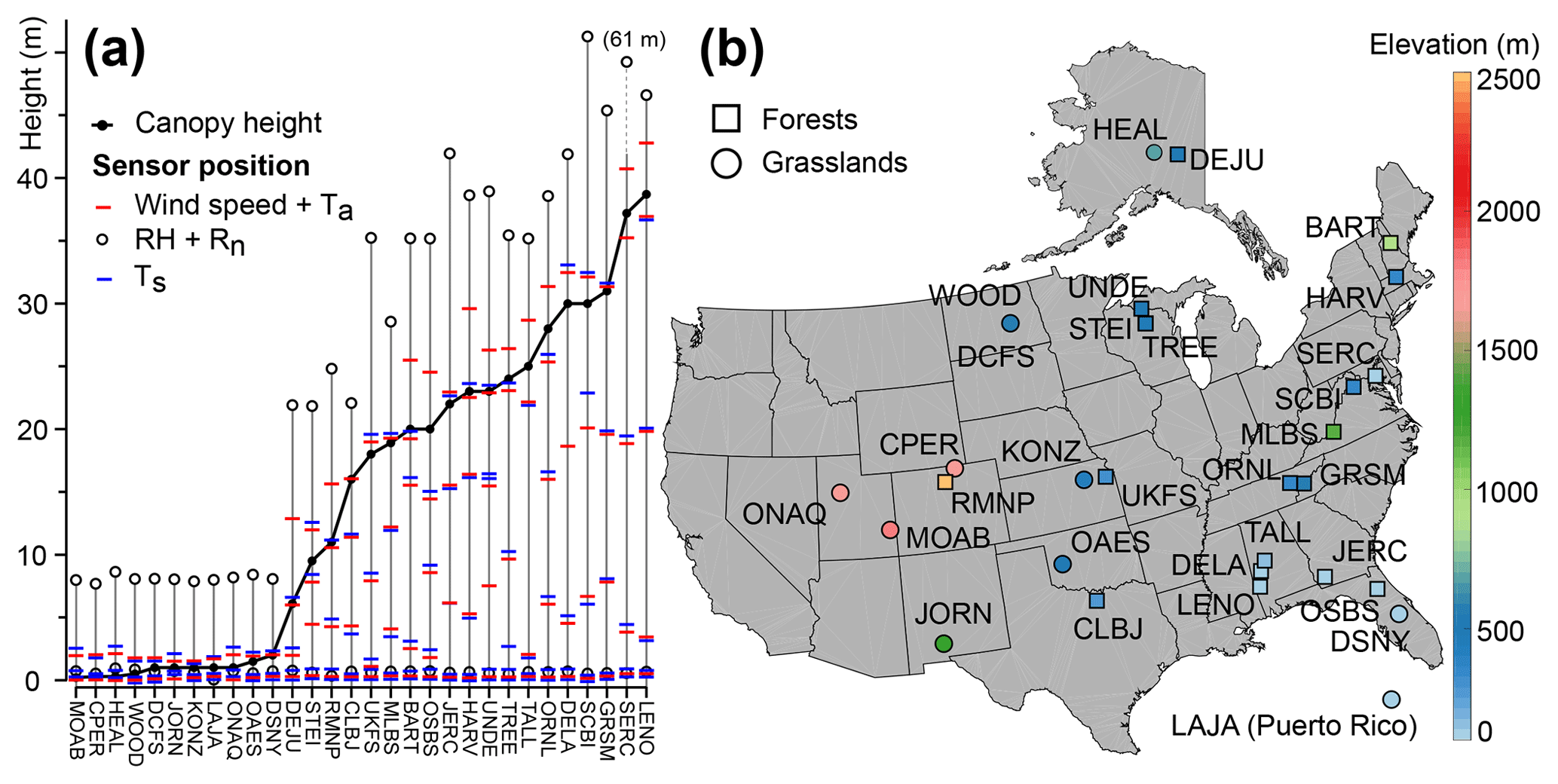
Figure 1(a) Vertical position of the sensors for each site (ordered with an increasing canopy height). (b) Elevation and locality of the sites in the USA.
IR radiometers are a standard component of the National Ecological Observatory Network (NEON), which was established in 2012 to assess the change of ecosystems on a continental scale over 30 years. NEON recently released preliminary data that includes traditional meteorological measurements and radiometric temperature of the canopy of 11 grasslands (2748 nights) and 19 forests (4747 nights) in the USA with a 30 min resolution from 2015 to 2017 (Fig. 1). This network has the advantage of providing a measurement that is continuous, captures an average condition for the whole canopy of diverse ecosystems, and neither relies on artificial surfaces nor requires solving the energy balance for canopy or soil surfaces at night. We focus in this paper on the growing season when temperatures are above 0 ∘C (frost events are therefore excluded). We analyze the vertical variability of the relative humidity and surface temperature associated with each site at night (Fig. 2); show how the nighttime radiative cooling is limited by the relative humidity and drives the difference in temperature between the air and the surface (Fig. 3); present the dew frequency, duration and yield in forest and grassland ecosystems across very different climatic conditions (Figs. 4 and 5); estimate and compare the sensible, latent and radiative flux associated with a dew event (Fig. 6); constrain the sensitivity of dew duration to relative humidity (Fig. 7) and wind speed (Fig. 8); describe the nocturnal cycles associated with the absence or presence of dew formation (Figs. 9 and 10); and finally interrogate the possible importance of the spatial variability of the surface temperature on the dew frequency using a Monte Carlo sensitivity analysis (Fig. 11).
Table 1Summary of the results for the grassland sites ordered with an increasing RH. Dew frequency, duration, yield and meteorological parameters (averaged from 23:00 to 05:00 the next day) have been calculated at the top of the canopy, except RH (close to the ground). C.h. stands for canopy height, and elev. stands for elevation.
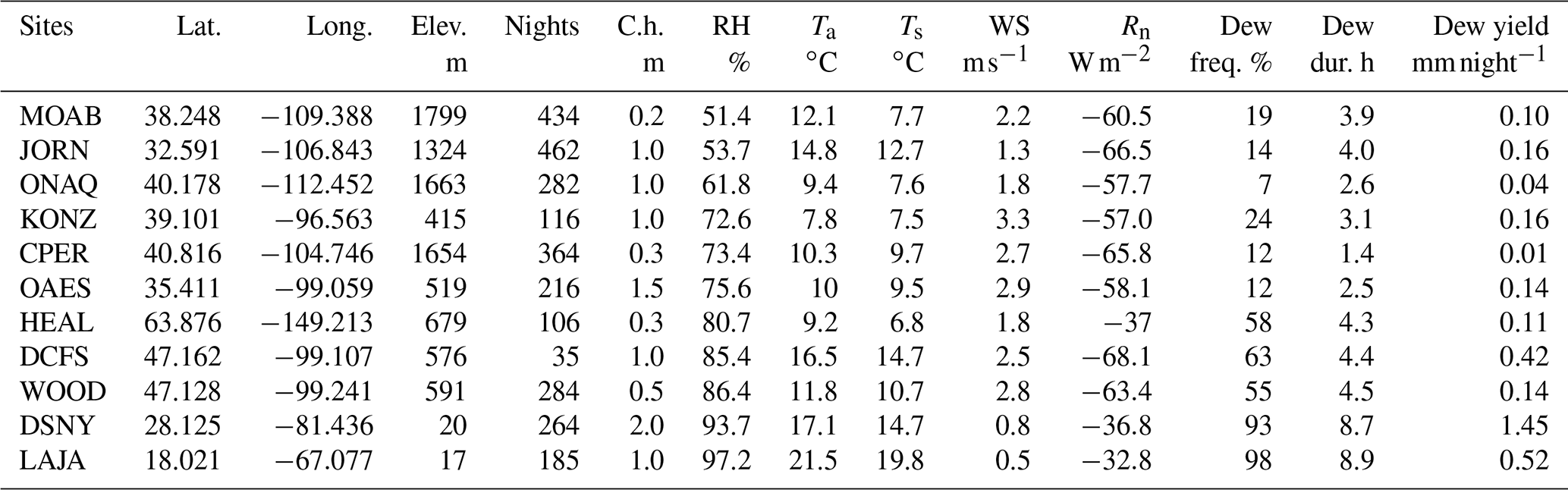
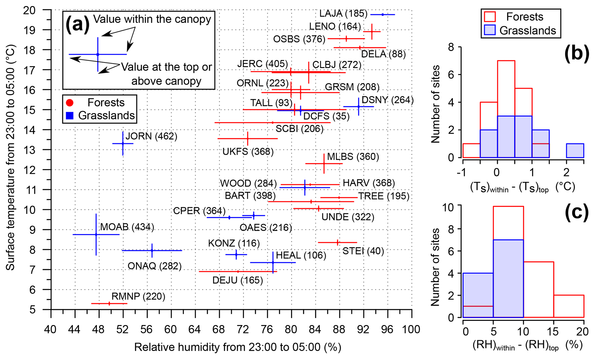
Figure 2(a) Ts versus RH from 23:00 to 05:00 the next day over the growing season for each site (number of nights is indicated in parenthesis). Four mean values have been calculated per site, two from the sensors within canopy and two from the sensors at the top of canopy. (b, c) Histograms of the difference in Ts (and RH) between that within canopy and that at the top of the canopy. SERC is missing because of a sensor failure above canopy.
Description of the data. All the analyses performed in this study are based on the preliminary dataset recently released by NEON with a 30 min resolution from 2015 to 2017 (downloaded from http://data.neonscience.org, last access: 10 April 2018). Meteorological parameters were measured at different heights from a tower (Fig. 1), and we focused on 11 grasslands (2748 nights) and 19 forests (4747 nights) with the following measurements available from 16:00 to 10:00 the next day (local time used in this paper): radiometric surface temperature (Ts; Apogee SI-111), relative humidity (RH; Vaisala HMP155), pressure (P; Vaisala PTB330), air temperature (Ta; Met One Instruments 62789 Aspirated Radiation Shield), wind speed (WS; Gill's WindObserver II 2-D Sonic Anemometer) and net radiation above the canopy (Rn; NR01 net radiation sensor). The code name, sample size, elevation, location and canopy height of each site are reported in Tables 1 and 2. For each data point, NEON provides an expanded uncertainty that includes calibration, a data acquisition system and natural variance. These expanded uncertainties are dynamically calculated and therefore take into account possible sensor drifts between calibrations. Typical nighttime values of these expanded uncertainties are for Ts, ±2.2 % for RH, for WS, for Ta and for Rn. These 30 min uncertainties will be considerably reduced by the calculation of mean values on a nightly timescale and then over the full period of study (∼250 nights per site on average) so that the cumulative uncertainties become negligible with a sample size this large. For example for only one night (from 23:00 to 05:00 the next day), the standard error of the mean value of Ts and RH is 0.2 ∘C and 0.6 % (respectively). A Monte Carlo simulation is run to quantify the sensitivity of the dew frequency to the variability of the surface temperature (see details below).
Division of the canopy. The data were separated into two layers of vegetation: “within the canopy” (spatial average of the wind speed, air and surface temperature measurements below the top of the canopy) and “at the top of the canopy” (using the IR radiometer, with air and wind speed sensors closest to the top of the canopy). For the grasslands, the RH sensor close to the ground is used for both layers because the other sensor is significantly above the top of the canopy (∼8 m; see Fig. 1). For the forests, the RH sensor close to the ground is used for the layer within the canopy, and the RH sensor above the canopy is used for the layer at the top of the canopy. Although vertical interpolation could have been used to estimate RH co-located with the radiometric surface temperature measurement, this would have been inappropriate here because the canopy structure or atmospheric stability does affect the vertical profile of RH. Finally, a dew point temperature (Td) is calculated for both layers following the equation in Wagner and Pruß (2002) and using the respective Ta and RH of each layer.
IR radiometer information. The IR radiometer used by NEON is the Apogee SI-111, with a response time of 0.6 s. The spectral range is 8 to 14 µm (atmospheric window), and the IR radiometer is fully operational at RH=100 %. The height of the sensors depends on the site (see Ts in Fig. 1), and their pointing angle is usually 22∘ from vertical. NEON applies a correction for temperature of the sensor, however the radiometric measurements are not corrected with respect to the emissivity of the surface (considered here as 1) because of insufficient information on the plant type, vegetation density or soil type. By summing the individual uncertainties in quadrature, NEON estimates the combined uncertainty of each measurement as for 30 min averages during nighttime.
Data filtering. Only the nights during the growing seasons have been selected (mean surface and air temperature above 0 ∘C each 30 min step) so that frost events can be excluded from the analysis. Nights with more than 25 % of missing data (or negative temperatures or obvious outliers) from 16:00 to 10:00 the next day have been removed from our dataset. Obvious outliers are flagged by calculating the absolute difference between the value of a sensor and the median value of all the sensors measuring the same parameter (limit of 30 m s−1 for the wind speed and 40 ∘C for the air and surface temperature). Rainy nights are included in the dataset.
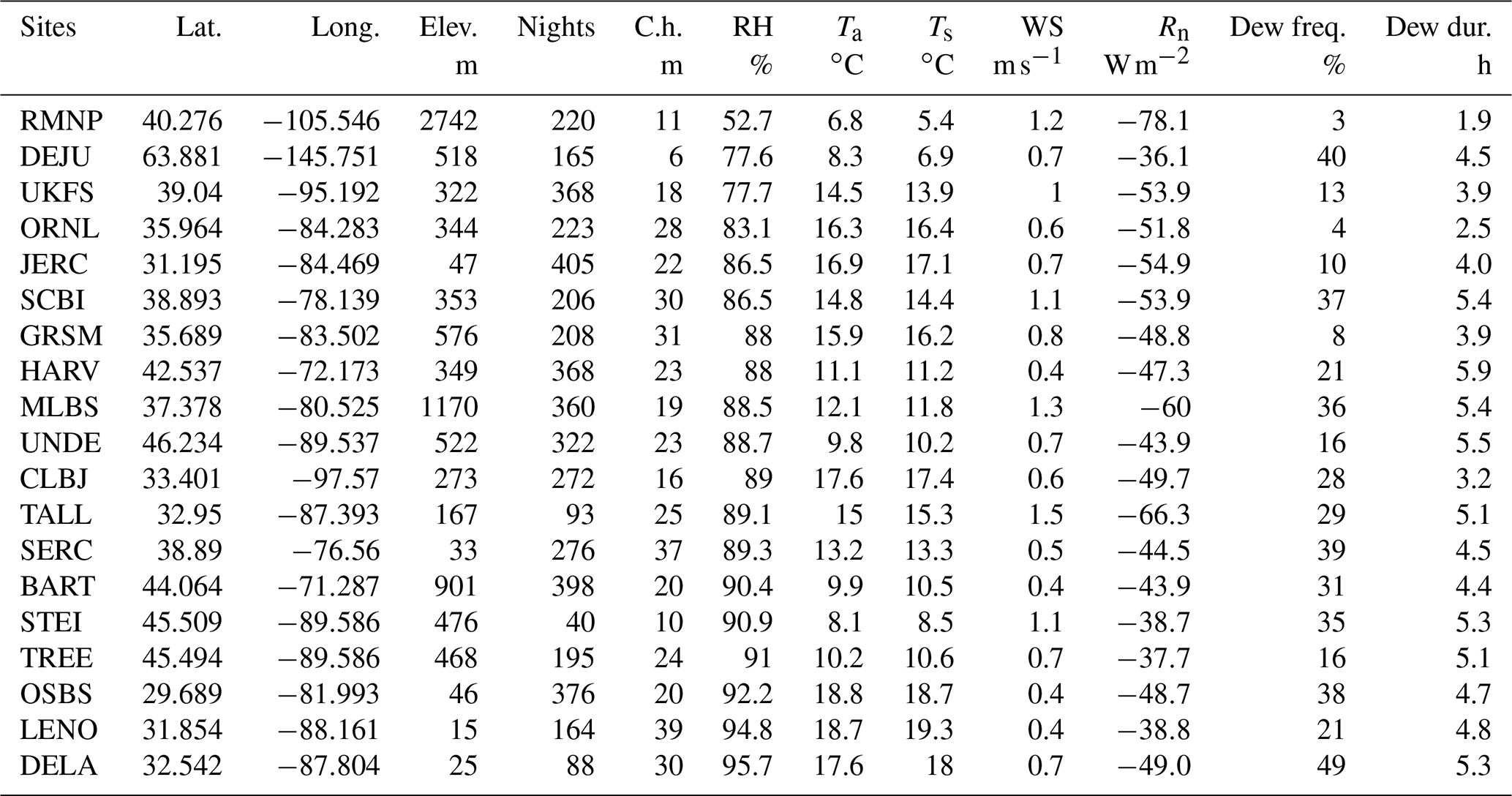
Table 2Summary of the results for the forested sites ordered with an increasing RH. Dew frequency, duration and meteorological parameters (averaged from 23:00 to 05:00 the next day) have been calculated within canopy, except Rn (above canopy). C.h. stands for canopy height, and elev. stands for elevation.
Definition of a dew event, dew duration and dew frequency. A 30 min dew event occurs when Ts≤Td (time window from 16:00 to 10:00 the next day), the dew duration per night is the summation of 30 min dew events during the night, the dew duration per site is the mean value of the strictly positive dew durations per night and the dew frequency is the percentage of the number of dewy nights (nights with at least one dew event of 30 min) compared to the total number of nights (Tables 1 and 2). In Figs. 6–8, the meteorological parameters are averaged during the dew event (i.e., over the dew duration), while in Figs. 2–4 they are averaged from 23:00 to 05:00 the next day.
Calculation of the dew yield, latent heat flux and sensible heat flux for the grasslands. To estimate the dew yield, latent and sensible heat flux, we must calculate the aerodynamic resistance to vapor transport rav between the surface and the air, which depends on the wind speed, canopy height and atmospheric stability in the Monin–Obukhov similarity theory (MOST). Our work is based on the computation of the Bulk Richardson number, which is an indicator of the atmospheric stability and is defined as the ratio of buoyancy production divided by the shear production:
where g (m s−2) is gravity, θa is the potential temperature of the air (K) at height z (m), θs is the potential temperature of the top of the canopy (K), u is the wind speed (m s−1) at height z and z0h is the roughness length for heat (m). The value of z0h has been estimated following the classical assumptions (Garratt, 1992):
with z0v and z0m being the roughness lengths for vapor and momentum (m), hc being the canopy height, and d being the displacement height (both m). Standard values are γ1=0.3 and . Empirical flux–gradient relationships between RiB and stability parameters are then used to compute the integrated stability functions for momentum and vapor, which lead to the estimate of rav (for a detailed calculation, see Jacobs et al., 2006). The latent heat flux (LE; W m−2), sensible heat flux (H; W m−2) and dew yield (M; mm) are then computed on a 30 min timescale using the following equations:
with ρa and ρw as the density of air and water (kg m−3), L as the latent heat of condensation (m2 s−2), q as the specific humidity (with sat standing for saturated; unitless), Cp as the specific heat capacity (), rav as the aerodynamic resistance (s m−1) for heat or vapor transport (commonly assumed to be similar), and τ as the length of a time step (here 30×60 s, with the factor 1000 to convert M into mm). The sign convention for H and LE (and any flux of energy) is positive when the grasslands receive energy. So, during a dew event, H>0 and LE >0 per definition. It is important to note that the work of Jacobs et al. (2006) does only concern grasslands because the aerodynamic resistance is not well defined within the canopy of the forests.
Nocturnal cycles (Figs. 9 and 10). The analysis on a nocturnal scale is performed on five different populations. Three populations of grasslands are based on their nighttime relative humidity: “dry” (RH<80 %; CPER, JORN, KONZ, MOAB, OAES and ONAQ), “temperate” (; DCFS, HEAL and WOOD) and “tropical” (RH>90 %; DSNY and LAJA). Two populations of forests are based on the timing of dew formation: “early” (∼21:00; DELA, SERC, STEI, BART, LENO, JERC, HARV and TREE) and “late” (∼00:00; DEJU, OSBS, MLBS, CLBJ, TALL and UNDE). Each of these five populations has been cut into two sub-ensembles: nights with the presence of at least 30 min of dew formation (left column in Figs. 9 and 10) and nights with a complete absence of dew formation (right column). For each night and for each parameter (wind, Ts, Ta, Td), the mean value from 16:00 to 10:00 the next day has been subtracted to produce nocturnal anomalies. These nocturnal anomalies have been stacked and the standard deviation has been calculated for each half-hour. Finally, we add the mean value of the previously subtracted mean values to the stack to produce the final nocturnal cycles.
Sensitivity analysis of the spatial variability of Ts on dew formation (Fig. 11). To simplify the analysis, the spatial distribution of the surface temperatures around the mean value measured by the radiometer on a 30 min timescale is assumed to be normal. We have tested the sensitivity of dew frequency and dew duration to a change in the standard deviation (σ) of the normal distribution, from 0 to 0.5. For each half-hour and for a given σ, we use a Monte Carlo simulation (or MCS; n=1000 runs) following a normal distribution around the 30 min average of Ts, and we calculate the percentage of randomized points (X %) that fall below Td among these 1000 runs. In this context, X is defined here as the percentage of the canopy receiving dew formation (see Fig. 11a). If X<5 %, we consider that no dew event is occurring for this half-hour. We finally calculate, for a given σ, the dew frequency, duration and the averaged percentage of canopy receiving dew formation (mean value of all percentages above 5 %) for the grasslands and the forests. If σ=0, the percentage of the canopy receiving dew formation is either 0 % (absence of dew) or 100 % (presence of dew) and the results are equivalent to the analysis without the MCS. When σ>0, more dew will be formed during the night, but this is on a lower percentage of the canopy.
Density plot construction (Figs. 7 and 8). Because of the high number of points in Figs. 7 and 8, a density plot is required to better visualize the signal in a two-dimensional graph. Each data point is associated with four different colors (from light grey to black) depending on the number of neighbors surrounding it. The size of the rectangle containing the neighbors is approximatively 2 % of the graph. The legend of Figs. 7 and 8d indicates the minimum and maximum number of neighbors for a given color, and these values have been chosen so that each color corresponds to 25 % of the total number of points.
3.1 Analysis for each site
3.1.1 Relative humidity, radiative cooling and temperature
The 11 grasslands and 19 forests can be characterized at night by their mean surface temperature and mean relative humidity (from 23:00 to 05:00 the the next day) over the growing season. A general positive trend is observed in Fig. 2a and is mostly explained by the effect of relative humidity on radiative cooling (Fig. 3a). Indeed, a higher water vapor content will make the air more efficient at absorbing and re-emitting longwave radiation, therefore the nighttime boundary layer will be more opaque to radiative loss, and this mechanism will keep the surface temperature warm at night. Additionally, sites with a high elevation like MOAB (1779 m), ONAQ (1662 m) and RMNP (2742 m) are associated with cold and dry air due to the low pressure. The relative humidity within the canopy of the forests is usually higher than the grasslands at night (86±9 % vs. 76±15 %, 1 SD) not only because of a denser canopy structure but also because forests occur in wetter regions than grasslands (Woodward et al., 2004). The two exceptions here are the grasslands LAJA and DSNY, which present tropical characteristics (, 1 SD).
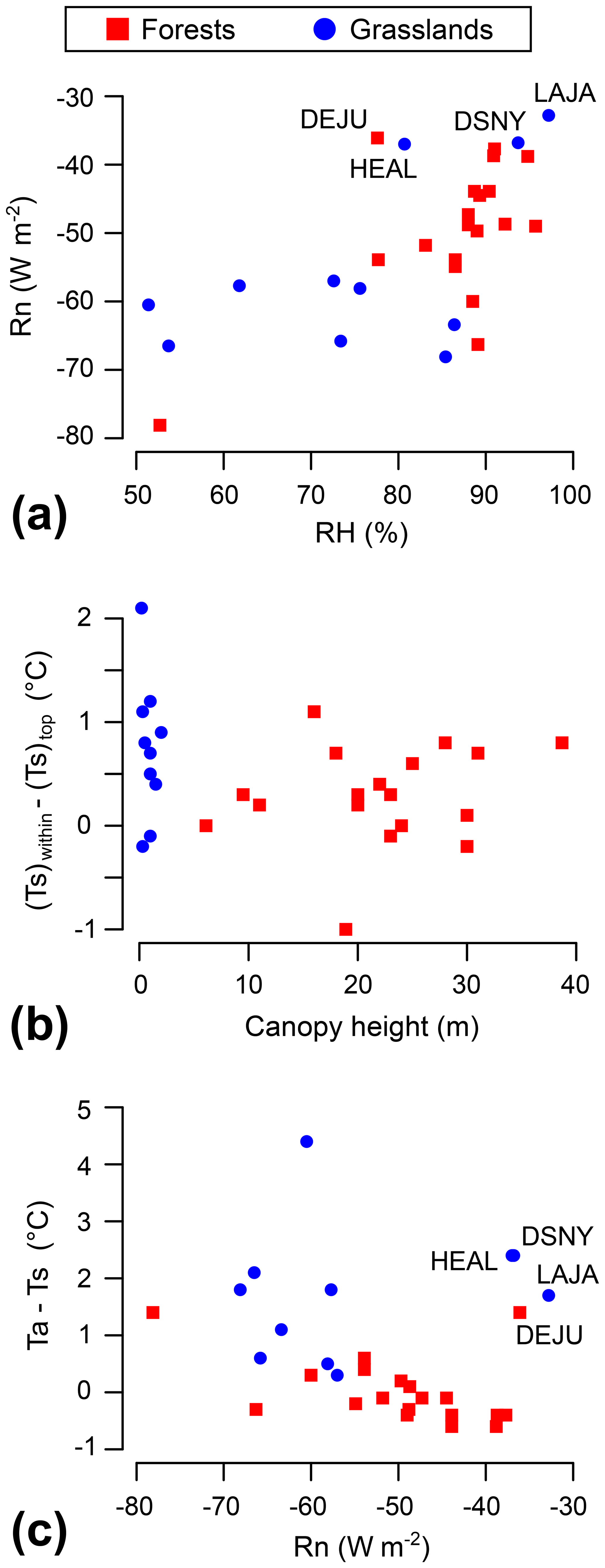
Figure 3Mean values from 23:00 to 05:00 the next day for each site over the growing season for the following parameters: Rn versus RH (a), difference in Ts between the canopy within and the top of the canopy versus the canopy height (b), and Ta−Ts (within canopy for the forests, top of the canopy for the grasslands) versus Rn (c). Four sites are selected for discussion.
Measurements performed at different heights provide the opportunity to study the vertical variability in the surface temperature and relative humidity. The difference in surface temperature between the bottom and the top of the canopy (Fig. 2b) is similar at night for the forests (, 1 SD) and the grasslands (, SD) based on a t-test (). One could consider that the vertical variability in the surface temperature at night is larger for tall-canopy ecosystems than low-canopy ecosystems because radiative fluxes are exchanged in a bigger volume. Although forests have a much higher canopy height than the grasslands (5–40 m of difference; Fig. 1), the vertical variability in their surface temperature is not larger at night. One possible explanation is that forests are wetter and have more biomass than grasslands. Their canopy will therefore cool down slower, as will the ground, because of a higher heat capacity and inefficient radiative cooling (Fig. 3a). The positive relationship observed among the forested sites in Fig. 3b seems not to be primarily driven by the canopy height. The ground flux or cloud cover data (absent from this analysis) might play an important role in the vertical gradient of surface temperature at night, as well as the vegetation density and the site wetness. Looking now at the relative humidity, it reveals to be always higher within the canopy than above the canopy for both ecosystem types (Fig. 2c). Indeed, air parcels within the canopy are not effectively mixed with drier air higher in the atmosphere (low wind speed within canopy), and the combination of soil evaporation and transpiration provides continual moisture to the canopy air space.
The difference in temperature between the air and surface (Ta−Ts) is mainly driven by radiative cooling for most sites (Fig. 3c). Interestingly, three grasslands (LAJA, DSNY and HEAL) and one forest (DEJU) with the shortest canopy height (6 m) show a large Ta−Ts despite minimal radiative cooling (Fig. 3c). These four sites do not belong to the same population: HEAL and DEJU are both located in Alaska (cold and dry air), while LAJA and DSNY are tropical (warm and wet air). Moreover, HEAL and DEJU are the only two sites that are not part of the trend in the relationship between Rn and RH (Fig. 3a). It is not clear at this point what drives these sites away from the otherwise strong relationship. The ground flux could act as a sink of energy at night for these four sites and could decrease the temperature of the canopy, which would consequently reduce the radiative cooling. Another explanation could be that nocturnal atmospheric dynamics such as the presence of warm convection above the canopy (increasing the difference in temperature) associated with an opaque cloud cover (drastically reducing the radiative cooling, even if the relative humidity is below 85 % for HEAL and DEJU; see Fig. 3a). Our current data are not sufficient to verify these hypotheses, and further investigations are required to understand what is driving Ta−Ts when the radiative cooling is weak. In a study using RDCs in tropical areas (Tahiti and Tikehau, French Polynesia), Clus et al. (2009) observe that the relative humidity impacts the efficiency of the radiative cooling, however these sites cannot be compared to LAJA or DSNY because of the presence of strong winds, a much lower relative humidity (∼80 % at night compared to ∼95 %) and the absence of surface temperature data except for one night.
3.1.2 Dew frequency, duration and yield across sites
The most frequent location where dew forms is on the top of the canopy of grasslands, which is much cooler than the ground (Fig. 2b), and within the canopy of the forests, where the relative humidity is much higher than above the canopy (Fig. 2c). Indeed, the dew frequency within the canopy of the grasslands is only 7 % compared to 29 % at the top of the canopy (DSNY and LAJA are excluded because of their tropical characteristics). For forested sites, dew forms only 11 % of the nights at the top of the canopy of the forests compared to 25 % within canopy, although the position of the RH sensors above the canopy for the forests is far away from the top of the canopy (difference of ∼15 m), which is why dew frequency at the top of the canopy might be underestimated for the forested sites. This study will therefore focus on the dew formation at the top of the canopy of the grasslands and within the canopy of the forests only.
The grassland sites show a large gap in temperature between the air and the surface at night (Fig. 3c). Consequently, the main limitation of dew formation at the top of the canopy of the grasslands will be the relative humidity. A threshold of RH=75 % separates two patterns for the dew frequency in the grasslands (Fig. 4a): (i) a low and constant dew frequency of ∼15 % of nights for RH<75 % and (ii) a linear increase in dew frequency with rising relative humidity (slope of 3.5, r2=0.92, p value <0.01) for RH>75 %. We have isolated three populations of grasslands based on their relative humidity: dry (six sites with RH<80 %), temperate (three sites with ) and tropical (two sites with RH>90 %). The dry, temperate and tropical sites have a dew frequency of 15±6 % (1 SD), 59±4 % (1 SD) and 95±4 % (1 SD), respectively. This dew frequency versus relative humidity relationship revealed by several grasslands with different climatic conditions has not yet been reported in the literature for the following reasons: the former dew studies were limited to one or two sites; there is a lack of standardized measurements between them; there is an absence of continuous humidity measurements or a decision to not report them (Xiao et al., 2009); and finally the sites are mostly chosen for their high nocturnal RH, especially in arid areas close to a coast (Zangvil, 1996; Muselli et al., 2009; Moro et al., 2009; Uclés et al., 2014; Maestre-Valero et al., 2015). The in situ radiometric network from NEON has not been specifically designed to work in locations with high dew yield, and thus the data provide information on sites that span a continuum from exceptionally low dew frequencies to an almost nightly occurrence. However, former dew studies focusing on a single site have reported a similar RH threshold value below which dew has a low probability of forming: RH=78 % in Wang et al. (2017c) (204 nights in a semi-arid site in China using leaf wetness sensors) and RH=75 % in Guo et al. (2016) (166 nights in a cold desert in China using eddy-covariance data). Even if the linear relationship in Fig. 4a is strong, the relative humidity alone is not sufficient for predicting dew frequency with a good accuracy (the residuals have a standard deviation of 10 %), which highlights the role of canopy structure and wind speed in dew formation (Sect. 3.2). See Beysens (2018) for a detailed explanation of the relationship between dew formation and relative humidity.
As mentioned in the previous sections, forested sites have a higher relative humidity within canopy than the dry and temperate grasslands at night (Fig. 2a) but a lower air–surface temperature gap (Fig. 3c). The relationship between dew frequency and relative humidity within the canopy can still be considered to be linear for RH>80 % (Fig. 4a; slope of 2.3), but with a much lower coefficient of determination (r2=0.31) because the inefficient radiative cooling or very low wind speed within canopy are also limiting dew formation in these ecosystems. Forests have a mean dew frequency of 25±14 % (1 SD), which is between the dry and temperate grasslands. Interestingly, the forest DEJU is consistent with the linear relationship calculated from the population of grasslands (Fig. 4a), which is certainly because it has the shortest canopy height (6 m) among the forested sites. Dew formation is less well documented in forested sites than arid areas or croplands and/or grasslands, possibly because small inputs from dew are not likely to have a significant impact on these ecosystems or because their tall canopies are considered as a natural radiative barrier to dew formation. However, Hao et al. (2012) reported a dew frequency of 73 % over 142 nights using eddy-covariance data in a hyper arid forest (canopy height 8–10 m, forest coverage of 50 %, and annual rainfall of 35 mm). The much higher dew frequency might be explained by the short canopy height, the low vegetation density, the presence of a river close to the area of study or simply the poor performances of the eddy-covariance method at night (de Roode et al., 2010). Unfortunately, nighttime relative humidity measurements are not available and cannot be compared with our study. In a sparse elm wood site (unknown canopy height, forest coverage of 40 % and annual rainfall of 385 mm), Wang et al. (2017a) measured a dew frequency of 54 % over 80 nights using weighing methods, a value which is much more consistent with our data. Again, relative humidity measurements are not available for the period of study.
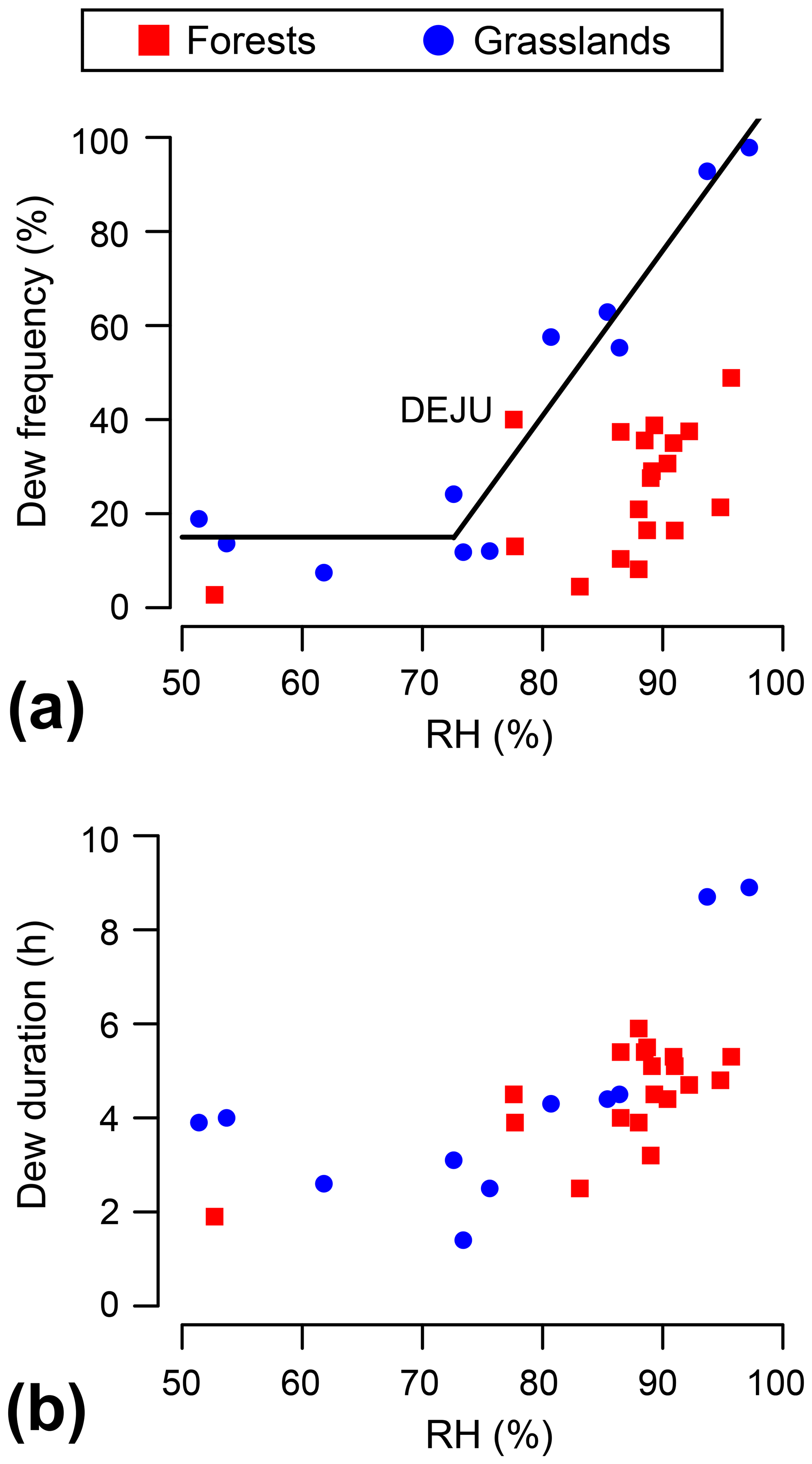
Figure 4Dew frequency (a) and duration (b) versus RH (from 23:00 to 05:00 the next day) for each site over the growing season. The slope of 3.5 (r2=0.92) in (a) has been calculated based on the grasslands with RH>70 % only. Dew formation has been calculated at the top of the canopy of the grasslands and within canopy of the forests only.
We define dew duration as the time during which the dew point temperature is above the surface temperature at night. The dry and temperate grasslands have a dew duration of 3.4±1.1 h (1 SD), and the forests have a duration of 4.5±1.1 h (1 SD). A comparison with former studies is difficult because of the varying range of dew duration in the literature: from 1–4 h (Pan et al., 2010; Hao et al., 2012) to 4–6 h (Wang et al., 2017a) or above 6 h (Moro et al., 2009; Uclés et al., 2014; Guo et al., 2016) depending on the climatic conditions, canopy structure and measurement protocol. Dew duration is positively affected by the relative humidity (Fig. 4b), but it is also sensitive to a change in wind speed (see Sect. 3.2 for a detailed analysis of the sensitivity of dew duration to these parameters). The two tropical grasslands (LAJA and DSNY) show a much higher mean dew duration (8.8±0.1 h, 1 SD) compared to the rest of the sites (Fig. 4b). Both have high nocturnal relative humidity (, 1 SD) with a surprisingly high difference in temperature between the air and the surface of the canopy at night (, 1 SD), despite having the most inefficient radiative cooling due to the saturated air (see Fig. 3c). As previously mentioned, this result needs further investigation to be fully understood, but it does not look unrealistic, as former studies have reported longer dew durations, for example 9.6±3.2 h (1 SD) in a coastal steppe over a 4-year period (Uclés et al., 2014). However, measurements of relative humidity in extremely wet conditions are notoriously difficult, and these data could be associated with a sensor failure.
So far, two robust results (dew frequency and dew duration) have been presented and calculated based on the sign of Td−Ts, without needing to consider atmospheric stability, which is essential for estimating the dew yield (expressed mm night−1). The dew yield estimation for the grasslands is based on the calculation of the aerodynamic resistance to vapor transport, which depends on many variables and is therefore prone to more uncertainties. Figure 5a shows the dew yield versus dew duration relationship using the nightly average data of the grasslands, and only one site (DSNY) failed to produce a realistic dew yield (usually below 1 mm night−1). DSNY is a tropical site with frequent rain and fog events that might largely contribute to its nocturnal water balance and reduce the performance of the MOST, even if the dew duration and frequency of DSNY are consistent with the other tropical site (LAJA). A quadratic curve (, ) fits remarkably well for the dew yield versus dew duration (r2=0.94, p value <0.01) for the other grassland sites (Fig. 5b). The fit has been calculated on 22 median values (30 min resolution on a dew duration below 11 h), and the mean value of the residuals (nightly data) is (1 SD, 575 nights). A similar quadratic pattern can be observed in the relationship of dew yield versus dew duration for two croplands (Meng and Wen, 2016) using a flux-profile method and the MOST, but the authors did not perform a regression analysis for comparison. The quadratic nature of the relationship can be qualitatively explained by the fact that the vapor pressure deficit (q(Ta)−qsat(Ts) in Eq. 1) is positively related to the dew duration. This can be seen in Fig. 7b, knowing that . Per definition, the dew yield is the integral of the dew flux over the night or is more visually the area below the dew flux curve. This area is roughly equal to the dew duration multiplied by the mean dew flux, which is driven by q(Ta)−qsat(Ts) and also depends on the dew duration as explained above. For example, if the dew duration is divided by 2, the mean dew flux will approximatively be divided by 2 as well, and the area will therefore be divided by 4, which explains the quadratic nature of the relationship.

Figure 5Dew yield versus dew duration for the grasslands (top of the canopy, nightly timescale). (a) shows the failure of the Monin–Obukhov Similarity Theory for DSNY, which is why the quadratic fit () has been calculated for the other grasslands based on the 30 min median values for dew durations between 1 and 11 h (b).
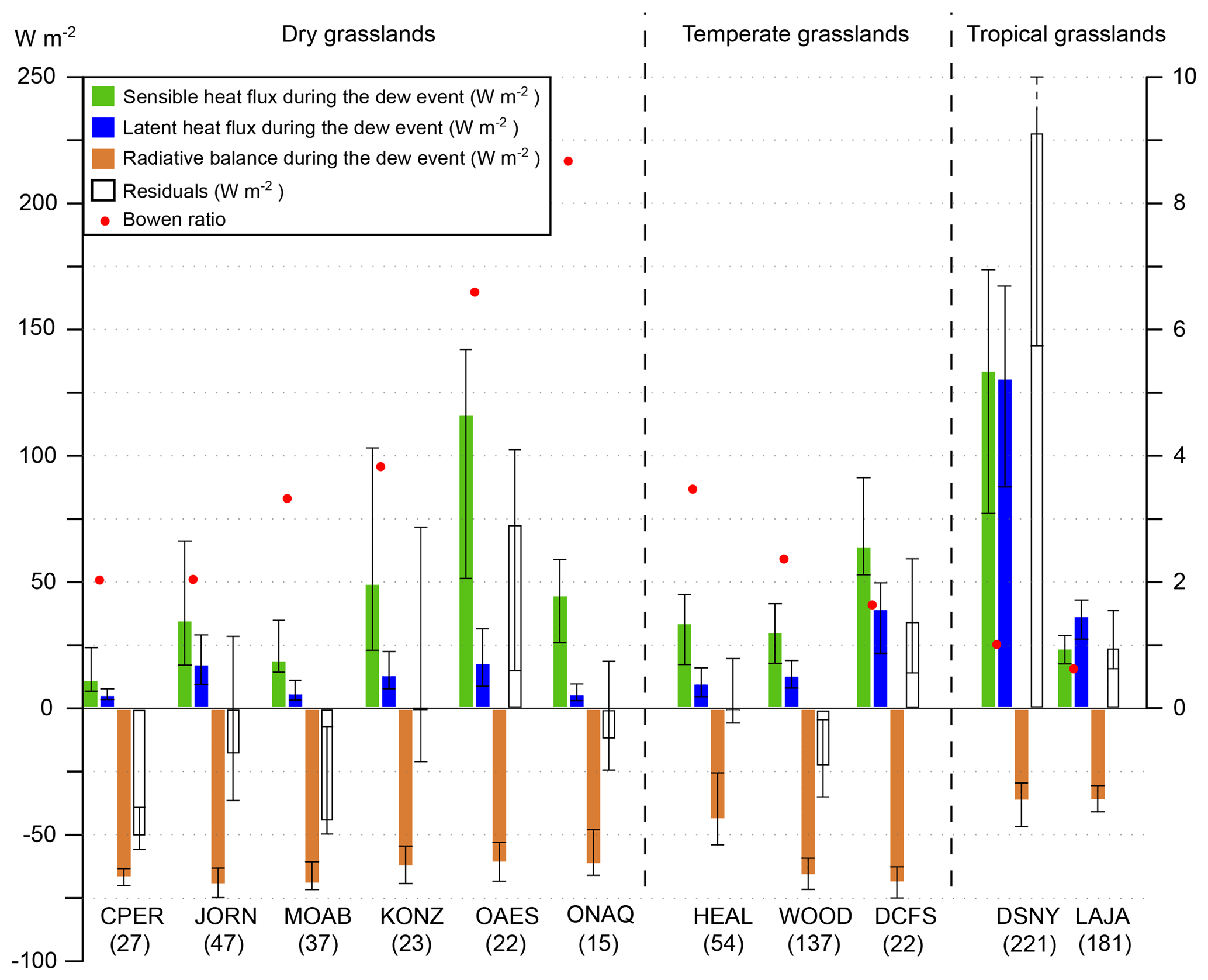
Figure 6Median value and [25,75] % quantiles (error bars) of the net radiation above canopy (Rn), and the sensible (H) and latent heat fluxes (LE) averaged during a dew event for each dewy night (indicated in parenthesis). The sign convention is positive when the grassland receives energy, and the residuals are , with Rn measured and LE and H calculated with the Monin–Obukhov similarity theory.
The mean dew yield of the dry and temperate grasslands is (1 SD), which is consistent with the 25 studies collecting dew on RDCs (, 1 SD; see Tomaszkiewicz et al., 2015), and this provides strong support for the fact that the MOST produces an accurate estimation of the dew yield based on radiometric surface temperatures. The mean dew yield of the tropical site LAJA is 0.52 mm night−1, which is high, but frequent fogs might be included in this budget because of the exceptionally low vapor pressure deficit at LAJA (saturated air and large difference in temperature between the surface and the air). In a study based on weighing methods, Pan et al. (2010) showed a significant change between dew yields forming in foggy conditions () and non-foggy conditions () that supports our result. Additionally, the maximum dew yield measured by high precision lysimeters in two temperate grasslands reached 0.5–0.6 mm night−1 (Xiao et al., 2009) for six nights. These events were associated with meteorological conditions that might occur frequently in LAJA.
3.1.3 Estimation of three energy components during dew formation in grasslands
The importance of dew formation in the nocturnal energy budget is poorly documented because of the technical challenge in measuring fluxes from eddy covariance during periods of low turbulence. Opinions differ, from dew being a negligible component of the energy budget that cannot be distinguished from the noise (de Roode et al., 2010) to dew being a process that significantly participates in the energy budget and helps to better constrain the energy closure (Jacobs et al., 2008). In this section, we compare the value of the sensible heat flux (H; W m−2), latent heat flux (LE; W m−2) and net radiation above the canopy (Rn; W m−2) associated with a dew event. See the Method section to understand how H and LE were calculated with the MOST.
Our system is a grassland (biomass above ground, roots excluded), and the energy budget is described as a volume energy balance:
with S as the energy storage within the system (W m−2) and G as the ground flux (W m−2); here the term of advection has been neglected. The volume energy balance is calculated only during a dew event and the sign convention is for positively considering an incoming flux to the system. In this case, H and LE are always positive because a dew event is associated with the condensation of water vapor on a surface (LE >0), which can only happen when the air is warmer than the surface (H>0). Figure 6 shows the median value (error bars: 25 % and 75 % quantiles) of each energy budget component for each site (number of dewy nights indicated in parenthesis), with the residuals being equivalent to S−G.
The uncertainties associated with the MOST are high at night and sensitive to not only the gradient of temperature between the air and the leaf but also to the wind speed and stability of the atmosphere. For this reason, the discussion here will be only based on the order of magnitude of the components, and DSNY will be excluded from the analysis (see Fig. 5a). In the following, we use the 50 %[25 %,75 %] quantile notation. A typical latent heat flux released by dew formation is for the grasslands (excluding LAJA and DCFS). The sensible heat flux for the same eight sites during dew formation is 3 times larger than LE and is associated with a higher variability (), while the net radiation is twice as important as the sensible heat flux (). For the tropical site LAJA, the latent heat flux can reach and stays above the sensible heat flux (). The Bowen ratio (defined as H∕LE) might therefore decline below 1 during dew events in exceptionally wet sites (nighttime RH>90 %).
As we will see in Sect. 3.3, the leaf temperature is rarely increasing during dew formation, despite the latent heat and sensible heat fluxes bringing energy to the system. The continuous decrease in leaf temperature means that the storage term S is negative during the night. The residuals (S−G) shown in Fig. 6 are positive for three sites: OAES, DCFS and LAJA. This result suggests one of the following: (i) the ground flux G is an important sink of energy (at least ) for these sites at night and/or (ii) H and LE are overestimated and the MOST fails to partition the energy budget for these sites at night. This study will not be able to validate or invalidate these two hypotheses. However, we can confirm the preliminary work of Jacobs et al. (2008) and affirm that the latent heat flux released by dew formation is a non-negligible component in the nocturnal energy budget, with a typical Bowen ratio of ∼3 during a dew event, similar to the results reported by Meng and Wen (2016) for two croplands using a flux-profile method (69 and 128 dewy nights, Bowen ratio of 1–3 in presence of dew).
3.2 Sensitivity of dew duration to meteorological parameters on a nightly timescale
The relationship between dew duration and RH (Fig. 7a), Td−Ts (Fig. 7b) or wind speed (Fig. 8) is tested by assessing all data from the network of sites on a nightly timescale. These meteorological parameters have been averaged over the dew duration for each dewy night, and their optimum values associated with long dew durations (6–15 h) will be calculated using the 50 %[25 %,75 %] quantile notation. We do not consider dew events longer than 15 h, because we expect that direct solar radiation rapidly cancels dew formation. For example, LAJA has a maximum darkness duration of ∼14 h on the study period (based on shortwave measurements).
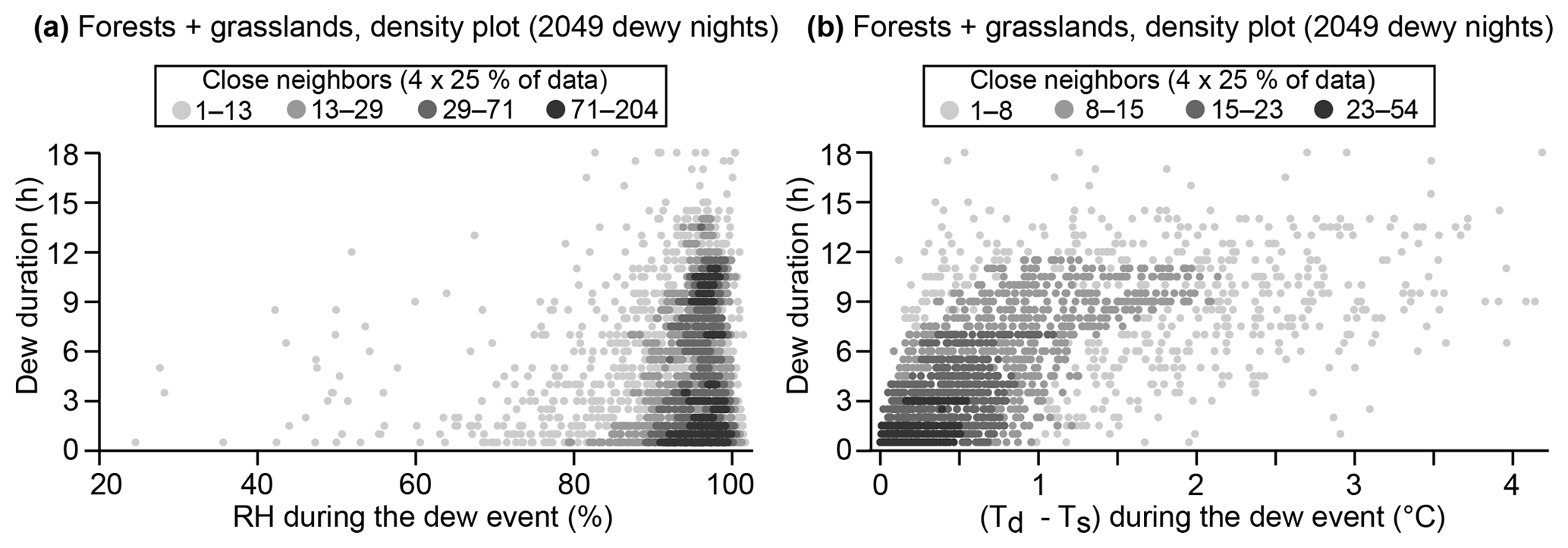
Figure 7Density plot on a nightly timescale of the dew duration versus relative humidity (a) and dew duration versus Td−Ts (b), both averaged over the dew duration (all sites included). Four shades of grey indicate the number of neighbors around a data point in a small rectangle (∼2 % of the figure). Each shade of grey represents 25 % of the total number of nights.
For both ecosystems, 98 % of the dew events occur with a relative humidity above 60 % (2049 dewy nights). The maximum dew duration during the night is limited by the relative humidity and contained in a triangular envelope (Fig. 7a), as it has been shown using RDC sensors (Muselli et al., 2009; Lekouch et al., 2012; Maestre-Valero et al., 2015; Beysens, 2016). However, in these studies, the relative humidity was averaged over the night instead of the dew duration. The higher time resolution of our data and the diversity of the grassland and forested sites offer the opportunity to calculate the optimum value of RH to form dew. For long dew durations (between 06:00 and 15:00 h), the median relative humidity is 96[93,98] %. It is remarkable to see that saturated air (RH=100 %) is not beneficial to dew formation because of the reduction of radiative loss under saturated conditions, as previously discussed. We also report the relationship between dew duration and Td−Ts (Fig. 7b), as previous studies have not had access to direct surface temperature measurements. A positive relationship can be observed when , meaning that longer dew events are associated with larger dew fluxes, which explains the quadratic pattern observed in Fig. 5b. However, the dew duration does not depend on Td−Ts anymore when because it is now only limited by the maximum darkness duration (timing of sunrise and sunset, depending on the latitude and the seasons). A typical value of Td−Ts for dew durations between 6 and 15 h is . The relationship between dew yield and Td−Ta (instead of Td−Ts) is drastically different because it shows a pattern with a triangular envelope (see Muselli et al., 2009; Lekouch et al., 2012; Maestre-Valero et al., 2015), highlighting the fact that air temperature is a poor proxy of the surface temperature.
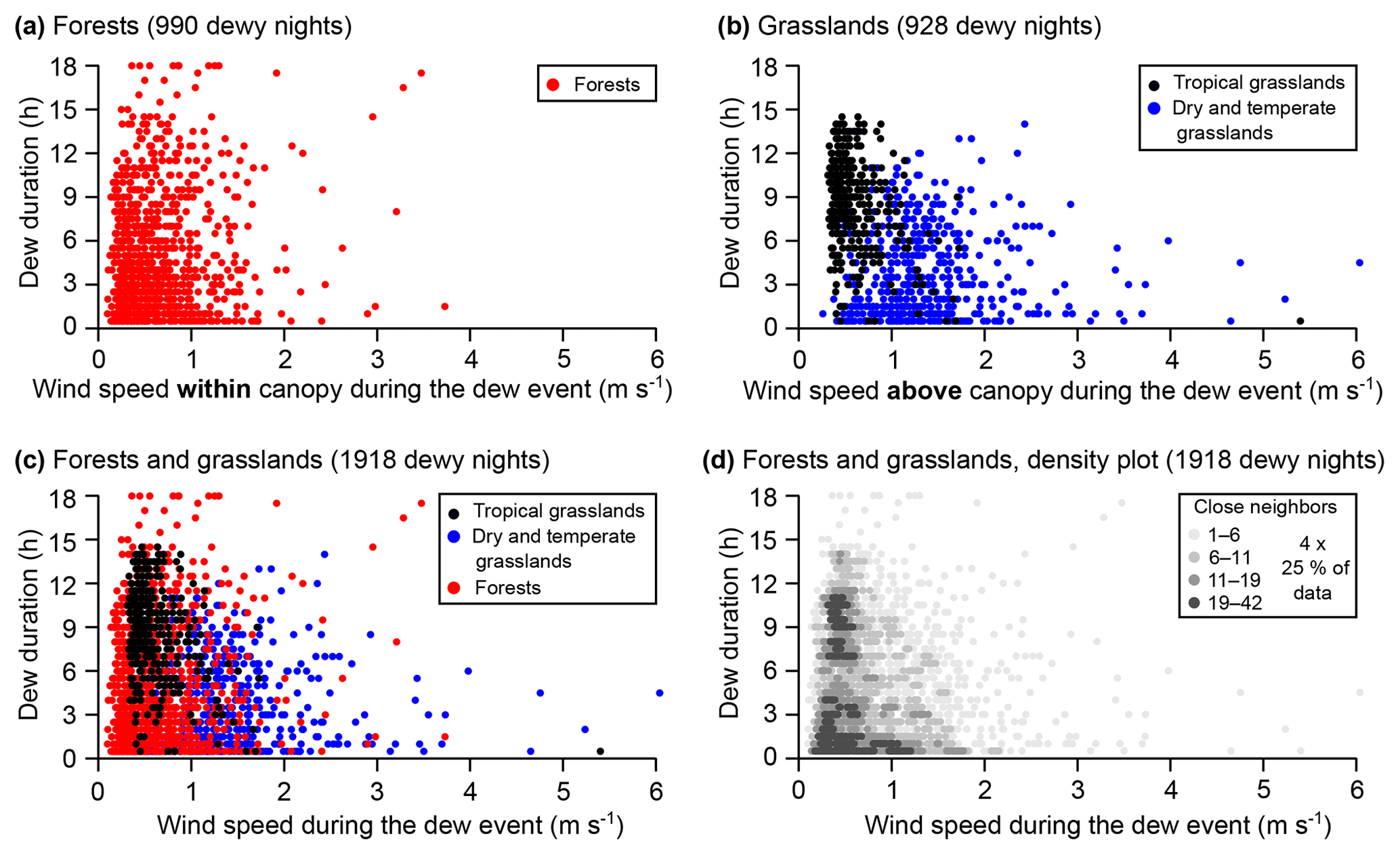
Figure 8Dew duration versus wind speed averaged during a dew event for different groups (nightly timescale): forests (a; wind speed within canopy), grasslands (b; wind speed 1 m above canopy), both of these (c) and density plot of both (d). In the density plot, four colors indicate the number of neighbors around a data point in a small rectangle (∼2 % of the figure). Each color represents 25 % of the total number of nights.
Dew is also sensitive to the wind speed, and 99 % of the dew events occur while the wind speed is below 4 m s−1 (1918 dewy nights). It is important to specify the canopy and measurement heights because the vertical logarithmic profile of the wind speed is affected by the roughness length. For the grasslands, the mean canopy height is 0.9±0.5 m (1 SD), and the mean difference between the wind speed sensor height and the top of the canopy is 0.9±0.6 m (1 SD). For the forests, as we are only interested in the dew events occurring within canopy, we averaged the wind speed measurements from all sensors below the top of the canopy (see Fig. 1) and considered this spatial average to be representative of the wind speed within canopy. The next step is to compare the relationship between dew duration and wind speed for the two following groups: within the canopy of the forests (Fig. 8a; 990 dewy nights) and at the top of the canopy of the grasslands (Fig. 8b; 928 dewy nights). Figure 8c shows graphically that the two groups exhibit a consistent triangular pattern despite various wind speed ranges, which indicates that they likely belong to the same population (Fig. 8d). As previously explained, a minimum wind speed is required to sustain dew formation by replenishing water vapor molecules in the leaf boundary layer (first part of the triangle). In contrast, strong wind speeds will equilibrate the temperature between the air and the surface at night and rapidly cancel dew formation (second part of the triangle). An optimum wind speed value is for dew durations between 6 and 15 h. The triangular envelope has been previously reported by Muselli et al. (2009), Lekouch et al. (2012) and Maestre-Valero et al. (2015) using the dew yield instead of the dew duration. Peaks in the dew yield occur at similar wind speed when the wind sensor is at 2 m ( in Maestre-Valero et al., 2015). However, when the wind speed is measured at 10 m (Muselli et al., 2009) or extrapolated to 10 m (Lekouch et al., 2012), the peak is closer to , which is comparable with our data assuming a logarithmic profile of wind speed.
3.3 Nocturnal cycles and timing of dew formation
We are now interested in the nocturnal cycles associated with the presence or absence of dew formation for three populations of grasslands (Fig. 9; dry, temperate and tropical) and two populations of forests (Fig. 10; early and late dew formation) from 16:00 to 10:00 the next day. Three simple observations that confirm what has been noted in previous sections: (i) dew rarely forms within the canopy of a grassland (Fig. 9a.1 and b.1), and it rarely forms at the top of a canopy of a forest (Fig. 10a.1 and b.1); (ii) the surface temperature, on average, does not increase during dew formation; and (iii) the top and bottom of a canopy of a forest have similar surface temperatures at night (the dashed and solid black lines are almost matching in Fig. 10). The first observation means that only the top of the canopy of a grassland cools at a sufficient rate for dew to form and that the top of a canopy of a forest is too dry for dew to form. The second observation indicates that the radiative cooling (and possibly the ground flux acting sometimes as a sink of energy) is more important than the combined warming effects of condensation (associated with LE) and friction (associated with H) on a leaf during a dew event. The third observation means that forests have a higher heat capacity as well as a higher water vapor content that redistributes radiative energy more efficiently and therefore makes the surface temperatures more homogeneous at night. Another explanation could be that a downward convection occurs from the crown level in stable conditions, therefore reducing the surface temperature difference via a sensible heat exchange (Bosveld et al., 1999).
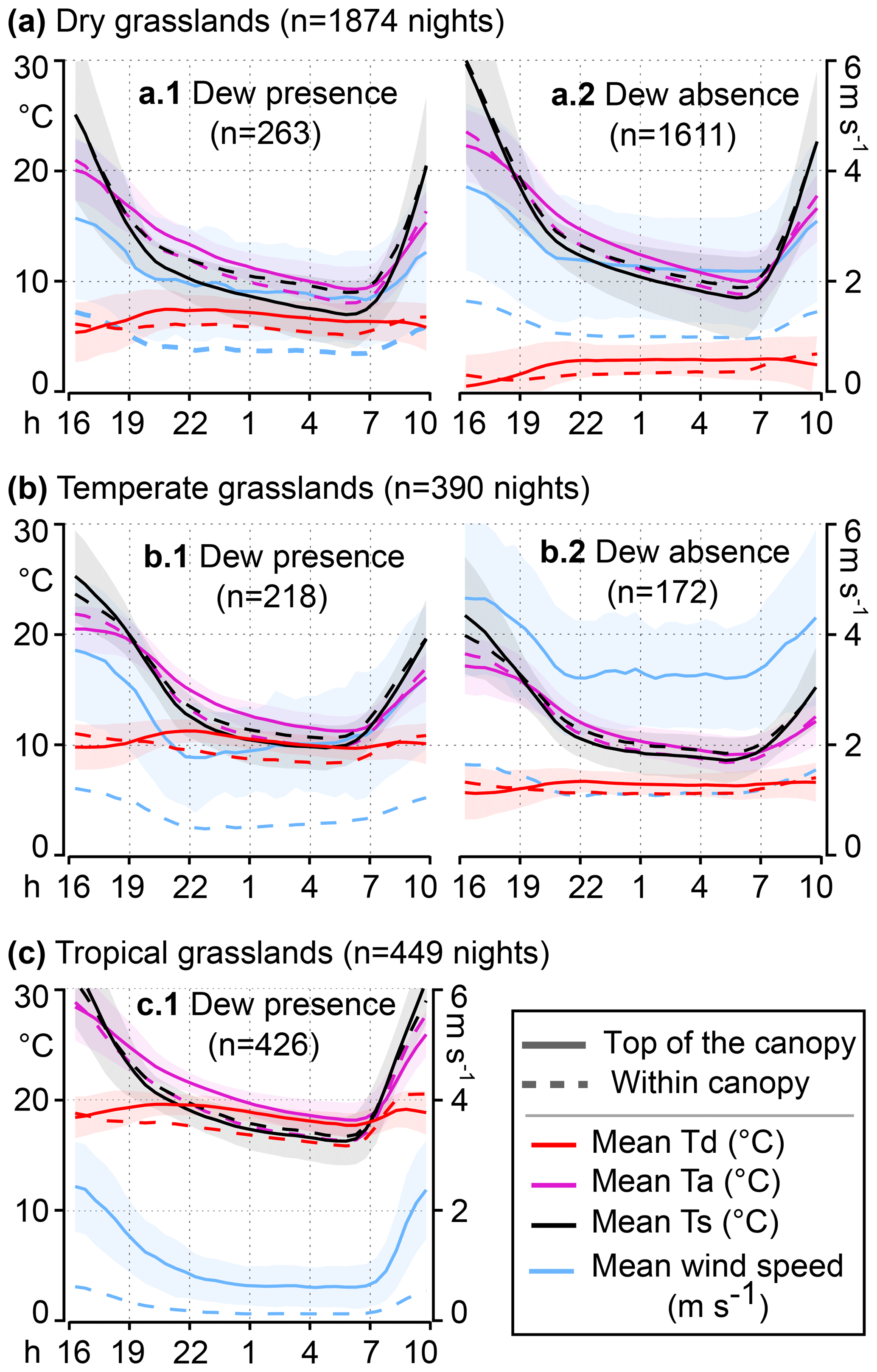
Figure 9Nocturnal cycles for three populations of grasslands with the mean value of meteorological parameters calculated on a stack of n nights (n indicated in parenthesis). The solid lines represent the top of the canopy, and the dashed lines represent within canopy. The shaded areas indicate ±1 standard deviation of the mean, shown for the top of the canopy only (for visualization purposes). (a.1), (b.1), and (c.1) are based on nights with dew formation, and (a.2) and (b.2) are based on nights without dew formation. (c.2) is missing because of a sample size that is too small.
In the following, we get insight into the relevant limiting factors for dew formation by analyzing the time that dew formation occurs. In the dry grassland sites (Fig. 9a.1), the relative humidity is so low that the only time window for the dew point temperature to reach the surface temperature occurs at the end of the night, when Ts approaches its minimum (around 03:00–05:00). In temperate grassland sites (Fig. 9b.1), the air is already warmer than the surface after 19:00, but it is not until midnight that the relative humidity rises above 85 % to start producing dew, which proceeds until 05:00. In tropical grassland sites (Fig. 9c.1), dew (and presumably fog) starts around 22:00 and finishes at 07:00 (∼2 h after sunrise). The population of forests with early dew formation (Fig. 10a.1) is interesting, because the relative humidity can already reach 90 % at 21:00 and allows dew to start forming. The downside of this high level of humidity is a reduced rate of radiative cooling from 23:00 to 05:00 by 20 % compared to the other population shown in Fig. 10b.1 ( compared to ). This stops dew formation at because the surface temperature gets too warm compared to the air temperature. Finally, the population of forests (Fig. 10b.1) will only produce dew formation from 00:00 to 05:00.
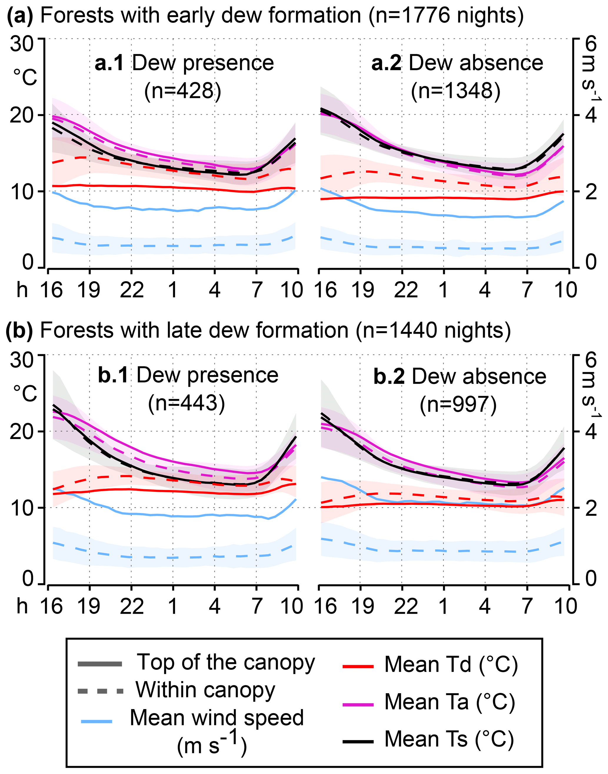
Figure 10Nocturnal cycles for two populations of forests with the mean value of meteorological parameters calculated on a stack of n nights (n indicated in parenthesis). The solid lines represent the top of the canopy, and the dashed lines represent within canopy. The shaded areas indicate ±1 standard deviation of the mean, shown within the canopy only (for visualization purposes). (a.1) and (b.1) are based on nights with dew formation, and (a.2) and (b.2) are based on nights without dew formation.
The limitation of dew formation for the grasslands (Fig. 9a.2 and b.2) is plain: the lower relative humidity yields a low dew point temperature, and the higher wind speed enhances the sensible heat exchange so that the air and the surface approach equivalent temperatures. An analysis with similar results based on nocturnal cycles can be found in two studies (Meng and Wen, 2016; Zhuang and Zhao, 2017). However, the limitation of dew formation for the forests (Fig. 10) is less clear. The wind pattern within canopy is always the same () and the relative humidity from 23:00 to 05:00 is still high for Fig. 10a.2 and b.2 (88 % and 86 %). The major reason for the absence of dew formation in Fig. 10a.2 and b.2 is the low temperature difference between the air and the surface (within canopy), and this cannot be explained by the wind pattern nor the radiative cooling. Indeed, from 23:00 to 05:00, the net radiation above the canopy is similar for Fig. 10a.1 vs. a.2 ( vs. , 1 SD) and is slightly different for Fig. 10b.1 vs. b.2 ( vs. , 1 SD). Two important unknowns here are the cloud coverage, which will reduce the efficiency of the radiative cooling, and the ground flux, which will usually bring heat to the canopy. Further investigations on the relationship between surface temperature and air temperature in forested sites at night will be required to solve this problem.
3.4 Sensitivity of dew formation to the spatial variability of the surface temperature
Because the IR radiometer provides an average temperature for the surface of the canopy, we recognize that it may underestimate dew production because of the presence of cold points on the surface. Limited work that has been done using thermal imagery of canopies (Kim et al., 2018) has shown that during the day, temperature can vary by multiple degrees based on the surface properties (e.g., the trunk, branches or dry soil versus wet soils or leaf surfaces). We do not have constraints on the temperature distribution associated with each IR temperature measurement because these spatial patterns depend on the architecture of the canopy, the wind speed, the stability of the atmosphere, the humidity and the plant type. Our assumption in this paper will be that the temperature range is distributed normally around the measured average, and we will test the sensitivity of dew frequency by varying the magnitude of the standard deviation of the normal distribution (from σ=0, with no spatial variability, to σ=0.5, with high spatial variability). For example, a IR radiometer measures at 02:00 from the top of the canopy of a grassland, while the dew point temperature of the air is . Per definition, there is no dew formation (Td<Ts) if we assume that there is no spatial variability in the surface temperature (σ=0), however 16 % of the canopy will receive dew formation for σ=0.2 based on a Monte Carlo Simulation (Fig. 11a).
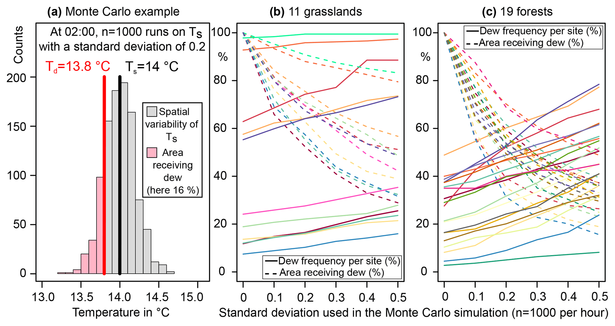
Figure 11Sensitivity of dew frequency to the spatial variability in the surface temperature based on a Monte Carlo simulation run on each half-hour data point (n=1000 runs). The spatial variability is assumed to follow a normal distribution, and only a certain percentage of the canopy will receive dew formation (example for a, 16 % at 02:00). The Monte Carlo simulation has been run with different standard deviations (from 0 to 0.5) for each half-hour for all grasslands (b) and all forests (c). A non-dew event is defined here as less than 5 % of the canopy receiving dew formation; then all the areas above 5 % have been averaged for each site (dashed lines). Colors allow association between the solid lines and the dashed lines for each site.
There is a linear response in the dew frequency for both the grasslands and forests to an increase in the standard deviation of the normal distribution representing the spatial variability of the surface temperature (Fig. 11b and c). The mean percentage of the canopy receiving dew formation starts at 100 % for σ=0 (all the canopy receives dew formation during a dew event when there is no spatial variability) and then decreases exponentially to 20 %–60 % for σ=0.5 depending on the wetness of the site. We consider that σ=0.2 for the grasslands (95 % of the surface temperature anomalies within ; see Fig. 11a) and that σ=0.1 for the forests (95 % of the surface temperature anomalies within ), because it has been observed that the forests have more homogeneous surface temperatures at night than dry and temperate grasslands (Sect. 3.3). For these standard deviations, a typical percentage of the canopy receiving dew formation during a dew event is 64±7 % (1 SD) for the grasslands (tropical sites excluded) and 70±9 % (1 SD) for the forests. The dew frequency increases from 29±23 % (1 SD) to 35±26 % (1 SD) for the grasslands (tropical sites excluded) and from 25±14 % (1 SD) to 29±15 % (1 SD) for the forests. The mean dew duration is minimally affected by considering the spatial variability of canopy temperatures, with a net gain of only 1 h with the highest variability (σ=0.5) for the grasslands and 1 h and 40 min for the forests. Estimates of dew formation are ultimately relatively insensitive to small variance in canopy temperature, which suggests that average values from the canopy are valuable. Variance in nighttime temperature are probably much smaller than the variance in daytime temperatures because of the lack of solar radiation and differences in surface albedo, but further analysis using thermal imaging would help in providing more realistic constraints in the distribution of temperature of the canopy at night.
3.5 Ecological implications of the results
Numerous studies have emphasized the ecological significance of dew formation, for example in the germination of seedlings (Zhuang and Zhao, 2016) or the recovery after a period of water stress (Munne-Bosch et al., 1999). The two main ecological functions of dew formations are reducing the transpiration during the early morning (Gerlein-Safdi et al., 2018b) and providing a significant source of water to water-stressed ecosystems via the foliar water uptake (Munne-Bosch et al., 1999). In the first case, the film of water deposited on the leaves will first be evaporated at dawn before the water contained in the plant fibers. It raises the relative humidity in the boundary layer of the leaf and decreases the surface temperature due to the absorption of latent heat. This temporally reduces transpiration from the plant later in the morning and afternoon. Because the ecological role of dew formation is more important in arid and semi-arid regions, our discussion will only be based on the dry grasslands. For these ecosystems, dew is more likely to form on the top of the canopy and just before dawn, when the surface temperature is at its minimum (Fig. 3a). This will prevent the deposited droplets from nighttime evaporation and will protect the highest part of canopy that is the most exposed to the sunlight. According our statistical analysis, dew events will only occur once (maximum twice) a week in these sites in the absence of a moisture source, because of a very low nighttime RH (Fig. 11b). These rare events will surely extend the survival rate of most species during a drought, but they cannot replace rainfalls. Dew is not likely to influence soil moisture for dense grasslands because of warmer soil surface temperatures. In contrast, dew mostly forms within canopy of forested sites, while the top of their canopies stays dry at night. Organisms such as epiphytes will therefore not benefit from dew formation if they are located on a top of a tree. We also hypothesize that the dew-induced transpiration–suppression effect will be emphasized in forested sites because the canopy is partially blocking the direct sunlight and the wind, therefore extending the presence of dew droplets on the leaves and soil.
Dew duration has been shown in this paper to be very sensitive to the wind speed and relative humidity on site. This raises the question of the impact of climate change and land surface use on the global dew yield. The intensification of the water cycle and the shift in the frequency of rainfalls are expected to drive changes in the surface relative humidity (Dai, 2006) and there has been a significant decrease observed in the surface wind speed in the Northern Hemisphere in the past decades (Vautard et al., 2010). The global cloud coverage will also play a role in the efficiency of the nighttime radiative cooling, and its evolution remains difficult to constrain. In parallel, for a given relative humidity, grasslands are more likely to receive dew formation than forested sites because of a more efficient radiative cooling that depends on the canopy architecture and the specific heat. A critical nighttime RH threshold is 75% for the grasslands (Fig. 4a). For example, an increase of 10% in the nighttime RH (from ∼75 % to ∼82 %) will double the dew frequency in grasslands (from ∼20 % to ∼40 % of the nights). A future analysis taking these elements into account will be required to estimate the change of dew formation over the globe and to anticipate its impact on water-stressed ecosystems that are endangered, like the Californian redwood forest, or regions that are regreening, like the Sahel (Dardel et al., 2014).
This study is the first attempt at performing an analysis of dew formation in various ecosystems using infrared radiometry from the National Ecological Observatory Network. The use of infrared radiometers in the study of dew formation was tested by Jacobs et al. (2006) for a single site, and our work emphasizes the importance of these continuous measurements for studying dew on a continental scale over a long period of time. This method is more appropriate for ecosystem studies (as opposed to dew harvesting applications) because it does not rely on artificial surfaces and therefore provides measurements that capture the seasonal and annual dynamics of natural ecosystems. Moreover, the use of radiometers allows us to bypass the technical difficulty of the surface temperature retrieval from an energy balance, which leads to a precise analysis of the sensitivity of dew formation to relative humidity and wind speed. It is always desirable to obtain direct measurements, however the difficulty of obtaining large-scale dew collection data makes this method very attractive. Because direct flux observations are absent from this study, further work will be necessary to cross-check the present analysis with actual dew measurements.
The results obtained in our analysis are consistent with the previous dew studies, in terms of dew frequency, duration and yield. Additionally, the diversity of the environmental and climatic conditions of the sites has led to the discovery of new features that have not yet been reported in the literature. The main reason is that former studies tended to focus on areas where dew yield was expected to be high and because the lack of standardized measurements made it difficult to do quantitative cross-site syntheses. Five important results emerge from our analysis: (i) dew mostly forms at the top of grasslands and within forested canopies; (ii) the dew frequency of grasslands follows a linear relationship with respect to the mean nocturnal relative humidity when it is above 75 %; (iii) the maximum dew duration does not seem to depend on the ecosystem type but requires ideal relative humidity and wind speed values (∼95 % and , respectively); (iv) dew duration and dew yield are related through a quadratic relationship; and (v) the spatial variability of the surface temperature plays an important role in the dew frequency but has only a minimal affect on dew duration. In parallel, one interesting result associated with the nocturnal energy balance remains unresolved and will need further investigation: what is driving the exceptional difference between air and surface temperatures at night for certain sites even when the radiative cooling is inefficient? The answer will help to develop our understanding of energy and water exchange at night in natural ecosystems.
Some limitations are also present in this study. Firstly, the Monin–Obukhov similarity theory is not applicable to forested sites because the dewfall occurs within the canopy and where estimating the aerodynamic resistance was not feasible. In additional, the Monin–Obukhov similarity theory produced unrealistically high estimates of yield for one tropical grassland site (DSNY). In these cases, it would be useful to use lysimeter data in order to validate the quadratic relationship between dew duration and dew yield using direct dew measurements. The other limitation of our work is the absence of data such as cloud cover, precipitation and ground flux. The cloud cover would have been useful in better understanding the radiative balance pattern. The precipitation data are interesting because rainfall is an important source of moisture and affects the surface temperature, and the ground flux is essential in closing the energy budget. These data will be updated by the National Ecological Observatory Network in the future. Finally, some gaps of several days or weeks in the study period of most sites and the absence of frost events in our analysis did not allow us to perform a seasonal analysis. This result will be interesting in a future study, as dew formation has been shown to have a seasonal cycle (Zangvil, 1996; Xiao et al., 2009), driven by the meteorological variables but also by the maximum darkness duration. After the upcoming update in the data assimilation, the network of continuous radiometric measurements built by the National Ecological Observatory Network will be essential for producing high-quality data for future global ecological studies on non-rainfall water input.
All data utilized in this study are freely available from the National Ecological Observatories Data repository (http://data.neonscience.org, last access: 10 April 2018, Battelle, Boulder, CO, USA). Processed data products generated from these data and codes in R are available upon request to the author.
FR designed the study and led the data analysis, writing and figure generation. MB assisted with study design, paper preparation and figure generation. DB assisted with data analysis and paper preparation.
The authors declare that they have no conflict of interest.
We would like to thank Josh Roberti and Morgan Jones for providing the
meta-data of the sites. The work was partially supported through NSF grant
1502776 to Max Berkelhammer.
Edited by: Anke Hildebrandt
Reviewed by: two anonymous referees
Ben-Asher, J., Alpert, P., and Ben-Zvi, A.: Dew is a major factor affecting vegetation water use efficiency rather than a source of water in the eastern Mediterranean area, Water Resour. Res., 46, 1–8, https://doi.org/10.1029/2008WR007484, 2010. a
Berkelhammer, M., Hu, J., Bailey, A., Noone, D. C., Still, C. J., Barnard, H., Gochis, D., Hsiao, G. S., Rahn, T., and Turnipseed, A.: The nocturnal water cycle in an open-canopy forest, J. Geophys. Res.-Atmos., 118, 10225–10242, https://doi.org/10.1002/jgrd.50701, 2013. a
Beysens, D.: Estimating dew yield worldwide from a few meteo data, Atmos. Res., 167, 146–155, https://doi.org/10.1016/j.atmosres.2015.07.018, 2016. a, b, c
Beysens, D.: Dew Water, River Publishers Series in Chemical, Environmental, and Energy Engineering, 2018. a
Bosveld, F. C., Holtslag, A., and Van Den Hurk, B.: Nighttime convection in the interior of a dense Douglas fir forest, Bound.-Lay. Meteorol., 93, 171–195, 1999. a, b
Boucher, J. F., Munson, A. D., and Bernier, P. Y.: Foliar absorption of dew influences shoot water potential and root growth in Pinus strobus seedlings, Tree Physiol., 15, 819–823, https://doi.org/10.1093/treephys/15.12.819, 1995. a
Burgess, S. S. O. and Dawson, T. E.: The contribution of fog to the water relations of Sequoia sempervirens (D. Don): Foliar uptake and prevention of dehydration, Plant Cell Environ., 27, 1023–1034, https://doi.org/10.1111/j.1365-3040.2004.01207.x, 2004. a
Clus, O., Ouazzani, J., Muselli, M., Nikolayev, V. S., Sharan, G., and Beysens, D.: Comparison of various radiation-cooled dew condensers using computational fluid dynamics, Desalination, 249, 707–712, https://doi.org/10.1016/j.desal.2009.01.033, 2009. a
Dai, A.: Recent climatology, variability, and trends in global surface humidity, J. Climate, 19, 3589–3606, https://doi.org/10.1175/JCLI3816.1, 2006. a
Dai, A.: Increasing drought under global warming in observations and models, Nature Climate Change, 3, 52–58, https://doi.org/10.1038/nclimate1633, 2013. a
Dardel, C., Kergoat, L., Hiernaux, P., Mougin, E., Grippa, M., and Tucker, C. J.: Re-greening Sahel: 30 years of remote sensing data and field observations (Mali, Niger), Remote Sens. Environ., 140, 350–364, https://doi.org/10.1016/j.rse.2013.09.011, 2014. a
Dawson, T. E.: Fog in the Califonia redwood forest: ecosystem inputs and use by plants, Oecologia, 117, 476–485, 1998. a
de Roode, S. R., Bosveld, F. C., and Kroon, P. S.: Dew formation, eddy-correlation latent heat fluxes, and the surface energy imbalance at Cabauw during stable conditions, Bound.-Lay. Meteorol., 135, 369–383, https://doi.org/10.1007/s10546-010-9476-1, 2010. a, b, c
Garratt, J. R.: The atmospheric boundary layer, Cambridge atmospheric and space science series, Cambridge University Press, Cambridge, ISBN 9780521467452, 1992. a
Gerlein-Safdi, C., Gauthier, P. P., and Caylor, K. K.: Dew-induced transpiration suppression impacts the water and isotope balances of Colocasia leaves, Oecologia, 187, 1041–1051, https://doi.org/10.1007/s00442-018-4199-y, 2018a. a
Gerlein-Safdi, C., Koohafkan, M. C., Chung, M., Rockwell, F. E., Thompson, S., and Caylor, K. K.: Dew deposition suppresses transpiration and carbon uptake in leaves, Agr. Forest Meteorol., 259, 305–316, 2018b. a, b
Guo, X., Zha, T., Jia, X., Wu, B., Feng, W., Xie, J., Gong, J., Zhang, Y., and Peltola, H.: Dynamics of dew in a cold desert-shrub ecosystem and its abiotic controls, Atmosphere, 7, 1–15, https://doi.org/10.3390/atmos7030032, 2016. a, b
Hao, X. M., Li, C., Guo, B., Ma, J. X., Ayup, M., and Chen, Z. S.: Dew formation and its long-term trend in a desert riparian forest ecosystem on the eastern edge of the taklimakan desert in China, J. Hydrol., 472–473, 90–98, https://doi.org/10.1016/j.jhydrol.2012.09.015, 2012. a, b
Jacobs, A. F. G., Heusinkveld, B. G., Kruit, R. J. W., and Berkowicz, S. M.: Contribution of dew to the water budget of a grassland area in the Netherlands, Water Resour. Res., 42, 1–8, https://doi.org/10.1029/2005WR004055, 2006. a, b, c, d, e
Jacobs, A. F. G., Heusinkveld, B. G., and Holtslag, A. A. M.: Towards closing the surface energy budget of a mid-latitude grassland, Bound.-Lay. Meteorol., 126, 125–136, https://doi.org/10.1007/s10546-007-9209-2, 2008. a, b
Kalma, J. D., McVicar, T. R., and McCabe, M. F.: Estimating land surface evaporation: A review of methods using remotely sensed surface temperature data, Surv. Geophys., 29, 421–469, https://doi.org/10.1007/s10712-008-9037-z, 2008. a
Kim, Y., Still, C. J., Roberts, D. A., and Goulden, M. L.: Thermal infrared imaging of conifer leaf temperatures: Comparison to thermocouple measurements and assessment of environmental influences, Agr. Forest Meteorol., 248, 361–371, 2018. a
Kosmas, C., Danalatos, N. G., Poesen, J., and Van Wesemael, B.: The effect of water vapour adsorption on soil moisture content under Mediterranean climatic conditions, Agr. Water Manage., 36, 157–168, https://doi.org/10.1016/S0378-3774(97)00050-4, 1998. a
Lekouch, I., Lekouch, K., Muselli, M., Mongruel, A., Kabbachi, B., and Beysens, D.: Rooftop dew, fog and rain collection in southwest Morocco and predictive dew modeling using neural networks, J. Hydrol., 448–449, 60–72, https://doi.org/10.1016/j.jhydrol.2012.04.004, 2012. a, b, c, d
Limm, E. B., Simonin, K. A., Bothman, A. G., and Dawson, T. E.: Foliar water uptake: A common water acquisition strategy for plants of the redwood forest, Oecologia, 161, 449–459, https://doi.org/10.1007/s00442-009-1400-3, 2009. a
Maestre-Valero, J., Ragab, R., Martínez-Alvarez, V., and Baille, A.: Estimation of dew yield from radiative condensers by means of an energy balance model, J. Hydrol., 460, 103–109, 2012. a
Maestre-Valero, J. F., Martínez-Alvarez, V., Baille, A., Martín-Górriz, B., and Gallego-Elvira, B.: Comparative analysis of two polyethylene foil materials for dew harvesting in a semi-arid climate, J. Hydrol., 410, 84–91, https://doi.org/10.1016/j.jhydrol.2011.09.012, 2011. a
Maestre-Valero, J. F., Martín-Górriz, B., and Martínez-Alvarez, V.: Dew condensation on different natural and artificial passive surfaces in a semiarid climate, J. Arid Environ., 116, 63–70, https://doi.org/10.1016/j.jaridenv.2015.02.002, 2015. a, b, c, d, e, f, g, h
Meissner, R., Seeger, J., Rupp, H., Seyfarth, M., and Borg, H.: Measurement of dew, fog, and rime with a high-precision gravitation lysimeter, J. Plant Nutr. Soil Sci., 170, 335–344, https://doi.org/10.1002/jpln.200625002, 2007. a
Meng, Y. and Wen, X.: Characteristics of dew events in an arid artificial oasis cropland and a sub-humid cropland in China, J. Arid Land, 8, 399–408, https://doi.org/10.1007/s40333-016-0006-y, 2016. a, b, c
Minnis, P., Mayor, S., Smith, W. L., and Young, D. F.: Asymmetry in the diurnal variation of surface albedo, IEEE T. Geosci. Remote, 35, 879–890, https://doi.org/10.1109/36.602530, 1997. a
Monteith, J. L.: Dew, Q. J. Roy. Meteor. Soc. 83, 322–341, https://doi.org/10.1002/qj.49708335706, 1957. a
Monteith, J. L., Szeicz, G., and Waggoner, P. E.: The Measurement and Control of Stomatal Resistance in the Field, J. Appl. Ecol., 2, 345–355, 1965. a
Moro, M. J., Were, A., Morillas, L., Villagarcia, L., Cantón, Y., Lazaro, R., Serrano-Ortiz, P., Kowalski, A. S., and Domingo, F.: Dew contribution to the water balance in a semiarid coastal steppe ecosystem (Cabo de Gata, SE Spain), in: Advances in studies on desertification, Murcia, 16–18 September, 2009. a, b, c
Munne-Bosch, S., Nogues, S., and Alegre, L.: Diurnal variations of photosynthesis and dew absorption by leaves in two evergreen shrubs growing in Mediterranean field conditions, New Phytol., 144, 109–119, https://doi.org/10.1046/j.1469-8137.1999.00490.x, 1999. a, b, c
Muselli, M., Beysens, D., Mileta, M., and Milimouk, I.: Dew and rain water collection in the Dalmatian Coast, Croatia, Atmos. Res., 92, 455–463, https://doi.org/10.1016/j.atmosres.2009.01.004, 2009. a, b, c, d, e
Pan, Y. X., Wang, X. P., and Zhang, Y. F.: Dew formation characteristics in a revegetation-stabilized desert ecosystem in Shapotou area, Northern China, J. Hydrol., 387, 265–272, https://doi.org/10.1016/j.jhydrol.2010.04.016, 2010. a, b, c
Payero, J. O. and Irmak, S.: Variable upper and lower crop water stress index baselines for corn and soybean, Irrigation Sci., 25, 21–32, https://doi.org/10.1007/s00271-006-0031-2, 2006. a, b
Richards, K.: Adaptation of a leaf wetness model to estimate dewfall amount on a roof surface, Agr. Forest Meteorol., 149, 1377–1383, 2009. a
Sánchez, J. M., Kustas, W. P., Caselles, V., and Anderson, M. C.: Modelling surface energy fluxes over maize using a two-source patch model and radiometric soil and canopy temperature observations, Remote Sens. Environ., 112, 1130–1143, https://doi.org/10.1016/j.rse.2007.07.018, 2008. a
Sánchez, J. M., López-Urrea, R., Rubio, E., and Caselles, V.: Determining water use of sorghum from two-source energy balance and radiometric temperatures, Hydrol. Earth Syst. Sci., 15, 3061–3070, https://doi.org/10.5194/hess-15-3061-2011, 2011. a
Sánchez, J. M., López-Urrea, R., Rubio, E., González-Piqueras, J., and Caselles, V.: Assessing crop coefficients of sunflower and canola using two-source energy balance and thermal radiometry, Agr. Water Manage., 137, 23–29, https://doi.org/10.1016/j.agwat.2014.02.002, 2014. a
Sentelhas, P. C., Monteiro, J. E. B. A., and Gillespie, T. J.: Electronic leaf wetness duration sensor: Why it should be painted, Int. J. Biometeorol., 48, 202–205, https://doi.org/10.1007/s00484-004-0200-z, 2004. a
Stewart, J. B., Kustas, W. P., Humes, K. S., Nichols, W. D., Moran, M. S., and Debruin, H. A. R.: Sensible Heat-Flux Radiometric Surface-Temperature Relationship for 8 Semiarid Areas, J. Appl. Meteorol., 33, 1110–1117, https://doi.org/10.1175/1520-0450(1994)033<1110:Shfrst>2.0.Co;2, 1994. a
Suleiman, A. and Crago, R.: Hourly and daytime evapotranspiration from grassland using radiometric surface temperatures, Agron. J., 96, 384–390, https://doi.org/10.2134/agronj2004.0384, 2004. a
Tolk, J. A., Howell, T. A., Steiner, J. L., Krieg, D. R., and Schneider, A. D.: Role of transpiration suppression by evaporation of intercepted water in improving irrigation efficiency, Irrig. Sci., 16, 89–95, https://doi.org/10.1007/BF00189165, 1995. a
Tomaszkiewicz, M., Abou Najm, M., Beysens, D., Alameddine, I., and El-Fadel, M.: Dew as a sustainable non-conventional water resource: a critical review, Environ. Rev., 23, 425–442, https://doi.org/10.1139/er-2015-0035, 2015. a, b
Tomaszkiewicz, M., Abou Najm, M., Beysens, D., Alameddine, I., Bou Zeid, E., and El-Fadel, M.: Projected climate change impacts upon dew yield in the Mediterranean basin, Sci. Total Environ., 566–567, 1339–1348, https://doi.org/10.1016/j.scitotenv.2016.05.195, 2016. a, b
Troufleau, D., Lhomme, J. P., Monteny, B., and Vidal, A.: Sensible heat flux and radiometric surface temperature over space Sahelian vegetation. I. An experimental analysis of the kB-1parameter, J. Hydrol., 188–189, 815–838, https://doi.org/10.1016/S0022-1694(96)03172-1, 1997. a
Uclés, O., Villagarcia, L., Moro, M. J., Canton, Y., and Domingo, F.: Role of dewfall in the water balance of a semiarid coastal steppe ecosystem, Hydrol. Process., 28, 2271–2280, 2014. a, b, c, d
Vautard, R., Cattiaux, J., Yiou, P., Thépaut, J. N., and Ciais, P.: Northern Hemisphere atmospheric stilling partly attributed to an increase in surface roughness, Nat. Geosci., 3, 756–761, https://doi.org/10.1038/ngeo979, 2010. a
Vuollekoski, H., Vogt, M., Sinclair, V. A., Duplissy, J., Järvinen, H., Kyrö, E.-M., Makkonen, R., Petäjä, T., Prisle, N. L., Räisänen, P., Sipilä, M., Ylhäisi, J., and Kulmala, M.: Estimates of global dew collection potential on artificial surfaces, Hydrol. Earth Syst. Sci., 19, 601–613, https://doi.org/10.5194/hess-19-601-2015, 2015. a, b
Wagner, W. and Pruß, A.: The IAPWS formulation 1995 for the thermodynamic properties of ordinary water substance for general and scientific use, J. Phys. Chem. Ref. Data, 31, 387–535, https://doi.org/10.1063/1.1461829, 2002. a
Wang, C., Cen, Y., Liu, M., and Bowler, P.: Formation and influencing factors of dew in sparse elm woods and grassland in a semi-arid area, Acta Ecologica Sinica, 37, 125–132, https://doi.org/10.1016/j.chnaes.2017.06.004, 2017a. a, b
Wang, L., Kaseke, K. F., and Seely, M. K.: Effects of non-rainfall water inputs on ecosystem functions, Wiley Interdisciplinary Reviews: Water, 4, e1179, https://doi.org/10.1002/wat2.1179, 2017b. a
Wang, X., Gao, Z., Wang, Y., Wang, Z., and Jin, S.: Dew measurement and estimation of rain-fed jujube (Zizyphus jujube Mill) in a semi-arid loess hilly region of China, J. Arid Land, 9, 547–557, https://doi.org/10.1007/s40333-017-0061-z, 2017c. a
Woodward, F. I., Lomas, M. R., and Kelly, C. K.: Global climate and the distribution of plant biomes, Philos. T. Roy. Soc. B, 359, 1465–1476, https://doi.org/10.1098/rstb.2004.1525, 2004. a
Xiao, H., Meissner, R., Seeger, J., Rupp, H., and Borg, H.: Effect of vegetation type and growth stage on dewfall, determined with high precision weighing lysimeters at a site in northern Germany, J. Hydrol., 377, 43–49, https://doi.org/10.1016/j.jhydrol.2009.08.006, 2009. a, b, c, d
Zangvil, A.: Six years of dew observations in the Negv Desert, Israel, J. Arid Environ., 32, 361–371, 1996. a, b
Zhuang, Y. and Zhao, W.: The ecological role of dew in assisting seed germination of the annual desert plant species in a desert environment, northwestern China, J. Arid Land, 8, 264–271, https://doi.org/10.1007/s40333-015-0014-3, 2016. a
Zhuang, Y. and Zhao, W.: Dew formation and its variation in Haloxylon ammodendron plantations at the edge of a desert oasis, northwestern China, Agr. Forest Meteorol., 247, 541–550, https://doi.org/10.1016/j.agrformet.2017.08.032, 2017. a, b