the Creative Commons Attribution 4.0 License.
the Creative Commons Attribution 4.0 License.
 | 07 Mar 2019
Conservative finite-volume forms of the Saint-Venant equations for hydrology and urban drainage
New integral, finite-volume forms of the Saint-Venant equations for one-dimensional (1-D) open-channel flow are derived. The new equations are in the flux-gradient conservation form and transfer portions of both the hydrostatic pressure force and the gravitational force from the source term to the conservative flux term. This approach prevents irregular channel topography from creating an inherently non-smooth source term for momentum. The derivation introduces an analytical approximation of the free surface across a finite-volume element (e.g., linear, parabolic) with a weighting function for quadrature with bottom topography. This new free-surface/topography approach provides a single term that approximates the integrated piezometric pressure over a control volume that can be split between the source and the conservative flux terms without introducing new variables within the discretization. The resulting conservative finite-volume equations are written entirely in terms of flow rates, cross-sectional areas, and water surface elevations – without using the bottom slope (S0). The new Saint-Venant equation form is (1) inherently conservative, as compared to non-conservative finite-difference forms, and (2) inherently well-balanced for irregular topography, as compared to conservative finite-volume forms using the Cunge–Liggett approach that rely on two integrations of topography. It is likely that this new equation form will be more tractable for large-scale simulations of river networks and urban drainage systems with highly variable topography as it ensures the inhomogeneous source term of the momentum conservation equation is Lipschitz smooth as long as the solution variables are smooth.


The one-dimensional (1-D) Saint-Venant equations (SVEs) are the simplest equations that capture the full dynamics of river and open-channel flow, and yet they are not universally used where river networks are explicitly represented in hydrological and urban drainage models. Furthermore, where the SVEs are used the numerical solution methods typically employ a non-conservative form, which inherently has greater numerical dissipation than the conservative form. But even the undesirable non-conservative form of the SVEs is rarely used for large systems – instead, reduced-physics models are common. These approaches a priori neglect some part of the flow dynamics for simpler computation (see Sects. 2 and 3 for discussions of these issues). In their call for “hyperresolution global land surface modeling”, Wood et al. (2011) postulated that the principal issues that limit SVE use in river networks could be resolved by application of more computing power and more precise river geometry. Hodges (2013) argued that there were wider challenges to using the SVEs, but these are not sufficient reasons relying on reduced-physics models that are calibrated to get the right answer for the wrong reason. In the intervening years some progress has been made toward improving applications of the SVEs, but large-scale hydrological modeling of river networks with application of supercomputer power continues to rely on reduced-physics methods (e.g., the US National Water Model, Cohen et al., 2018). Arguably, the dynamics of river flow are the most observable and should be the easiest part of hydrology to model (or at least with lower uncertainty in boundaries and forcing compared to overland or groundwater flow), so it is unsatisfactory that more than a half century after Preissmann (1961) we still are not universally using the SVEs in hydrological modeling of river networks.
The present work evolved out of a frustration with the slow pace of improvement in SVE modeling. Taking a step backwards, we can ask the following: is there something fundamental in the common forms of the SVEs that hinders progress? Motivated by an analysis of the equation forms (Sect. 2) and a study of the wealth of past work in the SVEs (Sect. 3), new insights were developed and are presented herein. The fundamental theses of the present work are as follows: (1) conservative formulation of equations should be used for the next generation of river network models, and (2) the appearance of the channel slope (S0) in the SVEs for channels with irregular topography is a principal cause of instabilities and extended computational time. Neither thesis can be demonstrated herein – this work is merely a first step that provides the theoretical foundations for a conservative and inherently well-balanced approach that highlights the minimal level of approximations needed for a SVE form with irregular topography. It remains for future studies to compare models built on these foundations to the existing approaches to determine if the new forms provide significant numerical advantages.
The new conservative form of the SVEs is developed with a goal of addressing challenges associated with modeling large-scale 1-D flow network systems. In the process of developing the new form, we will encounter a philosophical question as to whether the primary vertical variable in a large-scale network solution should be the depth (H) or the water surface elevation (η). Despite this author's prior work with H primacy (Liu and Hodges, 2014), we shall see that there are advantages to using η, which is identical to the piezometric pressure and hence uniform over a channel cross-sectional area. The quadrature of the subgrid piezometric pressure gradient and subgrid-scale topography can be handled in a single new term that is derived herein. Through this term interesting possibilities for analytically including hyperresolution bathymetric knowledge while retaining larger computational elements for large-scale modeling arise. This idea is not fully exploited within the present work, but the framework is developed for others to build upon.
In the remainder of this paper, Sect. 2 provides motivation and context in the differential forms of the SVEs. Section 3 provides a further overview of SVE modeling in the wide range of conservative and non-conservative forms. A new and complete derivation of the finite-volume form of the conservative 1-D momentum equation with minimal approximations is provided in Sect. 4. Approximate forms of the 1-D SVEs are presented in Sect. 5 and the final form of the equations and a discussion of their potential use are provided Sect. 6.
In reach-scale hydraulic studies, the Saint-Venant equations are almost always solved in a conservative form (e.g., Karelsky et al., 2000; Lai et al., 2002; Papanicolaou et al., 2004; Sanders, 2001) but usually in a non-conservative form when used in river network hydrology and urban drainage networks (e.g., Liu and Hodges, 2014; Pramanik et al., 2010; Rossman, 2017; Saleh et al., 2013). Arguably, the reasons are in the difficulty in obtaining a well-balanced model for the conservative form and the inherent complexities/uncertainties of channel geometry across a large network (see discussion in Sect. 3). In general, conservative equation forms are valued as they ensure (with careful discretization) that transport modeling does not numerically create or destroy the transported variable. Indeed, the use of the conservative form for mass conservation is universal in models from hydraulics to hydrology – it is only for momentum that the non-conservative form remains common.
To set the context for this paper, consider the non-conservative form of the momentum equation that has been used in large river network solutions (Liu and Hodges, 2014)
where Q is the flow rate, A is the channel cross-sectional area, β is the momentum coefficient (associated with nonuniform velocities integrated over A), g is gravity, H is the water depth, S0 is the channel slope, and Sf is the friction slope. The above equation has immediate physical appeal as each term represents a clearly understood piece of physics; i.e., the rate of change of the flow is affected by the gradient of nonlinear advection, the hydrostatic pressure gradient (driven by water depth), the gravitational force along the slope, and frictional resistance. The equation includes a conservative form of nonlinear advection (all the variables inside the gradient), but is non-conservative (that is, A, which is a function of H, is outside the gradient). The terms to the right-hand side (RHS) of the equal sign are considered source and sink terms that reflect creation and destruction of momentum. Thus, a conservative form of the above could be formally written as
where the trivial act of moving the pressure gradient term to the RHS is a recognition that it can cause non-conservation (source and sink) of the conserved momentum fluxes from the left-hand side (LHS). That is, any component on the RHS is capable of creating or destroying momentum, whereas the terms on the LHS (if properly discretized) cannot. The above equations can be contrasted with an equivalent momentum equation using the free-surface elevation:
which is obtained by substitution of with zb as the bottom elevation and . The equation is again conservative by virtue of including the gradient of the free-surface elevation as a source term (Ying et al., 2004; Wu and Wang, 2007; Ying and Wang, 2008). Comparison of Eqs. (2) and (3) shows how the introduction of S0 affects the equation form. Of particular note is that we expect Sf=f(Q, A), so the latter equation will have a smooth source term as long as the solution variables themselves are smooth. In contrast, the smoothness of the source term in Eq. (2) inherently depends on the smoothness of the product AS0 and compensation by the solution in and ASf. The key point is that smoothness in the source term is a mathematical necessity for the numerical solution of a partial differential equation to be well-posed (Iserles, 1996), but introduction of S0 can place smoothness at the mercy of how well the numerical scheme responds to non-smooth forcing.
In general, there is an advantage to having as much of the physics as possible included on the flux-conservative side of the equation, which helps reduce difficulties associated with discretizations of the source terms (e.g., Pu et al., 2012; Vazquez-Cendon, 1999). The standard form of the conservative SVEs is arguably the form provided by Cunge et al. (1980), based on a derivation of Liggett (1975):
where I1 and I2 are integrated hydrostatic pressure forces across the channel
and along the channel gradients
with H(x) as the water depth, B(x, z) as the channel breadth as a function of elevation and along-stream location, and z as a coordinate direction measured from a common horizontal baseline in a direction opposite to gravitational acceleration. This form is also used by others with slightly different nomenclature but the same integral terms (e.g., Hernandez-Duenas and Beljadid, 2016; Sanders, 2001; Saavedra et al., 2003). It is convenient herein to call this the Cunge–Liggett form of the SVEs. The key point for both these terms is that they measure the interaction between the free surface and the channel shape; e.g., I1 could also be written as
where zb is the channel bottom.
By comparing Eq. (4) with Eq. (2), we see that the novelty of Cunge–Liggett is in moving a portion of the from the RHS source term into the conservative flux on the LHS. Indeed, with this idea we see that Eq. (2) can be used with the product rule of differentiation to generate a slightly different conservative form:
Similar to the Cunge–Liggett form, the above uses a mathematical trick to place one part of the hydrostatic pressure force within the conservative flux gradient, while retaining the remainder as a source term. Thus, we see that the Cunge–Liggett form is not canonical, nor is it a form that necessarily better represents the physics. It is merely a form that is (sometimes) convenient for splitting the gradient of the total hydrostatic pressure force into conservative flux and non-conservative source terms.
The above brings up a question: if it is good to shift a portion of the hydrostatic pressure from the source to the conservative term as in Eqs. (4) and (8), then why not some or all of the gravitational potential associated with gAS0? Underlying the Cunge–Liggett form and much (but not all) of the literature is the idea that gAS0 is a source term that creates and destroys momentum. But this is also true of the hydrostatic pressure gradient and yet we commonly treat a portion within the convective flux. Thus, if Cunge–Liggett Eq. (4) is preferred over the baseline conservative form of Eq. (2) because a portion of the hydrostatic pressure is moved from the source term to the conservative flux term, then an equation that moves some (or all) of the gravitational potential from the source to the flux term should be equally valued. If this argument is accepted, then the preferred differential form for natural channels with the SVEs is none of those presented above, but perhaps an equation of the general form
where f1 and f2 are some functions (as yet unspecified) of the free-surface elevation rather than the depth. The free surface (η) can be interpreted as the uniform piezometric pressure over the cross-sectional area A, so the f1 and f2 functions are a generic way of splitting the piezometric pressure gradient between the source term and the conservative flux term, similar to how Cunge–Liggett handles the hydrostatic pressure gradient. Note that this proposed general approach removes the need for specifying S0, which is important both in terms of source-term smoothness and producing well-balanced methods as discussed in detail in Sect. 3, below.
In this paper, complete derivations are presented to show that finite-volume formulations of the SVEs can be generated that are consistent with the general conservative differential form of Eq. (9). The new derivation is intended to bridge the gap between approaches used in high-resolution hydraulic models and those used in large-scale hydrology and urban drainage networks. The derivation provides a form of the SVEs that has mathematical rigor while preserving the simplicity of the non-conservative finite-difference discretizations that are common in hydrological and urban drainage literature. Herein, we focus only on the detailed presentation of the new equation form, reserving demonstration in a numerical model to future papers.
3.1 Origination and use of the SVEs
The original equations of de Saint-Venant (de Saint-Venant, 1871) were written as
where U is the velocity, ℓp is the wetted perimeter, and F is the frictional force per unit bottom area along the channel, and other terms are as previously noted. We have taken the liberty of replacing Saint-Venant's notation of w, ζ, χ, s with the more modern nomenclature of A, η, ℓp, x, but otherwise have retained the original form. The momentum equation of de Saint-Venant, Eq. (11), is identical to Eq. (1) if we use Q=AU, , integrate over a cross section with the β coefficient, apply some calculus with the continuity equation, and define along with . From a practical perspective, the only thing that a hydrologist really needs to change from the original equation set is to replace the zero on the right-hand side of Eq. (10) with a source term representing the inflow/outflow per unit length from/into the catchment and groundwater. However, from a numerical modeling perspective, Eq. (11) is fundamentally non-conservative and suitable only for discretization in finite-difference forms. Although the full equation set is sometimes called the SVEs, for convenience in exposition we will use SVE as a shorthand for the momentum equation alone.
The SVEs are ubiquitous in the literature for a wide range of work and have a foundational role in flow-routing schemes in hydrological models and channel network models for urban drainage. However, there is an interesting gap between the equation forms used in large-scale systems and those used in shorter single-reach studies or modeling hydraulic features. For computational simplicity, large-scale network flow models often use a reduced set of equations, such as the Muskingum, kinematic wave, or the local inertia form (e.g., Wang et al., 2006; David et al., 2011, 2013; Getirana et al., 2017). Herein, we will follow the arguments of Hodges (2013) that we should be using the full SVEs; i.e., reduced-physics models should be seen as a stopgap measure as we wrestle with obtaining satisfactory SVE solution methods. As computational power has increased, our large-scale models have been moving towards the full SVEs but typically in a non-conservative form (e.g., Paiva et al., 2013; Liu and Hodges, 2014). For urban drainage networks, the US EPA Storm Water Management Model (SWMM) and variants built on this public domain model use a non-conservative finite-difference form of the SVEs. This model is widely applied (e.g., Gulbaz and Kazezyilmaz-Alhan, 2013; Hsu et al., 2000; Krebs et al., 2013); however deficiencies in conservation are a recognized problem (Rossman, 2017) and the SVE solver is the critical computational expense in the modeling system (Burger et al., 2014). Engineering river hydraulics problems are often solved using the US Army Corps of Engineers HEC-RAS software, which has free model executables with a proprietary (closed-source) code base. HEC-RAS uses a non-conservative finite-difference form of the SVEs based on methods pioneered in last quarter of the 20th century (Brunner, 2010). In contrast, more recent research models of the SVEs at short river-reach scales have typically used the equations presented as hyperbolic conservation laws that ensure both conservation and well-behaved solutions for subcritical, supercritical, and transcritical flows (e.g., Guinot, 2009; Ivanova et al., 2017; Papanicolaou et al., 2004; Sanders et al., 2003).
There is also a vast gulf between the spatial discretization of SVEs for large systems and smaller system studies in the hydraulics and applied mathematics literature (although the gap is getting narrower). For example in 2003 the SVEs were solved at 1 to 4 km spacing for 156 km of river (Saavedra et al., 2003). Seven years later we find 4 km cross-section spacing for 5×10³ km of river (Pramanik et al., 2010). By 2014 the state of the art was 100 m spacing for 15×103 km of river (Liu and Hodges, 2014). In contrast, hydraulic studies have typically focused on 1 to 10 m spacing for 1 to 2 km test cases (e.g., Gottardi and Venutelli, 2003; Kesserwani et al., 2009; Sart et al., 2010; Venutelli, 2006). Between these extremes, single-reach river models with natural geometry are typically modeled over river lengths less than 20 km with grid cells on the order of 10 m to more than 100 m (Sanders et al., 2003; Catella et al., 2008; Castellarin et al., 2009; Lai and Khan, 2012).
3.2 Preissmann vs. Godunov
Computational modeling of the SVEs is arguably a long-running contest between the differential, finite-difference governing equations pioneered by Preissmann (1961) and the integral, finite-volume formulations derived from Godunov (1959). Clearly this is a simplification as there are wide-ranging contributions across both numerical methods and implementation schemes – but the literature is simply too broad to discuss all developments in anything less than a book. Nevertheless, using a dialectic of Preissmann vs. Godunov is a useful way of thinking about the major developments and providing context for the equations derived herein. Preissmann developed effective finite-difference methods applied to the non-conservative form of the equations, which is the first basis for comparison of succeeding finite-difference models. The introduction of Roe's approximate Riemann solver (Roe, 1981) and analyses of Harten et al. (1983) made Godunov-like methods tractable and set off a multi-decadal development of finite-volume methods. The literature with these two methods is vast, but a reasonable cross section is provided in Table 1. Beyond these two major families, a variety of other schemes have been applied including finite-element methods (e.g., Szymkiewicz, 1991; Venutelli, 2003), finite-volume methods that do not use the Godunov approach (e.g., Audusse et al., 2004, 2016; Catella et al., 2008; Katsaounis et al., 2004; Mohamed, 2014; Vazquez-Cendon, 1999; Xing and Shu, 2011; Ying et al., 2004), and finite-difference methods that do not apply the Preissmann scheme (e.g., Abbott and Ionescu, 1967; Aricò and Tucciarelli, 2007; Buntina and Ostapenko, 2008; Schippa and Pavan, 2008; Tucciarelli, 2003; Wang et al., 2000). A recent development is the introduction of discontinuous Galerkin (DG) methods, which can be thought of as a higher-order Godunov method (e.g., Kesserwani et al., 2008, 2009; Lai and Khan, 2012; Xing, 2014; Xing and Zhang, 2013).
It is clear from the above that there is no consensus on the best method for solving the SVEs. For high-resolution modeling that correctly preserves shocks and transcritical flows, it can be reasonably argued that finite-volume and DG schemes are more successful than finite-difference schemes. Beyond that broad observation, the question of whether a finite-volume method with a Godunov-like approach is better than a non-Godunov approach does not have a clear answer either in terms of accuracy or computational run times. However, in terms of large-scale systems the Preissmann scheme and finite-difference methods presently reign supreme with the ability to solve more than 15×103 km of river on a desktop computer (Liu and Hodges, 2014). Nevertheless, we can see that a conservative finite-volume approach for large-scale systems would be preferred as the basis for simulating continental river dynamics (Hodges, 2013) as well as for the challenges of urban drainage modeling for the megacities that are growing across the earth. Being able to control numerical dissipation of momentum and ensure conservative fluxes will be increasingly important as advancing computing power pushes down the practical model grid scales.
Canelon (2009)Bollermann et al. (2013)Casas et al. (2010)Delis and Skeels (1998)Castellarin et al. (2009)Delis et al. (2000b)Chau and Lee (1991)Delis et al. (2000a)Chen et al. (2005)Ferreira et al. (2012)Gasiorowski (2013)Gottardi and Venutelli (2003)Islam et al. (2008)Goutal and Maurel (2002)Leandro and Martins (2016)Greenberg and Leroux (1996)Liu and Hodges (2014)Guinot (2009)Lyn and Altinakar (2002)Ivanova et al. (2017)Paiva et al. (2011, 2013)Kesserwani et al. (2010)Paz et al. (2010)Kurganov and Petrova (2007)Rosatti et al. (2011)Li and Chen (2006)Saavedra et al. (2003)Liang and Marche (2009)Sart et al. (2010)Monthe et al. (1999)Saleh et al. (2013)Pu et al. (2012)Sen and Garg (2002)Sanders (2001)Venutelli (2002)Sanders et al. (2003)Wu et al. (2004)Venutelli (2006)Zeng and Beck (2003)Wu and Wang (2007)Zhu et al. (2011)Ying and Wang (2008)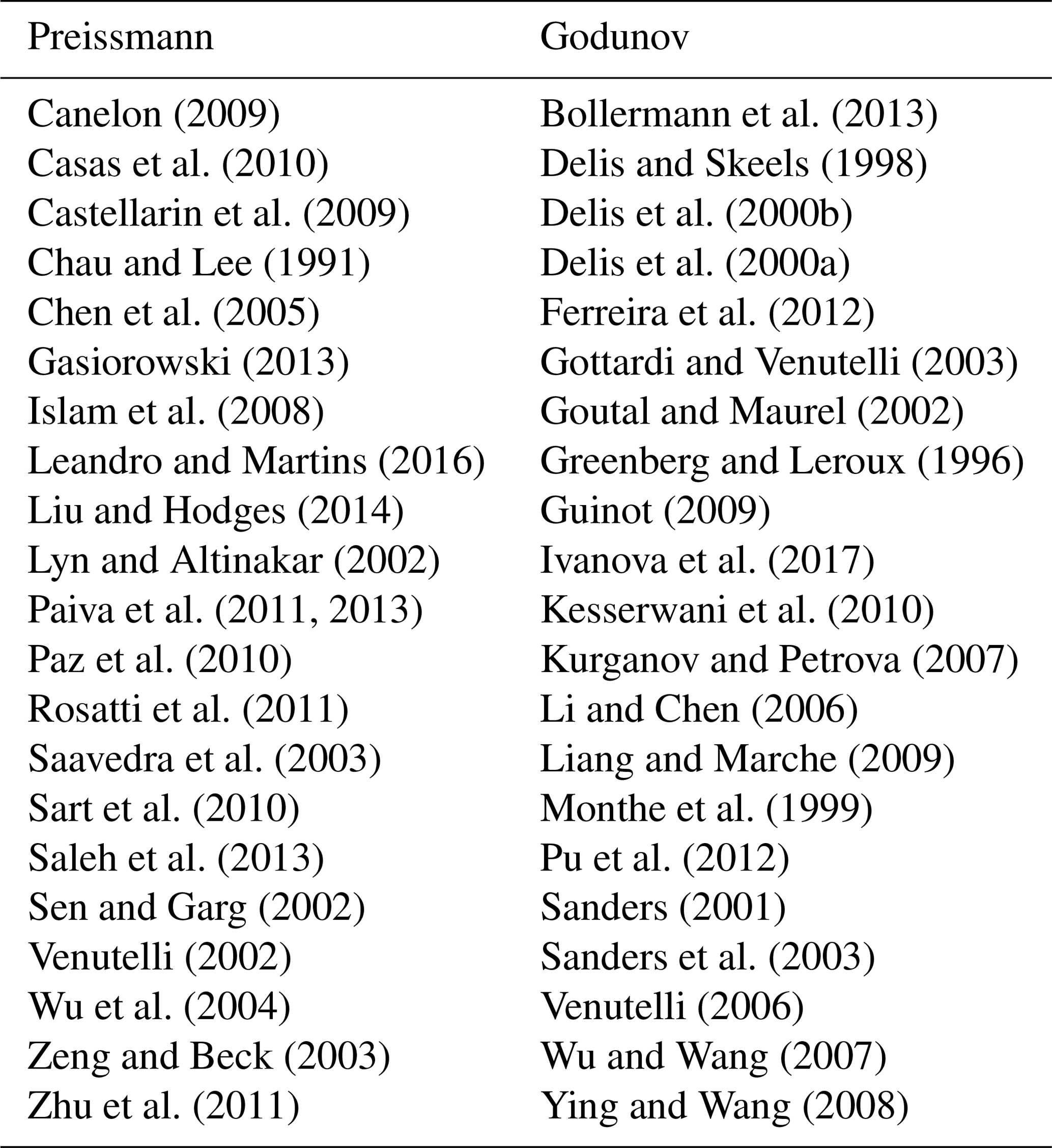
3.3 The well-balanced problem and S0
That finite-volume solutions are not commonly used in large-scale hydrologic and urban drainage models is a testament to their complexity. The difficulties associated with finite-volume solutions using the Cunge–Liggett conservative form of the SVEs have engendered a broad literature on well-balanced schemes – also known as schemes maintaining the “𝒞-property” – as derived in the study of Greenberg and Leroux (1996). A principal feature of a well-balanced scheme is that it provides exactly steady solutions for exactly steady flows. The most trivial requirement (which is often not met by unbalanced schemes) is that a flat free surface should result in exactly zero velocities. This problem is readily illustrated by considering Eq. (4) with Q=0, which implies Sf=0. Achieving the simple result of a flat free surface for Q=0 with the Cunge–Liggett form requires
which implies the Cunge–Liggett form is only well-balanced if the geometry meets the following identity at every possible water surface level:
where ηmax is the maximum water surface elevation, zb(x) is the local channel bottom elevation, and zR encompasses all possible water surface elevations. Clearly, designing a numerical scheme that exactly preserves this relationship for nonuniform channels is a challenge, as evidenced by the breadth and complexities of studies focused on this issue (e.g., Audusse et al., 2004; Bollermann et al., 2013; Bouchut and Morales de Luna, 2010; Castro Diaz et al., 2007; Crnković et al., 2009; Kesserwani et al., 2010; Kurganov and Petrova, 2007; Li et al., 2017; Liang and Marche, 2009; Perthame and Simeoni, 2001; Xing, 2014). Failure to satisfy the well-balanced criteria results in models that generate spurious velocities; i.e., a mismatch in Eq. (13) indicates that the numerics provide momentum sources and sinks that are functions of channel shape and discretization rather than flow physics. An interesting approach to this problem was developed by Schippa and Pavan (2008), where Eq. (12) is used to replace I2+AS0 in the source term with evaluated for a horizontal surface. Their approach ensures that any discretization will be well-balanced for a zero-velocity flow.
The work of Schippa and Pavan (2008) and review of other works on well-balanced schemes provide us with a key insight: the principal challenge for obtaining a well-balanced method is the channel bottom slope, S0, which is often sharply varying or even discontinuous in a natural system. Furthermore, as a geometrical property, S0 should be independent of the cross-sectional flow area (A), and yet is forced to be discretely related through Eq. (12). If we take this idea a step further, we can argue that the fundamental problem with the Cunge–Liggett form is that the physical forces that alter momentum (gravitational potential and hydrostatic pressure) are arbitrarily separated so that one is wholly within the source term and the other has an ad hoc split between conservative flux and source terms. Thus, we return to the idea put forward in the introduction that we should consider the free-surface elevation (piezometric pressure) instead of the water depth (hydrostatic pressure) as our primary forcing gradient.
In the next section, we shall see how the idea of shifting portions of the total piezometric pressure from source to flux can be used to develop a rigorous, conservative, and well-balanced finite-volume form of the SVEs that is simpler than those based on the Cunge–Liggett form.
4.1 Continuity
Although we are focused on the momentum equation, for completeness we will start with continuity. The general arrangement of the control volume for an irregular channel and the vectors used in the following discussion are illustrated in Fig. 1. Applying only the incompressibility approximation for a uniform-density fluid, the volume-integrated continuity equation is
where the Einstein summation convention is applied on repeated subscripts, uk is a vector velocity, nk is a unit normal vector defined as positive pointing outward from a control volume V, and SV is a volume source (SV<0 for a sink).
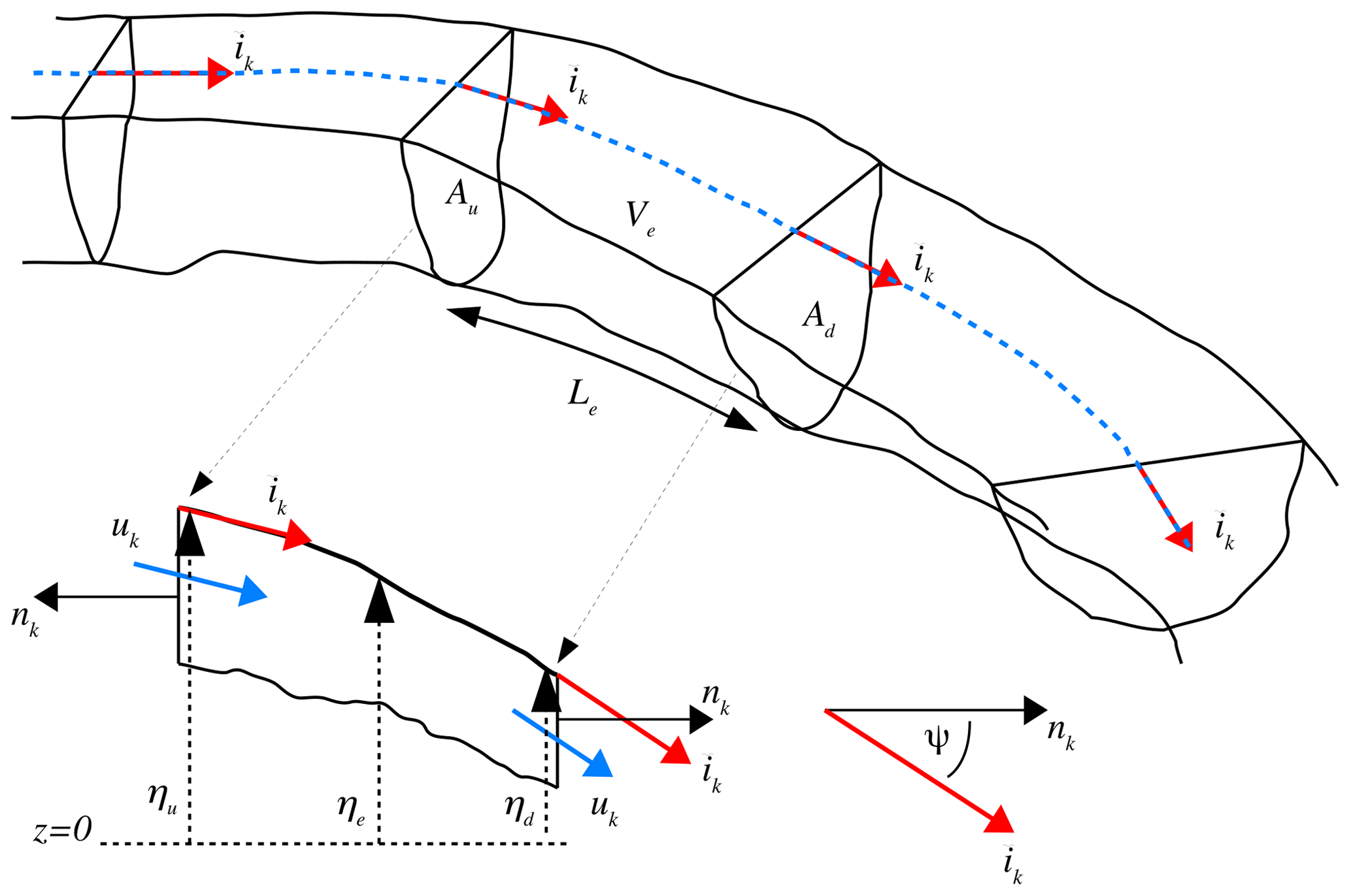
Figure 1General arrangement of control-volume element (Ve) and its neighbors for the irregular channel. Unit normal vectors nk are always perpendicular to cross-sectional areas (Au, Ad) and pointing outward from control volume. The element length (Le) is measured along the channel. Unit vectors are coincident with the free-surface slope in the streamwise direction and can be defined as local continuous functions. The velocity vector uk is approximated as parallel to . The angle measured from nk to is ψ. The free-surface elevations ηu, ηe, and ηd are cross-section uniform elevations at the upstream face, for the element center, and the downstream face, respectively. Note that volume is V throughout the derivations with u and U used for continuous and spatially averaged velocities, respectively.
A semi-discrete finite-volume representation of continuity can be directly written as
where Q and L represent the flow rate and element length, and subscripts “e”, “u”, and “d” denote characteristic values for the control-volume element, nominal upstream face, and nominal downstream face, respectively. Here we use the nominal flow direction as the global downhill direction of the channel that is assigned at the network level. The average lateral inflow per unit length is qe, and a flow Q>0 is from the upstream to downstream direction. Reversals of flow from the nominal flow direction are handled with Q<0.
4.2 Momentum
The control-volume form of the Navier–Stokes momentum equation in a direction defined by unit vector in a Cartesian frame is
where is a velocity vector component in the direction (i.e., the direction that is a priori of interest), uk represents velocity components along Cartesian axes, the component of the gravity vector in the direction is , the kinematic viscosity is ν, and p represents the thermodynamic pressure. Note that this formulation can be related to any arbitrary Cartesian axes. In many common derivations, is approximated as coincident with an x axis that is a horizontal vector in the streamwise direction. In the following, we will show that this approximation is not required. Instead, we treat this as a simplification that can be applied to the final equation form.
4.3 Advection terms
The direction for momentum, Eq. (16), is a vector associated with the velocity, which is not necessarily coincident with the normal vector nk at a flux surface of a finite volume (in contrast to the case where is taken as horizontal). For a gradually varying open-channel flow we can take the vector as the nominal downstream direction along the channel centerline described by a vector that lies along the free surface, as illustrated in Fig. 1. Thus, this vector is local (as opposed to being forced into coincidence with a Cartesian axis) and changes along the channel with the slope of the free surface. It follows that a discrete control-volume formulation developed from Eq. (16) can be globally exact as Ve→0. In contrast, a derivation that takes as a vector in the horizontal direction has a momentum conservation error proportional to cos ψ, where ψ is an angle between the horizontal vector and the free surface; such an error does not vanish as Ve→0 unless the free surface is flat across the length of the element. This idea helps illustrate one of the subtle implications of the Godunov approach in which the channel is imagined as having a piecewise flat free surface: cos ψ=1 is then an identity within the approximation of the physics rather than an approximation within the mathematics.
For Eq. (16), the upstream element face is required to be vertical and normal to the smooth channel centerline in a horizontal plane, as illustrated in Fig. 1. The free surface at the centerline has an angle of ψ(x) to the horizontal so that the discrete nonlinear momentum term in the direction across the upstream face is formally
where Q is the flow rate, is the average streamwise velocity over the cross-sectional area, the “u” subscript indicates the upstream face (rather than vector components), and β is the momentum coefficient for the streamwise velocity, defined as
Note that the only approximation in the convective term of Eq. (17) is that the streamwise velocity is parallel to the free surface. However, the interpretation of the and uknk terms may not be obvious, so further explanation is provided in Appendix A. For notational convenience, it is useful to let . However, since , strictly speaking this requires an unconventional Q=AUcos ψ. If the channel is straight and the free surface is linear so that the upstream face is parallel to the downstream face and there is a single value of ψ, it follows that an exact finite-volume integration of the nonlinear advection term is
where Me represents any integrated sources (+) and sinks (−) of momentum per unit mass in the finite-volume element associated with the qeLe lateral fluxes of Eq. (15). Note that Me terms are typically neglected in SVE solvers. For the more general case where the channel is curved between the upstream and downstream faces and the free-surface gradient changes (as in Fig. 1), the above integration becomes an approximation that is only exactly satisfied in the limit as the control-volume length goes to zero. For present purposes, the use of a gradually varying streamwise direction implies that pressure is perfectly redirecting momentum through bends and aligning the momentum with the free surface. These are (generally) unstated approximations used in common 1-D SVE formulations. However, it should be noted that this perfect momentum redirection is not precisely correct; e.g., secondary circulation in bends affects bed shear, velocity distribution, and frictional losses (Blanckaert and Graf, 2004). Arguably, losses associated with flow redirection in channel bends and/or rapid changes in the free-surface gradient should be built into the frictional term in any model. Unfortunately, this remains a relatively poorly studied area at the interface of hydrology and hydraulics. The curvature effects on the equations can be written as perturbation terms that relate the channel width to the radius of curvature (Hodges and Imberger, 2001; Hodges and Liu, 2014), but these ideas have yet to be exploited in developing curvature effects in SVE numerical models.
4.4 Pressure decomposition
For the pressure term in Eq. (16) we follow the traditional approach for incompressible flows of defining a modified pressure () that includes the gravity term, which requires . More formally we define
The surface integral for the modified pressure decomposes into integrations over the upstream cross section (Au), the downstream cross section (Ad), the channel bottom (AB), and the free surface (Aη) as
Note that AB includes both the bottom and side walls (if any). The above is an exact pressure term without imagining the geometry to be rectilinear or that the free surface has any simplified shape. The only geometric requirement of the volume is that faces Au and Ad must be vertical planes that cut across the channel, which is necessary for consistency with the convective term. The first simplification we can introduce is to approximate the free surface as uniform at any cross section. The slope of the free surface is then coincident with the vector everywhere, which is aligned with the free surface at the channel centerline. With the free surface aligned with , the modified pressure is normal to the free surface everywhere and cannot contribute to the streamwise momentum (which we have defined as parallel to in deriving the advection terms, above). It follows that is identically zero at the free surface and the last term in Eq. (21) vanishes.
4.5 Piezometric and non-hydrostatic pressure
It is convenient to introduce a decomposition of the modified pressure () into a piezometric pressure (P) and non-hydrostatic pressure (), where only the latter is nonuniform over a cross section. The non-hydrostatic pressure is defined by the difference between the modified pressure and the piezometric pressure:
The piezometric pressure is formally the sum of the hydrostatic pressure and the gravitational potential at any point z for , which provides P(x, y, z)≡ρg[η(x, , y). For the SVEs, the free-surface elevation can be considered uniform over the channel breadth (i.e., neglecting cross-channel tilt in channel bends). It follows that the piezometric pressure is
which is uniform over a vertical cross section. The non-hydrostatic pressure was neglected by de Saint-Venant and arguably should be neglected in any 1-D momentum equation bearing his name. However, for completeness we retain the non-hydrostatic pressure terms in the derivation below but neglect them in discrete forms of the piezometric pressure terms in Sect. 5.
4.6 Pressure on flow faces
To further simplify the first two pressure terms in Eq. (21), we define ψ(x) as the angle between a horizontal line and the free surface, η(x), measured clockwise positive from the horizontal line pointing downstream. Thus, the vector is generally at an angle ±ψ(x) and pointing in the nominal downstream direction, as shown in Fig. 1. At the upstream cross section the pressure force without approximations is
where subscript “u” indicates values at the upstream cross section. Similarly, the downstream cross section provides
where subscript “d” indicates values at the downstream cross section. Note that, in the above and in the following derivations, the ubiquitous 1∕ρ coefficient of all pressure terms are omitted for clarity. Introducing the piezometric and non-hydrostatic pressure split of Eq. (22) provides
Note that using the piezometric pressure instead of the hydrostatic pressure ensures that the only term requiring discrete integration at the upstream and downstream surfaces is the non-hydrostatic pressure. That is, PAcos ψ is not an approximate integral whose adequacy depends on simplifying assumptions in geometry (as is the case for integrals of hydrostatic pressure in the Cunge–Liggett form) but is instead an exact integration of piezometric pressure for any cross-section shape.
4.7 Pressure on bottom topography
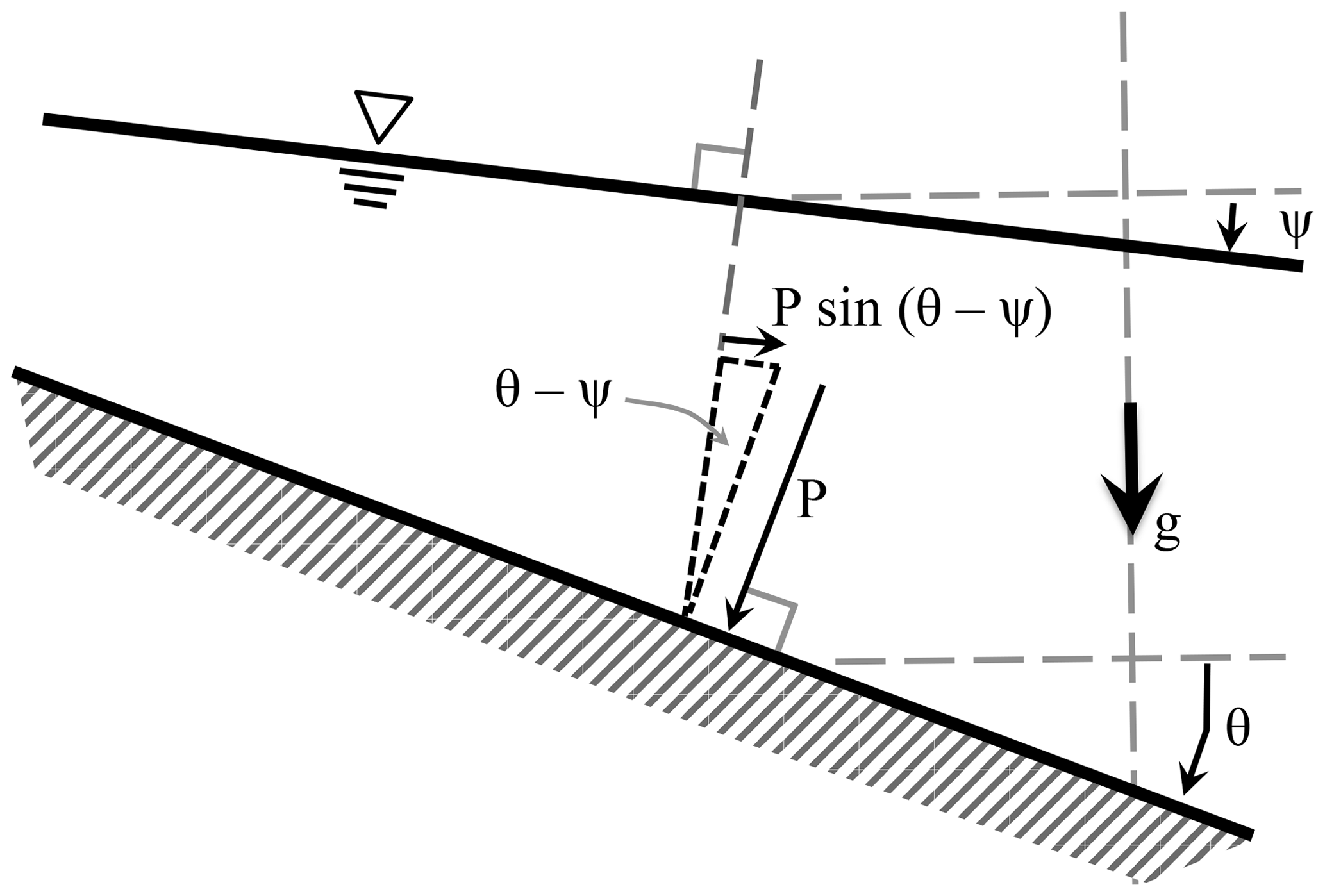
The third pressure term in Eq. (21) is more challenging than the pressure on the flow faces as the bottom surface normal (nk) varies with irregular topography. Hence, the local piezometric pressure contribution in the streamwise direction () at any position (x, y) depends not only on the local water surface elevation but on the local irregularities in topography. It follows that integrating this term over a control volume requires some approximation of the subgrid topography. To arrive at a simpler formulation we note that the pressure acting normal to an arbitrary topography element at position (x, y) with surface normal nk will have force components that can be resolved along a set of local Cartesian axes. One axis is taken along a topography slope angle of θ that lies in the same vertical plane as the streamwise direction , as illustrated in Fig. 2. We can imagine Fig. 2 as an infinitesimal slice across a channel of irregular topography such that a series of these slices (with different θ) can represent any cross-section shape. The second local Cartesian axis is taken within the same vertical plane but perpendicular to the axis defined by θ. The third axis, perpendicular to the other two, is necessarily horizontal and in the cross-channel direction (out of the page in Fig. 2). We are interested only in how the topography contributes to pressure in the streamwise direction, so by definition the cross-channel pressure component is irrelevant. This approach is entirely consistent with changes in depth across the channel and changes in breadth along the channel – both merely alter the surface normal vector nk that is resolved into the local Cartesian system based on the local slope direction of θ.
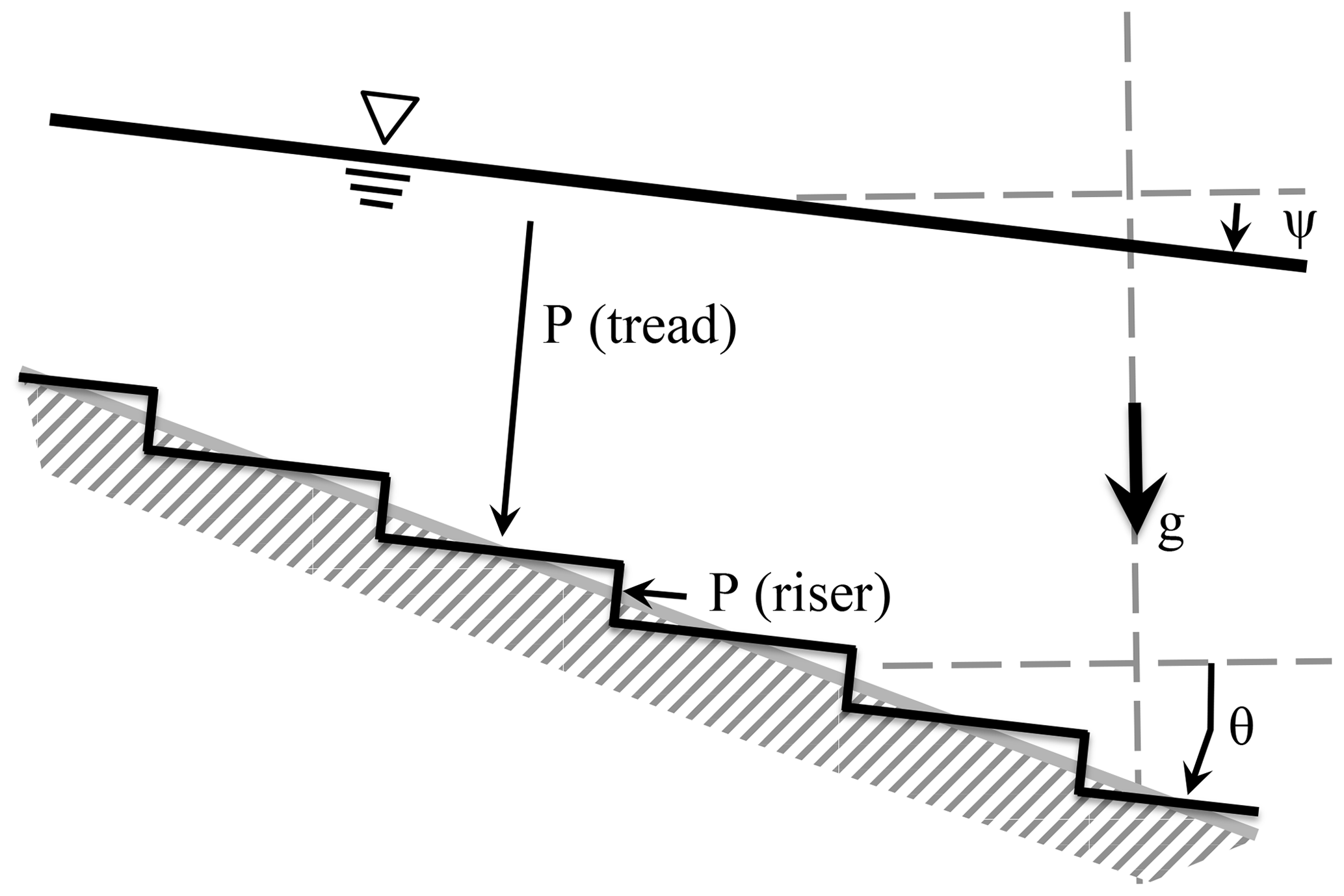
Figure 3Stair-step approximation for pressure along the bottom where tread is parallel to the free surface and riser is perpendicular for linear slopes of both the bottom and free surface.
To isolate the pressure forces acting in the streamwise direction, as a conceptual model we can imagine the topography in the infinitesimal slice of Fig. 2 replaced with a set of m=1 … N stair steps, where the treads are locally parallel to the free surface and the risers are normal to the free surface, as illustrated in Fig. 3. Clearly, as N→∞ we will recover a continuous approximation so there is no need to actually consider the discrete stair steps in a solution method – the steps are merely to illustrate what is otherwise a mathematical abstraction in vector calculus. As illustrated in Fig. 4, we can imagine the stair-step risers as thin planar strips across the entire wetted perimeter that provide a discrete representation of the irregular channel cross-section structure. The only requirements for this conceptual model are that the free surface at longitudinal position x is uniform over the cross section and the slope is aligned with . This conceptual model could also be envisioned in 3-D as discrete rectilinear bricks that approximate the topography: the upper surface of the brick is always aligned parallel with the free surface, the side face is across the channel, and only the front (or back) face is perpendicular to and contributes a topographic pressure force in the streamwise direction. As the brick dimensions go to zero the continuous topography is obtained.
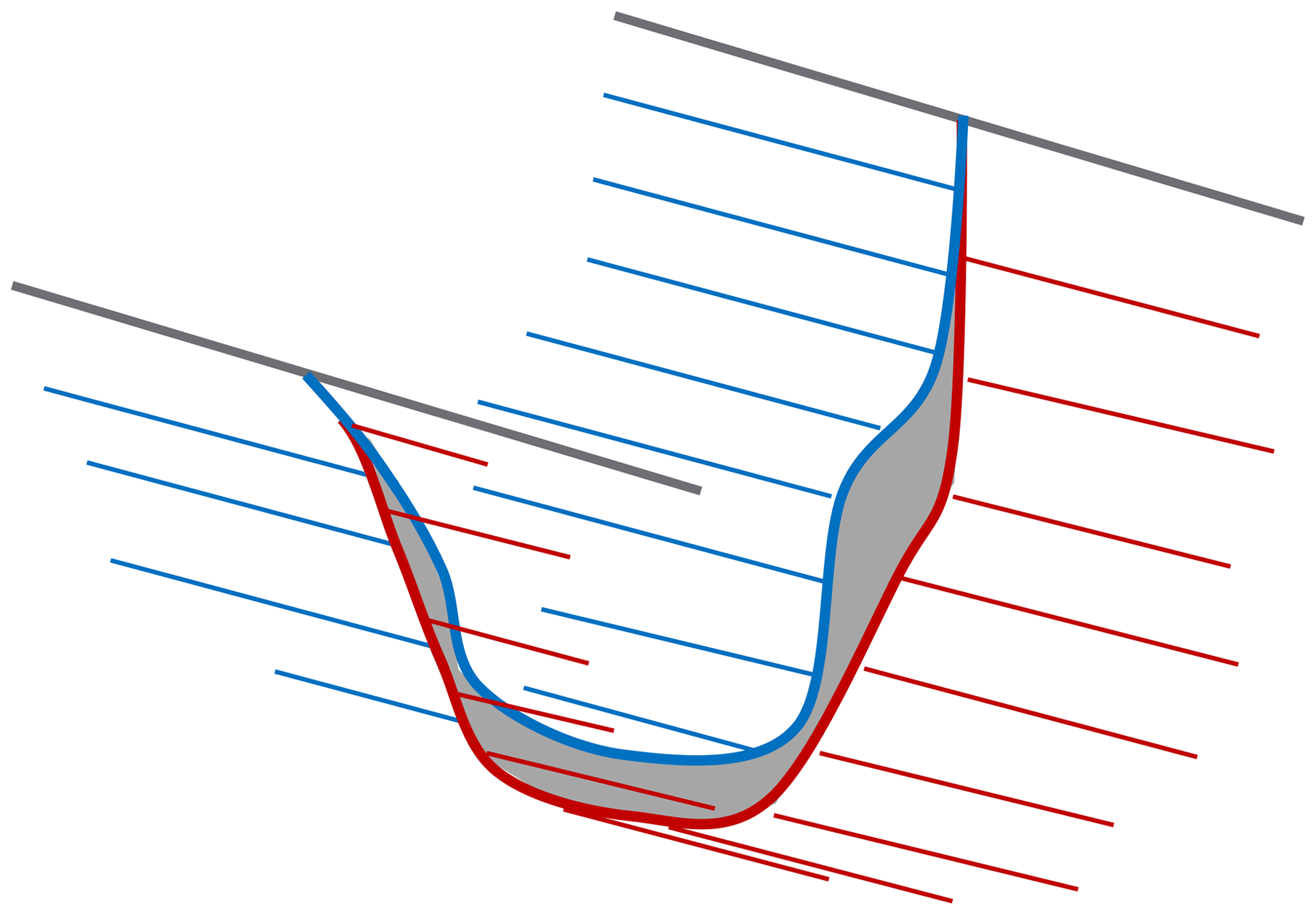
Figure 4Three-dimensional conceptual model of stair-step riser (gray) as a 2-D planar area of AR(m) separating two tread areas (blue, red).
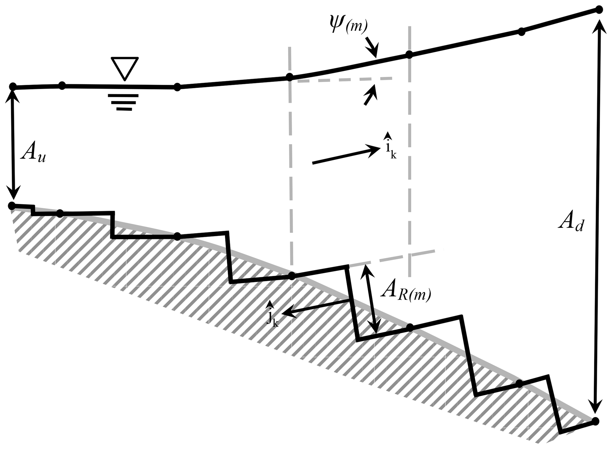
Figure 5Conceptual model of piecewise linear approximation of nonlinear free surface and stair-step approximation of nonlinear topography with the cross-sectional area monotonically increasing. Pressure on the discrete riser area AR(m) is locally aligned with the free-surface slope directly above. The vertical scale and thus the tilt of AR(m) are exaggerated for illustrative purposes.
Since the stair-step treads are (by definition) normal to the modified pressure above, it follows that the only pressure contributions to the momentum in the streamwise direction are on the risers, with individual areas AR(m) for m=1 … N stair steps. Because the pressure contribution for increasing cross-sectional area (i.e., steps down as in Fig. 3) will be opposite of the pressure contribution for decreasing cross-sectional area (i.e., steps upward), it is convenient to introduce a function to account for the change in sign needed for the direction of the pressure force. We can formally define at step m where is the normal unit vector (pointing outwards) from the AR(m) riser, as shown in Figs. 5 and 6 for two different nonlinear water surface profiles over identical bottom topography. It follows that
The above summation can be written as an integral over the length L of the finite-volume element as N→∞.
where is the continuous counterpart to the discrete γ(m). Note that this conceptual model is valid even for non-monotonic behavior of the riser area (e.g., Fig. 6) as long as the AR(m)'s are continuous and smooth as N→∞. However as discussed in Sect. 5, below, extremes of non-monotonic behavior can make it difficult to create a consistent discrete equation for the topographic pressure for a control volume of finite size.
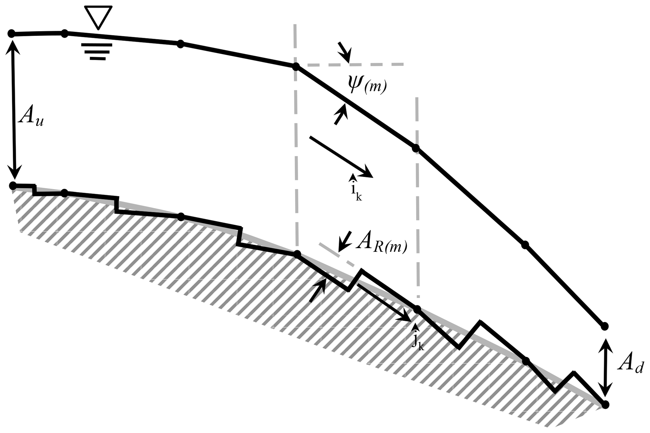
Figure 6Conceptual model of piecewise linear approximation of nonlinear free surface and stair-step approximation of nonlinear bottom with cross-sectional area increasing from Au to the center and then decreasing from the center to Ad. Pressure on the discrete riser area AR(m) is locally aligned with the free-surface slope directly above. The vertical scale and thus the tilt of AR(m) are exaggerated for illustrative purposes. Note that the topography is identical to Fig. 5 but the stair steps are different due to the alteration of the free surface.
For further simplification, it is convenient to introduce the piezometric/non-hydrostatic splitting of Eq. (22) where, by definition, the piezometric pressure is uniform over a vertical cross section (e.g., a stair-step riser). Let P(m) represent the piezometric pressure at the m stair-step riser with area AR(m) so that over a control volume for steps m=1 … N. It follows that
where the continuous AR(x) represents the effective bottom area contributing to the piezometric pressure force in the streamwise direction. Applying this continuous AR(x) form and the hydrostatic/non-hydrostatic splitting to Eq. (29), we obtain
which is a complete representation of the topographic pressure contribution to streamwise momentum in terms of the effective riser areas – i.e., the contribution based on the component of the bottom normal projected in the streamwise direction.
The stair-step conceptual model and AR allow us to consider the pressure effects along the direction due to the changing cross-sectional area of the channel without introducing the separate force terms I1 and I2 of the Cunge–Liggett form of the SVEs. An interesting part of this model is that AR(x) over a control volume is a function of both the local bottom topography and the local free-surface slope. That is, comparing Figs. 5 and 6 we see that AR(m) riser areas are different, despite the identical bottom topography. Returning to our idea that 3-D topography can be represented by discrete bricks, we can imagine each brick is pinned on an axis that allows it to locally rotate to different angles so that the upper surface is always parallel to the free surface. Again, the continuous topography is recovered as the brick size goes to zero, but the brick rotation allows the representation of the different topography effects that are caused by the interaction between the change in relationship between the downstream vector, , and the bottom normal vector as the free-surface profile evolves. Thus, AR is a dynamic representation of the interaction between the free-surface gradient and bottom topography that controls the effective along-stream pressure gradient of converging or diverging flow areas.
In theory, we might directly compute ∫PARdx over a control volume; however, it seems likely that direct discretization of subgrid topography could cause unbalanced momentum source terms. In effect, computing ∫PARdx has the same complexity as computing the I1 or I2 terms of the Cunge–Liggett form and gains us little. Thus, it is useful to consider limiting approximations that can be developed from examining the geometry of Figs. 3 and 5. In the simplest case where both the free surface and bottom have linear slopes (Fig. 3), geometry for the infinitesimal slice requires that
where Adcos ψ represents the cross-sectional area normal to the free surface at the downstream cross section and there is only one value of ψ over the control volume for the linear free-surface slope. Note that the above is an identity for any discrete N stair steps for the linear case. The geometry is somewhat more complex for the nonlinear system of Fig. 5, but the m stair step with free-surface angle ψ(m) must satisfy a similar geometric identity:
where represents the areas normal to the free surface on the upstream and downstream edges of the m piecewise linear stair step. For the nonlinear free surface and/or topography over adjacent linear stair steps there is a discontinuity of the treads for adjacent steps as , so the discrete summation of the stair-step areas over a control volume provides an approximation rather than an identity:
However, in the limit as N→∞ we have a single value of cos ψ at any point along a smooth free surface so that the continuous form provides an identity:
To generalize the above for Ad<Au, we can use the that was introduced for the pressure direction in Eq. (29). Values of indicate that the cross-section area is increasing across location x in the streamwise direction (as in Figs. 3 and 5), whereas indicates that the cross-sectional area is decreasing (as in the latter portion of Fig. 6). It follows that
is an identity that should be satisfied for any control volume where the bottom topography and free surface are continuous and smooth. Note that if Fig. 3 is imagined as one of many infinitesimal slices (with varying θ) that make up a channel cross section, it should be obvious that Eq. (36) also applies for a finite volume with irregular (smooth) topography.
To handle the integration of AR(x) in the piezometric pressure term of Eq. (31), we introduce a quadrature function λ(x), defined as
Note that with Eq. (36), this implies the identity
Using the above in the first term on the RHS of Eq. (31), we obtain
Thus, the introduction of λ allows us to extract a multiplier from the control-volume integral of the bottom pressure. As a result, λ(x) is merely a distribution, or weighting function, for integration of P(x). The full bottom pressure term, Eq. (31), can be written as
Note that λ weighting cannot be readily applied to the non-hydrostatic term because the non-hydrostatic pressure on the bottom has spatial distributions in both the vertical and cross-channel directions that cannot be assumed to be negligible; hence we cannot pass through the AR integration as was done in Eq. (30) for P.
We can think of λ(x) as a weighting function of the conceptual stair-step riser areas over the control-volume length, which controls where the piezometric pressure gradients have their greatest effect. For example, in Fig. 3 the stair-step risers are uniformly distributed such that we can use , which meets the identity requirement of Eq. (38). In contrast, Fig. 5 implies that λ(x) is perhaps a quadratic function. Figure 6 presents a challenge as λ(x) should reverse in sign between the upstream and downstream faces. A key point in the new finite-volume derivation is that λ(x) controls the representation of the free surface and bottom topography within a volume. This can be contrasted to the Godunov approach that uses piecewise linear approximations for both the bottom and free-surface elevations (see Sect. 3). Several discrete approaches to the approximation of λ(x) are examined in Sect. 5, although the full consequences and utility of the λ approach will require more extensive investigation for both theoretical limitations and practical discretization schemes.
4.8 Combining pressure terms
In summary, the pressure terms of Eq. (21) can be written using Eqs. (26), (27), and (40), resulting in
where the last three terms are the non-hydrostatic pressure effects that are typically neglected in the SVEs.
4.9 Viscous term
The remaining term in Eq. (16) is the viscous term, which is treated as an empirical function in all but the most highly resolved models of simple systems – note that Decoene et al. (2009) provide a comprehensive and rigorous approach for friction that has not yet been fully considered in SVE models. For the present purposes, we will retain the simple friction slope form with an assumption of uniform behavior over space, i.e.,
where Sf(e) is the average friction slope over the control volume Ve.
4.10 Finite volume for momentum
Putting together the above, Eq. (16) can be written in a finite-volume form as
where Ue is the element velocity in the streamwise direction, Ve is the element volume, and the relationship between U and Q is given by
Note that Q>0 and U>0 imply flow in the nominal downstream direction, whereas Q<0 and U<0 imply flow in the nominal upstream direction. At this point we have introduced only four approximations: (1) uniform-density incompressibility, (2) the effect of channel curvature is either negligible or handled in an empirical viscous term, (3) the cross-channel variability in the free-surface slope is negligible, and (4) a friction-slope model can be used to represent integrated viscous effects over a control volume. In addition we have a geometric restriction that the upstream and downstream control-volume cross sections must be vertical planes that are orthogonal (in the horizontal plane) to the mean flow direction.
For convenience in exposition, for the remainder of this paper we will apply the hydrostatic approximation () along with approximations for the small slope (cos ψ≈1) and uniform cross-section velocity (β≈1). Furthermore, we will limit our focus to flows without lateral momentum sources (Me=0). These simplifications allow us to focus attention on the pressure source term, which is the primary new contribution in this derivation. The resulting simplification of Eq. (43) can be presented with conservative terms on the LHS and source terms on the RHS as
where definition of piezometric pressure, Eq. (23), is used to substitute P=ρgη. A more formal finite-volume integral presentation would be
Equation (45) can be reduced to a differential equation using V=AL as L→0. Dividing through by L and taking the limit as L→0 provides
If we substitute geometric identities and , we see that the above becomes identical to Eq. (8). Thus, our finite-volume derivation is exactly consistent with the commonly used differential SVEs that is posed using S0. However, from Eqs. (45) and (47) we see that the free-surface source term in the differential form, , is related to the more interesting integral source term in the finite-volume form:
This piezometric pressure term can be thought of as the integrated free-surface/topography effects over a control volume of finite size. It is clear that this term collapses to as L→0, but the integral form cannot be readily inferred from the differential form. Through approximations of this integral term we can obtain a variety of different finite-volume forms of the SVEs, as outlined in the following section.
5.1 General form
We are interested in approximate forms of the finite-volume SVEs that arise from discretization choices in the integral pressure source term derived above, so for exposition it is convenient to start from the approximate form in Eq. (45) with Ve=AeLe and Qe=AeUe. These approximations can be readily reversed to provide a more complete equation, but the simple form for further analysis is
where Te is the source term for integrated free-surface/topography pressure effects obtained from the RHS of Eq. (45):
Note that the LHS of Eq. (48) is discretely conservative in that a summation over all elements will cause all the LHS terms to identically vanish except for the and boundary conditions. Thus, the RHS shows the source terms; i.e., the traditional friction term and a term representing nonlinearities in the free surface interacting with topography can create and destroy momentum. The system is inherently well-balanced as discussed in Sect. 3, as long as Te identically balances the spatially integrated piezometric pressure gradient gAdηd−gAuηu for a flat free surface.
Equation (49) admits a wide variety of approximate equations, depending on the form chosen for the quadrature of η(x) and λ(x) over the length of a finite volume. Arguably, a simple finite-volume discrete method will have three values of η that characterize a control volume: ηu, ηe, and ηd, as illustrated in Fig. 1. Different numerical methods can be constructed by using different approximations constructed from these three values. Herein, we cannot exhaustively investigate the variety of options and so will focus on the most obvious candidates, which are polynomials of orders 0 through 2. The zero-order polynomial is an approximation of η(x) as a uniform value over the element length (e.g., as in the Godunov conceptual model, discussed in Sect. 3) – which could be simply represented by η(x)=ηe so that the face values of ηd and ηu are ignored. Note that even this choice has alternate forms – a slightly different scheme could be constructed using , which is also uniform but ignores ηe. A first-order polynomial for η(x) implies a linear free-surface slope across the element, which might be represented by a slope from ηd to ηu. A second-order polynomial implies a quadratic curvature to the free surface that can pass smoothly through ηu, ηe, and ηd. Clearly this idea could be extended to cubic splines by including adjacent control-volume values. Beyond these polynomials there are other options that might be suitable. For example, we could use the three discrete η values to provide piecewise linear slopes from ηu to ηe and ηe to ηd. The open-ended nature of the η(x) discretization should allow future development of a variety of finite-volume forms that can be easily demonstrated to be well-balanced and consistent with the above derivations.
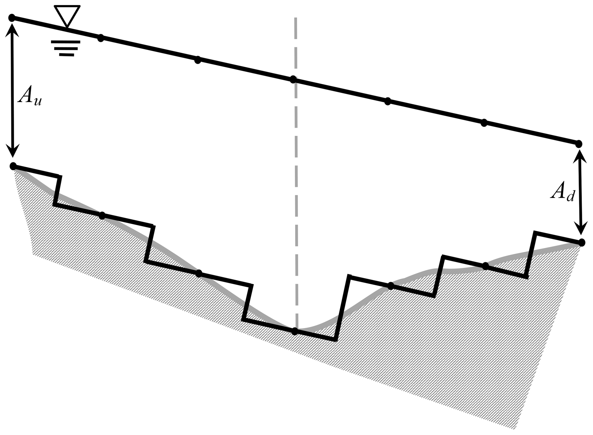
Figure 7Non-monotonic stair steps of the cross-sectional area with linear monotonic free surface. The dashed gray line is where the cross-section area reverses from increasing to decreasing.
By its definition in Eq. (37) with constraint Eq. (38), the weighting function λ(x) is an abstraction of the topographic pressure distribution over a finite volume, which is affected by both topography and the local slope of the free surface, as illustrated in Figs. 3, 5, and 6. The λ(x) is more complicated and abstract than η(x) because the free-surface elevation is approximated as uniform across the channel at any x location, but λ(x) represents the integrated effect of complex 3-D topography, e.g., the AR(m) stair step as illustrated in Fig. 4. The key point is that the λ(x) weighting function has an integral constraint of because the change in the cross-sectional area over the control-volume flux faces, Ad−Au, has already been extracted from the integral of PAR through Eq. (39). A comparison of Figs. 5 and 6 shows that λ(x) is not independent of η(x) and hence arguably should be a moderator between the static topography and the dynamics of the free surface. However, the development of λ(x, t) forms that are dynamically dependent on η(x, t) is beyond the scope of the present work. Herein, we appeal to Occam's razor and note that the simplest λ(x) that satisfies the integral constraint is , where Le is the control-volume length, illustrated in Fig. 1. This choice of λ(x) is a zero-order polynomial implying the stair steps are uniformly distributed over the element, as illustrated in Fig. 3. Clearly, for the nonlinear cases in Figs. 5 and 6, this form of λ(x) is an approximation that reduces the nonlinear interaction between the free surface and the topography. Arguably, this is consistent with a discrete scheme using a single-valued geometry function such as ηe=f(Ve) that neglects the effect of the free-surface slope on the relationship between volume and surface elevation. Note that because the Ad−Au area is already extracted from the integral, using ensures that the Te term is exact at the linear limit and a bounded approximation for nonlinear interactions. That is, with it follows that
Thus, the largest possible value for the Te term is based on the maximum piezometric pressure over the control volume acting on the difference between upstream and downstream areas.
The simple form of is consistent with either increasing cross-sectional area (γ(x)>0 over Le) or decreasing cross-sectional area (γ(x)<0 over Le) but is questionable for a non-monotonic case (e.g., Fig. 6). To examine this issue in more detail, consider the somewhat simpler case of a linear free-surface slope with a cross-sectional area that increases along the streamwise direction in the upper section and decreases in the lower section, as shown in Fig. 7. The approach cannot represent the actual change in cross-section area but instead provides a linear trend between Au and Ad as shown in Fig. 8. In contrast, if the control volume in Fig. 7 were split into two separate volumes at the centerline (i.e., the dashed gray line), then the stair steps of Fig. 7 would be readily represented by the approximation as both control volumes would be monotonic.
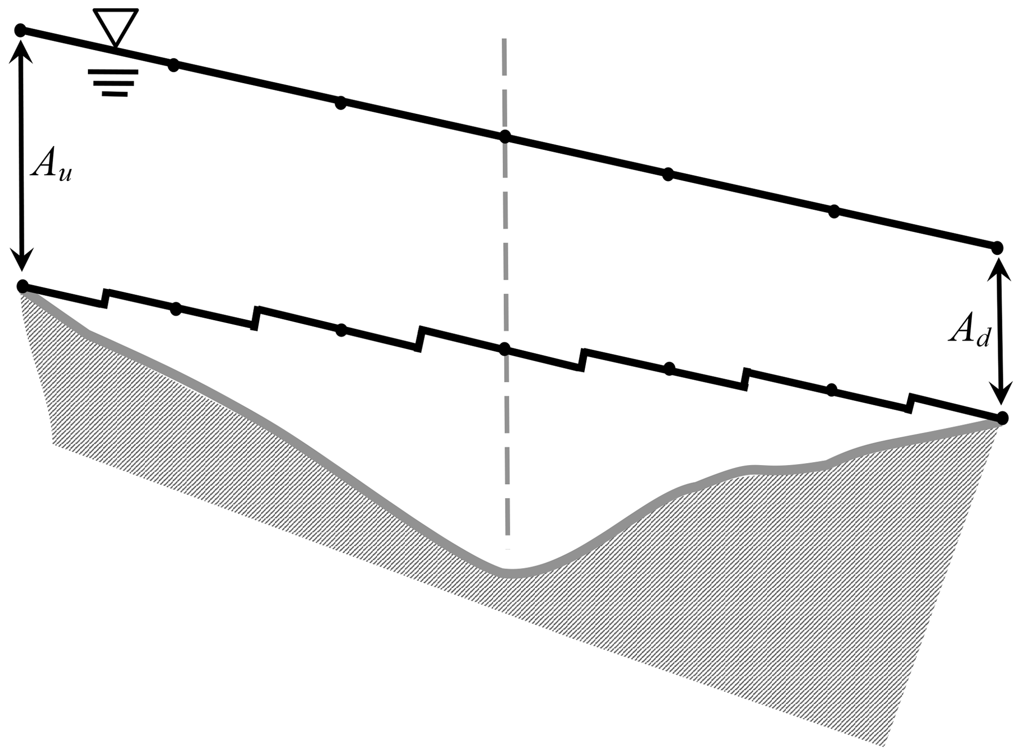
Figure 8Approximated finite-element cross-section characteristics using for non-monotonic topography in Fig. 7. The dashed gray line is where the cross-section area reverses from increasing to decreasing.
A comprehensive investigation of different forms for η(x) and λ(x) in the Te term is clearly needed and will take significant future effort. For the present purposes, we examine the simplest polynomial forms for η(x) in combination with the zeroth-order . To provide insight into how a higher-order λ(x) discretization adds complexity in the derivation, we can derive a simple linear form of λ(x) that depends only on topography and couples with a linear form of η(x). Such a λ(x) is unlikely to be useful with a dynamic free surface but is illustrative of the complexity that can be developed with quadrature of even simple linear equations. We will use the nomenclature Te(m,n) to designate an m-order polynomial for η(x) and an n-order polynomial for λ(x).
5.2 The Te(0,0) approximation
The simplest approximations arise by assuming uniform values such that and , where is the average water surface elevation over the element, and we recall that . It follows that
If we let , then Eq. (48) can be written as
Note that the RHS in the above equation is what we might infer as a discrete finite-volume version of in the differential source term of Eq. (47).
5.3 The Te(1,0) approximation
If we represent the free surface by a first-order polynomial, , while retaining the zeroth-order , we obtain
A linear approximation is consistent with a free surface where b=ηu and , so we obtain a finite-volume source term:
Note that the above implies products of Adηd and Auηu in the source term that can be moved to the LHS as part of the conservative flux terms. Substituting Te(1,0) for Te in Eq. (48) and redistributing terms provides
Thus, the model of a linear free surface and uniform λ(x) serves to change the weighting of the gAη terms (from unity to 1∕2) and provides a source term that contains only face values of A and η, which is unlike Eq. (51) which requires an element approximation of ηe. Interestingly, the above finite-volume form does not have a differential representation as L→0. That is, the free-surface differential source term in Eq. (47) is based on as L→0. However, once we have chosen relationships for η(x) and λ(x) and moved a portion of the source term into the fluxes, an attempt to create a differential out of our source term encounters the form
which can only be reduced to a differential by making additional approximations as to the behavior of A and η at the faces of the finite volume. As a further insight, for the special case of a rectangular channel with frictionless flow Eq. (54) can be transformed by using A=BH, where B is the breadth and H is the depth, so that we obtain a finite-volume form of
As Le→0, and , the above implies a conservative differential form of
which is commonly used in studies of simplified conservative forms (e.g., Bouchut et al., 2003; Hsu and Yeh, 2002). Thus the Te(1,0) is also consistent with prior differential forms.
5.4 The Te(2,0) approximation
We can take this approach further by approximating the free surface as a parabola based on {ηu, ηe, ηd}, where ηe is a characteristic free-surface height at the center of the finite volume. Using with x=0 at Au and x=L at Ad provides
Using results in
It is useful to multiply through and regroup terms so that Adηd and Auηu are isolated. Where these terms are balanced, they can be moved to the LHS as conservative terms. Regrouping provides
So our momentum equation can be written as
Once again, the specific representation of η(x)λ(x) provides a modification of the coefficient of the gAη terms in the conservative fluxes and sets the form of the non-conservative source term. This form does not appear to readily reduce to any differential form that is previously seen in the literature and thus provides an interesting new avenue for investigation.
5.5 The Te(1,1) approximation
The above forms used a uniform . We can readily extend the concept to analytical forms of λ(x), although it is not clear that such increasing complexity will yield an advantage in the design of a numerical model. The λ(x) function is a weighting function that reflects the distribution of the bottom elevation stair steps, as described in Eq. (4). The only restriction on λ(x) is that it must integrate to unity over Le. Physically, as illustrated in Figs. 3, 5, and 6, the λ(x) should be a function of η(x) as well as the topography. However, we do not (as yet) have a good working framework for a dynamic representation of λ(x, η). Thus, to illustrate the complexities that arise with a nonuniform λ(x), herein we will simply analyze a somewhat arbitrary static linear relationship where λ(x)=αz(x), where z is the bottom elevation and α is a scaling constant to ensure . We introduce linear approximations of the bottom as and the free surface as . We can write these approximations as
Using , it can be shown that
Using Eq. (49), a quadrature problem can be presented as
After some algebra, we find
Unfortunately, for the above form we cannot use the redistribution trick to split Te and move a portion to the LHS of Eq. (48). The problem is that any split term will have zu+zd in the denominator, which will not be conservative when used as a coefficient on a control-volume face. Thus, the Te(1,1) form of momentum is
In general, it appears that only the uniform form will allow us to shift part of the source term onto the flux side. Any form that has a nonuniform λ(x) must necessarily have a dependency on z(x) in the cell to satisfy , which creates terms that are inherently non-conservative. Note that this particular Te(1,1) form is for demonstration purposes and is not recommended for use in any numerical scheme. This Te(1,1) is predicated on an assumed weighting of λ(x)=αz(x), which does not have a physical linkage to specific cross-section geometry or expected flow conditions.
5.6 Summary of approximate forms
The Te(0,0), Te(1,0), Te(2,0), and Te(1,1) approximations all follow a similar form
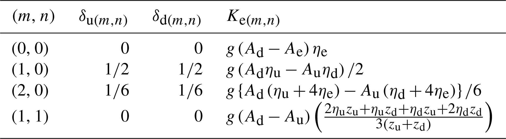
where 0≤δu and δd≤1 are fixed coefficients and Ke(m,n) is a time–space-varying topographic source term, whose exact forms are determined by the approximations used for Te. This form was suggested in Sect. 2 with Eq. (9) based on a philosophical argument of moving as much of the RHS source terms as possible to the conservative LHS flux terms. The key point for future work is that these forms (with the exception of Ke(1,1)) are relatively straightforward in their representation of values that are the natural elements of a SVE computational model for river networks and urban drainage. This approach eliminates the need for estimating or computing the I1 and I2 of the Cunge–Liggett conservative form and replaces them with the simple cross-sectional area term and a Ke that is computed from discrete values of η and A. Values for δu, δd, and Ke for these forms are presented in Table 2. Examination of the above leads to the conclusion that the use of any polynomial representation of η(x) with will produce a Ke(m,0) source term that will exactly balance the piezometric pressure terms of the LHS when the free surface is flat; e.g., . Thus, these schemes are inherently well-balanced as discussed in Sect. 3. Furthermore, for these cases the source terms will be Lipschitz smooth as long as the solution variables are smooth.
Table 2Values for conservative Aη coefficients and Ke(m,n) source terms for finite-volume schemes with (m, n) polynomial approximations of Te. Note that forms using (m, n)=(m, 1) are not recommended without further theoretical development and are provided only for illustrative purposes.
The conservative differential form of the non-hydrostatic version of the Saint-Venant equations, simplified from the derivation in Sect. 4, can be written as
where me is the source and sink of momentum from lateral fluxes per unit length (i.e., MeL−1). This equation is similar to previous work but includes both non-hydrostatic terms and effects of free-surface slope (cos ψ) that are often neglected. The key contribution of the present work is the semi-discrete, conservative, finite-volume form that corresponds to the differential form above:
where and are the average non-hydrostatic pressures on the upstream and downstream cross-sectional areas. In this finite-volume form, the only approximations introduced are listed as follows: (1) uniform-density incompressibility, (2) the effects of momentum redirection around bends is either negligible or is handled in friction terms, (3) the cross-channel variability in the free-surface slope is negligible, and (4) a friction slope model can be used to represent integrated viscous effects. In addition we have introduced a geometric restriction that the upstream and downstream cross sections must be vertical planes that are orthogonal (in the horizontal plane) to the mean flow direction. The above form can be used to analyze systems that include non-hydrostatic pressure and slope gradients beyond the small-slope approximation of the traditional SVEs. As warning for future development of non-hydrostatic methods, note that the fundamental 1-D derivation is effectively treating the non-hydrostatic pressure gradients in the horizontal as absorbing and redirecting momentum along the curving channel. Thus a part of this term is, in effect, encapsulated within the approximation that allows Au and Ad to be cross sections that are not parallel.
The principal feature of the new finite-volume formulation is the topographic source term ∫η(x)λ(x)dx that can be represented by analytical functions to approximate a smoothly varying free surface and its interaction with topography across the finite-volume element. Discrete polynomial representations of ∫η(x)λ(x)dx are evaluated in Sect. 5, with the resulting topographic terms designated as Te(m,n) for an m-degree polynomial representing η and an n-degree polynomial representing λ. In an approximate form, the Te(m,n) term is split into a δu(m,n) factor applied to gAuηu and a δd(m,n) factor applied to gAdηd, which become part of the conservative flux terms. The remainder of the Te(m,n) becomes a Ke(m,n) source term in the approximate finite-volume form. Simpler conservative finite-volume forms that use the common approximations of the hydrostatic equations () with small free-surface slope (cos ψ≈1), uniform cross-sectional velocity (β≈1), and no momentum sources (Me=0) can be written as
where the discrete Ke and δ terms are shown in Table 2. It is worthwhile to compare the above to a finite-volume form derived using the Cunge–Liggett form of the SVEs, which could be written (using the I1 and I2 definitions) as
Performance of the traditional scheme depends on the specification for B(x, z) that defines the irregular bathymetry of the channel. Although the B(x, z) term is developed without any approximations, it is a nontrivial matter to simplify these terms to create practical computational forms for irregular cross-section geometry. The source term on the RHS of the Cunge–Liggett form is effectively an integration of both variations in the channel topography and the water surface elevation over the volume – similar to the new Te – but without a limiting constraint (i.e., is not inherently limited in magnitude for irregular topography). Furthermore, the selection of B(x, z) for the RHS affects the integration on the LHS hydrostatic pressure term – thus obtaining a well-balanced source term that compensates for S0 will also affect the conservative flux terms. The λ(x) used to develop the Ke term Eq. (72) serves a similar purpose to the source-term integral in the Cunge–Liggett form, but it provides a simple weighting function that can be analytically integrated with an approximation for η(x) and is inherently constrained such that over a control volume. The other major difference between the two approaches is that Eq. (73) uses S0 as a source term on the RHS of the equations, whereas in the new approach Eq. (72) dispenses with this artifice so that the source terms only include friction (which is guaranteed to damp momentum) and the portion of the topographic effects that cannot be transferred into the conservative δu and δd terms.
There is a long history of the use of S0 in the source term in the SVEs, and it is indeed part of the author's prior model (Liu and Hodges, 2014). However, the use of S0 with irregular geometry brings the problems of creating a well-balanced conservative scheme, as discussed in Sect. 3. Furthermore, the use of S0 in the source term requires the pressure term to be treated as the hydrostatic pressure rather than the piezometric pressure, as shown in Sect. 4. Because the hydrostatic pressure is a function of depth, its integration over a cross-sectional area requires knowledge of the distribution of depth across the channel – a significant computational complexity for irregular topography. In contrast, the integration of the piezometric pressure over a cross section is exactly PA and does not require knowledge of how depth is distributed across the channel. Other authors have noted similar problems: Schippa and Pavan (2008) derived a conservative differential form that retained gI1 in the flux terms and removed S0 by showing that it could be combined with the I2 source term as for a uniform water level. It seems that the Schippa and Pavan (2008) differential equation might be preferred to the approach proposed herein for high-resolution topography with small grid spacing (i.e., where we have confidence that the computation of I1 is meaningful). However, at larger scales where geometric cross sections are broadly spaced and the computation of I1 is questionable, the simplicity of using A and η for piezometric pressure gradient terms is likely to be preferred. Other authors, notably Rosatti et al. (2011), have simply accepted as an unavoidable source term rather than dealing with the problems of obtaining a well-balanced method with the hydrostatic pressure.
Since S0 was not in de Saint-Venant's original paper, how did it come to be commonly used in the Saint-Venant equations? Arguably there are two sources associated with different simulation scales: (1) in hydrology the kinematic wave model provides S0=Sf, which leads to prioritization of S0 as a hydraulic parameter; and (2) in mathematics the equation
is the canonical form of a 1-D inhomogeneous hyperbolic advection equation for depth h and velocity u, which leads to a prioritization of the depth as a fundamental parameter and requires that S0(x) be relegated to the source term for irregular geometry. However, for solution of the SVEs there is no need to exactly mimic the hyperbolic advection equation to obtain a conservative form; thus there is no need to introduce S0. The above comparisons of the Cunge–Liggett form and the new finite-volume form illustrate the additional complexity of introducing S0. Beyond these issues is a more fundamental problem: numerical methods for inhomogeneous partial differential equations are only well-posed if the source terms are Lipschitz smooth (e.g., Iserles, 1996) – otherwise one should not be surprised by numerical instabilities and/or difficulties in convergence. Any river model that uses raw data from surveyed cross sections will inherently have a non-smooth S0(x). As a result, much of the computational complexity is likely to be compensating for the lack of Lipschitz smoothness in the boundary conditions of topography. In contrast, when the free-surface elevation (piezometric pressure) is used instead of depth (hydrostatic pressure), then S0(x) disappears from the SVEs and the smoothness of the source term is assured (for smooth solution variables) by the choice of smooth functions for λ(x) and η(x) and the friction slope model Sf(x). In general, as long as the solutions of η and Q remain smooth the source term of the SVEs, as derived herein, should remain smooth. That is, the approach herein cannot guarantee a smooth solution, but it can guarantee that any observed non-smoothness in the source terms during a simulation is a result of non-smoothness in the solution variables rather than direct forcing of boundary conditions.
As a matter of pure speculation, the new form of the finite-volume equations brings up some interesting possibilities for large-scale modeling. Imagine that we would like to model a river network or urban drainage network where we have some high-resolution (1×1 m) data in some areas but not in others. Let us also say our computer power limits us to a SVE solution with a median cell length of about 20 m. Can we use our high-resolution knowledge directly at the coarse scale? Arguably, the λ(x) approach could give us a means of directly incorporating effects of subgrid-scale topography into a single source term – however, significant theoretical work is required to develop a consistent methodology that retains the fundamental well-balanced and Lipschitz smooth characteristics of the finite-volume equations.
Clearly, there remains much practical experimentation to be done in comparing various forms of Te(m,n) and the effectiveness of different numerical solution methods with different η(x) polynomial representations. There is also a need to develop a firm theoretical relationship between λ(x) and η(x) to overcome the difficulties illustrated with Figs. 5 and 6 where nonlinear interactions between the free surface and topography cannot be readily represented with the uniform applied herein. Finally, there are substantial questions on whether the new approach can be used with methods designed to satisfy the entropy criterion (e.g., Greenberg and Leroux, 1996; Harten et al., 1983; Lax, 1973). It is hoped that researchers will consider adapting their finite-volume codes to the form of Eq. (72) and reporting their experience.
New finite-volume forms of integral momentum equations for unsteady flow in open channels with varying cross sections are derived in this paper. These equations reduce to the classic differential forms of the Saint-Venant equations (under the Te(0,0) and Te(1,0) approximations) and also provide new approximate finite-volume forms that are suitable for analytical representations of topography and free-surface elevation over a finite-volume element. The new forms use the piezometric pressure (free-surface elevation) rather than hydrostatic pressure (depth) as a fundamental variable and thus do not include the channel slope, S0. This approach provides a cleaner finite-volume form as the nonlinear interactions of topography and the free surface are handled in a single integral term, , where λ is a quadrature weighting function and Ad−Au is the downstream increase in cross-sectional area of the control volume. The introduction of λ(x) provides a potential avenue to convert practical knowledge of fluid and/or geometry variations within a control volume into source and flux terms of the finite-volume equations. The derivations herein can be used to generate a variety of conservative, well-balanced, finite-volume forms for the SVEs that could be employed with a wide range of numerical discretization schemes. This work provides only the theoretical development for the new finite-volume equations; the practical implementation and numerical testing remains a subject for future work.
A demonstration code for discretized application of the new SVE form is available on GitHub at https://github.com/benrhodges/SvePy. This code is associated with a companion paper (Hodges and Liu, 2019) that explains the discretized form.
To elaborate on Eq. (19), the advection of some quantity ϕ through a control volume bounded by surface S can be represented as
where is the local normal velocity across a flux surface. For a flux surface of area A, we define the nonlinearity of distribution across the surface as
where Φ is the average of ϕ over flux area A, and is the average surface normal velocity. Note that because and are derived from projection of the velocity onto the surface normal vector, they have positive signs for outflows and negative sign for inflows. Consistency of and ensures that α≥0; however, this introduces a nomenclature difficulty because the sign does not depend solely on the nominal upstream or downstream direction of the flow. To simplify the nomenclature, we consider only upstream (u) and downstream (d) flux surfaces for a control volume and represent the normal velocity by U⟂ such that a downstream velocity on any face is and an upstream velocity on any face is . It follows that
where
Let with the same sign conventions as U⟂, so that
Consider a channel with a linear free surface so that a velocity parallel to the free surface () has the same direction over the entire control volume. Let and so we obtain
where is interpreted as the average velocity parallel to the free surface with the same sign conventions as U⟂. For a free surface at angle ψ from the horizontal it follows that
Using Eq. (A4) with and provides
Noting that we obtain
Thus, α of Eq. (A4) for is identical to β of Eq. (18). It follows that
which is Eq. (19). However, because it follows that . Thus, equivalent forms are
which all reduce to conventional forms with Q=UA when cos ψ=1.
The author declares that he has no conflicts of interest.
This article was developed under cooperative agreement no. 83595001 awarded
by the US Environmental Protection Agency to the University of Texas at
Austin. It has not been formally reviewed by the EPA. The views expressed in this
document are solely those of the author and do not necessarily reflect those
of the Agency. The EPA does not endorse any products or commercial services
mentioned in this publication. The author appreciates the helpful discussion
with the reviewers that pointed out places where the draft manuscript was
unclear in presenting the conceptual model.
Edited by: Matthew Hipsey
Reviewed by: two anonymous referees
Abbott, M. B. and Ionescu, F.: On The Numerical Computation Of Nearly Horizontal Flows, J. Hydraul. Res., 5, 97–117, https://doi.org/10.1080/00221686709500195, 1967. a
Aricò, C. and Tucciarelli, T.: A marching in space and time (MAST) solver of the shallow water equations. Part I: The 1D model, Adv. Water Resour., 30, 1236–1252, https://doi.org/10.1016/j.advwatres.2006.11.003, 2007. a
Audusse, E., Bouchut, F., Bristeau, M.-O., Klein, R., and Perthame, B.: A Fast and Stable Well-Balanced Scheme with Hydrostatic Reconstruction for Shallow Water Flows, SIAM J. Scient. Comput., 25, 2050–2065, https://doi.org/10.1137/S1064827503431090, 2004. a, b
Audusse, E., Bouchut, F., Bristeau, M.-O., and Sainte-Marie, J.: Kinetic Entropy Inequality and Hydrostatic Reconstruction Scheme for the Saint-Venant System, Math. Comput., 85, 2815–2837, https://doi.org/10.1090/mcom/3099, 2016. a
Blanckaert, K. and Graf, W.: Momentum transport in sharp open-channel bends, J. Hydraul. Eng.-ASCE, 130, 186–198, https://doi.org/10.1061/(ASCE)0733-9429(2004)130:3(186), 2004. a
Bollermann, A., Chen, G., Kurganov, A., and Noelle, S.: A Well-Balanced Reconstruction of Wet/Dry Fronts for the Shallow Water Equations, J. Scient. Comput., 56, 267–290, https://doi.org/10.1007/s10915-012-9677-5, 2013. a, b
Bouchut, F. and Morales de Luna, T.: A Subsonic-Well-Balanced Reconstruction Scheme For Shallow Water Flows, SIAM J. Numer. Anal., 48, 1733–1758, https://doi.org/10.1137/090758416, 2010. a
Bouchut, F., Mangeney-Castelnau, A., Perthame, B., and Vilotte, J.: A new model of Saint Venant and Savage–Hutter type for gravity driven shallow water flows, Comptes Rendus Mathematique, 336, 531–536, https://doi.org/10.1016/S1631-073X(03)00117-1, 2003. a
Brunner, G. W.: HEC-RAS River Analysis System Hydraulic Reference Manual, US Army Corps of Engineers, Davis, CA, USA, 2010. a
Buntina, M. V. and Ostapenko, V. V.: TVD Scheme for Computing Open Channel Wave Flows, Comput. Math. Math. Phys., 48, 2241–2253, https://doi.org/10.1134/S0965542508120130, 2008. a
Burger, G., Sitzenfrei, R., Kleidorfer, M., and Rauch, W.: Parallel flow routing in SWMM 5, Environ. Model. Softw., 53, 27–34, https://doi.org/10.1016/j.envsoft.2013.11.002, 2014. a
Canelon, D. J.: Pivoting Strategies in the Solution of the Saint-Venant Equations, J. Irrig. Drain. Eng.-ASCE, 135, 96–101, 2009. a
Casas, A., Lane, S. N., Yu, D., and Benito, G.: A method for parameterising roughness and topographic sub-grid scale effects in hydraulic modelling from LiDAR data, Hydrol. Earth Syst. Sci., 14, 1567–1579, https://doi.org/10.5194/hess-14-1567-2010, 2010. a
Castellarin, A., Di Baldassarre, G., Bates, P. D., and Brath, A.: Optimal Cross-Sectional Spacing in Preissmann Scheme 1D Hydrodynamic Models, J. Hydraul. Eng.-ASCE, 135, 96–105, https://doi.org/10.1061/(ASCE)0733-9429(2009)135:2(96), 2009. a, b
Castro Diaz, M. J., Chacon Rebollo, T., Fernandez-Nieto, E. D., and Pares, C.: On well-balanced finite volume methods for nonconservative nonhomogeneous hyperbolic systems, SIAM J. Scient. Comput., 29, 1093–1126, https://doi.org/10.1137/040607642, 2007. a
Catella, M., Paris, E., and Solari, L.: Conservative scheme for numerical modeling of flow in natural geometry, J. Hydraul. Eng.-ASCE, 134, 736–748, https://doi.org/10.1061/(ASCE)0733-9429(2008)134:6(736), 2008. a, b
Chau, K. W. and Lee, J. H.: Mathematical modelling of Shing Mun River network, Adv. Water Resour., 14, 106–112, 1991. a
Chen, A., Hsu, M., Chen, T., and Chang, T.: An integrated inundation model for highly developed urban areas, Water Sci. Technol., 51, 221–229, 2005. a
Cohen, S., Praskievicz, S., and Maidment, D. R.: Featured Collection Introduction: National Water Model, J. Am. Water Resour. Assoc., 54, 767–769, https://doi.org/10.1111/1752-1688.12664, 2018. a
Crnković, B., Crnjarić-Zic, N., and Kranjcevic, L.: Improvements of semi-implicit schemes for hyperbolic balance laws applied on open channel flow equations, Comput. Math. Appl., 58, 292–309, https://doi.org/10.1016/j.camwa.2009.04.004, 2009. a
Cunge, J. A., Holly, F. M., and Verwey, A.: Practical Aspects of Computational River Hydraulics, Pitman Publishing Ltd, Boston, MA, 1980. a
David, C. H., Habets, F., Maidment, D. R., and Yang, Z. L.: RAPID applied to the SIM-France model, Hydrol. Process., 25, 3412–3425, https://doi.org/10.1002/hyp.8070, 2011. a
David, C. H., Yang, Z.-L., and Hong, S.: Regional-scale river flow modeling using off-the-shelf runoff products, thousands of mapped rivers and hundreds of stream flow gauges, Environ. Model. Softw., 42, 116–132, 2013. a
Decoene, A., Bonaventura, L., Miglio, E., and Saleri, F.: Asymptotic derivation of the section-averaged shallow water equations for natural river hydraulics, Math. Models Meth. Appl. Sci., 19, 387–417, 2009. a
Delis, A. I. and Skeels, C. P.: TVD Schemes for Open Channel Flow, Int. J. Numer. Meth. Fluids, 26, 791–809, 1998. a
Delis, A. I., Skeels, C. P., and Ryrie, S. C.: Implicit high-resolution methods for modelling one-dimensional open channel flow, J. Hydraul. Res., 38, 369–382, 2000a. a
Delis, A. T., Skeels, C. P., and Ryrie, S. C.: Evaluation of some approximate Riemann solvers for transient open channel flows, J. Hydraul. Res., 38, 217–231, https://doi.org/10.1080/00221680009498339, 2000b. a
de Saint-Venant, A. B.: Théorie du mouvement non permanent des eaux, avec application aux crues des rivières et à introduction des marées dans leurs lits, Comptes Rendus des Séances de l'Académie des Sciences, 73, 237–240, 1871. a
Ferreira, V., de Queiroz, R., Lima, G., Cuenca, R., Oishi, C., Azevedo, J., and McKee, S.: A bounded upwinding scheme for computing convection-dominated transport problems, Comput. Fluids, 57, 208–224, https://doi.org/10.1016/j.compfluid.2011.12.021, 2012. a
Gasiorowski, D.: Balance errors generated by numerical diffusion in the solution of non-linear open channel flow equations, J. Hydrol., 476, 384–394, https://doi.org/10.1016/j.jhydrol.2012.11.008, 2013. a
Getirana, A., Peters-Lidard, C., Rodell, M., and Bates, P. D.: Trade-off between cost and accuracy in large-scale surface water dynamic modeling, Water Resour. Res., 53, 4942–4955, 2017. a
Godunov, S. K.: A difference method for numerical calculation of discontinuous solutions of the equations of hydrodynamics, Mathematicheskii Sbornik, 47, 271–306, 1959. a
Gottardi, G. and Venutelli, M.: Central schemes for open-channel flow, Int. J. Numer. Meth. Fluids, 41, 841–861, https://doi.org/10.1002/d.471, 2003. a, b
Goutal, N. and Maurel, F.: A finite volume solver for 1D shallow-water equations applied to an actual river, Int. J. Numer. Meth. Fluids, 38, 1–19, 2002. a
Greenberg, J. M. and Leroux, A. Y.: A well-balanced scheme for the numerical processing of source terms in hyperbolic equations, SIAM J. Numer. Anal., 33, 1–16, 1996. a, b, c
Guinot, V.: Upwind finite volume solution of sensitivity equations for hyperbolic systems of conservation laws with discontinuous solutions, Comput. Fluids, 38, 1697–1709, https://doi.org/10.1016/j.compfluid.2009.03.002, 2009. a, b
Gulbaz, S. and Kazezyilmaz-Alhan, C. M.: Calibrated Hydrodynamic Model for Sazlidere Watershed in Istanbul and Investigation of Urbanization Effects, J. Hydrol. Eng., 18, 75–84, https://doi.org/10.1061/(ASCE)HE.1943-5584.0000600, 2013. a
Harten, A., Lax, P. D., and Van Leer, B.: On upstream differencing and Godunov-type schemes for hyperbolic conservation laws, SIAM Rev., 25, 35–61, 1983. a, b
Hernandez-Duenas, G. and Beljadid, A.: A central-upwind scheme with artificial viscosity for shallow-water flows in channels, Adv. Water Resour., 96, 323–338, https://doi.org/10.1016/j.advwatres.2016.07.021, 2016. a
Hodges, B. R.: Challenges in Continental River Dynamics, Environ. Model. Softw., 50, 16–20, 2013. a, b, c
Hodges, B. R. and Imberger, J.: Simple curvilinear method for numerical methods of open channels, J. Hydraul. Eng.-ASCE, 127, 949–958, https://doi.org/10.1061/(ASCE)0733-9429(2001)127:11(949), 2001. a
Hodges, B. R. and Liu, F.: Rivers and Electric Networks: Crossing Disciplines in Modeling and Simulation, Foundat. Trends Electron. Design Automat., 8, 1–116, 2014. a
Hodges, B. R. and Liu, F.: No-neighbor discretization of a Saint-Venant model for unsteady open-channel flow, J. Hydraul. Res., submitted, 2019. a
Hsu, C.-T. and Yeh, K.-C.: Iterative explicit simulation of 1D surges and dam-break flows, Int. J. Numer. Meth. Fluids, 38, 647–675, https://doi.org/10.1002/fld.236, 2002. a
Hsu, M., Chen, S., and Chang, T.: Inundation simulation for urban drainage basin with storm sewer system, J. Hydrol., 234, 21–37, https://doi.org/10.1016/S0022-1694(00)00237-7, 2000. a
Iserles, A.: A first course in the numerical analysis of differential equations, Cambridge University Press, Cambridge, UK, 1996. a, b
Islam, A., Raghuwanshi, N. S., and Singh, R.: Development and application for irrigation of hydraulic simulation model canal network, J. Irrig. Drain. Eng.-ASCE, 134, 49–59, https://doi.org/10.1061/(ASCE)0733-9437(2008)134:1(49), 2008. a
Ivanova, K., Gavrilyuk, S. L., and Richard, G.: Formation and coarsening of roll-waves in shear shallow water flows down an inclined rectangular channel, Comput. Fluids, 159, 189–203, https://doi.org/10.1016/j.compfluid.2017.10.004, 2017. a, b
Karelsky, K., Papkov, V., Petrosyan, A., and Tsygankov, D.: Particular solutions of shallow-water equations over a non-flat surface, Phys. Lett. A, 271, 341–348, https://doi.org/10.1016/S0375-9601(00)00378-9, 2000. a
Katsaounis, T., Perthame, B., and Simeoni, C.: Upwinding Sources at Interfaces in Conservation Laws, Appl. Math. Lett., 17, 309–316, https://doi.org/10.1016/S0893-9659(04)00012-6, 2004. a
Kesserwani, G., Ghostine, R., Vazquez, J., Ghenaim, A., and Mose, R.: Application of a second-order Runge–Kutta discontinuous Galerkin scheme for the shallow water equations with source terms, Int. J. Numer. Meth. Fluids, 56, 805–821, https://doi.org/10.1002/fld.1550, 2008. a
Kesserwani, G., Mose, R., Vazquez, J., and Ghenaim, A.: A practical implementation of high-order RKDG models for the 1D open-channel flow equations, Int. J. Numer. Meth. Fluids, 59, 1389–1409, 2009. a, b
Kesserwani, G., Liang, Q., Vazquez, J., and Mose, R.: Well-balancing issues related to the RKDG2 scheme for the shallow water equations, Int. J. Numer. Meth. Fluids, 62, 428–448, https://doi.org/10.1002/fld.2027, 2010. a, b
Krebs, G., Kokkonen, T., Valtanen, M., Koivusalo, H., and Setala, H.: A high resolution application of a stormwater management model (SWMM) using genetic parameter optimization, Urban Water J., 10, 394–410, https://doi.org/10.1080/1573062X.2012.739631, 2013. a
Kurganov, A. and Petrova, G.: A second-order well-balanced positivity preserving central-upwind scheme for the Saint-Venant system, Commun. Math. Sci., 5, 133–160, 2007. a, b
Lai, C., Baltzer, R. A., and Schaffranek, R. W.: Conservation-form equations of unsteady open-channel flow, J. Hydraul. Res., 40, 567–578, https://doi.org/10.1080/00221680209499901, 2002. a
Lai, W. and Khan, A. A.: Discontinuous Galerkin Method for 1D Shallow Water Flows in Natural Rivers, Eng. Appl. Comput. Fluid Mech., 6, 74–86, 2012. a, b
Lax, P. D.: Hyperbolic Systems of Conservation Laws and the Mathematical Theory of Shock Waves, chap. 1, SIAM, Philadelphia, Pennsylvania, USA, 1–48, https://doi.org/10.1137/1.9781611970562.ch1, 1973. a
Leandro, J. and Martins, R.: A methodology for linking 2D overland flow models with the sewer network model SWMM 5.1 based on dynamic link libraries, Water Sci. Technol., 73, 3017–3026, https://doi.org/10.2166/wst.2016.171, 2016. a
Li, J. and Chen, G.: The generalized Riemann problem method for the shallow water equations with bottom topography, Int. J. Numer. Meth. Eng., 65, 834–862, https://doi.org/10.1002/nme.1471, 2006. a
Li, M., Guyenne, P., Li, F., and Xu, L.: A Positivity-Preserving Well-Balanced Central Discontinuous Galerkin Method for the Nonlinear Shallow Water Equations, J. Scien. Comput., 71, 994–1034, https://doi.org/10.1007/s10915-016-0329-z, 2017. a
Liang, Q. and Marche, F.: Numerical resolution of well-balanced shallow water equations with complex source terms, Adv. Water Resour., 32, 873–884, https://doi.org/10.1016/j.advwatres.2009.02.010, 2009. a, b
Liggett, J. A.: Unsteady Flow in Open Channels, in: chap. 2: Basic equations of unsteady flow, Water Resources Publications, Fort Collins, Colorado, 1975. a
Liu, F. and Hodges, B. R.: Applying microprocessor analysis methods to river network modeling, Environ. Model. Softw., 52, 234–252, https://doi.org/10.1016/j.envsoft.2013.09.013, 2014. a, b, c, d, e, f, g, h
Lyn, D. A. and Altinakar, M.: St. Venant–Exner Equations for Near-Critical and Transcritical Flows, J. Hydraul. Eng.-ASCE, 128, 579–587, https://doi.org/10.1061/(ASCE)0733-9429(2002)128:6(579), 2002. a
Mohamed, K.: A finite volume method for numerical simulation of shallow water models with porosity, Comput. Fluids, 104, 9–19, https://doi.org/10.1016/j.compfluid.2014.07.020, 2014. a
Monthe, L., Benkhaldoun, F., and Elmahi, I.: Positivity preserving finite volume Roe schemes for transport-diffusion equations, Comput. Meth. Appl. Mech. Eng., 178, 215–232, https://doi.org/10.1016/S0045-7825(99)00015-8, 1999. a
Paiva, R. C. D., Collischonn, W., and Tucci, C. E. M.: Large scale hydrologic and hydrodynamic modeling using limited data and a GIS based approach, J. Hydrol., 406, 170–181, https://doi.org/10.1016/j.jhydrol.2011.06.007, 2011. a
Paiva, R. C. D., Collischonn, W., and Costa Buarque, D.: Validation of a full hydrodynamic model for large-scale hydrologic modelling in the Amazon, Hydrol. Process., 27, 333–346, 2013. a, b
Papanicolaou, A. N., Bdour, A., and Wicklein, E.: One-dimensional hydrodynamic/sediment transport model applicable to steep mountain streams, J. Hydraul. Res., 42, 357–375, 2004. a, b
Paz, A. R., Bravo, J. M., Allasia, D., Collischonn, W., and Tucci, C. E. M.: Large-Scale Hydrodynamic Modeling of a Complex River Network and Floodplains, J. Hydrol. Eng., 15, 152–165, https://doi.org/10.1061/(ASCE)HE.1943-5584.0000162, 2010. a
Perthame, B. and Simeoni, C.: A kinetic scheme for the Saint-Venant system with a source term, CALCOLO, 38, 201–231, https://doi.org/10.1007/s10092-001-8181-3, 2001. a
Pramanik, N., Panda, R. K., and Sen, D.: One dimensional hydrodynamic modeling of river flow using DEM extracted river cross-sections, Water Resour. Manage., 24, 835–852, 2010. a, b
Preissmann, A.: Propagation des intumescences dans les canaux et rivieres, in: Premier Congres De L'Association Francaise de Calcul AFCAL, Grenoble 14–15–16, 1960, Gauthier-Villars, Paris, 433–442, 1961. a, b
Pu, J. H., Cheng, N.-S., Tan, S. K., and Shao, S.: Source term treatment of SWEs using surface gradient upwind method, J. Hydraul. Res., 50, 145–153, https://doi.org/10.1080/00221686.2011.649838, 2012. a, b
Roe, P.: Approximate Riemann solvers, parameter vectors, and difference schemes, J. Comput. Phys., 43, 357–372, https://doi.org/10.1016/0021-9991(81)90128-5, 1981. a
Rosatti, G., Bonaventura, L., Deponti, A., and Garegnani, G.: An accurate and efficient semi-implicit method for section-averaged free-surface flow modelling, Int. J. Numer. Meth. Fluids, 65, 448–473, https://doi.org/10.1002/fld.2191, 2011. a, b
Rossman, L. A.: Storm Water Management Model Reference Manual, in: Volume II – Hydraulics, Tech. Rep. EPA/600/R-17/111, US EPA Office of Research and Development, Water Systems Division, avaialable at: https://nepis.epa.gov/Exe/ZyPDF.cgi?Dockey=P100S9AS.pdf (last access: 5 March 2019), 2017. a, b
Saavedra, I., Lopez, J. L., and García-Martínez, R.: Dynamic Wave Study of Flow in Tidal Channel System of San Juan River, J. Hydraul. Eng.-ASCE, 129, 519–526, https://doi.org/10.1061/(ASCE)0733-9429(2003)129:7(519), 2003. a, b, c
Saleh, F., Ducharne, A., Flipo, N., Oudin, L., and Ledoux, E.: Impact of river bed morphology on discharge and water levels simulated by a 1D Saint–Venant hydraulic model at regional scale, J. Hydrol., 476, 169–177, https://doi.org/10.1016/j.jhydrol.2012.10.027, 2013. a, b
Sanders, B. F.: High-resolution and non-oscillatory solution of the St. Venant equations in non-rectangular and non-prismatic channels, J. Hydraul. Res., 39, 321–330, 2001. a, b, c
Sanders, B. F., Jaffe, D. A., and Chu, A. K.: Discretization of integral equations describing flow in-nonprismatic channels with uneven beds, J. Hydraul. Eng.-ASCE, 129, 235–244, https://doi.org/10.1061/(ASCE)0733-9429(2003)129:3(235), 2003. a, b, c
Sart, C., Baume, J. P., Malaterre, P. O., and Guinot, V.: Adaptation of Preissmann's scheme for transcritical open channel flows, J. Hydraul. Res., 48, 428–440, https://doi.org/10.1080/00221686.2010.491648, 2010. a, b
Schippa, L. and Pavan, S.: Analytical treatment of source terms for complex channel geometry, J. Hydraul. Res., 46, 753–763, https://doi.org/10.3826/jhr.2008.3211, 2008. a, b, c, d, e
Sen, D. J. and Garg, N. K.: Efficient Algorithm for Gradually Varied Flows in Channel Networks, J. Irrig. Drain. Eng.-ASCE, 128, 351–357, https://doi.org/10.1061/(ASCE)0733-9437(2002)128:6(351), 2002. a
Szymkiewicz, R.: Finite-Element Method For The Solution Of The Saint Venant Equations In An Open Channel Network, J. Hydrol., 122, 275–287, https://doi.org/10.1016/0022-1694(91)90182-H, 1991. a
Tucciarelli, T.: A new algorithm for a robust solution of the fully dynamic Saint-Venant equations, J. Hydraul. Res., 41, 239–246, 2003. a
Vazquez-Cendon, M.: Improved treatment of source terms in upwind schemes for the shallow water equations in channels with irregular geometry, J. Comput. Phys., 148, 497–526, 1999. a, b
Venutelli, M.: Stability and accuracy of weighted four-point implicit finite difference schemes for open channel flow, J. Hydraul. Eng.-ASCE, 128, 281–288, https://doi.org/10.1061/(ASCE)0733-9429(2002)128:3(281), 2002. a
Venutelli, M.: A fractional-step Padé Galerkin model for dam-break flow simulation, Appl. Math. Comput., 134, 93–107, 2003. a
Venutelli, M.: A third-order explicit central scheme for open channel flow simulations, J. Hydraul. Res., 44, 402–411, 2006. a, b
Wang, G.-T., Yao, C., Okoren, C., and Chen, S.: 4-Point FDF of Muskingum method based on the complete St Venant equations, J. Hydrol., 324, 339–349, https://doi.org/10.1016/j.jhydrol.2005.10.010, 2006. a
Wang, J., Ni, H., and He, Y.: Finite-difference TVD scheme for computation of dam-break problems, J. Hydraul. Eng.-ASCE, 126, 253–262, https://doi.org/10.1061/(ASCE)0733-9429(2000)126:4(253), 2000. a
Wood, E. F., Roundy, J. K., Troy, T. J., van Beek, L. P. H., Bierkens, M. F. P., Blyth, E., de Roo, A., Doll, P., Ek, M., Famiglietti, J., Gochis, D., van de Giesen, N., Houser, P., Jaffe, P. R., Kollet, S., Lehner, B., Lettenmaier, D. P., Peters-Lidard, C., Sivapalan, M., Sheffield, J., Wade, A., and Whitehead, P.: Hyperresolution global land surface modeling: Meeting a grand challenge for monitoring Earth's terrestrial water, Water Resour. Res., 47, 1–10, 2011. a
Wu, W. M. and Wang, S. S. Y.: One-dimensional Modeling of dam-break flow over movable beds, J. Hydraul. Eng.-ASCE, 133, 48–58, https://doi.org/10.1061/(ASCE)0733-9429(2007)133:1(48), 2007. a, b
Wu, W. M., Vieira, D. A., and Wang, S. S. Y.: One-dimensional numerical model for nonuniform sediment transport under unsteady flows in channel networks, J. Hydraul. Eng.-ASCE, 130, 914–923, https://doi.org/10.1061/(ASCE)0733-9429(2004)130:9(914), 2004. a
Xing, Y.: Exactly well-balanced discontinuous Galerkin methods for the shallow water equations with moving water equilibrium, J. Comput. Phys., 257, 536–553, https://doi.org/10.1016/j.jcp.2013.10.010, 2014. a, b
Xing, Y. and Shu, C.-W.: High-order finite volume WENO schemes for the shallow water equations with dry states, Adv. Water Resour., 34, 1026–1038, https://doi.org/10.1016/j.advwatres.2011.05.008, 2011. a
Xing, Y. and Zhang, X.: Positivity-Preserving Well-Balanced Discontinuous Galerkin Methods for the Shallow Water Equations on Unstructured Triangular Meshes, J. Scient. Comput., 57, 19–41, https://doi.org/10.1007/s10915-013-9695-y, 2013. a
Ying, X. and Wang, S. S. Y.: Improved implementation of the HLL approximate Riemann solver for one-dimensional open channel flows, J. Hydraul. Res., 46, 21–34, 2008. a, b
Ying, X., Khan, A. A., and Wang, S. S. Y.: Upwind Conservative Scheme for the Saint Venant Equations, J. Hydraul. Eng.-ASCE, 130, 977–987, https://doi.org/10.1061/(ASCE)0733-9429(2004)130:10(977), 2004. a, b
Zeng, W. and Beck, M. B.: STAND, a dynamic model for sediment transport and water quality, J. Hydrol., 277, 125–133, https://doi.org/10.1016/S0022-1694(03)00073-8, 2003. a
Zhu, D. J., Chen, Y. C., Wang, Z. Y., and Liu, Z. W.: Simple, Robust, and Efficient Algorithm for Gradually Varied Subcritical Flow Simulation in General Channel Networks, J. Hydraul. Eng.-ASCE, 137, 766–774, https://doi.org/10.1061/(ASCE)HY.1943-7900.0000356, 2011. a