the Creative Commons Attribution 4.0 License.
the Creative Commons Attribution 4.0 License.
 | 11 Mar 2019
Combining continuous spatial and temporal scales for SGD investigations using UAV-based thermal infrared measurements
Christian Siebert
Submarine groundwater discharge (SGD) is highly variable in spatial and temporal terms due to the interplay of several terrestrial and marine processes. While discrete in situ measurements may provide a continuous temporal scale to investigate underlying processes and thus account for temporal heterogeneity, remotely sensed thermal infrared radiation sheds light on the spatial heterogeneity as it provides a continuous spatial scale.
Here we report results of the combination of both the continuous spatial and temporal scales, using the ability of an unmanned aerial vehicle (UAV) to hover above a predefined location, and the continuous recording of thermal radiation of a coastal area at the Dead Sea (Israel). With a flight altitude of 65 m above the water surface resulting in a spatial resolution of 13 cm and a thermal camera (FLIR Tau2) that measures the upwelling long-wave infrared radiation at 4 Hz resolution, we are able to generate a time series of thermal radiation images that allows us to analyse spatio-temporal SGD dynamics.
In turn, focused SGD spots, otherwise camouflaged by strong lateral flow dynamics, are revealed that may not be observed on single thermal radiation images. The spatio-temporal behaviour of an SGD-induced thermal radiation pattern varies in size and over time by up to 155 % for focused SGDs and by up to 600 % for diffuse SGDs due to different underlying flow dynamics. These flow dynamics even display a short-term periodicity of the order of 20 to 78 s for diffuse SGD, which we attribute to an interplay between conduit maturity–geometry and wave set-up.
- Article
(5112 KB) -
Supplement
(96 KB) - BibTeX
- EndNote


Submarine groundwater discharge (SGD) is defined as “any and all flow of water on continental margins from the seabed to the coastal ocean” (Burnett et al., 2003). The definition already implies several proportions of water with different origins contributing to SGD. Apart from recirculated seawater, it is also fresh groundwater of meteoric origin. The relative share of each water contribution depends on terrestrial and marine controls. Recharge amounts, aquifer permeability and hydraulic gradients define the terrestrial groundwater contribution, which may be the major SGD share in areas with high permeability, such as karstic environments. In areas with low hydraulic gradients and low aquifer permeability, recirculated seawater as a share of SGD predominates. The recirculation is induced by the highly variable hydraulic gradients caused by tidal or lunar cycles, storms, or wave set-up. In situ measurements such as seepage meters, multilevel piezometers, tracers, etc. possess the ability to discriminate between the SGD shares and allow a linkage to the underlying processes, since the investigated temporal scale is continuous and ranges between daily and seasonal cycles (Taniguchi et al., 2003a; Michael et al., 2011). Yet, all of this cannot account for the spatial variability, as the entity and interaction of terrestrial and marine controls lead to a highly variable SGD appearance in terms of discharge type (diffuse vs. focused), temporal discharge behaviour, flow rates, spatial abundance (even over small spatial scales), and mixing (Michael et al., 2003; Taniguchi et al., 2003b; Burnett et al., 2006).
In contrast, remote sensing technology allows identification and quantification of SGD over larger spatial scales without neglecting its spatial and temporal variance, or the need to extrapolate from in situ measurements. Depending on the intended spatial scale, utilized platforms differ between satellite (spatial coverage > 10 000 km2), airplane (spatial coverage > 100 km2), and unmanned aerial vehicle (hereafter UAV) systems (spatial coverage > 100 km2). From these systems the majority of all approaches measure thermal infrared radiation (hereafter thermal radiation/radiances) (i.e. Mejías et al., 2012; Kelly et al., 2018; Mallast et al., 2013b; Lee et al., 2016).
The principle of using thermal radiation for SGD detection is based on temperature contrasts between SGD water and ambient water at the sea surface. Since the surface temperatures are directly proportional to emitted thermal radiation (see Stefan–Boltzman law) and assume a rather similar emissivity for water, sea surface temperature contrasts evoke distinguishable thermal radiation patterns or thermal radiation anomalies, which are indicative of SGD. This qualitative approach has been expanded by a few studies that use thermal anomalies to quantify SGD through a relation of anomaly (plume) size to measured or modelled SGD rates (Kelly et al., 2018; Tamborski et al., 2015; Lee et al., 2016). Given a positive buoyancy of less saline groundwater in marine environments, the intriguing simplicity of these approaches is based on the momentum of discharging groundwater (Mallast et al., 2013a) and a potential deflection in the water body due to currents and wave action (Lee et al., 2016), external forces (e.g. wind) (Lewandowski et al., 2013), and Newton's law of cooling (Vollmer, 2009). While the latter leads to a convective heat transfer between the discharging and the ambient water with exponential adaption behaviour at the fringe of the plume, the momentum and deflections are the forces defining the size and shape of the plume. In turn, the momentum leads to a positive relationship between plume size and discharge rate (Johnson et al., 2008; Mallast et al., 2013a; Lee et al., 2016) for parts of the plume not being deflected and demonstrates the practicability and numerous advantages in terms of spatial continuity. The possible quantification approach, however, relies on thermal radiation snapshots recorded at a certain instantaneous time (Kelly et al., 2018; Tamborski et al., 2015).
Thus, in terms of scale, the advantage of remote sensing for SGD investigations is the continuous spatial scale, which allows the derivation of a general picture in regard to SGD abundance and quantity independent of its appearance and spatial variability. On the other hand, the advantage of in situ measurements is explicitly the continuous temporal scale, which permits a process understanding and elaboration on the drivers.
However, with the advent and the ability of multicopters as a type of UAV to hover over a predefined location, it becomes possible to combine the continuous spatial and temporal scales in an unrivalled resolution and to investigate the spatio-temporal behaviour of SGD in one context. Here we report the results of such a study that uses a thermal camera system mounted beneath a multicopter. The multicopter hovers above a predefined location to (i) investigate the spatio-temporal variability of focused and diffuse SGD and (ii) to outline additional values of the presented approach. The study is conducted at a site on the hypersaline Dead Sea, at which previously investigated submarine and terrestrial springs emerge. Existing hydraulic gradients in the discharging aquifers and high density differences between groundwater and lake water qualify the terminology SGD, which is usually bound to marine environments only.
The study was conducted at a known and pre-investigated SGD site (see Sect. 2.2) at the eastern slope of the sedimentary fan of Wadi Darga, located at the western coast of the Dead Sea (Fig. 1a, d, e).
2.1 Hydrogeological setting
Discharging groundwater at the study area is replenished in the Judean Mountains either through precipitation or flash floods that infiltrate into the Upper Cretaceous limestone and dolostone of the Judea Group Aquifer (JGA) and flow east towards the Dead Sea Rift (DSR). After passing the transition to the DSR, which is marked by normal faults and block tectonics, fresh groundwater enters the Quaternary fluvio-lacustrine Dead Sea Group (DSG) that is deposited in front of the Cretaceous rocks (Yechieli et al., 2010). The DSG consists of stratified fine-grained lacustrine sediments (clay minerals, aragonite, gypsum, halite), which are intercalated with coarser clastic layers. At wadi outlets, the lacustrine strata are displaced with fluviatile fine to coarse clastic sediments (Yechieli et al., 1995).
Due to the alternations of coarse and fine strata, groundwater flow occurs through separated subaquifers that possess different groundwater levels (Yechieli et al., 2010). In addition, preferential flow paths in the form of dissolution tubes and cavities develop due to dissolution of the evaporitic minerals (Magal et al., 2010; Ionescu et al., 2012). The dissolution process accelerates with the continuous and fast drop of the Dead Sea water level of ∼ 1 m yr−1 (Yechieli et al., 2010), which forces the formation of new groundwater flow paths. The resulting partially karstic flow system in the DSG is highly transient, resulting in immensely variable discharge rates, discharge locations and chemical composition of springs along the lakeshore (Burg et al., 2016). Besides admixing of interstitial brines to the groundwater, the degree of water–rock interaction in the DSG controls the groundwater's composition. Hence, large observable differences in the composition of discharging groundwater, which occur even within the range of a few metres, are an expression of the heterogeneous maturity of the karst system. The less mature the conduits, the larger the ratio between wetted soluble surfaces and volume.
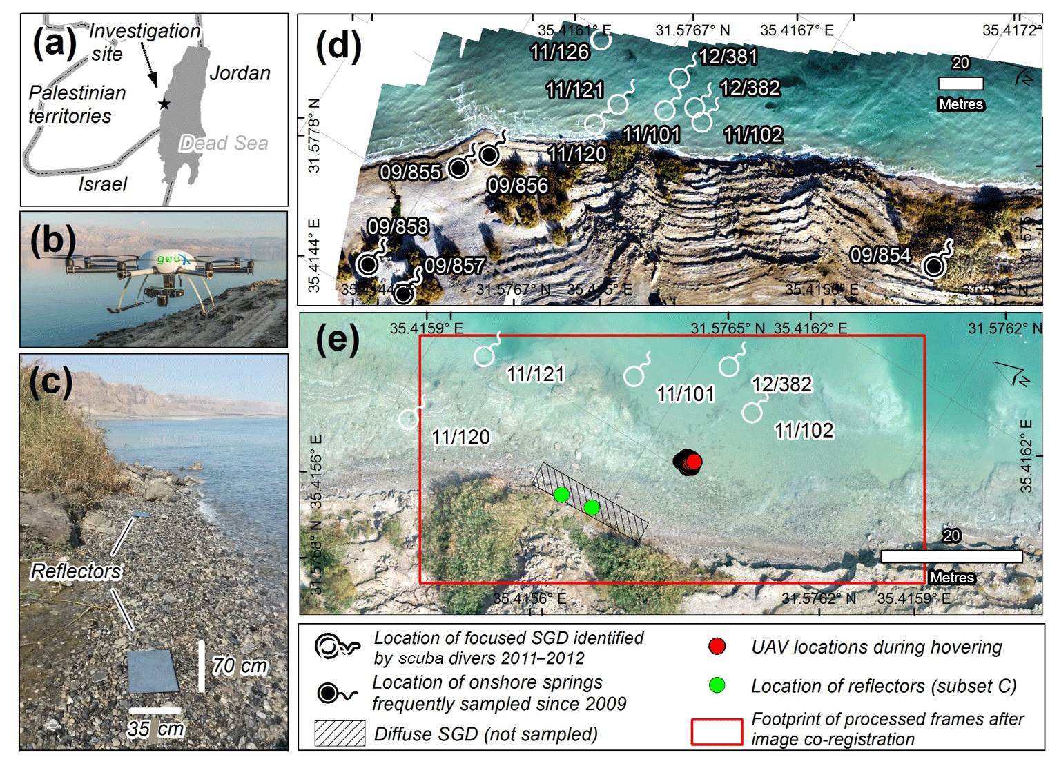
Figure 1Location of the study area at the Dead Sea (a), photo of the UAV used during the study (b), photo of both reflectors at the covered coastline section (c), distribution of focused SGD spots identified and sampled by divers in the years 2011 and 2012, and onshore springs which have been sampled frequently since 2009 (d), and an aerial photograph from 10 February 2016 at 12:11 LT of the covered area along with UAV positions during hovering, location of reflectors, the footprint of the processed frames after co-registration described in Sect. 2.3 and locations of observed diffuse SGD (e).
Consequently, diffuse SGD exhibits a high load of dissolved solids and thus is saline (less mature karst system), while focused SGD is less loaded and exhibits a lower salinity (mature karst system).
2.2 Submarine groundwater discharge and onshore spring characteristics
At the investigation site, focused SGD occurrences were mapped in 2011 and 2012 by scuba divers and hydrochemically investigated. Based on their findings groundwater emerges from mature karst-like cavities down to depths of 30 m below the sea surface (Ionescu et al., 2012; Mallast et al., 2014).
From these cavities groundwater emerges as focused SGD. Subsequently, density differences between SGD water (1.00–1.19 g cm−3) and Dead Sea brine (1.234 g cm−3) trigger a continuous positive buoyancy (buoyant jet) of the emerging groundwater towards the lake's surface. Within the water column and alongside the buoyant jet, considerable turbulences develop, entraining ambient Dead Sea brine. Thus, the ascending water represents a mixture of fresh to brackish groundwater and lake brine. Once the ascending mixture reaches the lake's surface, it develops a radially orientated flow away from its jet centre, causing a circular-like pattern. These patterns are partially visually observable as shown in Mallast et al. (2014) at the Dead Sea and in various other cases (Swarzenski et al., 2001).
Apart from focused SGD, diffuse SGD occurs at the investigation site as well, either in various depths below the water surface (Ionescu et al., 2012) or at the shoreline. At the study area one diffuse SGD site exists directly at the shoreline (Fig. 1e). The discharge seems to occur over a length of approximately 20–25 m alongshore and was only detectable visually through the occurrence of schlieren in the lake brine. However, low discharge rates in combination with the immediate mixing with the lake brine impede any attempt to sample that water.
In order to still be able to compare groundwater characteristics, we sampled five onshore springs (Fig. 1d). All are in close proximity to previously mentioned SGD and to the shoreline, but emerge as focused flow in different elevations of 0.5–10 m above the Dead Sea water level. The water characteristics are shown in Table 2.
2.3 Hydrologic and atmospheric setting
According to on-site measurements, SGD water temperatures at the orifices are 21–31.5 ∘C. During the time of investigation the Dead Sea had a skin temperature of ∼ 21 ∘C providing a temperature maximum difference of 10.5 ∘C between groundwater and ambient Dead Sea brine. Wind speeds amounted to 0.87 m s−1 (±0.16) approaching from SE to E (80–128∘). Occurring waves, which may influence SGD size and shape, had a frequency of 3–7 s with estimated wave heights <15 cm. During the flight, cloud-free conditions and thus homogeneous solar radiation existed, equally reflected at the sea surface throughout the entire covered area.
The general approach to investigate the spatio-temporal thermal radiation variability induced by SGD consists of hovering with an UAV (multicopter – model: geo-X8000) (Fig. 1b) above a pre-defined SGD spot (Fig. 1c) over a time period of several minutes. The flight was conducted on 10 February 2016 between 12:43 and 12:50 LT (local time), with activated image recording between 12:45 to 12:48 LT. During that flight the UAV was equipped with a thermal system comprising (i) a long-wave infrared camera core (FLIR Tau2), which is an uncooled VOx Microbolometer with a 19 mm lens and a 640 × 512 focal plane array (FLIR® Systems 2016) and (ii) a ThermalCapture radiometry module and image grabber (TeAx Technology, 2016). The system senses long-wavelength infrared radiation in the spectral range of 7.5–13.5 µm with a sensitivity of <50 mK. Subsequently, sensed radiation is captured as 14 bit images at a frame rate of 9 Hz, from which only every fifth frame is exportable (approx. 4–5 Hz), deduced after our own tests. The core was calibrated prior to the flight using an internal flat-field corrector.
The hovering position was at 31.576516∘, 35.415775∘ with a flight altitude of 65 m above Dead Sea level. Due to the GPS-controlled nature of the UAV, the hovering position displays a certain spatial variability which is according to the flight log ±1.5 m in the horizontal dimension and ±1.75 m in the vertical dimension. Position and altitude were chosen (i) according to Israeli regulatory framework and (ii) to cover land and water in equal shares. The latter was important for the image registration of each recorded image to a selected reference image (see Sect. 3.1) in order to correct the spatial variability of the UAV and the sensor during hovering, and to determine the position accuracy of the image registration, which was based on two aluminium reflectors (35 cm × 70 cm) placed directly on the shore (Fig. 1b, c).
3.1 Data processing
Thermal radiance image recording with 4–5 Hz results in a total of 670 images recorded within a time span of 167 s. Each image displays thermal radiances emitted by the surface. According to the Stefan–Boltzman law these radiances are directly proportional to the existing surface temperatures and thus are the basis for the present study. Yet, due to the UAV position variability while hovering above the pre-defined flight position, the mapped image footprint is not congruent for each image but varies spatially at the same magnitude as the position variability, which is also described in Holman et al. (2011).
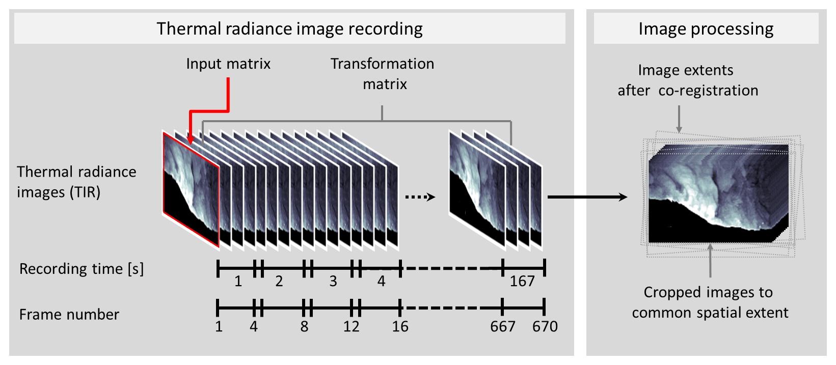
Figure 2Graphic illustration of image recording and image preprocessing applied during the presented approach.
To overcome the varying footprint, we define the first image of the set as the reference image and all remaining ones as input images (Fig. 2). Subsequently all input images are automatically co-registered onto the reference image using an intensity-based image registration within a MATLAB 2016 environment1. The applied image registration uses a similarity transformation that considers translation, rotation and scaling as possible factors induced by the UAV position variability and thus the non-congruent image footprints. This type of registration was chosen due to the fact that the short-term differences between images would not cause (i) nonlinear geometric differences or (ii) a change of intensities, which in the present case are radiances. Instead, the land and placed reflectors especially represent those rigid parts with similar intensities needed for intensity-based image registration (Kim and Fessler, 2004).
The core of the intensity-based image registration consists of comparing an input matrix (reference image) with a transformation matrix (each input image). During an iterative regular step gradient descent optimization, the transformation matrix is transformed, incorporating scaling, rotation and translation. The intensities of both the input and transformation matrices are compared using a similarity measure (e.g. a mean square metric as in the presented study) with the aim to maximize the similarity between both matrices (Viana et al., 2015). The iterative optimization process continues until the maximum iteration criterion reaches 1000 iterations, or the optimization criterion reaches a maximum step length of 0.01. This image registration process is repeated for all input images.
To provide a further independent accuracy measure, we use the two previously described aluminium reflectors. Similar to the automatic approach described in Holman et al. (2017) to find GPS targets, we define search windows in the registered input images, looking for the lowest radiance values (= reflector plates). Since the plates represent an area of several connected pixels, we then extract the mass centre of both plates and each image. Comparing the positions of the mass centres of both reflectors in the reference image with each input image yields an independent spatial accuracy measure. The so-obtained spatial accuracy of the image registration results in an RMSE of 0.58 pixels (1 pixel = 13 cm), a mean of 0.5 pixels, and a standard deviation of 0.3 pixels (see Fig. S1 in the Supplement).
As a consequence of the image registration process and the transformation of the input matrices, the footprint (covered area) varies. In order to be able to analyse the same covered area, we reduce the image sizes to a common footprint extent represented by all images. The so-obtained image size amounts to 561 pixels × 376 pixels. Onto all co-registered images, we then apply a manually derived land mask, masking out any radiances from land parts. Subsequently, radiance values of the remaining water area are normalized using a z-score normalization to account for potential global solar radiation differences that may occur over the time of investigation and would affect the result. The so-obtained processed image set consists of a 3-D data cube () of 670 images (hereafter frames) resembling a total time period of 167 s and showing normalized sea surface radiances in x,y dimensions.
3.2 Delineation of diffuse and focused SGD spots
Since SGD at the investigated site consists of focused SGD occurring offshore and diffuse SGD occurring at the land–water interface, we use different approaches to extract relevant discharge spots separately to finally pursue the intended temporal investigations. Given the assumption of a thermally stabilized area over time induced by focused SGD (Mallast et al., 2013b; Siebert et al., 2014), we calculate the thermal variance per pixel of the data cube's temporal dimension t using MATLAB 2016. The resulting low-variance areas represent focused SGD sites with constant and intense discharge. To extract focused SGD sites, we apply a subjective variance threshold of <0.0192 and eliminate extraction artefacts, using a morphological closing and deletion of objects smaller than 150 pixels to obtain the low-variance area representing focused SGD sites only.
In contrast, the observed diffuse SGD site along the shoreline discharges less water with lower discharge rates and thus has a smaller momentum, which inevitably leads to a smaller, thermally stabilized alongshore area (∼ 101−102 cm perpendicular to the coastline). While thermally stabilized, several direct forces such as breaking waves and currents influence the same area and thus the resulting thermal radiation pattern on the sea surface. These factors lead to rather high variances compared to focused SGD flow. Unfortunately, a similar variance can be expected from ambient areas influenced by highly dynamic flow field induced by waves, currents and discharge. As a consequence, we delineate diffuse SGD from a single frame (frame 210 – not shown) in which thermal radiation patterns and maximum spatial extents induced by high discharge rates are unequivocally detectable (a comparable single image is shown in Fig. 3, upper left image). Analogous to the focused SGD sites, we apply a subjective threshold of >2.5 (normalized radiation) to extract discharge-induced thermal patterns and eliminate extraction artefacts using a morphological closing to clean extracted pattern objects, followed by the deletion of objects smaller than 150 pixels to focus on larger patterns only.
3.3 Spatio-temporal analyses
We conduct two forms of (spatio-)temporal analyses: (i) a spatio-temporal analysis to identify the spatial variability of both thermal radiance patterns induced by diffuse and focused SGD and (ii) a periodicity analysis to reveal possible reoccurring temporal discharge patterns. To explore the spatio-temporal behaviour, and within a MATLAB 2016 environment, we construct transects across the maximum extent of each extracted SGD spot, as we expect the most pristine patterns there. Along each transect, normalized thermal radiances per frame are extracted, filtered using a 1-D ninth-order median filter to reduce the white noise portion, and finally plotted, highlighting the spatio-temporal behaviour for each spot.
For the periodicity analysis we use an autocorrelation function, which measures the self-similarity of a signal (Tzanetakis and Cook, 2002). If discharge occurs regularly, it causes a periodic signal, which is expressed as a significant peak (above or below 95 % confidence interval) in the autocorrelation function. As we expect the most pristine discharge-induced thermal pattern signals for both SGD types at the midpoint of each transect, we pursue the periodicity analysis at the specific transect midpoint pixel for each of the transects.
3.4 Water chemistry and inverse geochemical modelling
To draw conclusions about the karst maturity of the flow net that feeds on- and offshore springs, we investigate the type and intensity of groundwater–rock interaction at each spring based on their on-site and chemical parameters. Physicochemical on-site parameters (temperature, density, pH, electrical conductivity) of all the above mentioned focused SGD as well as onshore springs (see Fig. 1d, e) are measured in the field using a WTW 350i and Mettler Toledo density meter. The sampling procedure for groundwater samples to analyse the major element concentrations follows the procedure described in detail in Ionescu et al. (2012). Generally, samples for anion and cation analyses are filtered (0.22 µm CA filters), separately filled in HDPE bottles and stored under cool conditions. Cation samples are immediately acidified and later analysed by applying ICP-AES. Anions are analysed using ion chromatography and bicarbonate by Gran titration (see Table 2).
The individual water–rock interactions, which lead to the chemical composition of the respective groundwaters in the springs, are inversely modelled applying PHREEQC and Pitzer thermodynamic database. We apply the latter due to the high activities in the modelled environment, consisting of a sedimentary saline aquifer body, soaked with interstitial brine, which admixes to the fresh groundwater. On the basis of the abundant easily soluble minerals (halite, aragonite and gypsum), we select reactive solid phases in the sedimentary succession, enable ion exchange on clay minerals, and evaluated modelling results based on the probability and lowest sum of residuals.
It is a proven fact that SGD influences the sea surface temperature and thus the thermal radiances, and that it is thoroughly detectable given a sufficient temperature contrast between groundwater and sea or lake water and a certain minimum discharge volume and momentum (Johnson et al., 2008; Lee et al., 2016; Tamborski et al., 2015). Our results confirm this fact as diffuse SGD induces thermal radiance patterns with values >1 (higher temperatures) that are visible in Fig. 3a and spatially coincide with our field observations. Yet, the single thermal radiance image suggests the diffuse discharge occurs in two distinguishable patterns.
The first pattern is a coastal fringe of 35 m length and of 10 pixels (1.3 m) width, showing elevated normalized thermal radiance (NTR) values >1. This alongshore distribution exceeds the visual results of ca. 20 m by a factor of 1.5 and suggests a homogeneously distributed, low velocity and low rate discharge of warmer groundwater that emerges partially onshore and partially directly at the water–land interface (Fig. 3a).
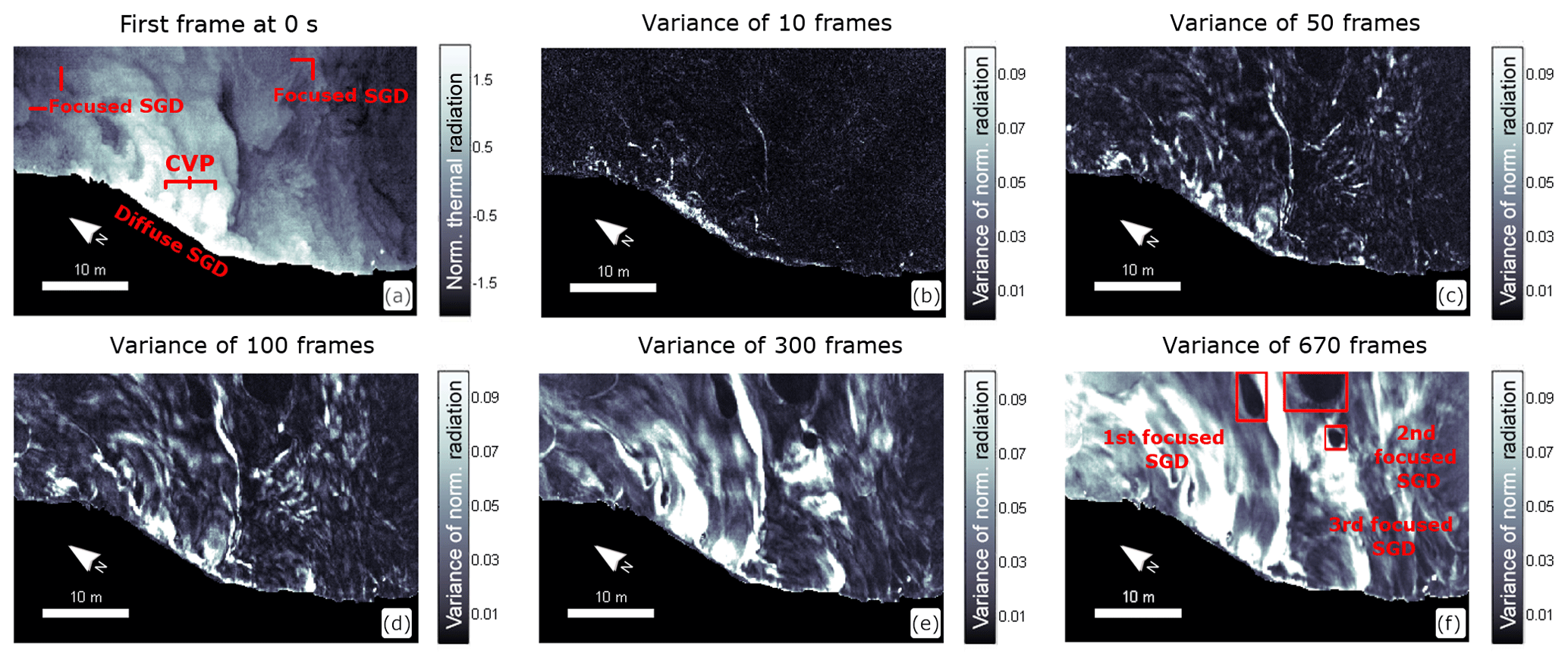
Figure 3Variance of normalized thermal radiances over time starting with a normalized thermal radiance image (a) showing ambiguous evidence of focused SGD spots, but distinct evidence of diffuse SGD and counter rotating vortex pairs (CVPs). The latter serves as an indication of a focused flow within the diffuse SGD area (a). The following panels show the integration of 10 (∼ 2.5 s), 50 (∼ 12.5 s), 100 (∼ 25 s), 300 (∼ 75 s), and 670 frames (∼ 167.5 s) as variance per pixel. The final image (f) shows three delineated focused SGD spots (red boxes) indicated through variance values <0.019.
The second, seemingly dominant pattern is characterized by NTR values >1, but in contrast to the first, it consists of distinctive counter-rotating vortex pair (CVP) flow structures (Cortelezzi and Karagozian, 2001), discernible based on the mushroom shape, with length axes between 20 and 46 pixels (2.6–6.0 m). The cause appears to be a focused and lateral jet-like discharge at four locations (Fig. 3a). Plumes, caused by both discharge forms, are subsequently deviated towards NNE.
Focused SGD with an expected circular to elliptical shape as observed by Mallast et al. (2014) and Swarzenski et al. (2001), are not unequivocally visible from the single frame (one thermal radiance image) only. At the upper and left ends of the single frame (first frame in Fig. 3), three half-circular patterns with NTR values between −0.6 and 0 foreshadow focused SGD spots, which coincide with in situ observed and sampled focused SGD spots 11∕120, 11∕121 and 12∕382. However, from the thermal radiation perspective, spatial indications for more than these three SGD sites are missing.
Given the assumption of SGD to thermally stabilize thermal radiance variation at the sea surface over time, as shown for satellite images (Schubert et al., 2014; Oehler et al., 2017), we integrate several frames (thermal radiance images) to enhance the above-mentioned focused SGD spots and to reveal further ones.
The thermal radiation variance of 10, 50 and 100 frames (integration of 2.5, 12.5 and 25 s respectively) already indicates thermally stable (variance values <0.2) and thermally labile areas (variance values ≥0.2). However, with larger integration times of 300 and 670 frames (integration of 75 and 176 s respectively), the three above-mentioned focused SGD spots appear, as well as two additional SGD spots in the upper part of the resulting variance image (Fig. 3f), which spatially coincide with in situ observed focused SGD sites 11∕101, and 11∕102. In the following sections, we focus on the three largely complete focused SGD spots 1 to 3 (Fig. 3). These three focused SGD spots exhibit variance values <0.019 and elliptical (first spot) to circular (second and third spot) shapes at the sea surface underlined by the individual length ∕ width ratios (Fig. 4). The lowest variance values, and therefore the thermally most stable areas are located at the southern end of the first and second SGD spots and on the northern end of the third SGD spot. Thermally indicated surface areas vary between 4.1 and 28.7 m2 despite similar spring depths of 13–20 m.
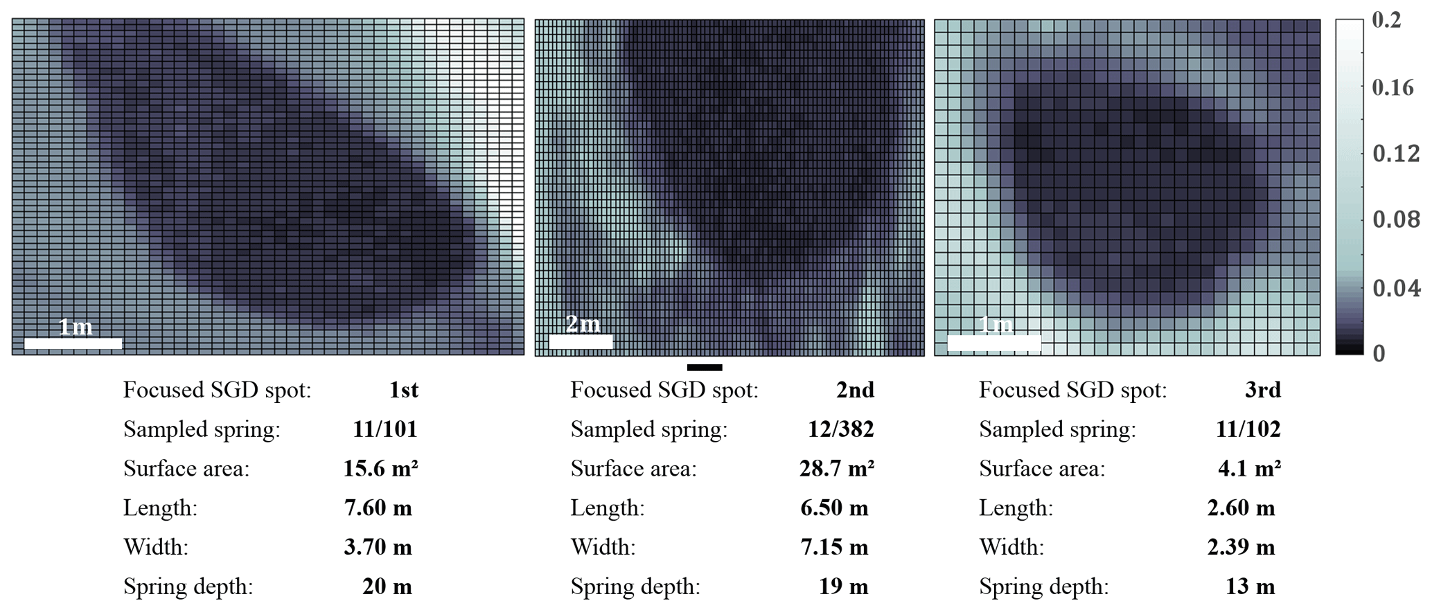
Figure 4Spatial characteristics of the presented focused SGD spots and their spatial correspondence of sampled submarine springs during previous campaigns.
4.1 Spatio-temporal behaviour of discharge-induced thermal radiance patterns
While the previous variance analysis highlights thermally stable and labile areas useful for identifying SGD spots, time- specific information on spatio-temporal discharge behaviour cannot be derived. We obtain this information through the introduction of transects (see left column in Figs. 5 and 6) along which we extract radiation values of each frame. The transects are constructed across the maximum spatial extent of each extracted, focused and diffuse SGD spot, as we expect the most pristine temporal patterns representative for each spot to occur here.
Table 1Summary of values characterizing the spatio-temporal behaviour of each focused and diffuse SGD spot.
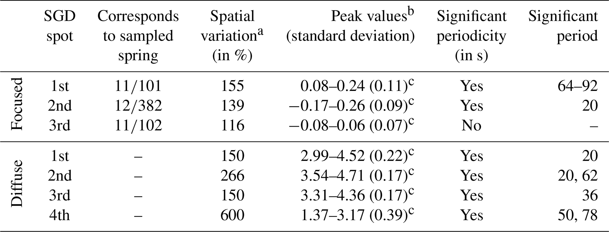
a For 90 % of the data. b Mean of the maximum values per frame over time c P value of <0.001 according to a Wilcoxon rank sum test, testing the significance of the peak values against non-peak values.
4.1.1 Spatio-temporal behaviour of focused SGD spots
The middle column of Fig. 5 shows the time series of NTR values along each SGD transect. Furthermore, SGD spot boundaries are indicated (white lines = maximum gradients of each transect profile), which provide an orientation for the spatio-temporal behaviour of each spot. The focus is set on the area in between the boundaries representing the area in which SGD governs the thermal radiation distribution. In the case of the first focused SGD spot that corresponds to sampled spring 11∕101, the location is rather stable with its centre between transect pixel 18 and 23 (spatial shift of <0.65 m). In contrast, its boundaries are highly dynamic resulting in a varying distance between 20 and 31 pixels (2.6 to 4.0 m respectively; for 90 % of the data) and thus a change of 155 % (Table 1). This dynamic partially follows a certain trend during which both boundaries (white lines) show a synchronous directional change over a certain period (e.g. frame 150–400). Within the SGD spot, NTR values peak around the transect centre and decrease towards both boundaries. This peak is higher during the first 300 frames, with NTR values of 0.24, and decreases slightly between frames 300 to 500 to values of 0.08 before it increases to values around 0.18 for the remaining frames.
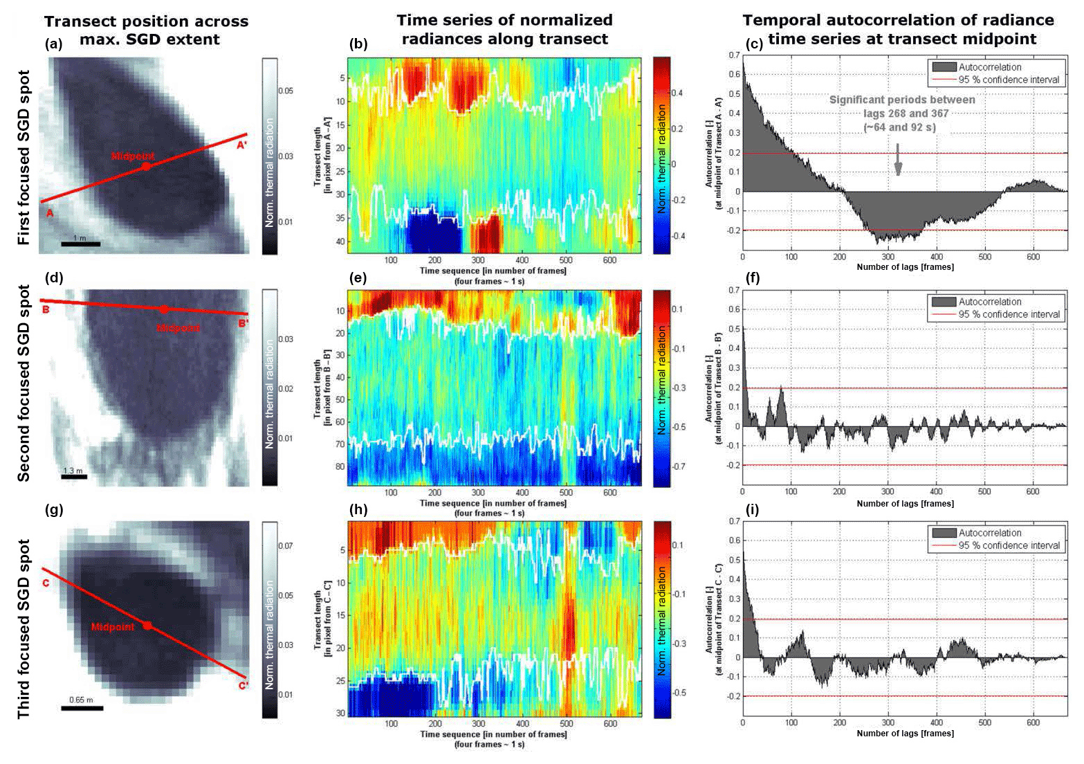
Figure 5Analyses of spatio-temporal behaviour and potential periodicity of SGD spots are presented. Panels (a), (d), (g) show transects across the maximum extent and midpoint position of the SGD spot (subsets correspond to the red boxes shown in Fig. 3; note that the spatial scale varies between each spot indicated through the scale bar at the lower left of each subset). Panels (b), (e), (h) show the normalized thermal radiance (NTR) values along transects over time. The white lines indicate the boundary of the focused SGD spots. Panels (c), (f), (i) show the temporal autocorrelation of the NTR values along the entire time series obtained at the midpoint of the transect as described in Sect. 2 to detect possible periodicities.
The centre of the second focused SGD spot, which corresponds to sampled spring 12∕382, shifts between transect pixels 40 and 45 (<0.65 m), indicating similar stable conditions. The boundary behaviour differs slightly from the first focused SGD spot. The lower boundary is rather stable, fluctuating around transect pixel 70, whereas the upper boundary describes on average a wave-like change between frames 1 and 300 before displaying a stable fluctuation around transect pixel 20. The resulting diameter of the second focused SGD spot is therefore between 43 and 60 pixels (5.59 to 7.8 m; for 90 % of the data) and thus shows a change of 139 % (Table 1). Compared to the first focused SGD spot, the absolute peak values of the second focused SGD spot of −0.26 and their general trend over time are lower. They display a rather random behaviour over all frames, with the exception of frames 485 to 520, during which the peak values (around −0.17) are higher.
The location of the third focused SGD spot, which corresponds to sampled spring 11∕102, centres between transect pixels 15 to 20. The spot's boundaries are stable during the first 200 frames, where they display a synchronous directional change similar to the first focused SGD spot. For the remaining frames, the lower boundary is highly dynamic and totally random while the upper is rather stable with less fluctuation until frame 350. The resulting boundary distance within the first 200 frames is between 18 and 21 pixels (2.34 and 2.73 m respectively; for 90 % of the data) and thus resembles a change of 116 % (Table 1). The peak values of −0.08 to 0.06 resemble those of the first and to a lesser extent those of the second focused SGD spot. Over time, they exhibit a similar random behaviour over all frames, with the exception of frames 485 to 520, during which the peak values are higher at 0.06.
4.1.2 Spatio-temporal behaviour of diffuse SGD spots
Analogous to the focused SGD spots, the middle column of Fig. 6 shows time series of the NTR values along the transects of each diffuse SGD spot to illuminate the spatio-temporal discharge behaviour. Apparent for the first, second, and third diffuse SGD spots are higher NTR values >4 for a constant transect length of 5–8 pixels (0.65–1.02 m) starting at the shoreline. Only the fourth diffuse SGD spot exhibits no constantly elevated NTR values over the entire observation time close to the shoreline. All spots show outburst-like events during which NTR values >3 occur. Among all spots, the onsets and influence lengths of these outburst events vary. While for the first spot the average influence length reaches 20 pixels (=2.60 m) for NTR values >3, the average length of the second is 33 pixels (=4.29 m). The third has a length of 20 pixels (2.60 m) and the fourth only 7 pixels (0.91 m). Consequently, the percentage change of the influence length axis is between 150 % for the first and third diffuse SGD spot, but amounts to 266 % for the second spot, and reaches up to 600 % for the fourth spot.
4.2 Periodicity analysis
The previous spatio-temporal behaviour already pointed at a certain recurrence pattern of the observed thermal radiation but lacked a distinct statement on whether or not it contains a significant periodicity and thus a dominating force inducing it. In order to provide an unequivocally and temporally pristine discharge signal, we analyse its temporal pattern based on a single pixel of each transect (midpoint of the transect) using a temporal autocorrelation analysis (right columns in Figs. 5 and 6 respectively).
4.2.1 Periodicity of focused SGD spots
Temporal autocorrelation of the first focused SGD spot distinctively differs from the second and third focused SGD spots. The first spot shows a small but significant negative autocorrelation of −0.25 between lags (frames) 268 and 367 (64–92 s), indicating a recurring pattern and hence a certain periodicity (Fig. 5). This observation matches the aforementioned peak value shift from 0.24 to 0.08 in the same frame region. The second focused SGD spot shows a small positive autocorrelation of 0.21 at lag (frame) 80, while remaining peaks vary in both directions, but below the confidence intervals. Both facts are distinctively different from the autocorrelation of the first focused SGD spot, but resemble the autocorrelation function of the third SGD spot, whose peaks are exclusively insignificant and reflect no periodicity indication.
4.2.2 Periodicity of diffuse SGD spots
Time series plots (middle column in Fig. 6) indicate a regular recurrence of thermal radiation values. This behaviour is underlined by the temporal autocorrelation of all diffuse SGD spots, which show a significant temporal autocorrelation that occurs at different lags and with mostly different intensities. While the first diffuse SGD spot exhibits only one significant period at lag 81 (20 s), the second spot shows two, one at lag 81 and a second one at lag 247 (62 s). Despite the spatial proximity of ca. 5 m to the first two diffuse SGD spots, the third diffuse SGD spot shows a different temporal autocorrelation, with one significant peak at lag 143 (36 s). Also different is the fourth spot, which exhibits two peaks at lag 198 (50 s) and lag 314 (78 s). All plots in the right column contain a reference autocorrelation function of a pixel close to the source point at the shoreline (transect pixel three). This reference shows high-frequency behaviour unlike the temporal, diffuse SGD, induced thermal radiation behaviour described before (except for the last diffuse SGD spot).
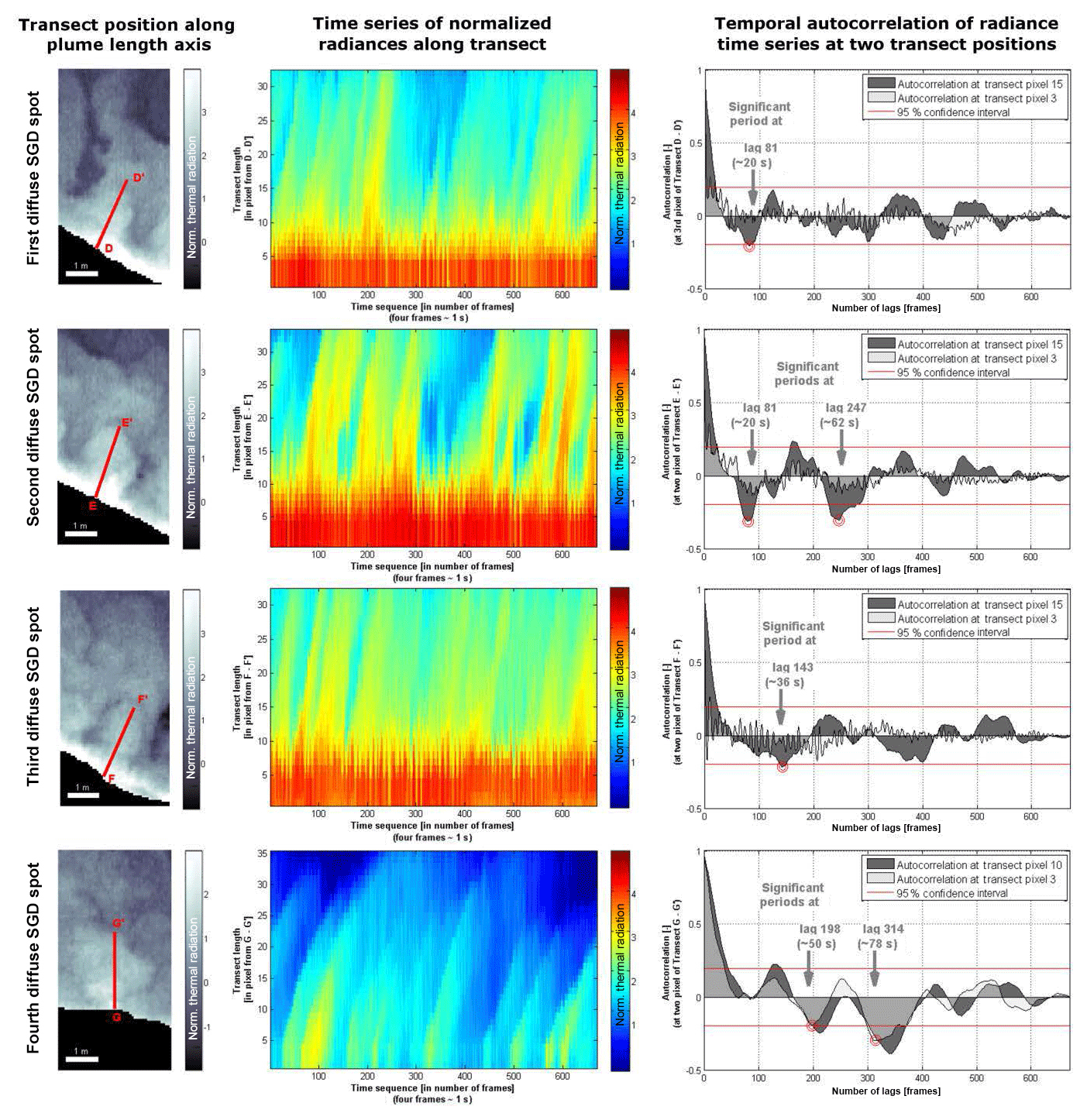
Figure 6Analyses of spatio-temporal behaviour and potential periodicity of diffuse SGD spots are presented. Spot locations are outlined in Figs. 1 and 3, indicated by the location of the counter rotating vortex pairs (CVPs). The first column shows transects across the maximum extent and midpoint position of diffuse SGD spots (note that the spatial scale varies between each spot indicated through the scale bar at the lower left of each subset). The middle column shows the normalized thermal radiance (NTR) values along transects over time. The third column shows the temporal autocorrelation of NTR values along the entire time series obtained at the midpoint of the transect. Those points reflect the most unaltered discharge signals (the larger value). As reference, we show the third transect pixel (close to the shoreline) as well in order to outline the wave influence on the periodicity.
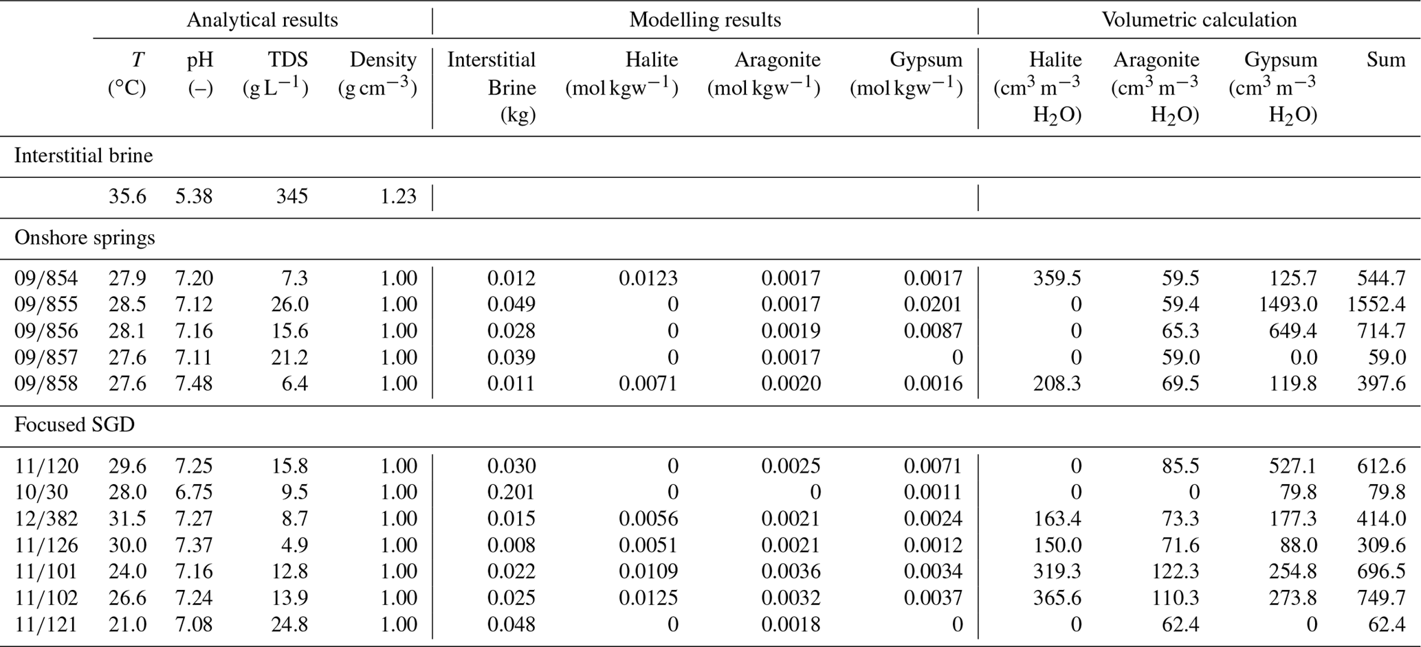
Table 2Water chemistry of all sampled focused SGD and onshore springs (some springs are located next to the study area and not shown in Fig. 1), along with the results from the inverse geochemical modelling and the volumetric calculation. Note that the volumetric calculation is based on the molar volume of halite (29.24 cm3 mol−1), aragonite (34.17 cm3 mol−1) and gypsum (74.29 cm3 mol−1). Also note that the information given here represents a summary of the most important information. Full details are given in Table S2 in the Supplement.
4.3 Water chemistry and inverse geochemical modelling
The samples focused on SGD and onshore springs discharge with a temperature between 21 to 31.5 ∘C. Though the groundwater of both focused SGD and onshore springs originates from the freshwater JGA, the springs discharge brackish water with salinities (TDS) ranging between 4.87 and 26.0 g L−1 with the tendency to be on average less saline onshore (TDS = 12.8 g L−1) compared to the focused SGD (TDS = 20.1 g L−1). The inverse geochemical modelling results indicate halite, aragonite and gypsum to be the most important minerals in solution, though ion exchange on clay minerals plays a significant role. Although discharge locations are very close, the amounts of dissolved halite (0–0.01 mol kg−1 H2O), aragonite (0–0.004 mol kg−1 H2O) and gypsum (0–0.02 mol kg−1 H2O) vary significantly between the different springs (Table 2). Translated into cavitation rates, emerging groundwater dissolves and relocates about 59.0–1.552.4 cm3 of halite, aragonite and gypsum per cubic metre from the passed branches of the groundwater flow net into the Dead Sea. Following the above-mentioned approach, those springs with the lowest water–rock interactions, which consequently emerge from the most mature karst pipes, are springs 09∕857, 10∕30, and 11∕121, which all have values <79.8 cm3 of halite, aragonite and gypsum per cubic metre of water. In contrast, springs 09∕855, 09∕856 or 11∕102 possess values >714.7 cm3 of halite, aragonite and gypsum per cubic metre water, which proves a higher water–rock interaction and thus intense dissolution activity that can only occur in less mature karst pipes (Table 2). Focused SGD spots reflect values of 696.5 and 749.7 cm3 (first and third spot respectively) and thus a less mature karst system, while the second focused SGD spot has the lowest value of 414.0 cm3 of halite, aragonite and gypsum per cubic metre of water and thus emerges from a more mature karst system.
The high spatial and temporal resolutions of the thermal radiation data show a highly dynamic setting with various discharge locations, patterns, and forces. Analysing the spatio-temporal behaviour of each SGD spot independent of its type reveals striking details: (i) it enhances focused SGD patterns otherwise being camouflaged by strong lateral flow dynamics and sheds light on crossflow influences, (ii) the spatio-temporal behaviour shows a thermal SGD pattern size variation over time of up to 155 % for focused SGDs and 600 % for diffuse SGDs due to different flow dynamics, and (iii) it reveals a periodicity for diffuse SGD. We discuss these aspects in the following sections and outline possible driving forces or causes, and we conclude with potentials for and limitations of the presented approach, including possible transferability to other locations.
5.1 Enhancing focused SGD
Deriving unequivocal SGD indications from single frames such as in Fig. 3 is not trivial, especially in a highly dynamic system as the one presented. For the present case, we suggest the following causes to be relevant:
- i.
lateral flow dynamics induced by diffuse discharge with higher temperatures (see point ii) govern the investigated area and superimpose thermal radiance signals from vertical flow of focused SGD as mentioned in Mallast et al. (2013a);
- ii.
entrainment of ambient water during the turbulent ascent (buoyant jet) of groundwater to the sea surface (Jirka, 2004) leads to a consequential adaption of temperature and thus the emitted thermal radiance; and
- iii.
potential groundwater discharge fluctuation with possibly very small to stagnant discharge rates, as described in Ionescu et al. (2012) for the presented site at the moment of recording, which lead to no traceable thermal radiance signal from SGD at the sea surface.
However, the above-mentioned possible relevant causes are all dynamic in spatial and temporal terms. Thus, accounting for the fact of a thermal stabilization at the sea surface as a consequence of a continuous discharge of equally tempered groundwater (Siebert et al., 2014) reveals thermally stable areas induced by SGD that might otherwise be undetectable. The thermal stabilization is accompanied by the interplay of fluid movements (lateral vs. vertical flow kinetics) and thus results in developing water surface geometries (wave structures), e.g. at the interface of opposing water flows. Surface geometries have an effect on the recorded thermal radiances due to the directional dependence of the surface emissivity (Norman and Becker, 1995; Cheng and Liang, 2014). Wave fronts, for example, with surfaces being orthogonal to the sensor (0∘), would have the highest thermal radiance values. As the angle to the sensor increases, recorded thermal radiances decrease, although the sea surface temperature is the same (Cheng and Liang, 2014). Thus, the temporal effects through thermal stabilization and changing surface geometries as a consequence of flow dynamics are the two governing drivers, which allow easy detection of focused SGD through the integration of thermal radiation over longer time periods. According to our findings, the thermal radiance variance over a period of 25 s (100 frames) already provides a sufficient basis to outline SGD areas (Fig. 2). Integrating over longer time periods emphasizes SGD areas, which consequently confirms the thermal radiance stabilization over time at the sea surface of a SGD-affected area (Siebert et al., 2014).
Apart from enhancing focused SGD occurrences, the shape of the focused SGD variance pattern at the sea surface along with the location of the lowest variance values (area most thermally stable) gives an indication of SGD emergence locations and the deflection of the resulting vertical plume until it reaches the sea surface. None of the three are perfectly circular, which would indicate an uninfluenced positive buoyancy of discharging water and a SGD emergence directly beneath the centre of the variance pattern (Jirka, 2004). Instead, they are all more or less elliptical, with the lowest variance values at the southern ends (first and second focused SGD spot) and at the northern ends (third focused SGD spot). The remarkable elliptical shape of the first focussed SGD spot implies a crossflow from the south causing a northward deflection of the vertical SGD plume and an elliptic shape of the horizontal plume pattern at the sea surface (Akar and Jirka, 1995). Less pronounced elliptical shapes but with the same northward deflection trend exhibit the second and third focused SGD spot. The northward deflection is most likely induced by flow dynamics as a consequence of diffuse SGD. Since the location of the diffuse SGD spots, especially those with distinctively periodic events with higher discharge rates (Fig. 3), is directly SSW and shows the same northward horizontal plume orientation, we suggest this discharge is the driving force for the deflection.
5.2 Spatio-temporal behaviour of SGD patterns
The variance image provides an average representation of all SGD spots, which are especially useful for reliable size–discharge comparison purposes between SGD spots and likewise allow SGD spots to be outlined. However, as the previous section points out, all are subject to external forces such as currents, waves, and the influence of internal discharge dynamics on resulting pattern shape and size characteristics of the thermal radiance pattern over time.
For focused SGD, the observed thermal radiance pattern sizes (distance between boundaries) over time show a spatial variation between 116 % (=2.3 m for the first focused SGD spot) and 155 % (=4.0 m for the third focused SGD spot) as shown in Fig. 5. The variance is a result of occurring lateral flow dynamics constantly influencing the pattern on the sea surface. Yet, the influence is anisotropic in space and time as the lateral flow dynamics are dominated by waves coming from the east and the interaction of horizontal SGD plumes on the sea surface (e.g. second and third focused SGD) as described in Teamah and Khairat (2015), but moreover the strong lateral flow dynamics (crossflow) induced by the discharge impulses of diffuse SGD that in the following is deflected to the NE. The interplay and constant temporal changes lead to an asynchronous boundary movement for most of the observed SGD-induced thermal radiance patterns. Only during the first 200 frames and for the first and third focused SGD spot did the asynchronous behaviour change to synchronous behaviour. During this time only one force seems to dominate the dynamic, causing the synchronous behaviour.
The SGD-induced thermal radiation pattern size variation is different for the observed diffuse SGD spots. While three out of four spots constantly influence a longshore area of 5–8 pixels (0.65–1.04 m), outburst-like events change the cross-shore influence length between 150 % and 600 % and between 0.60 and 4.29 m (Fig. 6). The constant influence reflects a continuous diffuse discharge with lower discharge rates. The latter, however, shows a focused flow with intermittent higher discharge rates. Higher discharge rates induce a higher momentum and consequentially increase the influenced area off the discharge spot. In turn it reveals that karst conduits exist close to the shoreline and next to diffuse SGD. The intermittency with a seemingly recurring temporal pattern, however, points to a steady interplay of different forces that is the subject of the next section.
5.3 Periodicity of diffuse SGD
For focused SGD spots, we could not reveal a significant periodicity, either because of the limited observation length or because no periodicity exists. For diffuse SGD spots, the temporal autocorrelation analysis reveals significant periodicities. The periodicity of discharge rate events varies significantly among given spots between 20 and 78 s (right column in Fig. 6). It primarily provides a further example of the high temporal discharge variability over small spatial scales which, normally, is due to tides or wave set-up that change hydrostatic pressure conditions (Taniguchi et al., 2003b; Burnett et al., 2006). For the present case, tidal influences are irrelevant as the tidal cycles do not exist at the study site. Wave influence on the other hand cannot be excluded, per se. However, most likely it is not the main cause since observed wave frequency of 3 to 7 s would cause high-frequency discharge intermittency of the same magnitude. Precisely this high frequency is observable in the autocorrelation graphs of Fig. 6 close to the shoreline (transect pixel 3). Thus, the frequency proves the minor wave influence on the main discharge events with an observed frequency that is up to 10 magnitudes larger. Along with the focused discharge nature, it rather points to an interplay between wave set-up and a geometry effect within conduits of groundwater flow as the underlying mechanism as described for karst areas in Smart and Ford (1986). Discharge behaviour in this case depends on the maturity and geometric formation of the conduit network. Following Surić et al. (2015) the discharge behaviour is highly anisotropic and heterogeneous, and features a rapid flow. The anisotropic and heterogeneous discharge behaviour is furthermore underlined by the discharge onset and the periodicity that is unequal among the individual spots, even though their spatial location is within 10 m distance (Fig. 3).
According to the modelling results, groundwater passes the DSG through several subaquifers as described in Yechieli et al. (2010), and most probably via conduits, which develop through the fuzzy dissolution of easily soluble minerals that make up large percentages of the sedimentary body. It is further assumed, due to the impregnation of the sediment by Dead Sea brine, that cavitation activity is lower closer and below the freshwater–saltwater interface, although it exists and leads to abundant submarine springs. However, groundwater may also reach the Dead Sea through open faults, which may deeply fracture the sedimentary body as a result of active rift tectonics. Further preferential groundwater pathways may also be created through shallow cracks that develop through the relaxation of the sediment due to the gravitational release of interstitial brine.
However, for whatever reason fresh groundwater is allowed to invade the DSG due to the omnipresent abundance of easily soluble minerals, dissolution activities will immediately start and will enlarge hydraulic apertures of the initial pathways through the sedimentary body. Cavitation rates may be dependent on boundary conditions (e.g. supply of freshwater, hydraulic gradient and microbial activity), leading to different degrees of conduit maturity and random conduit–network geometry.
Consequently, it is thoroughly possible that an initial anisotropic flow system is about to develop close to the observed shoreline. In interaction with the wave set-up, we suggest that such a randomly developed initial flow system is the cause for the different onsets and influence areas for the observed outburst-like events.
5.4 Potentials, limitations and potential errors
The hovering of the UAV over a predefined location and the sensing of thermal radiation at a rate of 4–5 Hz allows a combination of the continuous temporal with the continuous spatial scale for SGD research. In this context it bears an enormous potential as it is possible to provide detailed and high-resolution information on SGD dynamics but also on external forces influencing it. The potential includes the high temporal resolution (sampling intervals), which differs by 1 order of magnitude from classical in situ measurement intervals of 101–102 min (Cable et al., 1997; Mulligan and Charette, 2006; Michael et al., 2011), allowing the illumination of short-term discharge dynamics that could not be reflected with classical methods. The potential furthermore concerns the spatio-temporal continuous characteristic of the presented approach. With the unequivocal indication regarding where diffuse or focused SGD occurs, and where exactly the transition between SGD and ambient fluids is, the indication is that proper sampling sites for each of them could not have been done with a subjective selection of sampling sites. Thus, applying the presented approach before pursuing in situ sampling (which includes the selection of proper sampling sites and sampling intervals) is undoubtedly advantageous.
The third potential concerns SGD monitoring and especially SGD quantification purposes. As mentioned in the Introduction, the basis for SGD quantification is the size of thermal radiance patterns (plumes) in most studies (Kelly et al., 2018; Mallast et al., 2013a; Tamborski et al., 2015; Lee et al., 2016). The presented results show a spatial variation of 150 %–600 %, which indicates the possible uncertainty that underlies a quantification based on single thermal infrared images. With the presented approach these uncertainties could be specified, which, in turn, increases the explanatory power of the quantification.
Apart from these potentials, the approach bears limitations and potential errors that need to be accounted for, if the presented approach is to be applicable to different locations. The first limitation concerns the need for rigid image parts, such as land, to be able to pursue a proper image registration. Equal share of land and water parts, as in the present case, increases the accuracy and thus reduces the potential error due to an erroneous intensity-based image registration, but reduces the investigable area spatially and limits it to areas close to the shoreline. The shoreline bond could be overcome by using rigidly fixed buoys and mounted aluminium plates on top as ground control points anchored offshore. While the investigable area is maximized, the image registration needs to be changed to a procedure based on control points to determine the image transformation and thus the registration as described, for example, in Holman et al. (2017), since the intensity of an image cannot be taken as the basis.
However, independent of the selected approach and the land–water share, flight altitude and camera lens define the size of the footprint and thus the spatial coverage. Due to regulatory framework, flight altitudes are usually restricted, which consequently limits the maximum possible footprint. Thus the restricted flight altitudes represent another spatial limitation of the approach.
The aforementioned spatial limitations are furthermore accompanied by temporal limitations and errors. These temporal limitations are given by the flight times of present-day UAVs that reach up to tens of minutes (Floreano and Wood, 2015). Continuous investigations for several hours, days, or beyond have been, to date, impossible. This sort of long-term and continuous investigation for monitoring purposes, for example, could be possible using a thermal camera system fixed to a mast making flight times irrelevant. Despite other factors coming into play with fixed cameras, such as the viewing angle dependency on emissivity (Norman and Becker, 1995) and the addition of a changing solar reflection component to thermal emission during the day vs. solely thermal emission during the night, the potential lies in the generation of a thermal radiation time series and trend analyses, for example. Similar approaches using fixed video and camera systems, operating in the visible spectrum (red–green–blue, RGB), are operational for near-shore monitoring and management purposes (Holman et al., 2003; Taborda and Silva, 2012). Adapting these operational approaches to fixed thermal camera systems would mean overcoming temporal limitations on the presented UAV approach and generating unforeseen potential in SGD research.
Further limitations concern sensors. A geometric error can be introduced by lens characteristics which distort the thermal image. In particular, a wide-angle lens produces geometric distortions (Meier et al., 2011; Vidas et al., 2012) that can be corrected in order to achieve an image projection that matches the true projection surface. A further sensor limitation is a possible radiometric error. All uncooled microbolometers, including the one applied, have the disadvantage that a thermal drift could occur (Mesas-Carrascosa et al., 2018). Caused by effects of the ambient temperature on the microbolometer detector housing and the consequential energy dissipation from the housing onto the detector array, the thermal drift leads to a non-uniform influence on the thermal image, which manifests in a vignetting effect with radiance reduction towards the borders of a recorded image relative to its projection centre (Meier et al., 2011). Since it additionally changes with time (Wolf et al., 2016), this drift, especially for long term investigations, needs to be accounted for, otherwise Mesas-Carrascosa et al. (2018) estimate the temperature error to increase by 0.7 ∘C min−1.
The aforementioned limitations are all of a technical nature. However, we need to emphasize that natural limitations may also exist that may affect the result. The most prominent factor is the temperature difference between groundwater and ambient water. With a difference approaching 0 ∘C, an unequivocal differentiation is almost impossible, especially if we include entrainment of ambient water and thus the temperature adaption. The higher the difference, the more likely the possibility of identifying SGD-induced thermal anomalies in single images, but also of using a time series of thermal radiance images – as in the presented approach. The advantage of time series data is that the temporal dimension includes dynamics which may enhance subtle temperature differences. These dynamics may be due to waves in which the surface geometries provide the direct indication rather than the surface temperature (recall the directional dependence of the surface emissivity on recorded radiances – see Sect. 5.1). Hence, time series data, whether from an UAV platform or from a mast, are thoroughly recommendable.
Further limitations may exist due to parallel existing strong lateral flow dynamics, as in the present case. On single thermal radiation images, these dynamics may camouflage further focused SGD sites, especially at sites with low groundwater–ambient water temperature differences. Strong lateral dynamics may also, as in the present case, camouflage any bathymetry effect on thermal radiation images as it is described in Xie et al. (2002). If bathymetry has affected the sea surface temperature, we could detect a gradual decrease in temperature from the shoreline towards the sea centre. The reason that we cannot detect any gradual decrease, apart from the camouflaging lateral flow dynamics, may be the bathymetry itself. While the bathymetry decreases gradually during the first 30 m until about 10 m, SGD is found at the bottom of steep walls in depths of up to 30 m (Ionescu et al., 2012) in distances of 50 m to the coastline, which is also visible in Fig. 1a. This sudden morphological step may additionally cause the disappearance of the gradual temperature decrease usually triggered by bathymetry. However, we cannot exclude this effect occurring in other places and different settings where, for example, the bathymetry consists of uniform slopes . In these occasions, the bathymetry would cause higher sea surface temperatures in summer and lower sea surface temperatures in winter that may be accounted for in the case of SGD detection.
As pointed out, for most technical limitations, solutions and corrections exist to improve and adopt the presented approach independent of the study sites' characteristics. Thus, we propose that the approach is applicable to other areas with diffuse or focused SGD, since the general requirements consist of an UAV with a mounted thermal camera system and rigid areas or fixed points within the covered footprint to allow a proper co-registration of all thermal images. The applicability of the presented approach concerning natural limitations needs to be investigated in the future. However, given a certain discharge rate and sufficient temperature differences between groundwater and ambient water, the suggestion is that time series data of thermal radiance images could prove to be a promising tool for SGD investigations.
Hovering with an UAV over a predefined location recording thermal radiances at a temporal resolution of 4–5 Hz is a novel application technique combining continuous spatial and temporal scales. Based on the combination, we enhance focused SGD patterns that are otherwise camouflaged by strong lateral flow dynamics that may not be observed on single thermal radiation images. We furthermore show the spatio-temporal behaviour of a SGD-induced thermal radiation pattern to vary in size and over time by up to 155 % for focused SGDs and by up to 600 % for diffuse SGDs due to different underlying flow dynamics. We want to emphasize this aspect as it is important for SGD monitoring and especially SGD quantification purposes, which rely on single thermal radiation images and thus temporal snapshots that may not provide the entire picture. And lastly, we are able to reveal a short-term periodicity of the order of 20 to 78 s for diffuse SGD, which we attribute to an interplay between conduit maturity or geometry and wave set-up. The observed periodicity differs by 1 order of magnitude from classical in situ measurement intervals, which would not be able to detect the temporal behaviour we observe.
Since SGD, independent of its type, is highly heterogeneous in space and time, as we have also shown in our study, we suggest, where possible, inclusion of the presented approach before any in situ sampling to identify proper sampling locations and intervals. In this way, SGD investigations, especially in systems with complex flow, will be able to optimize their sampling strategies and possibly improve their results.
Raw thermal infrared radiation data are available online at: https://doi.org/10.1594/PANGAEA.898377.
The supplement related to this article is available online at: https://doi.org/10.5194/hess-23-1375-2019-supplement.
UM and CS conducted the experiment, UM analysed the data and drafted the paper. Both authors revised the paper and approved the final version.
The authors declare that they have no conflict of interest.
This article is part of the special issue “Environmental changes and hazards in the Dead Sea region (NHESS/ACP/HESS/SE inter-journal SI)”. It is not associated with a conference.
This work was financed by the DESERVE Virtual Institute, funded by the Helmholtz Association of German Research Centers (VH-VI-527) and a scholarship from the German Federal Ministry of Education and Research (YSEP97). Personal thanks are addressed to Yossi Yechieli and Gideon Baer (both Geological Survey of Israel) for the kind support, warm welcome, and unconditional assistance before and during the exchange of UM, including the logistical help. Meteorological data were provided by KIT (Jutta Metzger). This paper has benefited from the efforts, insightful comments and additions of two anonymous reviewers to whom we are eternally grateful.
The manuscript is dedicated to the memory of our deceased colleague and mentor Hans
Neumeister.
The article processing charges for this open-access
publication were covered by a Research
Centre of the Helmholtz Association.
Edited by: Efrat Morin
Reviewed by: two anonymous referees
Akar, P. J. and Jirka, G. H.: Buoyant spreading processes in pollutant transport and mixing Part 2, Upstream spreading in weak ambient current, J. Hydraul. Res., 33, 87–100, 1995.
Burg, A., Yechieli, Y., and Galili, U.: Response of a coastal hydrogeological system to a rapid decline in sea level; the case of Zuqim springs, The largest discharge area along the Dead Sea coast, J. Hydrol., 536, 222–235, https://doi.org/10.1016/j.jhydrol.2016.02.039, 2016.
Burnett, W. C., Aggarwal, P. K., Aureli, A., Bokuniewicz, H., Cable, J. E., Charette, M. A., Kontar, E., Krupa, S., Kulkarni, K. M., Loveless, A., Moore, W. S., Oberdorfer, J. A., Oliveira, J., Ozyurt, N., Povinec, P., Privitera, A. M. G., Rajar, R., Ramessur, R. T., Scholten, J., Stieglitz, T., Taniguchi, M., and Turner, J. V.: Quantifying submarine groundwater discharge in the coastal zone via multiple methods, Sci. Total Environ., 367, 498–543, https://doi.org/10.1016/j.scitotenv.2006.05.009, 2006.
Cable, J., Burnett, W., Chanton, J., Corbett, D., and Cable, P.: Field evaluation of seepage meters in the coastal marine environment, Estuarine, Coast. Shelf Sci., 45, 367–375, 1997.
Cheng, J. and Liang, S.: Effects of Thermal-Infrared Emissivity Directionality on Surface Broadband Emissivity and Longwave Net Radiation Estimation, IEEE Geosci. Remote S., 11, 499–503, https://doi.org/10.1109/LGRS.2013.2270293, 2014.
Cortelezzi, L. and Karagozian, A. R.: On the formation of the counter-rotating vortex pair in transverse jets, J. Fluid Mech., 446, 347–373, 2001.
Floreano, D. and Wood, R. J.: Science, technology and the future of small autonomous drones, Nature, 521, 460, https://doi.org/10.1038/nature14542, 2015.
FLIR® Systems: Tau® 2 Uncooled Cores, available at: http://www.flir.com/cores/display/?id=54717, last access: 16 December 2016.
Holman, R., Stanley, J., and Ozkan-Haller, T.: Applying video sensor networks to nearshore environment monitoring, IEEE Pervas. Comput., 2, 14–21, 2003.
Holman, R. A., Holland, K. T., Lalejini, D. M., and Spansel, S. D.: Surf zone characterization from Unmanned Aerial Vehicle imagery, Ocean Dynam., 61, 1927–1935, https://doi.org/10.1007/s10236-011-0447-y, 2011.
Holman, R. A., Brodie, K. L., and Spore, N. J.: Surf Zone Characterization Using a Small Quadcopter: Technical Issues and Procedures, IEEE T. Geosci. Remote, 55, 2017–2027, https://doi.org/10.1109/TGRS.2016.2635120, 2017.
Ionescu, D., Siebert, C., Polerecky, L., Munwes, Y. Y., Lott, C., Häusler, S., Bižić-Ionescu, M., Quast, C., Peplies, J., Glöckner, F. O., Ramette, A., Rödiger, T., Dittmar, T., Oren, A., Geyer, S., Stärk, H.-J., Sauter, M., Licha, T., Laronne, J. B., and de Beer, D.: Microbial and Chemical Characterization of Underwater Fresh Water Springs in the Dead Sea, Plos One, 7, e38319, https://doi.org/10.1371/journal.pone.0038319, 2012.
Jirka, G. H.: Integral model for turbulent buoyant jets in unbounded stratified flows, Part I: Single round jet, Environ. Fluid Mech., 4, 1–56, 2004.
Johnson, A. G., Glenn, C. R., Burnett, W. C., Peterson, R. N., and Lucey, P. G.: Aerial infrared imaging reveals large nutrient-rich groundwater inputs to the ocean, Geophys. Res. Lett., 35, 15601–15606, https://doi.org/10.1029/2008gl034574, 2008.
Kelly, J. L., Dulai, H., Glenn, C. R., and Lucey, P. G.: Integration of aerial infrared thermography and in situ radon-222 to investigate submarine groundwater discharge to Pearl Harbor, Hawaii, USA, Limnol. Oceanogr., 64, 238–257, doi:10.1002/lno.11033, 2018.
Kim, J. and Fessler, J. A.: Intensity-based image registration using robust correlation coefficients, IEEE T. Med. Imaging, 23, 1430–1444, 2004.
Lee, E., Yoon, H., Hyun, S. P., Burnett, W. C., Koh, D. C., Ha, K., Kim, D. J., Kim, Y., and Kang, K. M.: Unmanned aerial vehicles (UAVs)-based thermal infrared (TIR) mapping, a novel approach to assess groundwater discharge into the coastal zone, Limnol. Oceanogr.-Meth., 14, 725–735, https://doi.org/10.1002/lom3.10132, 2016.
Lewandowski, J., Meinikmann, K., Ruhtz, T., Pöschke, F., and Kirillin, G.: Localization of lacustrine groundwater discharge (LGD) by airborne measurement of thermal infrared radiation, Remote Sens. Environ., 138, 119–125, 2013.
Magal, E., Weisbrod, N., Yakirevich, A., Kurtzman, D., and Yechieli, Y.: Line-Source Multi-Tracer Test for Assessing High Groundwater Velocity, Ground Water, 48, 892–897, https://doi.org/10.1111/j.1745-6584.2010.00707.x, 2010.
Mallast, U., Schwonke, F., Gloaguen, R., Geyer, S., Sauter, M., and Siebert, C.: Airborne Thermal Data Identifies Groundwater Discharge at the North-Western Coast of the Dead Sea, Remote Sens., 5, 6361–6381, https://doi.org/10.3390/rs5126361, 2013a.
Mallast, U., Siebert, C., Wagner, B., Sauter, M., Gloaguen, R., Geyer, S., and Merz, R.: Localisation and temporal variability of groundwater discharge into the Dead Sea using thermal satellite data, Environ. Earth Sci., 69, 587–603, https://doi.org/10.1007/s12665-013-2371-6, 2013b.
Mallast, U., Gloaguen, R., Friesen, J., Rödiger, T., Geyer, S., Merz, R., and Siebert, C.: How to identify groundwater-caused thermal anomalies in lakes based on multi-temporal satellite data in semi-arid regions, Hydrol. Earth Syst. Sci., 18, 2773–2787, https://doi.org/10.5194/hess-18-2773-2014, 2014.
Meier, F., Scherer, D., Richters, J., and Christen, A.: Atmospheric correction of thermal-infrared imagery of the 3-D urban environment acquired in oblique viewing geometry, Atmos. Meas. Tech., 4, 909–922, https://doi.org/10.5194/amt-4-909-2011, 2011.
Mejías, M., Ballesteros, B. J., Antón-Pacheco, C., Domínguez, J. A., Garcia-Orellana, J., Garcia-Solsona, E., and Masqué, P.: Methodological study of submarine groundwater discharge from a karstic aquifer in the Western Mediterranean Sea, J. Hydrol., 464, 27–40, https://doi.org/10.1016/j.jhydrol.2012.06.020, 2012.
Mesas-Carrascosa, F.-J., Pérez-Porras, F., Meroño de Larriva, J., Mena Frau, C., Agüera-Vega, F., Carvajal-Ramírez, F., Martínez-Carricondo, P., and García-Ferrer, A.: Drift Correction of Lightweight Microbolometer Thermal Sensors On-Board Unmanned Aerial Vehicles, Remote Sens., 10, 615, https://doi.org/10.3390/rs10040615, 2018.
Michael, H. A., Lubetsky, J. S., and Harvey, C. F.: Characterizing submarine groundwater discharge: a seepage meter study in Waquoit Bay, Massachusetts, Geophys. Res. Lett., 30, https://doi.org/10.1029/2002GL016000, 2003.
Michael, H. A., Charette, M. A., and Harvey, C. F.: Patterns and variability of groundwater flow and radium activity at the coast: A case study from Waquoit Bay, Massachusetts, Mar. Chem., 127, 100–114, https://doi.org/10.1016/j.marchem.2011.08.001, 2011.
Mulligan, A. E. and Charette, M. A.: Intercomparison of submarine groundwater discharge estimates from a sandy unconfined aquifer, J. Hydrol., 327, 411–425, 2006.
Norman, J. M. and Becker, F.: Terminology in thermal infrared remote sensing of natural surfaces, Remote Sens. Rev., 12, 159–173, https://doi.org/10.1080/02757259509532284, 1995.
Oehler, T., Eiche, E., Putra, D., Adyasari, D., Hennig, H., Mallast, U., and Moosdorf, N.: Timing of land-ocean groundwater nutrient fluxes from a tropical karstic region (southern Java, Indonesia), Hydrol. Earth Syst. Sci. Discuss., https://doi.org/10.5194/hess-2017-621, 2017.
Schubert, M., Scholten, J., Schmidt, A., Comanducci, J. F., Pham, M. K., Mallast, U., and Knoeller, K.: Submarine Groundwater Discharge at a Single Spot Location: Evaluation of Different Detection Approaches, Water, 6, 584–601, 2014.
Siebert, C., Rödiger, T., Mallast, U., Gräbe, A., Guttman, J., Laronne, J. B., Storz-Peretz, Y., Greenman, A., Salameh, E., and Al-Raggad, M.: Challenges to estimate surface-and groundwater flow in arid regions: The Dead Sea catchment, Sci. Total Environ., 485, 828–841, 2014.
Smart, C. and Ford, D.: Structure and function of a conduit aquifer, Can. J. Earth Sci., 23, 919–929, 1986.
Surić, M., Lončarić, R., Buzjak, N., Schultz, S. T., Šangulin, J., Maldini, K., and Tomas, D.: Influence of submarine groundwater discharge on seawater properties in: Rovanjska-Modrič karst region (Croatia), Environ. Earth Sci., 74, 5625–5638, https://doi.org/10.1007/s12665-015-4577-2, 2015.
Swarzenski, P. W., Reich, C. D., Spechler, R. M., Kindinger, J. L., and Moore, W. S.: Using multiple geochemical tracers to characterize the hydrogeology of the submarine spring off Crescent Beach, Florida, Chem. Geol., 179, 187–202, https://doi.org/10.1016/S0009-2541(01)00322-9, 2001.
Taborda, R. and Silva, A.: COSMOS: A lightweight coastal video monitoring system, Comput. Geosci., 49, 248–255, 2012.
Tamborski, J. J., Rogers, A. D., Bokuniewicz, H. J., Cochran, J. K., and Young, C. R.: Identification and quantification of diffuse fresh submarine groundwater discharge via airborne thermal infrared remote sensing, Remote Sens. Environ., 171, 202–217, https://doi.org/10.1016/j.rse.2015.10.010, 2015.
Taniguchi, M., Burnett, W. C., Cable, J. E., and Turner, J. V.: Assessment methodologies for submarine groundwater discharge, in: Land and Marine Hydrogeology, edited by: Taniguchi, M., Wang, K., and Gamo, T., Elsevier, Amsterdam, 1–23, 2003a.
Taniguchi, M., Burnett, W. C., Smith, C. F., Paulsen, R. J., O'Rourke, D., Krupa, S. L., and Christoff, J. L.: Spatial and temporal distributions of submarine groundwater discharge rates obtained from various types of seepage meters at a site in the Northeastern Gulf of Mexico, Biogeochemistry, 66, 35–53, https://doi.org/10.1023/B:BIOG.0000006090.25949.8d, 2003b.
TeAx Technology: Thermal Capture, available at: http://thermalcapture.com/category/products/recordingsolutions/, last access: 16 December 2016.
Tzanetakis, G. and Cook, P.: Musical genre classification of audio signals, IEEE T. Speech Audi. P., 10, 293–302, 2002.
Viana, I., Orteu, J.-J., Cornille, N., and Bugarin, F.: Inspection of aeronautical mechanical parts with a pan-tilt-zoom camera: an approach guided by the computer-aided design model, J. Electron. Imaging, 24, 061118, https://doi.org/10.1117/1.JEI.24.6.061118, 2015.
Vidas, S., Lakemond, R., Denman, S., Fookes, C., Sridharan, S., and Wark, T.: A mask-based approach for the geometric calibration of thermal-infrared cameras, IEEE T. Instrum. Meas., 61, 1625–1635, 2012.
Vollmer, M.: Newton's law of cooling revisited, Eur. J. Phys., 30, 1063, https://doi.org/10.1088/0143-0807/30/5/014, 2009.
Wolf, A., Pezoa, J. E., and Figueroa, M.: Modeling and Compensating Temperature-Dependent Non-Uniformity Noise in IR Microbolometer Cameras, Sensors, Basel, Switzerland, 16, 1121, https://doi.org/10.3390/s16071121, 2016.
Xie, S.-P., Hafner, J., Tanimoto, Y., Liu, W. T., Tokinaga, H., and Xu, H.: Bathymetric effect on the winter sea surface temperature and climate of the Yellow and East China Seas, Geophys. Res. Lett., 29, 2228, https://doi.org/10.1029/2002GL015884, 2002.
Yechieli, Y., Ronen, D., Berkowitz, B., Dershowitz, W. S., and Hadad, A.: Aquifer Characteristics Derived From the Interaction Between Water Levels of a Terminal Lake (Dead Sea) and an Adjacent Aquifer, Water Resour. Res., 31, 893–902, https://doi.org/10.1029/94wr03154, 1995.
Yechieli, Y., Shalev, E., Wollman, S., Kiro, Y., and Kafri, U.: Response of the Mediterranean and Dead Sea coastal aquifers to sea level variations, Water Resour. Res., 46, W12550, https://doi.org/10.1029/2009wr008708, 2010.
The MATLAB code used for the present study can be distributed upon request.
Note that the subjective variance threshold is optimal for the present case and will certainly change in other environments. Thus, in order to investigate any spatio-temporal SGD analysis, this threshold needs to be adapted otherwise it would create an erroneous focused SGD outline and hence a wrong focus area.