the Creative Commons Attribution 4.0 License.
the Creative Commons Attribution 4.0 License.
 | 18 Mar 2019
Technical note: Laboratory modelling of urban flooding: strengths and challenges of distorted scale models
Sébastien Erpicum
Martin Bruwier
Emmanuel Mignot
Pascal Finaud-Guyot
Pierre Archambeau
Michel Pirotton
Benjamin Dewals
Laboratory experiments are a viable approach for improving process understanding and generating data for the validation of computational models. However, laboratory-scale models of urban flooding in street networks are often distorted, i.e. different scale factors are used in the horizontal and vertical directions. This may result in artefacts when transposing the laboratory observations to the prototype scale (e.g. alteration of secondary currents or of the relative importance of frictional resistance). The magnitude of such artefacts was not studied in the past for the specific case of urban flooding. Here, we present a preliminary assessment of these artefacts based on the reanalysis of two recent experimental datasets related to flooding of a group of buildings and of an entire urban district, respectively. The results reveal that, in the tested configurations, the influence of model distortion on the upscaled values of water depths and discharges are both of the order of 10 %. This research contributes to the advancement of our knowledge of small-scale physical processes involved in urban flooding, which are either explicitly modelled or parametrized in urban hydrology models.
- Article
(2461 KB) -
Supplement
(3142 KB) - BibTeX
- EndNote


Worldwide, floods are the most frequent natural disasters, and they cause over one-third of overall economic losses due to natural hazards (UNISDR, 2015). Flood losses are particularly severe in urban environments, and urban flood risk is expected to further increase over the 21st century (Chen et al., 2015; Hettiarachchi et al., 2018; Lehmann et al., 2015; Mallakpour and Villarini, 2015). In response, concepts such as water-sensitive urban design, low impact development and the sponge city model are rapidly developing (Gaines, 2016; Liu, 2016; Zhou et al., 2018). However, the design and sizing of measures aiming at enhancing urban flood protection require accurate tools for risk modelling and scenario analysis (Wright, 2014).
Specifically, reliable predictions of flood hazard are a prerequisite for supporting flood risk management policies. This includes the accurate estimation of inundation extent, spatial distribution of water depth, discharge partition and flow velocity in urbanized flood-prone areas, since these parameters are critical inputs for flood impact modelling (Dottori et al., 2016; Kreibich et al., 2014; Molinari and Scorzini, 2017). State-of-the-art numerical inundation models benefit from increasingly available remote sensing data, such as laser altimetry (e.g. Ichiba et al., 2018). Nonetheless, their validation for urban flood configurations remains incomplete because reference data from the field are relatively scarce and, to a great extent, inadequate (Dottori et al., 2013). Mostly watermarks and aerial imagery are available, but they remain uncertain and insufficient (e.g. inadequate time resolution) in reflecting the whole complexity of inundation flows, especially in densely urbanized floodplains. Additional information on the velocity fields and discharge partitions are necessary for understanding the multi-directional flow pathways induced by the built-up network of streets and open areas, buildings, and underground systems (such as the drainage network, (Rubinato et al., 2017), particularly under more extreme flood conditions. When available, pointwise velocity measurements remain limited in number due to the challenging conditions for field measurement during a major urban flood event (Brown and Chanson, 2012, 2013).
To complement field data, laboratory models may be a viable alternative, since they enable accurate measurements of flow characteristics under controlled conditions. Recently, Moy de Vitry et al. (2017) used a full-scale lab experiment to explore the potential of video data and computer vision for urban flood monitoring, but most laboratory experiments of urban flooding were performed on reduced-scale models (Mignot et al., 2019). Existing lab studies representing urban flooding at the district level provide data on street discharges and water depths (Finaud-Guyot et al., 2018) and, in some cases, also surface flow measurements (LaRocque et al., 2013). Few studies report point velocity measurements for urban flooding at the district level (Güney et al., 2014; Park et al., 2013; Smith et al., 2016; Zhou et al., 2016), while detailed velocity measurements are generally available only for more local analyses (e.g. at the level of a single manhole; Martins et al., 2018).
Laboratory-scale models consist of replicating a full-scale configuration (also called prototype) at a smaller scale. The scale factor of such a model is defined as the ratio Lp∕Lm between a characteristic length Lp in the prototype and the corresponding characteristic length Lm in the model (Novak, 1984). The design of scale models is based on the similarity theory, which states that the ratio between the dominating forces governing the flow should remain the same in the model and in the prototype. For free surface flows, Froude similarity is generally used; the ratio between inertia forces and the gravity are kept identical in the model and in the prototype. This implies that the Froude number Fm in the model remains the same as the Froude number Fp in the prototype, where the Froude number is defined as , with V as a characteristic flow velocity (ms−1), g as the gravity acceleration (ms−2) and H as a characteristic water depth (m).
Caution must be taken when interpreting observations from laboratory models because not all the ratios of forces can be kept the same in the prototype and in the model. For instance, when the Froude similarity is applied, the ratio between inertia and viscous forces may vary between the prototype and the model. This may result in so-called scale effects, which are artefacts arising from the reduced size of the model compared to the real-world configuration due to governing non-dimensional parameters (i.e. force ratios) which are not identical between the model and its prototype (Heller, 2011). This may include alteration of the flow regime (laminar or transition, instead of complete turbulent), of the relative importance of friction resistance or of 2-D and 3-D flow structures.
The ratio between inertia and viscous forces is expressed through the Reynolds number: , with RH as a characteristic value of the hydraulic radius (ratio between the flow area and the wetted perimeter, in metres) and ν as the kinematic viscosity of water (m2 s−1). According to Froude similarity and without distortion (see Sect. 2.1), R scales with the power of the scale factor of the model. Therefore, the magnitude of the scale effects tends to be magnified when a larger scale factor is used. Still, for large enough Reynolds numbers (i.e. sufficiently turbulent flow) both on the prototype and in the model, the impact of the scale effects remains limited. For modelling rivers and flood plains, Chanson (2004) recommends keeping the Reynolds number above 5000 for the lowest flow rate and using scale factors below 25–50. These recommended values are mainly experience based, but they were never ascertained for urban flooding models.
One process which is particularly complex to represent in-scale models of urban flooding is the frictional resistance. Given that smooth material is generally used to construct the bottom and the walls of these models, there are two competing effects (lower Reynolds number in the model compared to the prototype but also lower relative roughness) which, in general, hamper a definite prediction of whether frictional resistance is overestimated or underestimated compared to the prototype. This issue is further discussed in Sect. 5.1.
Recently, urban flooding in street networks has been analysed experimentally in laboratory set-ups that aim to represent inundation flow across a whole urban district. To cover an entire urban district in a laboratory, while keeping the Reynolds number reasonably high and limiting the measurement errors, distinct scale factors have been used along the horizontal and the vertical directions, leading to so-called distorted scale models. This type of model was used previously for various applications (e.g. fluvial morphodynamics), but its use for urban flooding studies is relatively new (Finaud-Guyot et al., 2018; Güney et al., 2014; Smith et al., 2016). While scale effects in general were investigated in the past for a range of configurations, such as the experimental representation of impulse waves (Heller et al., 2008) or the hydraulics of piano key weirs (Erpicum et al., 2016), the specific artefacts arising from the model distortion were hardly studied, particularly not for experimental models of urban flooding. Given the overwhelming importance of urban flooding, the present paper focusses specifically on the effects of model distortion in laboratory modelling of urban flooding at the district level. It presents a reanalysis of two recent experimental datasets (Araud, 2012; Velickovic et al., 2017) to find out to which extent a strong distortion of an entire urban district model affects the observed water depths and flow partition in-between the streets.
Section 2 provides background information and details the motivations of the study. The considered datasets and the methodology are described in Sect. 3. The results are presented in Sect. 4, and implications thereof are discussed in Sect. 5. Finally, conclusions are drawn in Sect. 6.
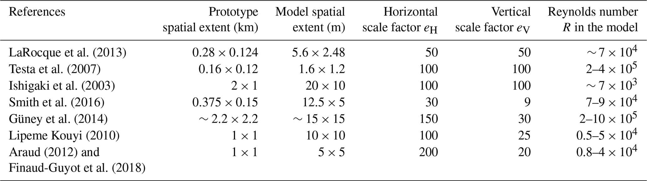
Table 1Recent laboratory experiments of urban flooding at the district level.
2.1 Undistorted and distorted models of urban flooding
Laboratory models have been used for studying urban flooding at various levels, ranging from limited spatial extents (e.g. a single storm drain) up to the level of a whole urban district. Some laboratory models focussing on a limited spatial extent were constructed at the prototype scale, i.e. with a scale factor equal to unity (Djordjevic et al., 2013; Lopes et al., 2013, 2017). At intermediate levels, such as when a single street or single crossroads are represented, scale factors of the order of 10–20 were used (Lee et al., 2013; Mignot et al., 2013; Rivière et al., 2011) which are generally deemed not to lead to excessive scale effects (Chanson, 2004). In contrast, when it comes to the experimental analysis of flooding at the level of an entire urban district, the spatial extent of the prototype to be represented becomes considerably larger (∼ 102–103 m), as summarized in Table 1 and sketched in Supplement 1, so that scale factors reach values as high as 100–200.
LaRocque et al. (2013) focussed on a limited portion of an urbanized floodplain (280 m × 124 m) and used a scale factor of 50, leading to a model Reynolds number of the order of . Testa et al. (2007) considered a scale factor of 100 for studying transient flooding of a group of buildings extending over 160 m × 120 m. This led nonetheless to model Reynolds numbers exceeding 105 because extreme flooding scenarios were tested (dam-break-induced flood). To analyse river flooding at the level of an entire urban district (1 km × 2 km), Ishigaki et al. (2003) also used a scale factor of 100; but in this case, despite a particularly large experimental facility (10 m × 20 m), the model Reynolds number was of the order of 7×10³, with water depth lower than 1 cm and being even lower than this amount in some streets. Ishigaki et al. (2003) reported that the observed flow became “laminar” in some parts of the model, hence exacerbating scale effects. This questions the validity of the upscaled lab observations and highlights a difficulty in the design of experimental models for analysing urban flooding, namely the substantial difference between the characteristic length in the horizontal direction (e.g. street width) and in the vertical direction (e.g. water depth). This issue is similar to the case of laboratory models of large rivers and coastal systems (Wakhlu, 1984).
To partly overcome this difficulty, so-called distorted laboratory models have also been used. They consist of applying distinct scale factors, respectively, eH and eV, along the horizontal and vertical directions:
where Hp and Hm are characteristic heights in the prototype and in the model, respectively. Since Lp is always much higher than Hp, using a horizontal scale factor eH larger than the vertical scale factor eV enables preserving higher water depths in the laboratory model compared to an equivalent undistorted model requiring the same horizontal space in the laboratory. This approach offers several advantages: (i) inaccuracies in water depth measurement become smaller in relative terms, and (ii) the Reynolds number is higher so that some artefacts (e.g. viscous effects) are minimized due to a change in the turbulence regime. By using a distorted model, it is even possible to keep both Reynolds and Froude numbers identical in the prototype and in the model, with the same fluid (Finaud-Guyot et al., 2018). Distorted models have been used for a broad range of applications in fluvial and coastal hydraulics. Among others, Jung et al. (2012) applied scale factors eH=120 and eV=50 to study a floating island in a river; Wakhlu (1984) obtained comparable results on an undistorted () and a distorted model (eH=100; eV=17) of a river division weir. However, since a distorted laboratory model corresponds to a representation of the prototype shrunk differently along the horizontal and the vertical directions, it may also lead to specific artefacts in the laboratory observations. For instance, Sharp and Khader (1984) highlighted distortion effects by comparing an undistorted () and a distorted model (eH=400; eV=100) to study wave transmission and assess stone stability in a harbour.
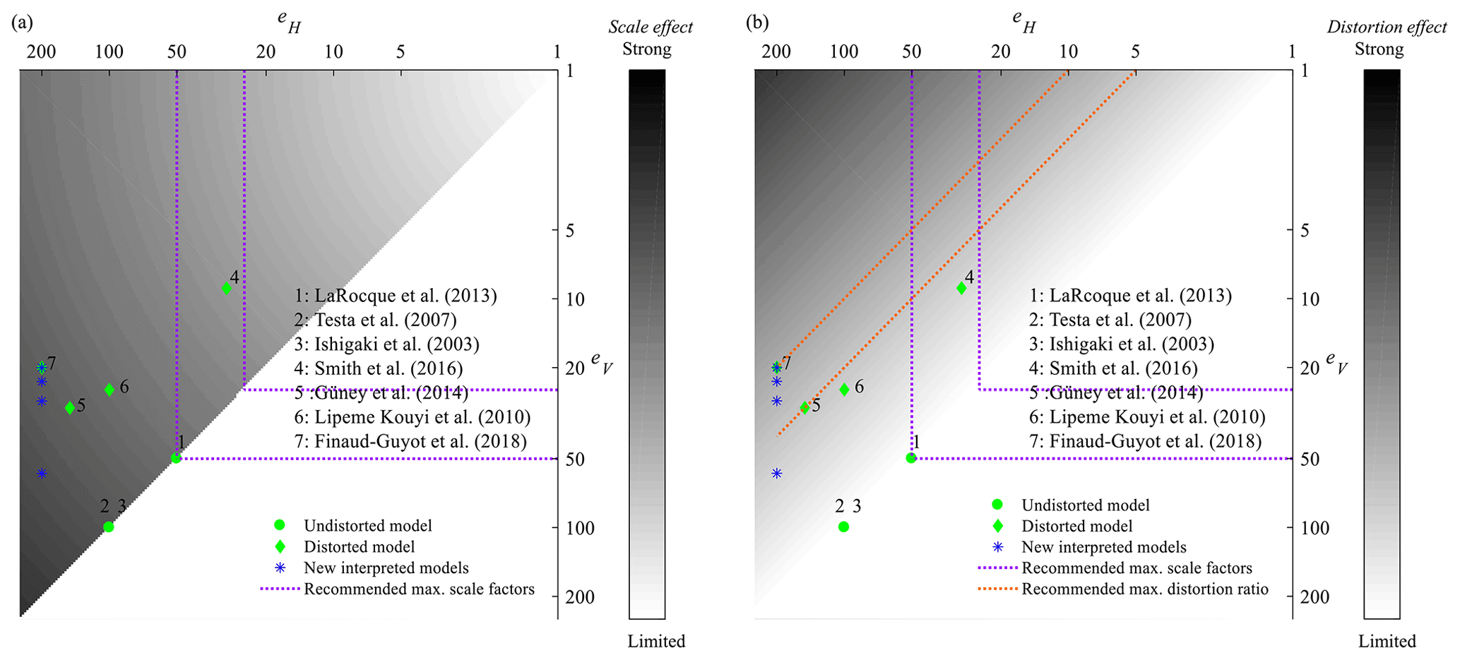
Figure 1Recent laboratory models of urban flooding at the district level as a function of the horizontal and vertical scale factors, eH and eV. The grey shading qualitatively reveals the possible magnitude of (a) scale effects and (b) distortion effects; a range of maximum scale factors (purple lines) and distortion ratio (orange lines) were recommended by Chanson (2004).
2.2 Recent studies based on distorted models of urban flooding and potential artefacts
Figure 1 shows the horizontal and vertical scale factors used in recent laboratory studies of urban flooding at the district level. The grey shading in Fig. 1a suggests conceptually that the larger the scale factors, the greater the expected scale effects, while Fig. 1b indicates that using a strongly distorted model (i.e. a large ratio eH∕eV) also leads to specific artefacts, which we refer to hereafter as distortion effects. Based on experience, Chanson (2004) suggests keeping the ratio eH∕eV below 5–10 (orange dotted lines in Fig. 1b).
An outdoor distorted model was used by Smith et al. (2016) to represent pluvial flooding in an urban district of relatively limited extent (Table 1). The scale factors were as low as eH=30 and eV=9 (distortion ratio: ), thus minimizing potential scale effects. Similarly, Güney et al. (2014) used an outdoor distorted model of a large urban district (Table 1), with eH=150 and eV=30 (distortion ratio: ), to represent dam-break-induced flood waves. The distortion ratio of these two models remains below the upper bound of 5–10, as recommended by Chanson (2004). Lipeme Kouyi et al. (2010), Araud (2012) and Finaud-Guyot et al. (2018) considered the same geometric configuration (Supplement 1) involving seven streets aligned along one direction, crossing seven other streets. The scale factors used by Lipeme Kouyi et al. (2010) were eH=100 and eV=25. The set-up of Araud (2012) and Finaud-Guyot et al. (2018) contains substantial improvements compared to the initial set-up of Lipeme Kouyi et al. (2010), mainly regarding the control of the inflow in each street separately, but it uses a considerably higher horizontal scale factor (eH=200) and, simultaneously, a smaller vertical scale factor (eV=20). This leads to a particularly high ratio eH∕eV, equal to the upper limit of 10 suggested by Chanson (2004). If the model of Araud (2012) and Finaud-Guyot et al. (2018) had not been distorted, the Reynolds numbers would have been about 30 times lower () than they actually are (Table 1).
2.3 Specific objective of the present study
While the motivations for using a large distortion ratio between the horizontal and vertical scale factors are not arguable (fit the model within a limited laboratory space, improve the accuracy of water depth measurement and maintain a sufficiently high Reynolds number), the assumption of having no artefacts in experimental observations performed on a strongly distorted model may legitimately be questioned. Among other aspects, the complex three-dimensional flow structures observed in individual crossroads (Mignot et al., 2008, 2013; Rivière et al., 2011, 2014) suggest that “shrinking” the model vertically is likely to alter these flow structures and hence also impair the representation of flow partition in-between the streets. The influence of strong distortion in laboratory-scale models was investigated for some specific applications, such as in coastal engineering (Ranieri, 2007; Sharp and Khader, 1984), but it has not been analysed to date in the context of laboratory models of urban flooding.
Therefore, in this paper, we aim to evaluate the artefacts arising from the use of distorted laboratory models in experimental studies of urban flooding at the district level. We base our assessment on the reanalysis of two recent datasets, presented, respectively, by Araud (2012) and by Velickovic et al. (2017). The latter does not represent a realistic urban district but solely a regular grid of obstacles, which is similar to a network of streets to some extent. We focus on the influence of model distortion on the observed water depths and discharge partition in-between the streets.
Table 2Initial interpretation of the laboratory model runs as various flooding scenarios represented with fixed scale factors (Araud, 2012; Finaud-Guyot et al., 2018) vs. interpretation in the present reanalysis, involving a single flood scenario represented with various vertical scale factors. Notations Qm and Qp refer to the total inflow in the laboratory model and in the prototype urban district, respectively.

3.1 Datasets
Two datasets were reanalysed, corresponding, respectively, to an entire urban district and to a group of buildings. The former dataset was collected by Araud (2012) in the ICube laboratory in Strasbourg (France) and was also presented by Arrault et al. (2016) and Finaud-Guyot et al. (2018) (Fig. S3a in Supplement 2). The experimental model (5 m × 5 m) represents an idealized urban district of 1 km × 1 km at the prototype scale. It contains a total of 14 streets of various widths (0.05–0.125 m) and 49 intersections (crossroads). The inflow discharge was controlled in each street individually, the uncertainty of the inflow discharge is estimated at about 1 % (Fiaud-Guyot et al., 2018) and the outflow discharges were monitored downstream of each street. The uncertainties in the estimation of the outflow discharges are discussed in Sect. 4.1. For several steady inflow discharges, the water depths along the centreline of streets were measured using an optical gauge (1 mm accuracy; Figs. S4–S7). Hereafter, we consider the experimental runs performed with a total inflow discharge Qm of 20, 60, 80 and 100 m3 h−1 in the laboratory model (Table 2). In each test, 50 % of the total inflow discharge was fed to the west face of the model and 50 % to the north face of the model. The specific inflow discharge was kept the same for each street of a given face, the outflow discharge was estimated from a calibrated rating curve (Araud, 2012). As detailed in Supplement 2–5, several measurements were repeated, which allows appreciating the reproducibility of the tests.
Table 3Interpretation of the dataset of Velickovic et al. (2017) in the present reanalysis. Notations Qm and Qp refer to the total inflow discharge in the laboratory model and in the prototype, respectively.
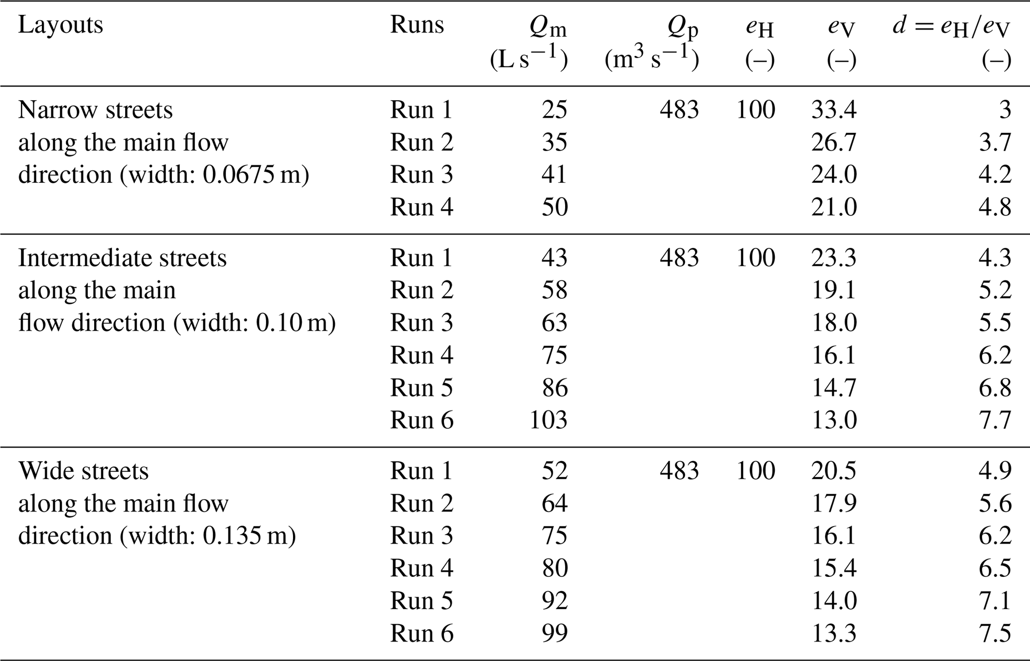
The second dataset was collected by Velickovic et al. (2017) in the Hydraulic Laboratory of Université Catholique de Louvain, Belgium. A group of 5×5 square obstacles (buildings) of 0.30 m × 0.30 m were installed in a horizontal flume 36 m × 3.6 m. Several layouts of obstacles were considered, and we analyse three of them here (aligned with the channel; Fig. S3b). For each of these layout, between four and six experimental runs (Table 3) were conducted with various steady inflow discharges (accuracy of flowmeters: ∼ 1 L s−1). The three layouts differ by the distance in-between the obstacles (i.e. the street widths) in the direction normal to the main flow (0.0675, 0.10 and 0.135 m). Profiles of water depth (accuracy: 0.1 mm) were measured with movable ultrasonic probes along the centreline of the streets aligned with the main flow direction. In contrast with the dataset of Araud (2012), the flow partition in-between the streets was not measured by Velickovic et al. (2017).
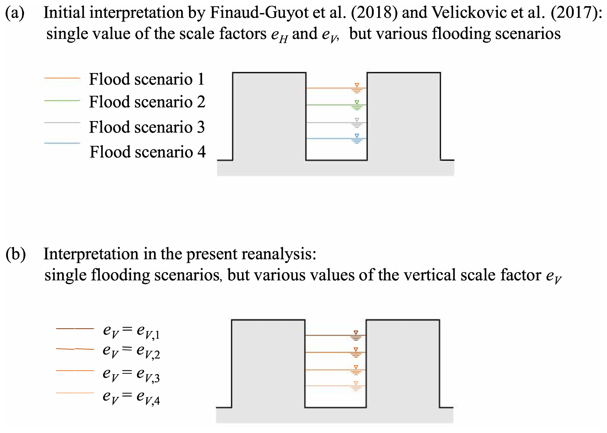
Figure 2(a) Sketch of the initial interpretation of the laboratory model runs as various flooding scenarios represented with fixed scale factors. (b) Sketch of the interpretation in the present reanalysis, involving a single flood scenario represented with various vertical scale factors eV.
3.2 Method
As sketched in Fig. 2a, the initial interpretation of the various experimental runs of Araud (2012) and Velickovic et al. (2017) was that each model run corresponds to a different flooding scenario (i.e. a different total inflow discharge Qm into the urban district) represented with fixed scale factors eH and eV. In contrast, in the present reanalysis of the laboratory dataset, we propose considering that a single flooding scenario was represented in each laboratory model but that the various experimental runs actually correspond to different vertical scale factors eV. This new perspective is sketched in Fig. 2b.
As detailed hereafter, we followed a three-step procedure for the reanalysis. For each model, the procedure was as follows:
-
Select one experimental run and assign to it plausible scale factors eH and eV.
-
Estimate the scale factor eV corresponding to each of the other experimental runs, assuming that eH remains unchanged and that all experimental runs simulate the same flood scenario.
-
Upscale the experimental observations of each run to the prototype scale and compare them to each other.
Step 1
We considered that Run 1 (Table 2) of Araud (2012) corresponds to a representation of a given flooding scenario in a strongly distorted scale model, consistent with the original values eH=200 and eV=20 reported by Arrault et al. (2016).
Similarly, for the dataset of Velickovic et al. (2017), we considered that the street width (0.10 m), in the model layout characterized by an intermediate street width, corresponds to 10 m in the prototype. This sets the horizontal scale factor to eH=100. Keeping eH=100 for the two other layouts leads to reproducing prototype street widths of 6.75 m for the narrow street layout and 13.5 m for the wide street layout. As shown in Table 3, we also assumed that the experimentally observed water depth (∼ 0.3 m) for the highest inflow discharge Qm in the layout with an intermediate street width (Run 6) corresponds to about 4 m in the prototype (i.e. extreme flooding conditions such as induced by a dam break). This leads to a vertical scale factor eV=13 for this run (Table 3).
Step 2
For the dataset of Araud (2012), Runs 2–4 in Table 2 are now assumed to represent the same flooding scenario as Run 1, with the same horizontal scale factor eH but with adjusted vertical scale factors eV. Similarly, all runs in Table 3 (dataset of Velickovic et al., 2017) represent the same flooding scenario as Run 6 of the intermediate street layout, but with different vertical scale factors. For both datasets, the adjusted values of eV were derived as follows:
-
The run selected in Step 1 was upscaled to the prototype scale, enabling the determination of the inflow discharge Qp in the prototype.
-
Knowing the inflow discharge Qm for each of the other model runs, the adjusted vertical scale factor was calculated as , consistent with Froude similarity.
The values of eV derived from this procedure are detailed in Tables 2 and 3 for the two datasets. The model distortion, expressed as the ratio d between eH and eV, varies from 3 to 7.7 in the dataset of Velickovic et al. (2017) and from 3.4 to 10 in the dataset of Araud (2012).
Step 3
Finally, for each model, the experimental observations of all model runs (measured water depths and outflow discharges) were upscaled to the prototype scale and compared. This approach is similar to the “scale series” method described by Heller (2011) and used by Erpicum et al. (2016), although here we vary only the vertical scale factor.
If there were no artefacts arising from the model distortion, the prototype scale predictions from the different experimental runs should superimpose. In the following, we assess the magnitude of the distortion effects by comparing the upscaled observations from each experimental run with one selected reference, namely the experimental run corresponding to the weakest distortion (minimum value of d), for which we have the highest confidence in prototype event replication: Run 4 (d=3.4) in the dataset of Araud (2012) and Run 1 of each layout (d=3, 4.3, 4.9) in the dataset of Velickovic et al. (2017).
We first present an estimation of the experimental uncertainties (Sect. 4.1); then, we detail the effect of model distortion on the upscaled water depths (Sect. 4.2). Finally, we present the effect of model distortion on the partition of outflow discharges (Sect. 4.3).
4.1 Experimental uncertainties
The measurement accuracy and the fluctuations of water surface are considered the two main sources of uncertainty in the experimental records of water depths. For the dataset of Araud (2012), the accuracy of the optical gauge is about 1 mm. As shown in Supplement 2, the water depths were measured twice at some locations for Run 3 (60 m3 h−1) and Run 2 (80 m3 h−1). The repeatability of the tests is evaluated by comparing the repeated measurements. As detailed in Supplement 3, the difference in water depths between two measurements remains below 2 mm for 90 % of the dataset. Therefore, we estimate here the water depth measurement uncertainty at about 2 mm. Representative profiles of measured water depths (including repetitions) are displayed in Supplement 4, and they confirm the validity of this uncertainty estimate. Uncertainties arising from inaccuracies in the inflow discharge measurement are also lumped into this uncertainty estimate.
The discharge at the outlet of each street was estimated from a rating curve corresponding to a weir at the downstream end of dedicated measurement channels (located downstream of each street outlet). The water depth measurements were performed at least three times for each model run. As detailed in Supplement 5, comparing the repeated measurements demonstrates an excellent repeatability of the outflow discharge estimates (Figs. S12–S15). Hence, the main source of uncertainty in the outflow discharge estimates is assumed to stem from the accuracy of water depth measurement (1 mm) over the measurement weirs (Araud, 2012). This leads to about 2 %–6 % uncertainty in the outflow discharges, as shown in Fig. S16.

Figure 3Upscaled water depth profiles in prototype in street 4 of Araud (2012) predictions, colour shade represents the upscaled measurement uncertainty.
For the second dataset, the accuracy of the probes, as described by Velickovic et al. (2017), is 0.1 mm. Velickovic et al. (2017) also reported the standard deviation of the recorded water depths at each probe location. We used this as a proxy for estimating the flow variability. Figure S9 in Supplement 3 shows the cumulative distribution function of this standard deviation over all measured data in the three layouts and for each experimental run. For 90 % of the measurement points, the standard deviation remains below 2–6 mm (depending on the experimental run), which reflects considerable fluctuations in the free surface, particularly for the higher flow rates.
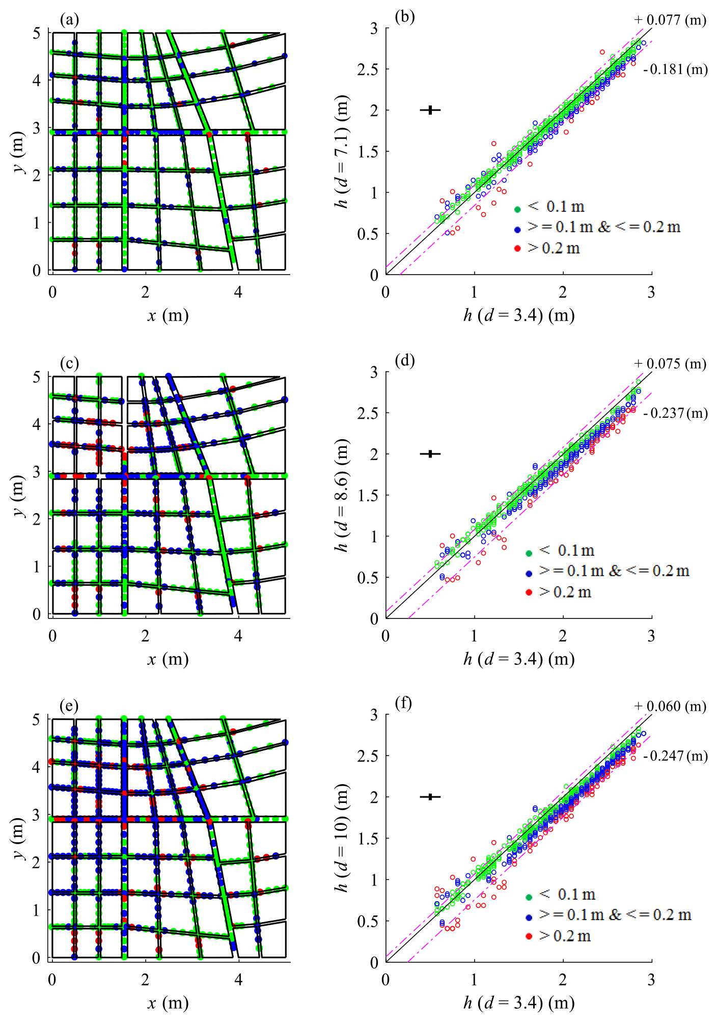
Figure 4Spatial distributions (a, c, e) and scatter plots (b, d, f) of the differences between the upscaled water depths in Run 3 (d=7.1), 2 (d=8.6) and 1 (d=10), and those derived from Run 4 (d=3.4) from Araud (2012). The dashed purple lines indicate the range containing 90 % of the data.
4.2 Effect of model distortion on predicted water depths
4.2.1 Dataset of Araud (2012)
All measured water depths were upscaled to the prototype scale using the vertical scale factors defined in Table 2. As exemplified in Fig. 3 for street 4 (and in Figs. S17 and S18 in Supplement 6 for streets A, B, and C), the tests conducted with the strongest distortion (d=8.6 and d=10) lead to the lowest estimates of water depths at the prototype scale. Conversely, the highest predicted water depths correspond systematically to the upscaled measurements from the tests involving a weaker distortion (d=3.4), except nearby the downstream boundary conditions where all predicted water depths are close to each other. The tests conducted with d=7.1 lead to intermediate estimates of water depths at the prototype scale. The reasons for these differences are discussed in Sect. 5.1. Here, the uncertainty associated to the upscaled water depths is larger when the model distortion is limited, since the absolute value of the measurement uncertainty remains the same in all model runs, but a larger vertical scale factor is applied.
Table 4Differences between upscaled water depths derived from various runs of Araud (2012).
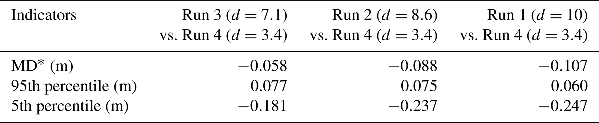
∗ MD stands for mean difference.
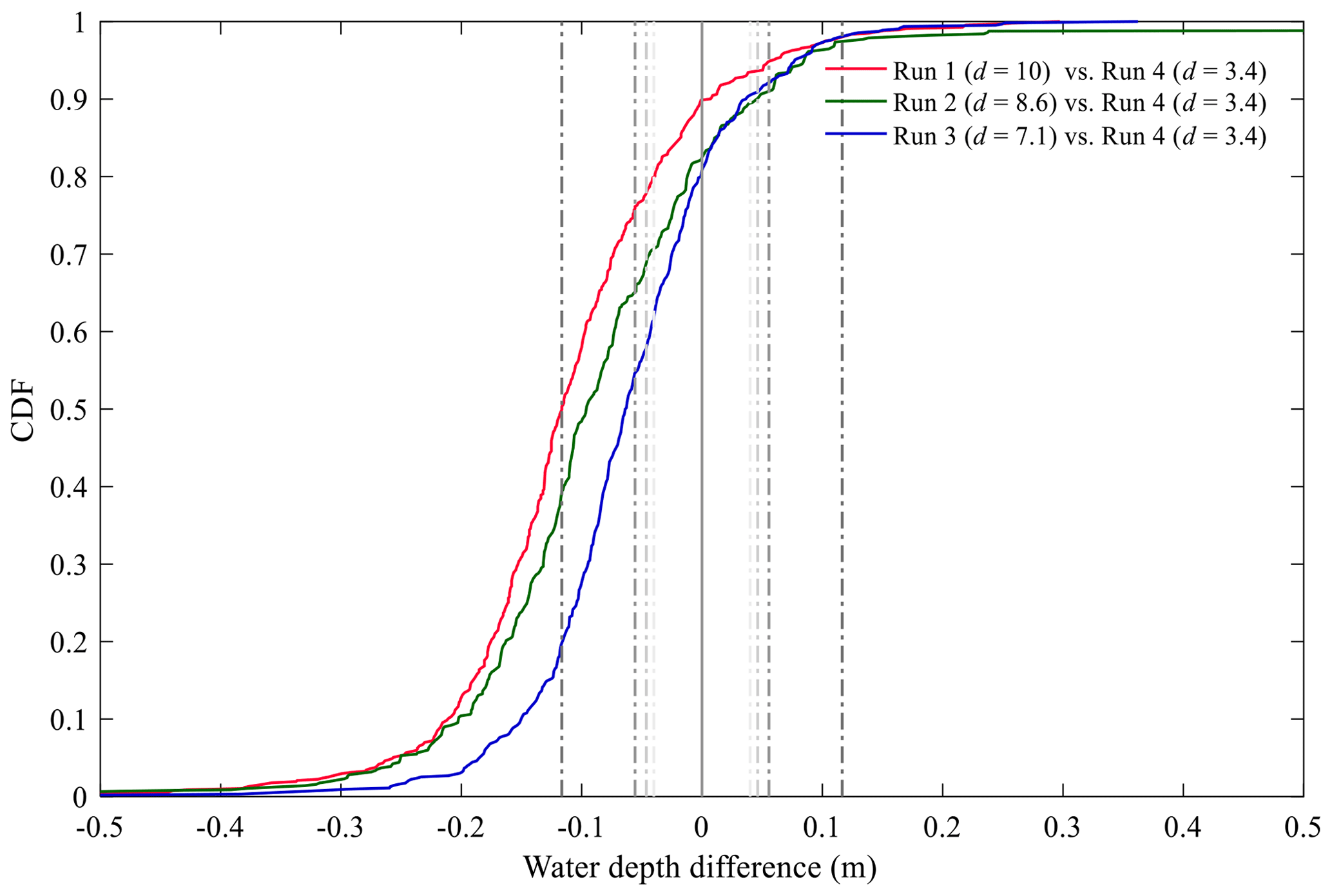
Figure 5Cumulative distribution function (CDF) of the differences between upscaled water depths from the various model runs of Araud (2012); the grey lines represent the upscaled measurement uncertainties with various eV (the larger the eV, the deeper the line colour).
In Figs. 4 and 5 and Table 4, we quantitatively compare the upscaled water depths obtained from the four different model runs listed in Table 2. The model run with the weakest distortion is used as a reference for comparisons. The following observations can be made:
-
The scatter plots in Fig. 4 confirm that the water depths derived from the model with the lowest distortion are generally higher than those derived from the other model runs.
-
The dashed purple lines (and corresponding labels; Fig. 4b, d, f) indicate the range containing 90 % of the data. This shows that, despite the uncertainties in the measurements, the differences between the model runs increase very consistently as the model distortion increases. This consistent trend is also emphasized by the evolution of the mean difference (MD in Table 4) from −0.058 to −0.107 as d varies from 7.1 to 10 as well as by the cumulative distribution of the differences in upscaled water depths derived from the various model runs (Fig. 5).
-
The 5th percentile of the differences between the models with varying distortions is of the order of −20 to −25 cm (Table 4). When compared to the order of magnitude of the absolute value of water depths (∼ 2 m), the effect of model distortion in the tested configurations is of the order of 10 % of the upscaled water depths.
-
The spatial distributions provided in Fig. 4 also reveal that the influence of model distortion tends to increase in the upstream part of the urban district (i.e. closer to the north and west faces). Two reasons contribute to explain this: (i) the water depths in the downstream part are mainly controlled by the free outflow boundaries and remain therefore more similar whatever the distortion; and (ii) the cumulated effect of friction (expected to be underestimated in the more distorted models compared to the less distorted or undistorted models, as detailed in Sect. 5.1) is stronger in the upstream part of the flow.
Table 5Differences between upscaled water depths derived from various runs of Velickovic et al. (2017).
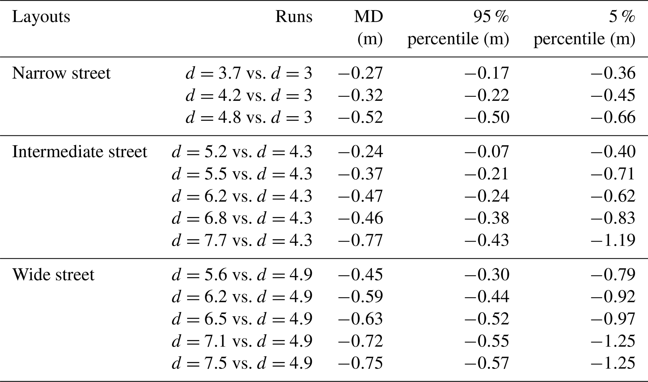
∗ MD stands for mean difference.
4.2.2 Dataset of Velickovic et al. (2017)
Figure S19 in Supplement 7 displays the upscaled water depth profiles based on the dataset of Velickovic et al. (2017) and the scale factors defined in Table 3 for each of the three layouts. The upscaled water depths in the three model layouts differ substantially as the same discharge Qp is imposed (hp in narrow street: ∼ 5 m; median street: ∼ 3.5 m; wide street: ∼ 2.5 m). Now, for each model layout separately, we compare the observations corresponding to various inflow discharges in the same way as in the dataset of Araud (2012). It is found that the upscaled water depths in the urban area become systematically lower as the model distortion increases. This is observed consistently for the three layouts of obstacles (narrow, intermediate and wide streets), and the differences arising from the change in model distortion greatly exceed the estimated experimental uncertainty. This result is also confirmed by the values of mean differences (MDs) reported in Table 5 as well as by the cumulative distribution functions of the differences in water depths (Fig. S20 in Supplement 7). In each layout, the model characterized by the lowest value of d was taken as a reference for comparison.
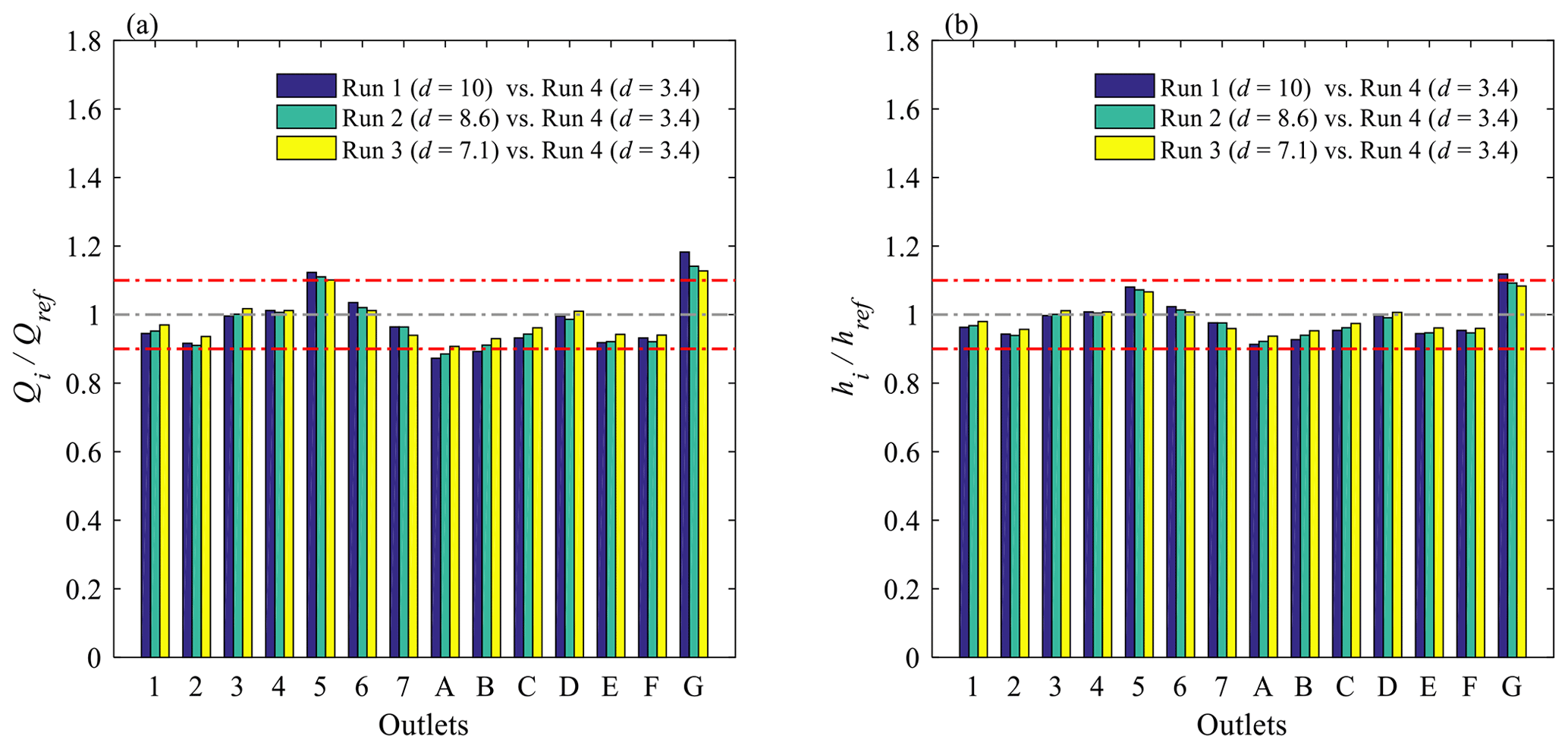
Figure 6(a) Upscaled outflow discharge in each street compared to the corresponding value deduced from the observations in the less distorted model (d=3.4), and (b) ratio of the associated water depths from Araud (2012) and Finaud-Guyot et al. (2018). Red dashed lines represent the ±10 % range.
4.3 Effect of model distortion on outflow discharges
For the dataset of Araud (2012), the upscaled values of the discharge at the outlet of each street are shown in Supplement 8 (Fig. S21). Although the differences in the outflow discharge appear to be of the same order of magnitude as the experimental uncertainties, the variation in the outflow discharge partition with d shows a consistent monotonous trend (increasing, constant or decreasing) in all outlet streets. Since the mass balance remains unchanged at the level of the whole district, the direction of change in the outlet discharge varies from one street to the other. In Fig. 6a, we compare the upscaled outflow discharge in each street to the corresponding value derived from the less distorted model (d=3.4). The changes in the estimated outflow discharge when d is varied are in the range of ±10 % in 11 streets out of 14 (and are in the range of ±12 % in 13 streets out of 14, with a maximum change of +18 % in just a single street).
The magnitude of model distortion effects may differ from one flow variable to the other (Heller, 2011). To be able to appreciate the relative influence of model distortion on the outflow discharge and on the water depths, for each street outlet (noted i), we estimated the change in upscaled water depth (hi∕href) “associated” with the observed change in the outflow discharge (Qi∕Qref) when the model distortion is varied (from dref to di). To do so, using Froude similarity leads to . As shown in Fig. 6, the results indicate that, in the present case, the magnitude of model distortion effects appears to be relatively comparable for the water depths and the outflow discharges (of the order of ±10 %).
5.1 Relative importance of the main causes of distortion effects
The differences in the upscaled water depths as a function of the model distortion d may result from differences in localized flow features (e.g. local head losses at street intersections) and from more distributed effects, which in the present case are likely to dominate only along the mainly one-dimensional flow regions (typically within a street). The latter effects may be categorized into three types:
-
differences in the relative importance of the bottom roughness,
-
differences in the relative importance of viscosity effects,
-
differences in the aspect ratio (ratio between water depth and street width) of the flow section, notably affecting the secondary currents and velocity profiles of streamline velocity.
It is possible that the third of these effects has a substantial influence on the flow. However, the available datasets, involving only observed water depths and discharges at the model outlets, do not enable investigating these more localized effects in detail. This could be achieved by means of new experiments with detailed velocity measurements within the urban district. 2-D and 3-D computational modelling may also be useful in this respect, the former enabling us to account for the spatial variations of flow characteristics and the latter giving us full access to the complex flow fields developing at the street intersections.
Nonetheless, we appreciate here the influence of the first two types of effects, which are of relevance to mainly one-dimensional flow regions. To do so, we estimate the energy slope Sf,p at the prototype scale in the various model configurations based on the Darcy–Weisbach equation.
In this equation, the friction coefficient fm can be computed as a function of the Reynolds number Rm and the relative roughness height using the explicit approximation of the Colebrook–White formula given by Yen (2002). The roughness height ks,m was taken to be equal to 10−5 m to represent the smooth bottom and walls of the experimental set-ups.

Figure 7Distortion effect on energy slope of (a) scale models and (b) the model in prototype (dataset of Araud, 2012).
Figure S22 shows the values of parameters Rm, , fm, , and F, which are representative of the flow conditions at the street inlets in the various experimental runs of Araud (2012). Given the values of Rm and , the flow is in a transitional regime in the Moody diagram. All these parameters change substantially when the model distortion d is varied (Fig. S23). As d is increased, the friction coefficient fm decreases systematically () due to the joint effect of a higher Reynolds number and a lower relative roughness height (). Similarly, the Froude number tends to slightly increase with the model distortion. In contrast, parameter shows a considerable systematic increase (1.6–2.3) as d increases due to the change in the aspect ratio of the flow section. The resulting energy slope Sf,m in the inlet streets in each model run and the corresponding upscaled values Sf,p are presented in Fig. 7. The energy slope is lower in major streets (4, C, F) and in the straight streets (A, B). The energy slope Sf,m in the model increases monotonously with the model distortion (mainly due to the increased wetted perimeter), whereas the energy slope Sf,p at the prototype scale declines as d is increased (Fig. 7b). This results from a “competition” between the increase in Sf,m and a decrease in the ratio eV∕eH, as d increases. This effect appears dominant in the mainly one-dimensional flow regions.
5.2 Reference used for comparison
Here, we used the “less distorted” models as a reference for our comparisons since the aim is to assess the influence of model distortion. However, given that we simply reanalysed already existing datasets obtained in experiments which were not designed for the sake of investigating the effect of model distortion in the first place, these less distorted models are also those characterized by the largest vertical scale factors, hence enhancing other artefacts such as stronger viscosity effects (see asterisks in Fig. 1). Also, the upscaled measurement uncertainties are at a maximum in this case, as can be seen in Fig. 3. Therefore, the present study needs to be complemented by new tailored experiments involving a model series (Heller, 2011) with various levels of distortion and including a valid reference model, i.e. at least one model without distortion and that is characterized by sufficiently small scale factors so that viscosity effects and experimental uncertainties are kept to a minimum. This may be achieved by considering a model series in which the vertical scale factor eV is kept constant in all models, while only the horizontal scale factor eH is varied. This approach contrasts with the procedure followed here in which eH was constant and eV was varied to take benefit of existing datasets.
Laboratory-scale models representing flooding of an entire urban district are usually distorted, in the sense that the vertical scale factor (Hp∕Hm) is often considerably smaller than the horizontal one. This paper evaluates the influence of the model distortion on the upscaled values of water depths and outflow discharge for relatively extreme flood conditions (water depth and flow velocity of the order of 1–2 m and 0.5–2 m s−1 at the prototype scale). Two existing experimental datasets were reanalysed for this purpose. The results show that the stronger the model distortion, the lower the values of the upscaled water depths, whereas the influence on flow partition at the outlet of the street appears more complex.
The change in the upscaled water depths was found to be of the order of 10 % when the distortion of the model was varied by a factor of 3. Moreover, a deviation of about 10 % was also obtained for the outflow discharges. This is of the same order as the influence of small-scale obstacles, as reported by Bazin et al. (2017).
For the water depths, the effect of varying the model distortion was found to be generally larger than the measurement uncertainties, whereas both effects are comparable for the discharge at the street outlets in the tested configurations. Note that the relative measurement uncertainties are smaller in distorted models than in undistorted models.
The uncertainty in the upscaled water depths is considerably larger in the models with limited distortion, because they also correspond to the highest vertical scale factors. Using those results as a reference seems sensible for assessing the effect of distortion since they correspond to the lowest values of d, but at the same time it is somehow problematic to use the results with the highest uncertainty as a reference (e.g. Figs. S17–S18). To overcome this issue, future experimental research should involve “model series” in which the horizontal scale factor eH is reduced without changing the vertical scale factor eV. This will enable the reduction of the influence of distortion without increasing the error in the estimated water depths, but this requires the collection of new experimental measurements which are presently lacking.
This study is a contribution towards a deeper understanding of small-scale flow processes which govern urban flooding and need to be incorporated in urban hydrological models, either explicitly or through parametrization. In future, more controlling parameters should also be considered, such as the bottom slope, and computational modelling should complement the laboratory experiments (e.g. Ichiba et al., 2018; Ozdemir et al., 2013). Moreover, in real-world urban flooding, the urban drainage system may also have a substantial influence. Laboratory modelling of dual drainage becomes even more intricate due to the combination of pressurized and surface flow (e.g. Rubinato et al., 2017). This poses additional constraints on the design of the scale models and leads to extra experimental challenges which deserve further research. Finally, existing experiments of urban flooding at the district level have delivered mostly discharge and water depth data, but there is a need for more pointwise velocity measurements (e.g. Martins et al., 2018) to gain deeper insights into the flow processes.
The data presented in this paper can be accessed from the dataset listed in the references (Li et al., 2019).
The supplement related to this article is available online at: https://doi.org/10.5194/hess-23-1567-2019-supplement.
XL conducted the analysis and wrote the first version of the paper, which was revised by BD. PA and BD formulated the research question. PFG shared the ICube experimental data and, together with MB, helped with the analysis and interpretation of the dataset. BD, EM, SE, PA and MP supported the analysis and interpretation of the results. All co-authors revised successive versions of the paper.
The authors declare that they have no conflict of interest.
This research was partly funded through a grant for Concerted Research
Actions (grant no. ARC 13-17/01) financed by the Wallonia-Brussels
Federation,
and it also benefitted from the support of French Community of Belgium with the
financing of FRIA grant. The authors gratefully acknowledge Sandra
Soares-Frazão (Université Catholique de Louvain, Belgium) for sharing
the experimental datasets.
Edited by:
Marie-Claire ten Veldhuis
Reviewed by: two anonymous referees
Araud, Q.: Simulation des écoulements en milieu urbain lors d'un événement pluvieux extrême, Université de Strasbourg, 2012.
Arrault, A., Finaud-Guyot, P., Archambeau, P., Bruwier, M., Erpicum, S., Pirotton, M., and Dewals, B.: Hydrodynamics of long-duration urban floods: experiments and numerical modelling, Nat. Hazards Earth Syst. Sci., 16, 1413–1429, https://doi.org/10.5194/nhess-16-1413-2016, 2016.
Bazin, P.-H., Mignot, E., and Paquier, A.: Computing flooding of crossroads with obstacles using a 2-D numerical model, J. Hydraul. Res., 55, 72–84, https://doi.org/10.1080/00221686.2016.1217947, 2017.
Brown, R. and Chanson, H.: Suspended sediment properties and suspended sediment flux estimates in an inundated urban environment during a major flood event, Water Resour. Res., 48, W11523, doi:10.1029/2012WR012381, 2012.
Brown, R. and Chanson, H.: Turbulence and suspended sediment measurements in an urban environment during the Brisbane River flood of january 2011, J. Hydraul. Eng., 139, 244–253, https://doi.org/10.1061/(ASCE)HY.1943-7900.0000666, 2013.
Chanson, H.: 14 – Physical modelling of hydraulics, in: Hydraulics of Open Channel Flow (Second Edition), edited by: Chanson, H., 253–274, Butterworth-Heinemann, Oxford, 2004.
Chen, Y., Zhou, H., Zhang, H., Du, G., and Zhou, J.: Urban flood risk warning under rapid urbanization, Environ. Res., 139, 3–10, https://doi.org/10.1016/j.envres.2015.02.028, 2015.
Djordjevic, S., Saul, A. J., Tabor, G. R., Blanksby, J., Galambos, I., Sabtu, N., and Sailor, G.: Experimental and numerical investigation of interactions between above and below ground drainage systems, Water Sci. Technol., 67, 535–542, https://doi.org/10.2166/wst.2012.570, 2013.
Dottori, F., Di Baldassarre, G., and Todini, E.: Detailed data is welcome, but with a pinch of salt: Accuracy, precision, and uncertainty in flood inundation modeling, Water Resour. Res., 49, 6079–6085, 2013.
Dottori, F., Figueiredo, R., Martina, M. L. V., Molinari, D., and Scorzini, A. R.: INSYDE: a synthetic, probabilistic flood damage model based on explicit cost analysis, Nat. Hazards Earth Syst. Sci., 16, 2577–2591, https://doi.org/10.5194/nhess-16-2577-2016, 2016.
Erpicum, S., Tullis, B. P., Lodomez, M., Archambeau, P., Dewals, B. J., and Pirotton, M.: Scale effects in physical piano key weirs models, J. Hydraul. Res., 54, 692–698, https://doi.org/10.1080/00221686.2016.1211562, 2016.
Finaud-Guyot, P., Garambois, P.-A., Araud, Q., Lawniczak, F., François, P., Vazquez, J., and Mosé, R.: Experimental insight for flood flow repartition in urban areas, Urban Water J., 15, 242–250, https://doi.org/10.1080/1573062X.2018.1433861, 2018.
Gaines, J. M.: Flooding: Water potential, Nature, 531, 54–55, 2016.
Güney, M. S., Tayfur, G., Bombar, G., and Elci, S.: Distorted Physical Model to Study Sudden Partial Dam Break Flows in an Urban Area, J. Hydraul. Eng., 140, 05014006, https://doi.org/10.1061/(ASCE)HY.1943-7900.0000926, 2014.
Heller, V.: Scale effects in physical hydraulic engineering models, J. Hydraul. Res., 49, 293–306, https://doi.org/10.1080/00221686.2011.578914, 2011.
Heller, V., Hager, W. H., and Minor, H.-E.: Scale effects in subaerial landslide generated impulse waves, Exp. Fluids, 44, 691–703, https://doi.org/10.1007/s00348-007-0427-7, 2008.
Hettiarachchi, S., Wasko, C., and Sharma, A.: Increase in flood risk resulting from climate change in a developed urban watershed – the role of storm temporal patterns, Hydrol. Earth Syst. Sci., 22, 2041–2056, https://doi.org/10.5194/hess-22-2041-2018, 2018.
Ichiba, A., Gires, A., Tchiguirinskaia, I., Schertzer, D., Bompard, P., and Ten Veldhuis, M.-C.: Scale effect challenges in urban hydrology highlighted with a distributed hydrological model, Hydrol. Earth Syst. Sci., 22, 331–350, https://doi.org/10.5194/hess-22-331-2018, 2018.
Ishigaki, T., Keiichi, T., and Kazuya, I.: Hydraulic model tests of inundation in urban area with underground space, Theme B, Proc. of XXX IAHR Cogress, Greece, available from: https://ci.nii.ac.jp/naid/10029665177/en/, 487–493, 2003.
Jung, S., Kang, J., Hong, I., and Yeo, H.: Case study: Hydraulic model experiment to analyze the hydraulic features for installing floating islands, Sci. Res., 4, 90–99, https://doi.org/10.4236/eng.2012.42012, 2012.
Kreibich, H., Van Den Bergh, J. C. J. M., Bouwer, L. M., Bubeck, P., Ciavola, P., Green, C., Hallegatte, S., Logar, I., Meyer, V., Schwarze, R., and Thieken, A. H.: Costing natural hazards, Nat. Clim. Change, 4, 303–306, 2014.
LaRocque, L. A., Elkholy, M., Chaudhry, M. H., and Imran, J.: Experiments on Urban Flooding Caused by a Levee Breach, J. Hydraul. Eng., 139, 960–973, https://doi.org/10.1061/(ASCE)HY.1943-7900.0000754, 2013.
Lee, S., Nakagama, H., Kawaike, K., and Zhang, H.: Experimental validation pf interaction model at storm drain for development of intergrated urbain inundation model, J. Jpn. Soc. Lubr. Eng., 69, 109–114, https://doi.org/10.2208/jscejhe.69.I_109, 2013.
Lehmann, J., Coumou, D., and Frieler, K.: Increased record-breaking precipitation events under global warming, Clim. Change, 132, 501–515, https://doi.org/10.1007/s10584-015-1434-y, 2015.
Li, X., Erpicum, S., Bruwier, M., Mignot, E., Finaud-Guyot, P., Archambeau, P., Pirotton, M., and Dewals, B.: Supporting data for: “Laboratory modelling of urban flooding: strengths and challenges of distorted scale models” (Data set), https://doi.org/10.5281/zenodo.2586900, 2019.
Lipeme Kouyi, G., Rivière, N., Vidalat, V., Becquet, A., Chocat, B., and Guinot, V.: Urban flooding: One-dimensional modelling of the distribution of the discharges through cross-road intersections accounting for energy losses, Water Sci. Technol., 61, 2021–2026, https://doi.org/10.2166/wst.2010.133, 2010.
Liu, D.: Water supply: China's sponge cities to soak up rainwater, Nature, 537, 307, https://doi.org/10.1038/537307c, 2016.
Lopes, P., Leandro, J., Carvalho, R. F., Pascoa, P., and Martins, R.: Numerical and experimental investigation of a gully under surcharge conditions, Urban Water J., 12, 468–476, https://doi.org/10.1080/1573062X.2013.831916, 2013.
Lopes, P., Carvalho, R. F., and Leandro, J.: Numerical and experimental study of the fundamental flow characteristics of a 3-D gully box under drainage, Water Sci. Technol., 75, 2204–2215, https://doi.org/10.2166/wst.2017.071, 2017.
Mallakpour, I. and Villarini, G.: The changing nature of flooding across the central United States, Nat. Clim. Change, 5, 250–254, https://doi.org/10.1038/nclimate2516, 2015.
Martins, R., Rubinato, M., Kesserwani, G., Leandro, J., Djordjevic, S., and Shucksmith, J. D.: On the Characteristics of Velocities Fields in the Vicinity of Manhole Inlet Grates During Flood Events, Water Resour. Res., 54, 6408–6422, https://doi.org/10.1029/2018WR022782, 2018.
Mignot, E., Paquier, A., and Rivière, N.: Experimental and numerical modeling of symmetrical four-branch supercritical cross junction flow, J. Hydraul. Res., 46, 723–738, https://doi.org/10.3826/jhr.2008.2961, 2008.
Mignot, E., Zeng, C., Dominguez, G., Li, C.-W., Rivière, N., and Bazin, P.-H.: Impact of topographic obstacles on the discharge distribution in open-channel bifurcations, J. Hydrol., 494, 10–19, https://doi.org/10.1016/j.jhydrol.2013.04.023, 2013.
Mignot, E., Li, X., and Dewals, B.: Experimental modelling of urban flooding: A review, J. Hydrol., 568, 334–342, https://doi.org/10.1016/j.jhydrol.2018.11.001, 2019.
Molinari, D. and Scorzini, A. R.: On the influence of input data quality to Flood Damage Estimation: The performance of the INSYDE model, Water, 9, 688, https://doi.org/10.3390/w9090688, 2017.
Moy de Vitry, M., Dicht, S., and Leitão, J. P.: floodX: urban flash flood experiments monitored with conventional and alternative sensors, Earth Syst. Sci. Data, 9, 657–666, https://doi.org/10.5194/essd-9-657-2017, 2017.
Novak, P.: Scaling Factors and Scale Effects in Modelling Hydraulic Structures, in: Symposium on Scale Effects in Modelling Hydraulic Structures, edited by: Kobus, H., International Association for Hydraulic Reasearch (IAHR), 0.3–1–0.3–5, 1984.
Ozdemir, H., Sampson, C. C., de Almeida, G. A. M., and Bates, P. D.: Evaluating scale and roughness effects in urban flood modelling using terrestrial LIDAR data, Hydrol. Earth Syst. Sci., 17, 4015–4030, https://doi.org/10.5194/hess-17-4015-2013, 2013.
Park, H., Cox, D. T., Lynett, P. J., Wiebe, D. M., and Shin, S.: Tsunami inundation modeling in constructed environments: A physical and numerical comparison of free-surface elevation, velocity, and momentum flux, Coast. Eng., 79, 9–21, https://doi.org/10.1016/j.coastaleng.2013.04.002, 2013.
Ranieri, G.: The surf zone distortion of beach profiles in smalle-scale coastal models, J. Hydraul. Res., 45, 261–269, https://doi.org/10.1080/00221686.2007.9521761, 2007.
Rivière, N., Travin, G., and Perkins, R. J.: Subcritical open channel flows in four branch intersections, Water Resour. Res., 47, W10517, https://doi.org/10.1029/2011WR010504, 2011.
Rivière, N., Travin, G., and Perkins, R. J.: Transcritical flows in three and four branch open-channel intersections, J. Hydraul. Eng., 140, 04014003, https://doi.org/10.1061/(ASCE)HY.1943-7900.0000835, 2014.
Rubinato, M., Martins, R., Kesserwani, G., Leandro, J., Djordjevic, S., and Shucksmith, J.: Experimental calibration and validation of sewer/surface flow exchange equations in steady and unsteady flow conditions, J. Hydrol., 552, 421–432, https://doi.org/10.1016/j.jhydrol.2017.06.024, 2017.
Sharp, J. J. and Khader, M. H. A.: Scale effects in Harbour Models Invovling Permeable Rubble Mound Structures, in: Symposium on Scale Effects in Modelling Hydraulic Structures, edited by: Kobus, H., International Association for Hydraulic Reasearch (IAHR), 7.12-1–.12–5, 1984.
Smith, G. P., Rahman, P. F., and Wasko, C.: A comprehensive urban floodplain dataset for model benchmarking, International Journal of River Basin Management, 14, 345–356, https://doi.org/10.1080/15715124.2016.1193510, 2016.
Testa, G., Zuccala, D., Alcrudo, F., Mulet, J., and Soares-Frazão, S.: Flash flood flow experiment in a simplified urban district, J. Hydraul. Res., 45, 37–44, https://doi.org/10.1080/00221686.2007.9521831, 2007.
UNISDR: The human cost of weather related disasters, CRED 1995–2015, United Nations, Geneva, 2015.
Velickovic, M., Zech, Y., and Soares-Frazão, S.: Steady-flow experiments in urban areas and anisotropic porosity model, J. Hydraul. Res., 55, 85–100, https://doi.org/10.1080/00221686.2016.1238013, 2017.
Wakhlu, O. N.: Scale Effects in Hydraulic Model Studies, in: Symposium on Scale Effects in Modelling Hydraulic Structures, edited by: Kobus, H., International Association for Hydraulic Reasearch (IAHR), 2.13-1–2.13-6, 1984.
Wright, N.: Advances in flood modelling helping to reduce flood risk, Proceedings of the Institution of Civil Engineers: Civil Engineering, 167, 52–52, https://doi.org/10.1680/cien.2014.167.2.52, 2014.
Yen, B. C.: Open channel flow resistance, J. Hydraul. Eng., 128, 20–39, 2002.
Zhou, Q., Leng, G., and Huang, M.: Impacts of future climate change on urban flood volumes in Hohhot in northern China: benefits of climate change mitigation and adaptations, Hydrol. Earth Syst. Sci., 22, 305–316, https://doi.org/10.5194/hess-22-305-2018, 2018.
Zhou, Q., Yu, W., Chen, A. S., Jiang, C., and Fu, G.: Experimental Assessment of Building Blockage Effects in a Simplified Urban District, Procedia Engineer., 154, 844–852, 2016.