the Creative Commons Attribution 4.0 License.
the Creative Commons Attribution 4.0 License.
 | 21 Mar 2019
Precipitation projections using a spatiotemporally distributed method: a case study in the Poyang Lake watershed based on the MRI-CGCM3
Ling Zhang
Xiaoling Chen
Xiaokang Fu
Yufang Zhang
Dong Liang
Qiangqiang Xu
To bridge the gap between large-scale GCM (global climate model) outputs and regional-scale climate requirements of hydrological models, a spatiotemporally distributed downscaling model (STDDM) was developed. The STDDM was done in three stages: (1) up-sampling grid-observations and GCM simulations for spatially continuous finer grids, (2) creating the mapping relationship between the observations and the simulations differently in space and time, and (3) correcting the simulation and producing downscaled data to a spatially continuous grid scale. We applied the STDDM to precipitation downscaling in the Poyang Lake watershed using the MRI-CGCM3 (Meteorological Research Institute Coupled Ocean–Atmosphere General Circulation Model 3), with an acceptable uncertainty of ≤ 4.9 %. Then we created future precipitation changes from 1998 to 2100 (1998–2012 in the historical scenario and 2013–2100 in the RCP8.5 scenario). The precipitation changes increased heterogeneities in temporal and spatial distribution under future climate warming. In terms of temporal patterns, the wet season become wetter, while the dry season become drier. The frequency of extreme precipitation increased, while that of the moderate precipitation decreased. Total precipitation increased, while rainy days decreased. The maximum continuous dry days and the maximum daily precipitation both increased. In terms of spatial patterns, the dry area exhibited a drier condition during the dry season, and the wet area exhibited a wetter condition during the wet season. Analysis with temperature increment showed precipitation changes can be significantly explained by climate warming, with p<0.05 and R≥0.56. The precipitation changes indicated that the downscaling method is reasonable, and the STDDM could be successfully applied to the basin-scale region based on a GCM. The results implied an increasing risk of floods and droughts under global warming, which were a reference for water balance analysis and water resource planning.
- Article
(6334 KB) -
Supplement
(16861 KB) - BibTeX
- EndNote


Global warming has caused temporal and spatial redistributions of precipitation (Frei et al., 1998; Alexander et al., 2006; Trenberth et al., 2011) and has increased the frequency and intensity of floods and droughts, seriously threatening social systems and ecosystems (Pall et al., 2011; Dai, 2013). To the fragile ecological and living environments, the state of the future hydrological situation with future global warming is a crucial question for avoiding or reducing damage from climate warming.
Global climate models (GCMs) are basic tools for assessing the effects of future climate change and provide an initial source for future climates (Xu, 1999). However, GCMs have coarse global resolutions, ranging from to , and are not applicable on regional scales, such as watersheds. Downscaling algorithms have been developed to link the global-scale GCM outputs and the regional-scale climate variables, including dynamic (Giorgi, 1990; Teutschbein and Seibert, 2012) and statistic (Jones et al., 1998; Wilby and Dawson, 2002; Chu et al., 2010) models. The dynamic method employs regional climate models (RCMs) that are nested inside GCMs, are based on the complex physics of atmospheric processes, and involve high computational costs. Limited by an insufficient understanding of the physical mechanism and expensively computing resources, the dynamic downscaling model cannot easily satisfy small and midsize regions like the Poyang Lake watershed. Unlike dynamic downscaling, statistic downscaling constructs an empirical relationship between climate variables on the global scale and local scale, with inexpensive computations. Benefiting from inexpensive computations and easy implementations, downscaling methods have been widely used, including regression models (Labraga et al., 2010; Quintana et al., 2010; Von Storch and Zorita 1999), weather typing schemes (Boé et al., 2007; Enke et al., 2005), and weather generators (Mullan et al., 2016; Baigorria and Jones, 2010).
Most statistical downscaling methods are conducted in discrete stations (Charles et al., 1999; Zhang et al., 2005; Maurer et al., 2008; Mullan et al., 2016; Ben Alaya et al., 2018; Chen et al., 2018) and produce downscaled data on the station scale, including single-station and multi-station methods. The single-station method produces either the downscaled climate variable at a single point (or watershed average) or independently at several points (Zhang et al., 2005; Maurer et al., 2008). The multi-station method generates the downscaled climate variable dependently for multiple sites (Charles et al., 1999; Ben Alaya et al., 2018; Chen et al., 2018). For both the single-station and multi-station methods, the specific downscaling relationship and downscaled climate variable are both discrete on the station scale, instead of being spatially continuous on a grid scale of a finer resolution. Compared to the spatially continuous grid data, discrete stations are sparse. As underlays of local region are complex with different topographies, land covers, and cloud coverage, the discrete point-scale data underrepresent the spatial variability. For ungauged areas without station coverage, it is inviable to obtain high-quality downscaling relationships and downscaled local climate variables. Moreover, compared to point-scale data, spatially continuous grid data can express the spatial distribution of climate variables more accurately and clearly, thus expressing the spatial correlation and heterogeneity more accurately and clearly. Additionally, spatially continuous grid data can be directly used in a spatially distributed or a semi-distributed hydrological model, such as CREST (Wang et al., 2011), VIC (Liang et al., 1994), and (Refsgaard and Storm, 1995, DHI, 2014), which is the forefront of international hydrological scientific research (Beven et al., 1996). Spatially continuous downscaled climate data can also be easily integrated with remote sensing data of geologies, topographies, soils, or land covers. In fact, spatially continuous data are widely used in the rapidly developing field of remote sensing, which benefits hydrological models by providing a data source (Engman et al., 1998). Therefore, the downscaling method processed on spatially continuous data is of vital importance.
Some downscaling methods could obtain spatially continuous data. Dynamic downscaling methods could produce downscaled climate variables in spatial continuous grid-scale. However, the downscaled grid data are commonly limited in the resolution coarser than 25 km (Trzaska and Schnarr, 2014; Maraun et al., 2010), thus they cannot be applied to small watersheds. A few statistical downscaling methods of the weather generator could provide downscaled climate variables on a spatially continuous scale (Perica et al., 1996; Venema et al., 2010). The specific algorithms can be divided into three cartographies: transformed Gaussian processes (Guillot and Lebel, 1999), point process models (Wheater et al., 2005; Cowpertwait et al., 2002), and spatiotemporal implementation of multifractal cascade models (Lovejoy and Schertzer, 2006). However, little research has implemented these approaches in GCM outputs. Furthermore, as the refined data obtained from the weather generator are biased from the observed data, correction is needed. However, in the research, there is no observed field of finer resolution corresponding to the downscaled scale; thus, the entire spatial unit in the downscaled field could not be corrected by the observed field.
Since the factors driving climate variables vary in regions and seasons, the statistical downscaling method should consider the spatial and temporal heterogeneity (Fowler et al., 2007; Manzanas et al., 2018). Most methods (Charles et al., 1999; Maurer et al., 2008; Ben Alaya et al., 2018) performed the downscaling for each specific site (or specific types of sites); thus the downscaled result showed spatial heterogeneity. However, few downscaling methods consider the spatial heterogeneity on a spatially continuous scale. In terms of temporal heterogeneity, some downscaling algorithms are processed independently for months (or seasons; Boé et al., 2007; Leander and Buishand, 2007). For different times, the algorithm or parameters are different; thus the temporal heterogeneity is expressed. However, few downscaling methods consider temporal heterogeneity combined with spatial heterogeneity on the spatially continuous scale.
To produce downscaled data on a spatially continuous scale and consider temporal heterogeneity combined with spatially continuous heterogeneity, the study proposed a spatiotemporally distributed downscaling method (STDDM). A finer-resolution observed field (Hutchinson et al., 1998a, b) is induced as the reference to correct the refined GCM outputs for each grid and time; subsequently, the corrected data are produced as the downscaled data. The correction is distributed in time and continuous space.
The Poyang Lake watershed is sensitive to climate changes in the East Asian monsoon region and is therefore not immune to global warming. Redistributions of precipitation due to global warming have resulted in an increased occurrence of extreme hydrological events; an enhanced flood frequency and intensity (Wang et al., 2009; Guo et al., 2010); and a significant decline in lake level and inundation area (Feng et al., 2012; Zhang et al., 2014), which threatened fragile wetland, forest ecosystems (Han et al., 2015; Dyderski et al., 2018), economic developments, and human lives (Ye et al., 2011). However, the Poyang Lake Wetland ecosystem is an internationally important habitat for migratory birds, is abundant in biodiversity, and is regarded as a nature reserve. In addition, the watershed is a commercial grain production area and an important part of the Yangtze River Economic Belt. As this region is economically and ecologically significant, investigating the future precipitation changes in the watershed is crucial to protection from climate damage. Previous studies of future precipitation changes in the Poyang Lake watershed include temporal and special patterns. Studies of precipitation changes with a temporal pattern focused on intensity and frequency of precipitation extremes (Hong et al., 2014; Wang H. et al., 2009) as well as the annual or quarterly total precipitation (Guo et al., 2010, 2008; Li et al., 2016). With regards to the spatial pattern, precipitation change analysis covers five sub-basins (Xinjiang, Raohe, Xiushui, Ganjiang, and Fuhe sub-basins; Guo et al., 2010; Hong et al., 2014) and 13 discrete meteorological stations (Li et al., 2016) or seven coarse grids (Guo et al., 2008). There has been little research concerning the spatiotemporal distribution of precipitation in a continual fine-resolution grids space. In addition, driving-force analysis of precipitation changes related to the temperature increment has not been conducted.
In the study, using the Poyang Lake watershed as a test case, we projected future precipitation based on the spatiotemporally distributed downscaling method (STDDM), using Meteorological Research Institute Coupled Ocean–Atmosphere General Circulation Model 3 (MRI-GCM3) simulations and meteorological observations. The objectives are the following: (1) developing a spatiotemporally distributed downscaling method (STDDM), (2) projecting future climate variables in spatially continual scale, and (3) documenting temporal and spatial changes in precipitation for the Poyang Lake watershed in the 21st century and the correlations between these precipitation changes and the temperature increment. Future precipitation changes can provide the basic hydrological information necessary for a better understanding of water volumes and flood-drought risks, further benefiting wetland and forest ecosystem conservation and aiding decision-making in development, utilization, and planning of water resources.

Figure 1The topography and landforms (a), precipitation distribution and dry–wet stations (b), temperature change (d), and location of the Poyang Lake basin (c). We sorted the annually accumulated precipitation of the 15 stations, averaged over the period from 1961 to 2005. The four stations with the maximum or minimum mean annual precipitation values are set as dry or wet stations, respectively.
2.1 Study area
The Poyang Lake basin (24∘28′–30∘05′ N and 113∘33′–118∘29′ E) is located in the southeast of China and is connected with the Yangtze River in the north (Fig. 1). Within the southeastern subtropical monsoon zone, the annual average temperature of the watershed is 17.5∘. The mean annual precipitation is 1638 mm, with 192 rainy days (daily precipitation ≥ 0.1 mm day−1) and 173 rain-free days (daily precipitation <0.1 mm day−1). The rainy season lasts from April to July, occupying about 70 % of the annual total amount. Inter- or intra-annual precipitation variations are dominated by the southeastern and southwestern monsoon, mainly in summer. With a coverage area of 162 000 km2, the diversities of topographies also affect precipitation changes. The topography varies from high mountains of Luoxiao, Wuyi, and Nanling in the east, south, and west, with the elevation reaching 2200 m, to the lowlands of Jitai or Ganzhou in the south or center and to the alluvial plains of the Poyang Lake plain in the north, with the elevation reaching to <50 m (Fig. 1a). The different topography and location generate the uneven distribution of precipitation in space and produce less rain in the lowland, plain, and hilly areas because of the leeward sloop but generate more orographic rain in the mountain area for the reason of the windward sloop (Fig. 1b; Zhan et al., 2011). To analyze precipitation changes in the areas rich in rain or poor in rain, the meteorological stations were classified into dry and wet stations (Fig. 1a, b) according to the annual precipitation amount. We sorted the annual precipitation of the 15 stations, averaged over the time from 1961 to 2005. The four stations with the maximum or minimum mean annual precipitation values are set as dry or wet stations, indicating the dry or wet area (Fig. 1b), respectively.
In the past 50 years in the Poyang Lake watershed, annual mean temperature indeed experienced a significant (p<0.02) increase, with a changing rate of 0.15∘ per 10 years (Fig. 1d), based on the meteorological observations from 1961 to 2005. Under the condition of increasing temperatures, the precipitation in temporal and spatial distribution becomes more uneven (Zhan et al., 2011), which increases the risk of floods and droughts (Li et al., 2016; Ye et al., 2011).
2.2 Data sets
GCMs are widely used tools for projecting future climate change. GCMs from the Coupled Model Intercomparison Project Phase Five (CMIP5) perform better than other CMIPs, such as CMIP3 and CMIP4, with generally finer resolution and a more improved physical mechanism (Sperber, 2013; Taylor et al., 2012). Compared to the other GCMs of CMIP5, the MRI-CGCM3 (Yukimoto et al., 2012) performs better when simulating diurnal rainfall over subtropical China (Yuan, 2013) and has the finest resolution of . Thus we selected the MRI-CGCM3 data applied to the Poyang Lake watershed to test the performance of the STDDM.
The future data of MRI-CGCM3 include simulations of the Representative Concentration Pathways (RCPs) of 8.5, 6, 4.5, and 2.6. Compared to the other RCPs, in the RCP8.5 scenario temperature increases the most, which corresponds to the highest greenhouse gas emission, leading to a radiative forcing of 8.5 W m−2 and a temperature increase of 7.14 ∘C at the end of 21st century (Taylor et al., 2012). The research is used to detect the remarkable precipitation changes under climate warming; thus we selected future simulations in the RCP8.5 scenario. In the study, we merge the historical (from 1961 to 2005), historical-extent (from 2006 to 2012), and RCP8.5 (from 2013 to 2100) data as the merged data (1961–2100). To quantitatively analyze the precipitation changes under climate warming in the 21st century, we compared precipitation between the baseline and future periods. As annual precipitation observations have main oscillation periods of around 20 years (Zhan et al., 2011), we selected three 20-year periods from the merged data. From the merged data, simulations from 1998 to 2017 were selected as the baseline period data, simulations from 2041 to 2060 were selected as the near-future period data, and simulations from 2081 to 2100 were selected as the further future period data.
The local grid observations (Hutchinson et al., 1998a, b; Zhao et al., 2014) with a resolution of are downloaded from the National Meteorological Information Center (http://data.cma.cn/, last access: 21 January 2019). The local grid observations and MRI-CGCM3 historical simulations were used to construct a relationship to correct the GCM data. Chinese meteorology point data were also downscaled and used to validate the grid observations and the downscaled GCM simulations. To investigate the relationship between precipitation changes and the temperature increment, we extract not only precipitation values but also temperature.
3.1 Future climate projection based on the spatiotemporally distributed downscaling model
Considering the spatiotemporal heterogeneity of precipitation at the regional scale such as the Poyang Lake watershed, we developed a spatiotemporally distributed downscaling model (STDDM), which is a logical framework based on a specific mathematic algorithm. The mathematic algorithm was used to create a mapping relationship between the global-scale GCM simulations and the local-scale climate variables. The mapping relationship is used as a transform function to correct the future climate simulations to no-bias data. In the framework, we constructed respective relationships with maps between the pairs of GCM simulations and local climate observations in each time (e.g., months or seasons) at each location. The STDDM was improved compared to the traditional downscaling methods by adjusting the specific downscaling algorithm to be suitable in the distributed space and time. Therefore, the downscaling processes show spatiotemporal differences in the parameters or the equations, and the output data are spatially continuous, unlike those in traditional downscaling methods, which ignore the temporal and continuous spatial differences and express space as discrete points instead of continuous grids.
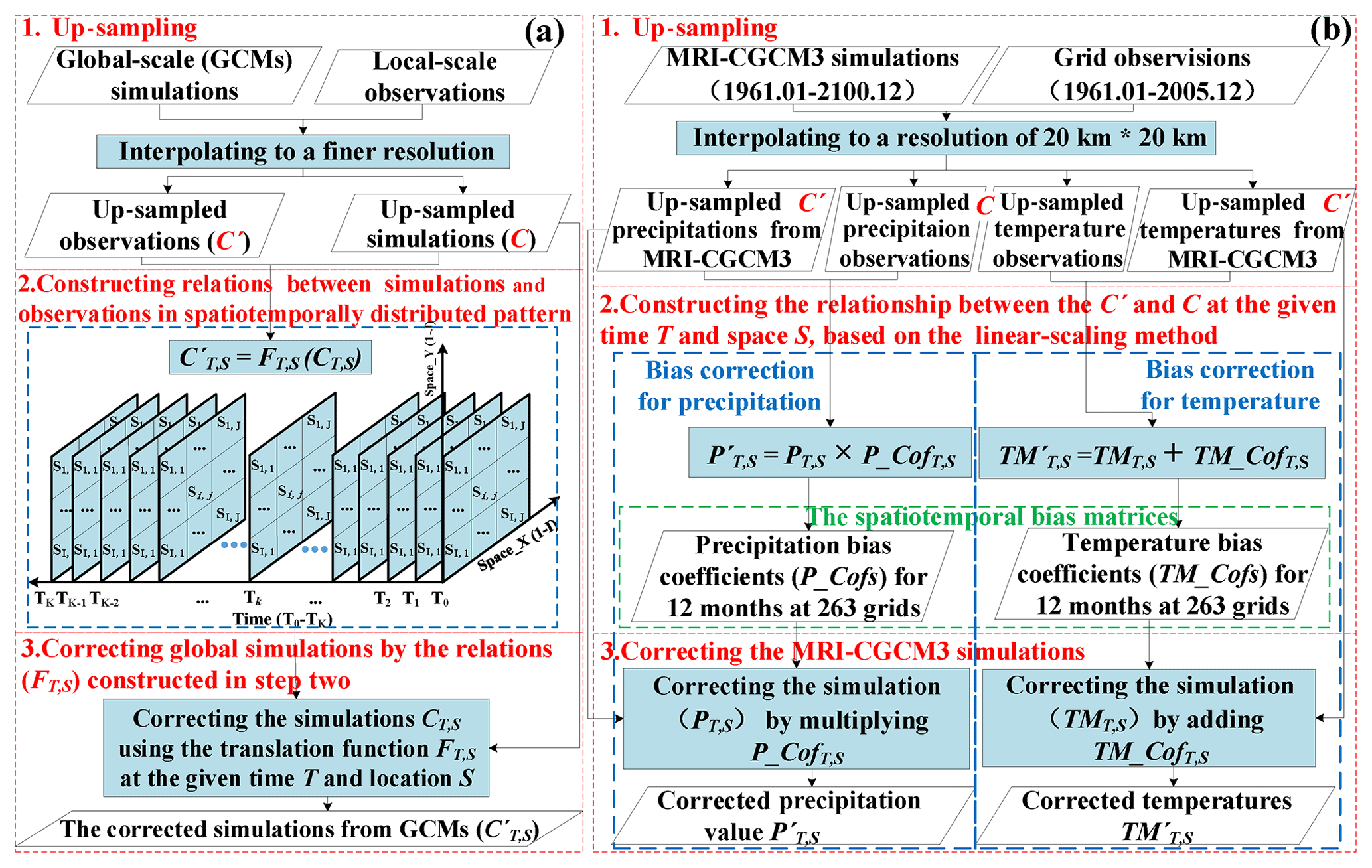
Figure 2Conceptual flow chart of the climate projection including up-sampling, relation construction, and correction; the common framework of the STDDM (a), and the test case based on the linear-scaling algorithm (b). The STDDM was used to project MRI-CGCM3 simulations from 1998 to 2100.
Figure 2a shows the logical framework of the STDDM while Fig. 2b demonstrates how it was applied in the Poyang Lake watershed using MRI-CGCM3 based on a linear-scaling algorithm. The STDDM contains three parts (Fig. 2a, b): (1) up-sampling GCM simulations and local-scale observations to a continuous grid space of the same finer resolution, (2) constructing respective mapping relationship between the GCM simulations and local observations in distributed space and time, and (3) correcting the GCM simulations using the mapping relationship constructed in step two.
3.1.1 Up-sampling GCM simulations
MRI-GCM3 simulations were interpolated by Natural Neighbor Interpolation (Sibson et al., 1981) to a scale of 20 km × 20 km, the smallest size of the sub-basin of the Poyang Lake watershed (Zhang et al., 2017), generating 263 spatial grids (Fig. 2b). For the spatiotemporally distributed downscaling, we used Chinese meteorological spatially continuous grid data as observations, instead of Chinese meteorological station data. We interpolated the gridded observations to 20 km × 20 km, the same as the downscaled climate simulations. The grid pairs of simulations and observations at each time and each grid box were generated.
3.1.2 Constructing relationships between the GCM simulations and local observations
Because there is an inevitable mismatch between the simulations and observations (Li et al., 2010; Wood et al., 2004) after the up-sampling, bias correction should be performed. The bias correction was processed by the transform function between pairs of the up-sampled simulations and observations, which represents the mapping relationship between the pairs. The transform function could be any bias corrected model, including linear scaling, local intensity scaling, power transformation, and the distribution of mapping models (Teutschbein and Seibert, 2012) and other linear or nonlinear regression models.
As the influencing factors on climates show heterogeneity in space and time, we created spatiotemporally distributed relationships, described by the following formula:
where and CT,S indicate the up-sampled global-scale climate simulations and the local climate variables, respectively, in the given time of T and the space of S. FT,S demonstrates a transform function, used to correct the up-sampled GCM simulations. The function is a specific bias correction model, spatiotemporally distributed in mathematic equations or parameters, which is constructed based on the data from the historical period from 1961 to 2005.
In this study, we use a linear-scaling algorithm (Lenderink et al., 2007) as the bias correction model. For the linear-scaling algorithm, the simulations were corrected by the discrepancy between the simulations and observations. Precipitation values derived from the GCMs were corrected by multiplying the precipitation bias coefficient, which is the ratio of the mean monthly observation to simulation from the historical period; temperatures were corrected by adding the temperature bias coefficient, which is the difference between the mean monthly observation and simulation in the historical period. However, as the bias varies among the months from January to December and among the locations of the 236 spatial grids, a global standard bias coefficient is prohibited. To better capture the bias in distributed time and space, we should create an individual bias coefficient for the given month and gird box. Thus, a spatiotemporally distributed bias matrix was constructed. The respective downscaling model and bias coefficient for a given month (T) and space (S) were established by Eqs. (2) and (3):
where P(TM) represents the precipitation (or temperature) of up-sampled simulations, P′ (TM′) represents the downscaled result or up-sampled observations, and PCof (TMCof) represents the bias correction coefficient of precipitation values (or temperatures). In the construction of PCof (TMCof), P (TM) and P′ (TM′) were set as the average monthly precipitation (or temperature) over the historical period, from 1961 to 2005. All the input and output data in the equations are in the given month (T) and space (S).
3.1.3 Correcting the GCM simulations
The constructed relationship between the GCM simulations and the observations from the historical period (in Sect. 3.1.2) also hold for the future (Maraun et al., 2010). Thus, the transform function was used to correct the future CGCM simulations. In this study, we corrected the daily and monthly precipitation values (or temperatures) from MRI-CGCM3 by adding (or multiplying) the bias coefficients in the corresponding month and grid box.
3.2 Precipitation change analysis
3.2.1 Statistic indices of precipitation changes
To obtain the general change in the temporal distribution, we calculated monthly precipitation values from 1998 to 2100, averaged over the whole watershed. As floods and droughts occur more frequently in wet and dry months, we specifically analyze the extreme wet and dry precipitation changes in the 21st century. Therein, monthly precipitation values, >75 % percentile of the 12 months, were classified as the extreme wet monthly precipitation values for each year in the 103-year period; monthly precipitation values, ≤ 25 % percentile were classified as the extreme dry monthly precipitation. The monthly precipitation of the 25 %–50 % and 50 %–75 % quantiles was classified as normal dry and wet monthly precipitation values. The wet monthly precipitation values include extreme and normal wet monthly precipitation values; the dry monthly precipitation values included extreme and normal dry monthly precipitation values. To understand precipitation dynamics in terms of frequency and intensity, daily precipitation values were categorized into five classes based on the classification by the China Meteorological Administration and the possible risk of floods and droughts: light rain, medium rain, heavy rain, rainstorms, and extreme rainstorms, with daily precipitation values of 0.1–10, 10–25, 25–50, 50–100, and >100 mm day−1, respectively. The frequency of precipitation intensities indicates heterogeneity in temporal distribution. The higher the frequency of moderate rain, the more homogeneous the distribution, and the opposite is true for extreme rain. Therefore, the precipitation intensities were separated to moderate or extreme rain. The moderate rain includes light and medium rain, while the extreme rain includes heavy rain, rainstorms, and extreme rainstorms.
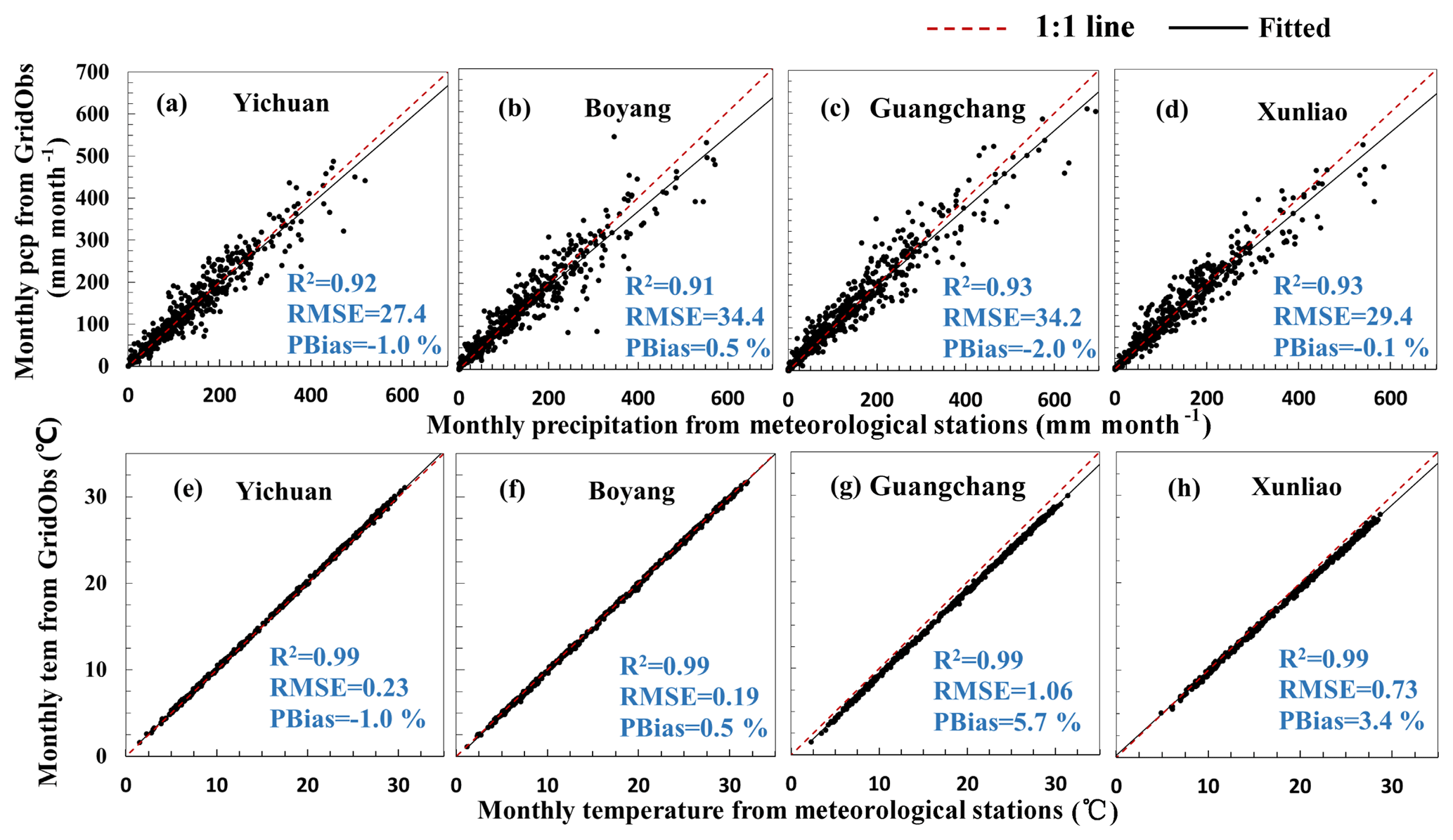
Figure 3Validation of gridded meteorological data (GridObs) by using gauging stations observation: precipitation (pcp; a, b, c, and d) and temperature (tem; e,f,g, and h) at meteorological stations Yichuan (a, e), Boyang (b, f), Guangchang (c, g), and Xunliao (d, f).
To further analyze the changes in precipitation frequencies and intensities, we calculate the annual days of light rain, moderate rain, heavy rain, rainstorms, and extreme rainstorms from 1998 to 2100, averaged over the whole watershed. Annual total precipitation, annual dry days, annual maximum daily precipitation, and annual maximum continuous dry days were displayed as well. The meteorological stations (Fig. 1a) are uniformly distributed in the whole watershed and cover most kinds of the topographies and land covers. Therefore, in the study, all the above precipitation indices for 1 year for the whole watershed were calculated based on the precipitation averaged over the grids containing the 15 stations, instead of using all the grids. Under global climate warming, precipitation becomes more concentrated, which leads to more heterogeneity in temporal and spatial distribution (Donat et al., 2016; Min et al., 2011). Thus, we calculated variation coefficients for each year from 1998 to 2100 to investigate the precipitation changes in temporal and spatial distribution. The variation coefficient measures the standard dispersion of the data items, which can indicate the unevenness of temporal and spatial distributions of the precipitation. In this study, heterogeneity in temporal, spatial, and spatiotemporal distributions was measured by the temporal, spatial and spatiotemporal variation coefficient, respectively. Temporal variation coefficients were calculated from the daily or monthly precipitation values in 1 year, and the variation coefficient for 1 year is averaged from those of the 15 stations. For monthly precipitation, we only select extreme wet and dry precipitation values, as the extreme wet and dry are more likely to cause floods or droughts and thus should be paid more attention to. Spatial variation coefficients were calculated on the annual total precipitation values of the 15 stations in 1 year. The spatiotemporal variation coefficient was calculated on the monthly precipitation values of the extreme wet months of the wet stations and the extreme dry months of the dry stations in 1 year, as the extreme precipitation values were more likely to cause floods or droughts.
3.2.2 Relationship analysis between precipitation changes and increasing temperature
We investigated the precipitation changes as a result of global temperature increase. To this end, we calculated linear regression between the precipitation index and temperature changes from 2005 to 2100. We note that a mean filter with a window size of 21 years can reduce potential random fluctuation from precipitation the most; thus it was used to smooth annual precipitation indices and temperature simulations from 2005 to 2100. The long-term smoothed annual precipitation or temperature minus the average annual value from 1998 to 2017 is set as the precipitation index or temperature changes. A linear regression model was used to investigate whether precipitation changes are related to climate warming. The two 11-year periods, 2005 to 2015 and 2090 to 2100, did not have filter diameter of 21 years at the start and end; thus the climate data used for regression are from 2016 to 2089.
4.1 Model assessment
Validation of the Chinese meteorological grid observations as well as the STDDM should be performed. As the STDDM introduces the Chinese meteorological grid observations, and the grid data are not the direct on-site data, validation of the gridded data is necessary. The determination coefficient (R2), root-mean-square error (RMSE), and PBias (percent bias) were used to examine the model performance.
4.1.1 Evaluation for the gridded meteorological
The Chinese meteorological grid observations are data referenced to corrected GCM simulations, and the reliability of the observations is vital to the performance of the STDDM, so we make a validation using meteorological station observations, as shown in Fig. 3.
As shown in Fig. 3, we select four meteorological stations. The selected stations are uniformly distributed. The validation produced an acceptable precision, with R2>0.91, an absolute PBias<2 % for precipitation values and R2=0.99, and an absolute PBias<6 % for temperature. All the dots of gridded and stationed values were distributed along the 1:1 line, thus confirming the satisfactory performance.
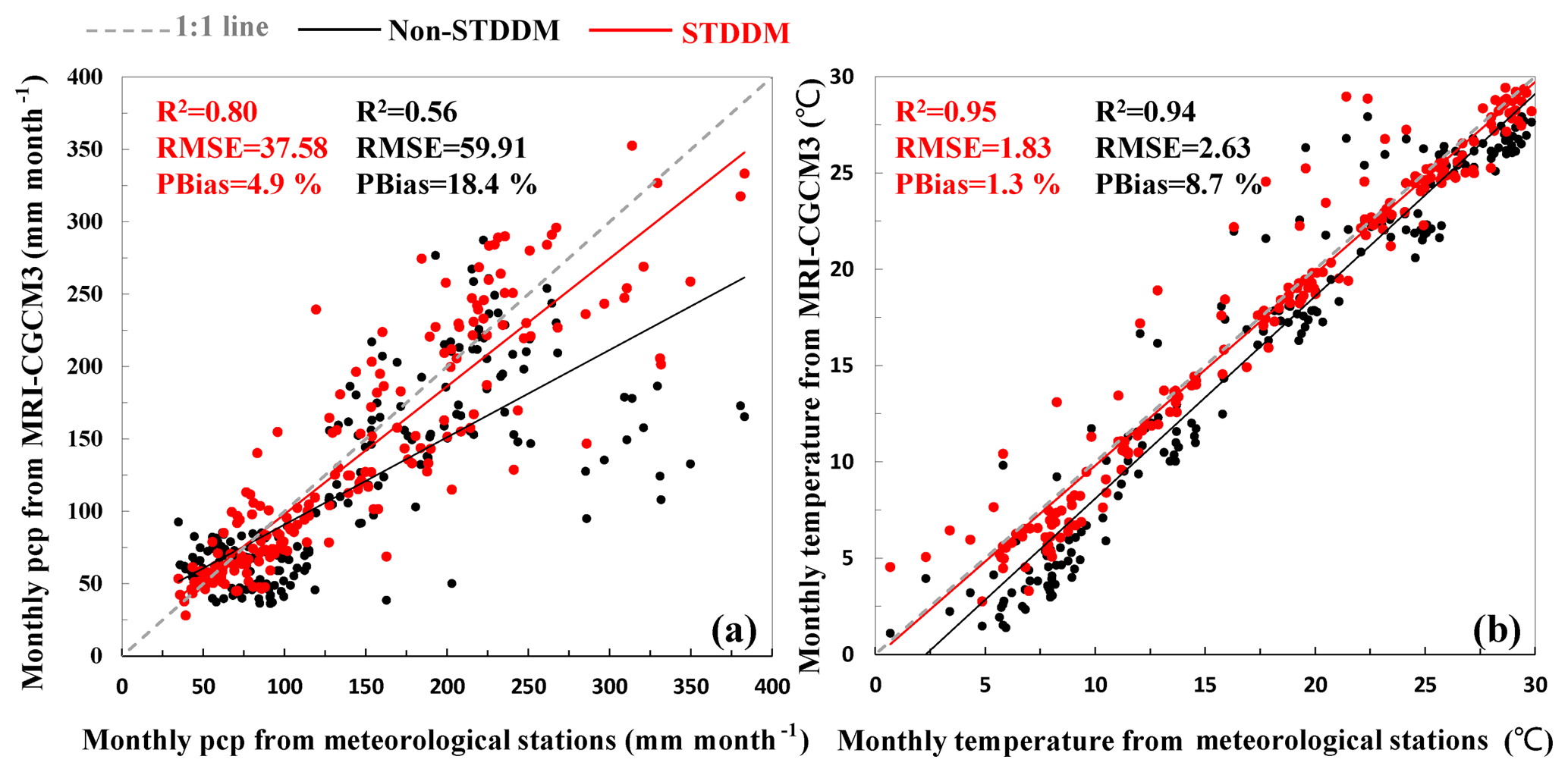
Figure 4Validation of the precipitation (pcp) (a) and temperature (b) projections by the STDDM (in black) and non-STDDM (in red). Dots represent the monthly precipitation values (or temperatures) averaged over 20 years, from 1986 to 2005. The dots contain monthly precipitation values of the 15 stations. The solid lines represent the linear regression that is the best fit of all pairs of the projections and observations.
4.1.2 Validation of precipitation and temperature projections in the Poyang Lake watershed
Before being used in future climate projection, the model should be examined. Data from 1961 to 1985 were used to construct the model, and the remaining historical data from 1986 to 2005 were used to validate it.
To test whether the downscaling method (STDDM) is effective in climate projections, we compare the results before and after the bias correction in Fig. 4. The results before and after the bias correction were marked as the outcomes by the STDDM and non-STDDM, respectively. The projections by the STDDM show better performance, with high correlations and narrow bias, compared to the result of non-STDDM. Considering the complexity of the physical mechanism of the climate and the difficulty of accurately simulating with the present methods, the uncertainty could be acceptable.
Using the STDDM and MRI-CGCMs, we obtained the temporal and spatial variation of future precipitation values in the Poyang Lake watershed and investigated the heterogeneity changes of precipitation in the temporal and spatial distribution.
4.2 Temporal variation of future precipitation
To discover the temporal variation under the future climate warming, we analyzed the monthly and daily precipitation changes during the period from 1998 to 2100. For monthly precipitation, we analyzed intra-annual and inter-annual dynamics of precipitation; based on the dynamics, we investigated the heterogeneity changes of monthly precipitation. For daily precipitation, we analyzed the changes of precipitation intensities and frequencies; based on the changes, heterogeneity changes of daily precipitation were also investigated.

Figure 5Total variability of monthly precipitation from 1998 to 2100. Each column represents the data for 1 year, and each cell represents an accumulative precipitation of 1 month. The red arrows indicate that the monthly precipitation experienced an increasing trend over the 103 years, and the blue arrows indicate that the monthly precipitation experienced a decreasing trend. The asterisk demonstrates the significant trends with p<0.05. (a) Monthly precipitation in the order of the months, referring to spring (March–May), summer (June–August), autumn (September–November), and winter (December to February of the next year), from top to bottom. (b) Monthly precipitation, sorted in the descending order for each year, where months are classified as extreme wet (EWet), normal wet (NWet), normal dry (NDry), and extreme dry (Edry) months, from top to bottom. Therein, wet months (Wet) include extreme and normal wet months, while dry months (Dry) include extreme and normal dry months.
4.2.1 Monthly precipitation changes
We analyzed the monthly precipitation changes during the period from 1998 to 2100, as shown in Fig. 5. Precipitation shows significant intra-annual dynamics. Months with abundant rain (wet months), indicated by a reddish color, are mainly in April–July (the wet season), while the rain-poor months (dry months), indicated by a bluish color, are mainly from September to the subsequent February (the dry season). Precipitation concentrates in spring (March–May) and summer (July–August), occupying 73 % of the annual amount. The intra-annual dynamics of precipitation are similar to those shown by Feng et al. (2012). Precipitation also showed inter-annual dynamics. The wet months become wetter, and the wet season comes earlier from April to March, even in February. In addition, each monthly precipitation value for 7 months (April–November) saw an increasing trend, of which most months (5 months: April, May, June, and August) are in the wet season, while precipitation values of the other 5 months saw a decreasing trend, all of which were in the dry season. It seems that wet months become wetter and dry months become drier, in general.
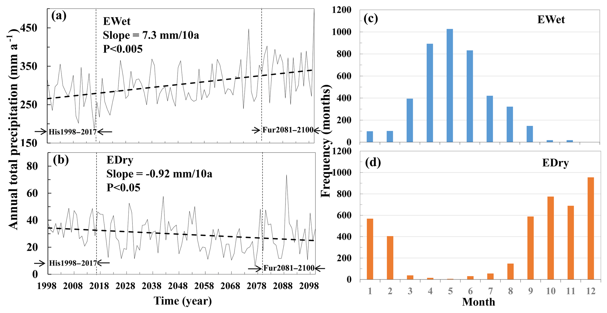
Figure 6The trends of changes in monthly precipitation values of extreme wet (EWet) (a) and dry (EDry) (b) months from 1998 to 2100. The further future period from 2081 to 2100 (Fur2081–2100) and baseline period from 1998 to 2017 (His1998–2017) are indicated by arrows. Frequencies of the months in extreme wet (c) or dry (d) months are calculated during the period from 1998 to 2100.
To better demonstrate the inter-annual dynamics of precipitation, monthly precipitation values in each year were sorted in a descending order in Fig. 5b. Since the time of the monsoon reaching the Poyang Lake watershed varies in different years, with a 1–2 month advance or delay, the wet or dry months for different years are not the same. By sorting monthly precipitation values, wet months and dry months could be distinguished intuitively in Fig. 5b. Obviously, the monthly precipitation values of wet months experienced an increasing trend, and some of these values even had slight significance; in contrast, each dry monthly precipitation value exhibited a decreasing trend, despite being insignificant. We accumulated the extreme wet or dry monthly precipitation values for each year in Fig. 6. The precipitation of extreme wet months showed a significantly increasing trend (p<0.05; Fig. 6a), while the precipitation of the extreme dry months demonstrated a significantly decreasing trend (p<0.05). Extreme wet months increased from 277.82 mm month−1 yr−1 over the historical time period from 1998–2017 to 344.10 mm month−1 yr−1 over the future time period from 2081 to 2100, with a difference of 23.86 % and a rate of change of 7.3 mm month−1 per 10 years. Extreme dry months decreased from 35.44 mm month−1 yr−1 over the historical time period from 1998–2017 to 30.46 mm month−1 yr−1 over the future time period from 2081 to 2100, with a difference of −14.05 % and a rate of change of 0.92 mm month−1 per 10 years. Therein, the extreme wet months are mainly concentrated in March–July (Fig. 6c), part of the wet season, while the extreme dry months are mainly concentrated in September–February (Fig. 6d), consistent with the dry season.
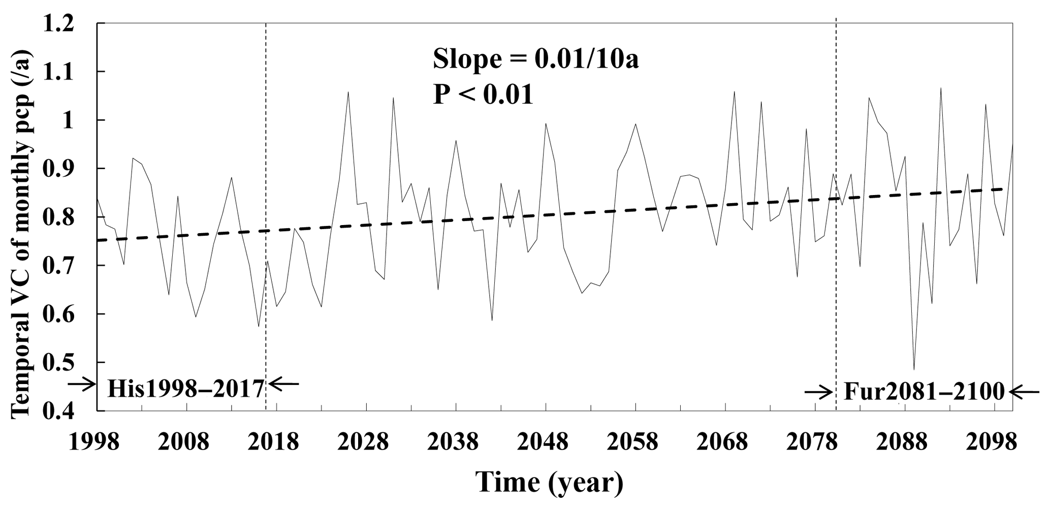
Figure 7The temporal variation coefficient (VCs) of the extreme month precipitation values for each year from 1988 to 2100. The extreme months are composed of the extreme wet and dry months. The far future period from 2081 to 2100 (Fur2081–2100) and baseline period from 1998 to 2017 (His1998–2017) are indicated by arrows.
Overall, under climate warming over the 21st century, the wet month becomes wetter, while the dry month becomes drier, which suggested the uneven temporal distribution of precipitation (Fig. 7). As shown in Fig. 7, the temporal variation coefficient of the extreme month (including extreme wet and months) precipitation values in each year from 1988 to 2100 experience significantly increasing trends (p<0.01) and increased from 0.76 yr−1 over the historical time period from 1998–2017 to 0.84 yr−1 over the future time period from 2081 to 2100, with a difference of 10.53 % and a rate of change of 0.01 per 10 years. The significantly increasing trends indicated the more uneven trend of precipitation in the temporal distribution, which might lead to increased risks of floods and droughts.
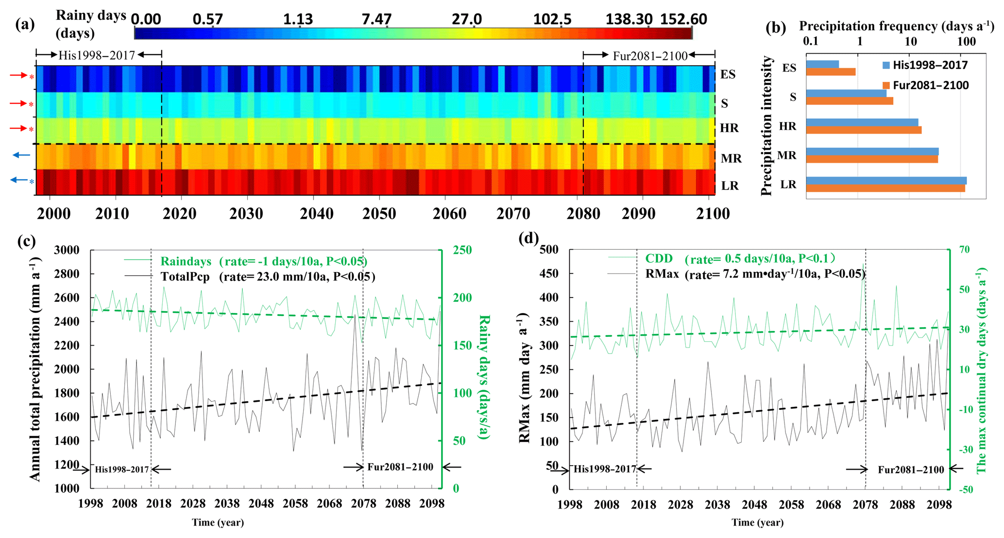
Figure 8The changes in daily precipitation intensities and frequencies. (a) Precipitation intensities and frequencies for each year from 1998 to 2100, where each column represents a year and each row indicates a precipitation intensity. Daily precipitation intensities are categorized into five classes: light rain (LR), moderate rain (MR), heavy rain (HR), rainstorms (S), and extreme rainstorms (ES), with daily precipitation values of 0.1–10, 10–25, 25–50, 50–100, and >100 mm day−1, respectively. The moderate rain includes LR and MR, while the extreme rain is composed of HR, S, and ES. Each cell of (a) represents an annual frequency of one precipitation intensity, with a unit of days. The red arrows indicate that annual frequency of the precipitation intensity experienced an increasing trend over the 103 years (from 1998 to 2100), while the blue arrows indicate a decreasing trend. The asterisk represents the significant trends with p<0.05. The far future period from 2081 to 2100 (Fur2081–2100) and baseline period from 1998 to 2017 (His1998–2017) are indicated by arrows. (b) Precipitation frequencies of LR, MR, HR, S, and ES for Fur2081–2100 and His1998–2017. (c) The change of the long-term data for annual total precipitation (totalPcp) and total rainy days (Raindays). (d) The change in the long-term data for annual maximum daily precipitation (PMax) and annual maximum continuous dry days (CCD).
4.2.2 Daily precipitation changes
To understand the changes in precipitation intensities and frequencies under future climate warming, daily precipitation variations were also analyzed and are shown in Fig. 8. Moderate vs. extreme rain frequencies (Fig. 8a, b), the annual total rain vs. the annual total rainy days (Fig. 8c), and the annual max precipitation vs. the annual maximum continuous rainy days (Fig. 8d) were analyzed.
Under climate warming, the annual frequency of moderate rain experienced decreasing trends; in contrast, the annual frequency of extreme rain experienced significantly increasing trends (Fig. 8a). Statistically, averaged over 103 years, annual precipitation frequencies are dominated by the moderate-rain frequency, on a total of 163.70 or 44.8 % of days (163.70∕365), while the extreme rain occurs less often, on a total of 20.70 or 6.70 % of days (20.7∕365). The remaining are rain-free days, on a total of 180.75 or 49.5 % of days (180.75∕365). The annual moderate-rain frequency decreased, from 170.56 days yr−1 over the historical period from 1998 to 2017 to 159.55 days yr−1 over the future period from 2081 to 2100, with a difference of −6.46 % and a rate of change of −14.4 days per 10 years; on the contrary, the annual extreme rain frequency increased from 19.18 days yr−1 over the historical time period from 1998 to 2017 to 23.42 days yr−1 over the future time period from 2081 to 2100, with a difference of 22.10 % and a rate of change of 0.49 days per 10 years (Fig. 8b).
Furthermore, the annual total rainy days, the sum of the moderate and extreme rain frequencies, demonstrated a significantly decreasing trend in the 21st century, whereas the annual total precipitation exhibited a significantly increasing trend (Fig. 8c). Rainy days decreased from 187.57 days yr−1 over the historical period from 1998 to 2017 to 180.37 days yr−1 over the future period from 2081 to 2100, with a difference of −3.84 % and a rate of change of −1.00 days per 10 years, while the annual total rain amount increased, from 1650 mm yr−1 over the historical period from 1998 to 2017 to 1906 mm yr−1 over the future period from 2081 to 2100, with a difference of 15.55 % and a rate of change of 23.00 mm per 10 years. The increase in the annual total rain and decrease in the annual rainy days suggested more concentrated precipitation and dry days in the future. This tendency might lead to the increased risk of floods and droughts, which was also indicated by the increased annual maximum daily precipitation and maximum continuous dry days (Fig. 8d). Annual maximum daily precipitation increased from 148.76 mm day−1 yr−1, averaged over the historical period from 1998 to 2017, to 212.01 mm day−1 yr−1, averaged over the future period from 2081 to 2100, with a difference of 42.51 % and a rate of change of 7.2 mm day−1 per 10 years, while the maximum continuous dry days increased from 25.35 days yr−1 over the historical period from 1998 to 2017 to 28.15 days yr−1 over the future period from 2081 to 2100, with a difference of 11.05 % and a rate of change of 0.5 days per 10 years.
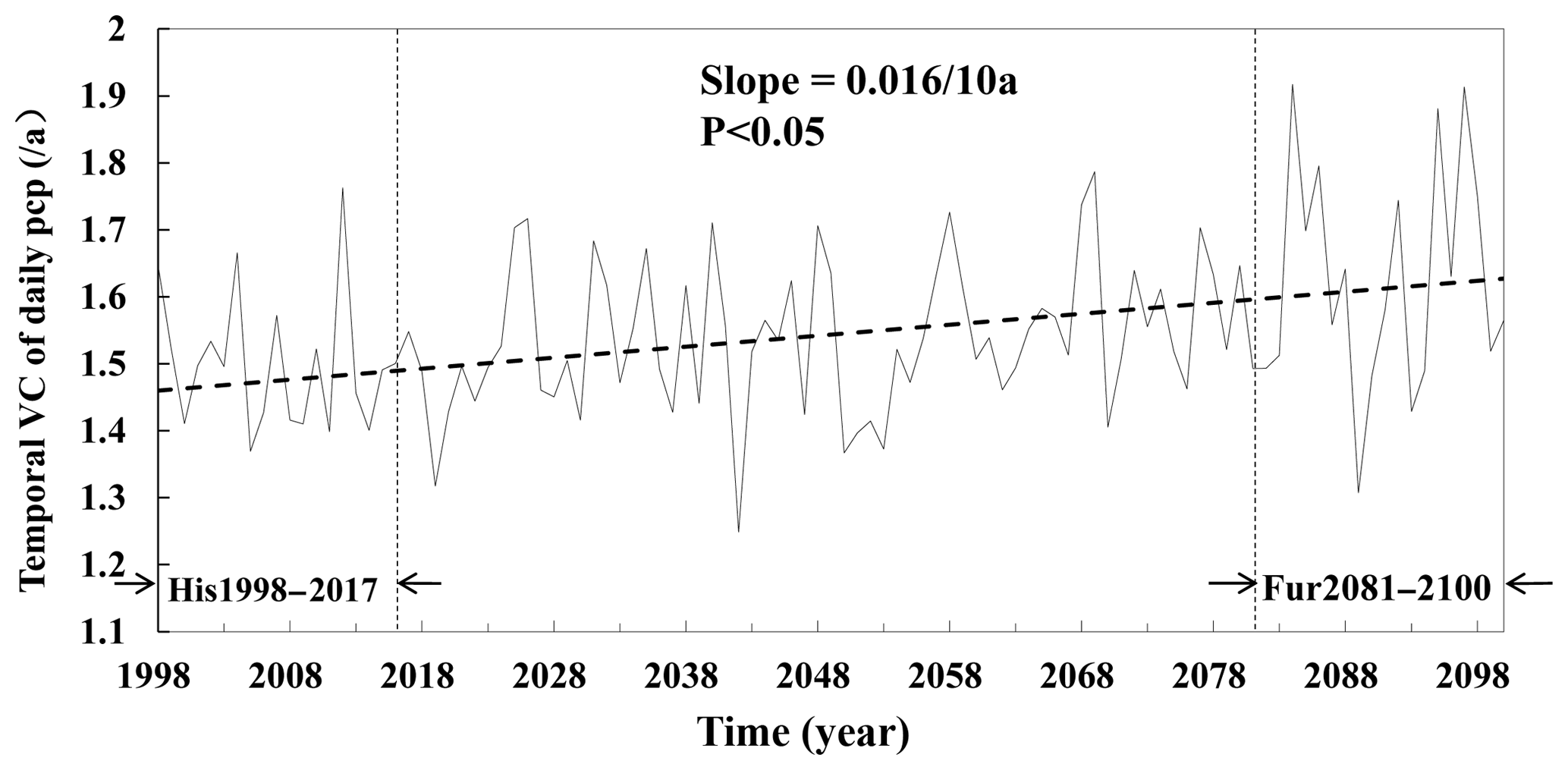
Figure 9The temporal variation coefficient of daily precipitation values for each year from 1988 to 2100. The far future period from 2081 to 2100 (Fur2081–2100) and baseline period from 1998 to 2017 (His1998–2017) are indicated by arrows.
Overall, the significantly inversed trends of change in the moderate vs. extreme rain frequencies, the annual total rain vs. the annual total rainy days, and the annual maximum precipitation vs. the annual maximum continuous rainy days indicated an increasing temporal heterogeneity in precipitation distribution over the 21st century. Obviously, the increasing heterogeneity was exhibited by the increasing temporal variation coefficient of daily precipitation values (Fig. 9). The temporal variation coefficient of daily precipitation values increased from 1.50 yr−1 over the historical period from 1998 to 2017 to 1.62 yr−1 over the future period from 2081 to 2100, with a difference of 7.48 % and a rate of change of 0.016 per 10 years.

Figure 10The precipitation changes in the spatial pattern during the period from 1998 to 2100. Average monthly precipitation values of the wet season (April–July) during the period from 1998 to 2017 (a), 2041 to 2060 (b), and 2081 to 2100 (c), and average monthly precipitation values of the dry season (December to next February) during the historical period from 1998 to 2017 (d), 2041 to 2060 (e), and 2081 to 2100 (f); rate of change of monthly precipitation in wet (g) and dry (h) season from 1998 to 2100. As floods and droughts occur more frequently in extreme months, the precipitation in the analysis considered only the extreme wet (April–July) and dry (September–February) months (Fig. 5c, d). Besides this, precipitation is dominated by the southeastern summer monsoon, which brings water vapor from the sea. The summer monsoon is frequent, from the end of spring to the start of autumn, covering the wet months April–July. However, though they are dry months, the autumn period from September to November is affected by southeastern summer monsoon (Tan, 1994), because, to some extent, autumns are the transpiration periods of summer to winter. Therefore, winter (December–February) was represented as the dry season with poor rain, while April–July was represented as the wet season with abundant rain.
4.3 Spatial variation of future precipitation
Climate warming could cause the rain belt shift (Putnam and Broecker, 2017), which might lead to precipitation changes in the spatial pattern. To investigate the spatial variation, we analyzed the similarities and differences of precipitation changes in space (Fig. 10); based on the differences, we use the indices of the spatial and spatiotemporal variation coefficient to investigate the spatial heterogeneity changes (Fig. 11). Figure 10 shows the precipitation changes in the spatial pattern during the period from 1998 to 2100; Fig. 11 shows the spatial and spatiotemporal variation coefficient for each year from 1988 to 2100.
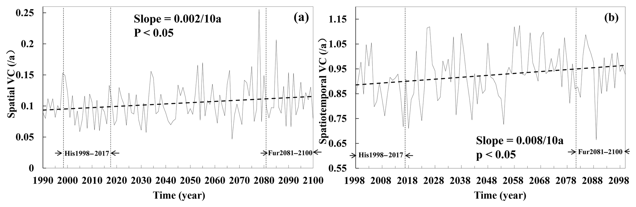
Figure 11The spatial (a) and spatiotemporal (b) variation coefficient for each year from 1988 to 2100. The further future period from 2081 to 2100 (Fur2081–2100) and baseline period from 1998 to 2017 (His1998–2017) are indicated by arrows.
Precipitation values showed a regular spatial pattern in both the wet and dry season, shown in Fig. 10a–c and e–g. More specifically, precipitation was distributed more in the east and west, however it was distributed less in the northern central plain and the southern bottom lowland. Abundant rain in the east and west is dominated by the southeastern and southwestern summer monsoons. Less precipitation was due to the leeward sloop of the eastern (Xuefeng Mountains) and western mountains (Wuyi Mountains). Less precipitation in the southern bottom lowland occurred, because that water vapor was blocked from this region by the Nanling Mountains in the south (Fig. 1a). The precipitation distribution in spatial pattern from 1998 to 2100 (Fig. 10 a–f) was consistent with the observations from 1951 to 2005 (Fig. 1b), thus confirming the satisfactory performance of the STDDM. Moreover, wet and dry season precipitation showed inverse changes. The wet season precipitation values exhibited an increasing (Fig. 10a–c, g) change, while the dry season precipitation exhibited a decreasing (Fig. 10d–h) change from 1998 to 2100. The inverse changes were consistent with the inter-annual variability of increased precipitation in wet months and decreased precipitation in dry months (Sect. 4.2). The increase of precipitation in the wet seasons and decrease in precipitation in the dry seasons were also detected in the rate of change of the cells over the entire watershed (Fig. 10g or h).
However, precipitation change also showed a different spatial pattern. The precipitation rate of change for dry or wet season was heterogeneous in spatial distribution (Fig. 10g, h). In the wet season, the precipitation increased more in the northern part of the watershed, except for the central plain (Fig. 10g); in the dry season, the precipitation decreased more in the central area (Fig. 10h). Statistically, in the wet season, precipitation increased, with the rate of change raising from ≤ 3.6 mm per 10 years in the southwest to ≥ 11.7 mm per 10 years in the northeast; in the dry season, precipitation decreased with the rate of change falling from mm per 10 years in the surrounding region to mm per 10 years in the central region. Furthermore, precipitation changes show different spatial characteristics in wet and dry seasons. From 1998 to 2100, in the wet season (Fig. 10a–c), the wet area (the reddish area, mainly in the north, except for the central plain) becomes wetter; in the dry season (Fig. 10d–f), the dry area (the bluish area, mainly in the northern center plain and in the southern lowland) becomes drier.
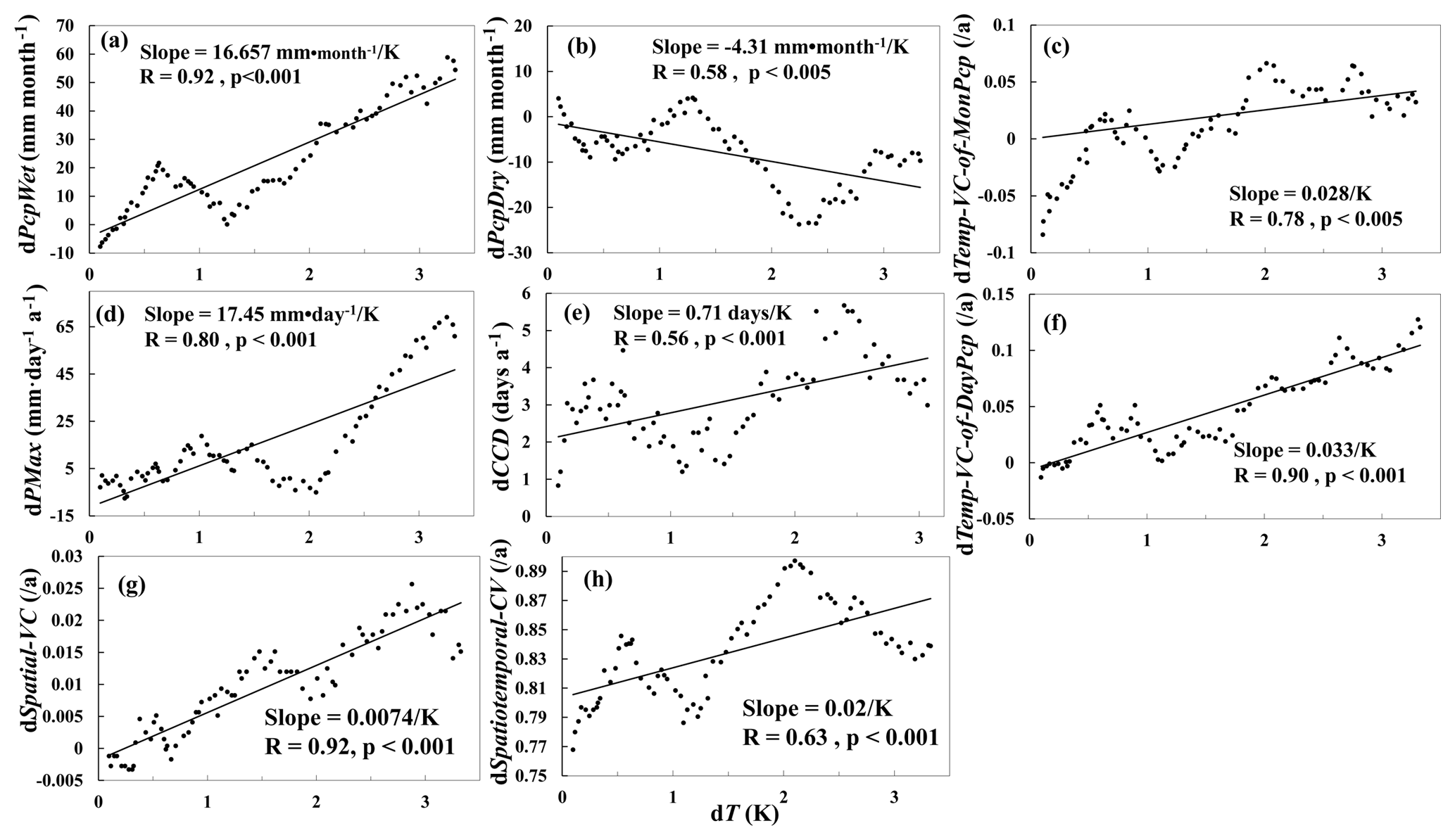
Figure 12The relationship between the precipitation index changes (dPcpIndex) and the temperature increment (dT). The precipitation indices include annual precipitation in the wet season (PcpWet) (a), annual precipitation in the dry season (PcpDry) (b), temporal variance coefficient of monthly precipitation values (Temp-VC-of-MonPcp) (c), annual maximum daily precipitation (PMax) (d), annual maximum continuous dry days (CCD) (e), temporal variance coefficient of daily precipitation values (Temp-VC-of-DayPcp) (f), spatial variance coefficient (Spatial-VC) (g), and spatiotemporal variance coefficient (Spatiotemporal-VC) (h). All the precipitation index changes show significant correlations with temperature increment.
The uneven rates of change may lead to increase of the spatial heterogeneity of precipitation under global warming, and the tendency of the wet area to become wetter and the dry area to become drier also indicated the increasing spatiotemporal heterogeneity of precipitation values. Indeed, the spatial heterogeneity did increase, with the spatial variation coefficients raising from 0.097 yr−1 over the historical period (1998–2017) to 0.110 yr−1 over the future period (2081–2100), with a difference of 12.64 % and a rate of change of 0.002 per 10 years (Fig. 11a). The spatiotemporal heterogeneity did increase with the spatiotemporal variation coefficient raising from 0.89 yr−1 over the historical period (1998–2017) to 0.94 yr−1 over the future period (2081–2100), with a difference of 4.96 % and a rate of change of 0.008 per 10 years. Overall, the uneven rates of change for the whole basin and inverse changes for the dry and wet area indicated increasing spatial heterogeneity in precipitation distribution over the 21st century.
4.4 The impact assessment of temperature increment on precipitation changes
Previous studies have detected precipitation changes and have attributed these changes to climate warming (Westra et al., 2013; Zhang et al., 2013). In this study, the spatiotemporal changes of precipitation in the Poyang Lake watershed in the 21st century were hypothesized to be related to temperature increments. So we analyze the correlations qualitatively and quantitatively.
The following points try to demonstrate the driving force related to climate warming on precipitation changes in the temporal pattern. In the wet season from April to July, the summer monsoon might become weaker in southeastern Asia as the temperature increases (Zhou et al., 2008; Guo et al., 2003). Consequently, the summer monsoon is delayed for a longer time in the middle and lower Yangtze River basin instead of moving further north. The delay leads to much more rain during the wet season. Being located in the middle of the Yangtze River basin, the Poyang Lake watershed becomes wetter in the wet season (Figs. 5, 10a–c). In fact, the increase in precipitation in the Poyang Lake watershed was detected in previous studies (Yu and Zhou, 2007; Ding et al., 2009). In the dry period from September to the subsequent February (especially in the winter season, from December to February), during which summer monsoon is inactive, there is less water vapor in the atmosphere to condense into rain. Additionally, stronger winds in the winter (Wu, Q. et al., 2013) blow the evaporation away, thus enhancing the difficulty of generating rain from water vapor compared to the other seasons. When temperature increases, the ability of the atmosphere to hold water vapor is strengthened, which makes it more difficult to precipitate. Therefore, precipitation decreases in the dry season, consistent with Li et al.'s (2016) results. Since the temperature increment increases the ability of the atmosphere to contain water vapor, rain is more difficult, and if it rains, it will rain heavily (Min et al., 2011; Zhang et al., 2013). Thus, the frequency of heavy rain and rain-free events increases, indicating the increased frequency and strengthened intensity of the extreme precipitation. Overall, climate warming might make precipitation more temporally uneven.
Climate warming could also explain the spatial distribution of precipitation changes in the dry and wet seasons. In the wet season, the summer monsoon is delayed in the middle and lower Yangtze River basin. The delayed area covers only the northern part of the Poyang Lake watershed. As it receives abundant water vapor from the delayed summer monsoon, the northern part of the Poyang Lake watershed experiences a greater increase in precipitation, with a larger rate of change (Fig. 10g). The eastern Poyang Lake watershed is the nearest to the western Pacific Ocean; thus the eastern region receives more continuous water vapor. So the precipitation rate of change decreases from the southeast to the northwest in the wet season. However, in the dry season, especially in winter, during which there is a low-frequency or absent summer monsoon, the water vapor mainly comes from evapotranspiration. In the watershed, the periphery is covered by the Poyang Lake in the northern plain and high-density vegetation in the northwestern, southeastern, and southwestern mountains, so there is more evapotranspiration in the periphery. The center is mainly covered by farmland and grassland, so there is less evapotranspiration in the center (Wu, G. et al., 2013). Thus, the moisture decreases from the surrounding areas to the center. Therefore, as temperature increases, it is more difficult for rain to occur in the area of lower moisture, the center of the Poyang Lake watershed. Therefore the precipitation decreased, with a rate of change falling from the surrounding areas to the center in the dry season (Fig. 10h).
To quantitatively analyze the relationship between precipitation changes and temperature increment, we created scatter plots between precipitation index changes and the temperature increment, as shown in Fig. 12. A trend analysis was conducted using the linear regression of each annual precipitation index over 103 years, from 1998 to 2100. The associated slopes represent the rate of change of each precipitation index, relative to the temperature increment. The significance of the trend is indicated by the p value. As shown in Fig. 12, there is a significant correlation between the precipitation change and the temperature increment, with p≤0.001 and R≥0.78 for six precipitation indices: the annual precipitation in the wet season (Fig. 12a), the annual maximum daily precipitation (Fig. 12d), the temporal variation coefficient of the monthly precipitation (Fig. 12c), the temporal variation coefficient of the daily precipitation (Fig. 12f), the spatial variation coefficient (Fig. 12g), and the spatiotemporal variation coefficient (Fig. 12h). However, changes in the other two precipitation indices, the annual precipitation in the dry season (Fig. 12b) and the annual maximum continuous dry days (Fig. 12e), appeared to be less correlated, with slightly larger values of p≤0.05 and smaller R≤0.58. The overestimation of the moderate-rain frequency from the GCM simulations (Teutschbein and Seibert, 2012; Ines and Hansen, 2006) might explain the slightly low correlation between the annual precipitation values in the dry season and temperature increment, while the overestimation of the precipitation frequencies (Prudhomme et al., 2002) could explain the slightly low correlation between the annual maximum continuous dry days and temperature increment. For all the correlations (Fig. 12a–h), the precipitation changed with fluctuation, which might be caused by random variations from GCMs.
Overall, despite the low correlations and stochastic fluctuation, the correlations could indicate that the climate warming can partly explain the precipitation changes. Statistically, precipitation changes relative to the temperature increment are 16.657 mm month−1 K−1, −4.31 mm month−1 K−1, 17.45 mm day−1 K−1, 0.71 days K−1, 0.028 K−1, 0.033 K−1, 0.0074 K−1, and 0.02 K−1 for the annual precipitation in the wet season, the annual precipitation in the dry season, the annual max daily precipitation, the annual maximum continuous dry days, the temporal variation coefficient of the monthly precipitation, the temporal variation coefficient of the daily precipitation, the spatial variation coefficient, and the spatiotemporal variation coefficient, respectively.
In summary, the explanation of precipitation changes in temporal and spatial distribution, qualitatively and quantitatively, suggests that the downscaling method is reasonable and that the STDDM could be applied successfully to the basin-scale region based on a GCM.
A spatiotemporally distributed downscaling method (STDDM) was proposed in this study. The downscaling method considered the heterogeneity in spatial and temporal distributions and produced local climate variables as spatially continuous data instead of independent and discrete points. The STDDM showed a better performance than the non-STDDM. Using the STDDM, we constructed the spatially continuous future precipitation distribution and dynamics in the wet and dry season from 1998 to 2100, based on the MRI-CGCM3. Several findings were obtained.
First, the spatial and temporal heterogeneity of precipitation increased under future climate warming. In the temporal pattern, the wet season become wetter, while the dry season become drier. The frequency of extreme precipitation increased, while that of the moderate precipitation decreased. Total precipitation increased, while rainy days decreased. Both the maximum dry day number and the maximum daily precipitation increased. These precipitation changes demonstrated an increasing heterogeneity of precipitation in temporal distribution, and the rate of change of temporal heterogeneity is 0.01 per 10 years (0.016 per 10 years) for the temporal variation coefficient of the monthly (daily) precipitation. In the spatial pattern, the rate of change of precipitation was uneven over the whole watershed. Additionally, the wet areas become wetter in the wet season, and the dry areas become drier in the dry season. The uneven rates of change for the whole basin and inverse change for dry and wet areas demonstrated an increasing heterogeneity in the spatial distribution, and the rate of change of spatial heterogeneity was 0.002 per 10 years.
Second, precipitation changes can be significantly explained by climate warming, with p<0.05 and R≥0.56. The explanation of precipitation changes in temporal and spatial distribution, qualitatively and quantitatively, suggests the downscaling method is reasonable and that the STDDM could be successfully applied to the basin-scale region based on a GCM.
The results can be applied to a hydrological and hydrodynamic model to study the future changes in water volumes, lake levels, and regional responses to climate warming. The relationship between precipitation variations and the temperature increment could be helpful for the driving-force analysis of precipitation changes. The condition in which dry becomes drier and wet becomes wetter may lead to an increased risk of floods and droughts. In particular, in the region where floods and droughts do not usually occur, additional adaptation measures could be taken to prevent loss from the future frequent hydrological disasters.
All data can be accessed as described in Sect. 2.2. The data sets and model codes are provided in the Supplement.
The supplement related to this article is available online at: https://doi.org/10.5194/hess-23-1649-2019-supplement.
The project was coordinated by LZ, who took the lead in writing this article. JL and XC outlined the research topic and assisted with the writing of the paper. XF and YZ organized the research collaboration, critically reviewed the paper, and contributed to the writing. DL and QX contributed to the writing and editing of the paper.
The authors declare that they have no conflict of interest.
This work was funded by the National Key Research and Development Program
(2017YFB0504103), the National Natural Science Funding of China (NSFC;
41331174), the Open Foundation of the Jiangxi Engineering Research Center of
Water Engineering Safety and Resources Efficient Utilization (OF201601), the
European Space Agency – Ministry of Science and Technology of China,
Cooperation DRAGON 4 Project (EOWAQYWET), the Fundamental Research Funds for
the Central Universities (2042018kf0220), and the State Key Laboratory of
Information Engineering in Surveying, Mapping and Remote Sensing (LIESMARS)
Special Research Funding.
Edited by: Alexander
Gelfan
Reviewed by: Xianyong Meng and one anonymous referee
Alexander, L. V., Zhang, X., Peterson, T., Caesar, J., Gleason, B., Klein Tank, A. M. G., Haylock, M. R., Collins, W. D., and Trewin, B.: Global observed changes in daily climate extremes of temperature and precipitation, J. Geophys. Res., 111, D05109, https://doi.org/10.1029/2005JD006290, 2006.
Baigorria, G. A. and Jones, J. W.: GiST: A Stochastic Model for Generating Spatially and Temporally Correlated Daily Rainfall Data, J. Climate, 23, 5990–6008, https://doi.org/10.1175/2010jcli3537.1, 2010.
Ben Alaya, M. A., Ouarda, T. B. M. J., and Chebana, F.: Non-Gaussian spatiotemporal simulation of multisite daily precipitation: downscaling framework, Clim. Dynam., 50, 1–15, https://doi.org/10.1007/s00382-017-3578-0, 2018.
Beven, K.: A discussion of distributed hydrological modelling, in: Distributed Hydrological Modelling, edited by: Abbott, M. B. and Refgaard, J. C., Kluwer Academic, the Netherlands, 255–278, 1996.
Boé, J., Terray, L., Habets, F., and Martin, E.: Statistical and dynamical downscaling of the Seine basin climate for hydro-meteorological studies, Int. J. Climatol., 27, 1643–1655, https://doi.org/10.1002/joc.1602, 2007.
Charles, S. P., Bates, B. C., and Hughes, J. P.: A spatiotemporal model for downscaling precipitation occurrence and amounts, J. Geophys. Res.-Atmos., 104, 31657–31669, https://doi.org/10.1029/1999JD900119, 1999.
Chen, H. and Sun, J.: How the “best” models project the future precipitation change in China, Adv. Atmos. Sci., 26, 773–782, https://doi.org/10.1007/s00376-009-8211-7, 2009.
Chen, J., Chen, H., and Guo, S.: Multi-site precipitation downscaling using a stochastic weather generator, Clim. Dynam., 50, 1975–1992, https://doi.org/10.1007/s00382-017-3731-9, 2018.
Chu, J. T., Xia, J., Xu, C. Y., and Singh, V. P.: Statistical downscaling of daily mean temperature, pan evaporation and precipitation for climate change scenarios in Haihe River, China, Theor. Appl. Climatol., 99, 149–161, https://doi.org/10.1007/s00704-009-0129-6, 2010.
Cowpertwait, P. S. P.: A space-time Neyman-Scott model of rainfall: Empirical analysis of extremes, Water Resour. Res., 38, https://doi.org/10.1029/2001WR000709, 2002.
Dai, A.: Increasing drought under global warming in observations and models, Nat. Clim. Chang., 3, 6-1-6-14, https://doi.org/10.1038/nclimate1633, 2013.
DHI (Danish Hydraulic Institute): Mike She, User Manual, Volume 1: User Guide, Hørsholm: Danish Hydraulic Institute, 2014.
Ding, Y., Wang, Z., and Sun, Y.: Inter-decadal variation of the summer precipitation in East China and its association with decreasing Asian summer monsoon, Part I: Observed evidences, Int. J. Climatol., 29, 1926–1944, doi:10.1002/joc.1759, 2009.
Donat, M. G., Lowry, A. L., Alexander, L. V., O'Gorman, P. A., and Maher, N.: More extreme precipitation in the world's dry and wet regions, Nat. Clim. Chang., 6, 508–513, https://doi.org/10.1038/nclimate2941, 2016.
Dyderski, M. K., Paź, S., Frelich, L. E. and Jagodziñski, A. M.: How much does climate change threaten European forest tree species distributions?, Glob. Chang. Biol., 24, 1150–1163, https://doi.org/10.1111/gcb.13925, 2018.
Engman, E. T.: Remote sensing in hydrology, Geophys. Monogr. Ser., 108, 165–177, https://doi.org/10.1029/GM108p0165, 1998.
Enke, W., Schneider, F., and Deutschländer, T.: A novel scheme to derive optimized circulation pattern classifications for downscaling and forecast purposes, Theor. Appl. Climatol., 82, 51–63, https://doi.org/10.1007/s00704-004-0116-x, 2005.
Feng, L., Hu, C., Chen, X., Cai, X., Tian, L., and Gan, W.: Assessment of inundation changes of Poyang Lake using MODIS observations between 2000 and 2010, Remote Sens. Environ., 121, 80–92, https://doi.org/10.1016/j.rse.2012.01.014, 2012.
Fowler, H. J., Blenkinsop, S., and Tebaldi, C.: Linking climate change modelling to impacts studies: Recent advances in downscaling techniques for hydrological modelling, Int. J. Climatol., 27, 1547–1578, https://doi.org/10.1002/joc.1556, 2007.
Frei, C., Schär, C., Lüthi, D., and Davies, H. C.: Heavy precipitation processes in a warmer climate, Geophys. Res. Lett., 25, 1431–1434, https://doi.org/10.1029/98GL51099, 1998.
Giorgi, F.: Simulation of Regional Climate Using a Limited Area Model Nested in a General Circulation Model, J. Climate, 3, 941–963, https://doi.org/10.1175/1520-0442(1990)003<0941:SORCUA>2.0.CO;2, 1990.
Guillot, G. and Lebel, T.: Disaggregation of Sahelian mesoscale convective system rain fields, Further developments and validation, J. Geophys. Res.-Atmos., 104, 31533–31551, https://doi.org/10.1029/1999JD900986, 1999.
Guo, H., Yin, G. Q., and Jiang, T.: Prediction on the possible climate change of Poyang Lake basin in the future 50 years, Resources and Environment in the Yangtze Basin, 17, 73–78, https://doi.org/10.3969/j.issn.1004-8227.2008.01.014, 2008.
Guo, J. L., Guo, S., Guo, J., and Chen, H.: Prediction of Precipitation Change in Poyang Lake Basin, Journal of Yangtze River Scientific Research Institute, 27, 20–24, 2010.
Han, X., Chen, X., and Feng, L.: Four decades of winter wetland changes in Poyang Lake based on Landsat observations between 1973 and 2013, Remote Sens. Environ., 156, 426–437, https://doi.org/10.1016/j.rse.2014.10.003, 2014.
Hong, X., Guo, S., Guo, J., Hou, Y., and Wang, L.: Projected changes of extreme precipitation characteristics in the Poyang Lake Basin based on statistical downscaling model, Water Resour. Res., 3, 511–521, https://doi.org/10.12677/JWRR.2014.36063, 2014.
Hutchinson, M. F.: Interpolation of Rainfall Data with Thin Plate Smoothing Splines – Part I: Two dimensional Smoothing of Data with Short Range Correlation, J. Geogr. Inf. Decis. Anal., 2, 139–151, 1998a.
Hutchinson, M. F.: Interpolation of Rainfall Data with Thin Plate Smoothing Splines – Part II: Analysis of Topographic Dependence, J. Geogr. Inf. Decis. Anal., 2, 152–167, 1998b.Guo H., Yin G. Q., Jiang T.: Prediction on the possible climate change of Poyang Lake basin in the future 50 years, Resources and Environment in the Yangtze Basin, 17(1): 73-78, doi:10.3969/j.issn.1004-8227.2008.01.014 , 2008.
Ines, A. V. M. and Hansen, J. W.: Bias correction of daily GCM rainfall for crop simulation studies, Agricult. Forest Meteorol., 138, 44–53, https://doi.org/10.1016/j.agrformet.2006.03.009, 2006.
Jones, P. D., Wilby, R. L., Wigley, T. M. L., Conway, D., Main, J., Hewitson, B. C., and Wilks, D. S.: Statistical downscaling of general circulation model output: A comparison of methods, Water Resour. Res., 34, 2995–3008, https://doi.org/10.1029/98WR02577, 1998.
Labraga, J. C.: Statistical downscaling estimation of recent rainfall trends in the eastern slope of the Andes mountain range in Argentina, Theor. Appl. Climatol., 99, 287–302, https://doi.org/10.1007/s00704-009-0145-6, 2010.
Leander, R. and Buishand, T. A.: Resampling of regional climate model output for the simulation of extreme river flows, J. Hydrol., 332, 487–496, https://doi.org/10.1016/j.jhydrol.2006.08.006, 2007.
Lenderink, G., Buishand, A., and van Deursen, W.: Estimates of future discharges of the river Rhine using two scenario methodologies: direct versus delta approach, Hydrol. Earth Syst. Sci., 11, 1145–1159, https://doi.org/10.5194/hess-11-1145-2007, 2007.
Li, H., Sheffield, J., and Wood, E.: Bias correction of monthly precipitation and temperature fields from Intergovernmental Panel on Climate Change AR4 models using equidistant quantile, J. Geophys. Res., 115, D10101, https://doi.org/10.1029/2009JD012882, 2010.
Li, Y. L., Tao, H., Yao, J., and Zhang, Q.: Application of a distributed catchment model to investigate hydrological impacts of climate change within Poyang Lake catchment (China), Hydrol. Res., 47, 120–135, https://doi.org/10.2166/nh.2016.234, 2016.
Liang, X., Lettenmaier, D. P., Wood, E. F., and Burges, S. J.: A simple hydrologically based model of land surface water and energy fluxes for general circulation models, J. Geophys. Res.-Atmos., 99, 14415–14428, 1994.
Lovejoy, S. and Schertzer, D.: Multifractals, cloud radiances and rain, J. Hydrol., 322, 59–88, https://doi.org/10.1016/j.jhydrol.2005.02.042, 2006.
Manzanas, R., Lucero, A., Weisheimer, A., and Gutiérrez, J. M.: Can bias correction and statistical downscaling methods improve the skill of seasonal precipitation forecasts?, Clim. Dynam., 50, 1161–1176, https://doi.org/10.1007/s00382-017-3668-z, 2018.
Maurer, E. P. and Hidalgo, H. G.: Utility of daily vs. monthly large-scale climate data: an intercomparison of two statistical downscaling methods, Hydrol. Earth Syst. Sci., 12, 551–563, https://doi.org/10.5194/hess-12-551-2008, 2008.
Maraun, D., Brienn, S., Rust, H. W., Sauter, T., Themeßl, M., Venema, V. K. C., and Chun, K. P.: Precipitation Downscaling Under Climate Change: Recent Developments To Bridge the Gap Between Dynamical Models and the End User, Rev. Geophys., 48, 1–34, https://doi.org/10.1029/2009RG000314, 2010.
Min, S. K., Zhang, X., Zwiers, F. W., and Hegerl, G. C.: Human contribution to more-intense precipitation extremes, Nature, 470, 378–381, https://doi.org/10.1038/nature09763, 2011.
Mullan, D., Chen, J., and Zhang, X. J.: Validation of non-stationary precipitation series for site-specific impact assessment: comparison of two statistical downscaling techniques, Clim. Dynam., 46, 967–986, https://doi.org/10.1007/s00382-015-2626-x, 2016.
Pall, P., Aina, T., Stone, D. A., Stott, P. A., Nozawa, T., Hilberts, A. G. J., Lohmann, D., and Allen, M. R.: Anthropogenic greenhouse gas contribution to flood risk in England and Wales in autumn 2000, Nature, 470, 382–385, https://doi.org/10.1038/nature09762, 2011.
Perica, S. and Foufoula-Georgiou, E.: Model for multiscale disaggregation of spatial rainfall based on coupling meteorological and scaling descriptions, J. Geophys. Res-Atmos., 101, 26347–26361, https://doi.org/10.1029/2009RG000314, 1996.
Prudhomme, C., Reynard, N., and Crooks, S.: Downscaling of global climate models for flood frequency analysis: Where are we now, Hydrol. Proc., 16, 1137–1150, 2002.
Putnam, A. E. and Broecker, W. S.: Human-induced changes in the distribution of rainfall, Sci. Adv., 3, e1600871, https://doi.org/10.1126/sciadv.1600871, 2017.
Quintana Seguí, P., Ribes, A., Martin, E., Habets, F. and Boé, J.: Comparison of three downscaling methods in simulating the impact of climate change on the hydrology of Mediterranean basins, J. Hydrol., 383, 111–124, https://doi.org/10.1016/j.jhydrol.2009.09.050, 2010.
Refsgaard, J. C. and Storm, B., MIKE SHE, in: Computer Models of Watershed Hydrology, edited by: Singh, V. P., Water Resources Publications, Colorado, USA, 809–846, 1995.
Sibson R: A brief description of natural neighbor interpolation, in: Interpreting Multivariate Data, edited by: Barnett, V., Chichester Wiley, 21–36, 1981.
Sperber, K. R., Annamalai, H., Kang, I. S., Kitoh, A., Moise, A., Turner, A., Wang, B., and Zhou, T.: The Asian summer monsoon: An intercomparison of CMIP5 vs. CMIP3 simulations of the late 20th century, Clim. Dynam., 41, 2711–2744, https://doi.org/10.1007/s00382-012-1607-6, 2013.
Tan, R.: A Study on the Regional Energetics during Break, Transitional and Active Periods of the Southwest Monsoon in South East Asia, Scientia Atmospherica Sinica, 18, 527–534, 1994.
Taylor, K. E., Stouffer, R. J., and Meehl, G. A.: An overview of CMIP5 and the experiment desing, B. Am. Meteorol. Soc., 93, 485–498, https://doi.org/10.1175/BAMS-D-11-00094.1, 2012.
Teutschbein, C. and Seibert, J.: Bias correction of regional climate model simulations for hydrological climate-change impact studies: Review and evaluation of different methods, J. Hydrol., 456, 12–29, https://doi.org/10.1016/j.jhydrol.2012.05.052, 2012.
Trenberth, K. E.: Changes in precipitation with climate change, Clim. Res., 47, 123–138, 2011.
Trzaska, S. and Schnarr, E.: A Review of Downscaling Methods for Climate Change Projections, United States Agency for International Development by Tetra Tech ARD: Pasadena, CA, USA, 2014.
Venema, V., Garcíab, S. G., and Simmer, C.: A new algorithm for the downscaling of cloud fields, Q. J. Roy. Meteor. Soc., 136, 91–106, https://doi.org/10.1002/qj.535, 2010.
Von Storch, H. and Zorita, E.: The Analog Method as a Simple Statistical Downscaling Technique: Comparison with More Complicated Methods, J. Climate, 12, 2474–2489, https://doi.org/10.1175/1520-0442(1999)012<2474:TAMAAS>2.0.CO;2, 1999.
Wang, H. Q., Zhao, G. N., Peng, J., and Hu, J. F.: Precipitation characteristics over five major river systems of Poyang drainage areas in recent 50 years, Resources and Environment in the Yangtze Basin, 7, 615–619, 2009.
Wang, J., Hong, Y., Li, L., Gourley, J. J., Khan, S. I., Yilmaz, K. K., Adler, R. F., Policelli, F. S., Habib, S., Irwn, D., Limaye, A. S., Korme, T., and Okello, L.: The coupled routing and excess storage (CREST) distributed hydrological model, Hydrol. Sci. J., 56, 84–98, https://doi.org/10.1080/02626667.2010.543087, 2011.
Westra, S., Alexander, L. V., and Zwiers, F. W.: Global increasing trends in annual maximum daily precipitation, J. Climate, 26, 3904–3918, https://doi.org/10.1175/JCLI-D-12-00502.1, 2013.
Wheater, H. S., Chandler, R. E., Onof, C. J., Isham, V. S., Bellone, E., Yang, C., Lekkas, D., Lourmas, G., and Segond, M. L.: Spatial-temporal rainfall modelling for flood risk estimation, Stoch. Environ. Res. Risk Assess., 19, 403–416, https://doi.org/10.1007/s00477-005-0011-8, 2005.
Wilby, R. L., Dawson, C. W., and Barrow, E. M.: SDSM – a Decision Support Tool for the Assessment of Regional Climate Change Impacts, Environ. Modell. Softw., 17, 145–157, https://doi.org/10.1016/S1364-8152(01)00060-3, 2002.
Wilby, R. L. and Dawson, C. W.: SDSM 4.2-A Decision Support Tool for the Assessment of Regional Climate Change Impacts, Version 4.2, User Manual, Lancaster University, Lancaster/Environment Agency of England and Wales, Lancaster, 1–94, 2007.
Wu, G., Liu, Y., Zhao, X., and Ye, C.: Spatio-temporal variations of evapotranspiration in Poyang Lake Basin using MOD16 products, Geogr. Res., 32, 617–627, 2013.
Wu, Q., Nie, Q., and Zhou, R.: Analysis of wind energy resources reserves and characteristics in mountain area of Jiangxi province, Journal of Natural Resources, 28, 1605–1614, https://doi.org/10.11849/zrzyxb.2013.09.015, 2013.
Wu, J., Zha, J., and Zhao, D.: Evaluating the effects of land use and cover change on the decrease of surface wind speed over China in recent 30 years using a statistical downscaling method, Clim. Dynam., 48, 131–149, https://doi.org/10.1007/s00382-016-3065-z, 2017.
Xu, C. Y.: From GCMs to river flow: A review of downscaling methods and hydrologic modelling approaches, Prog. Phys. Geogr., 23, 229–249, https://doi.org/10.1191/030913399667424608, 1999.
Ye, X., Zhang, Q., Bai, L., and Hu, Q.: A modeling study of catchment discharge to Poyang Lake under future climate in China, Quat. Int., 244, 221–229, https://doi.org/10.1016/j.quaint.2010.07.004, 2011.
Yu, R. and Zhou, T.: Seasonality and three-dimensional structure of interdecadal change in the East Asian monsoon, J. Climate., 20, 5344–5355, https://doi.org/10.1175/2007JCLI1559.1, 2007.
Yuan, W.: Diurnal cycles of precipitation over subtropical China in IPCC AR5 AMIP simulations, Adv. Atmos. Sci., 30, 1679–1694, https://doi.org/10.1007/s00376-013-2250-9, 2013.
Yukimoto, S., Adachi, Y., Hosaka, M., Sakami, T., Yoshimura, H., Hirabara, M., Tanaka, T. Y., Shindo, E., Tsujino, H., Deushi, M., Mizuta, R., Yabu, S., Obata, a, Nakano, H., Koshiro, T., Ose, T., and Kitoh, A.: A New Global Climate Model of the Meteorological Research Institute: MRI-CGCM3-Model Description and Basic Performance, J. Meteorol. Soc. Jpn., 90A, 23–64, https://doi.org/10.2151/jmsj.2012-A02, 2012.
Zhan, M., Yin, J., and Zhang, Y.: Analysis on characteristic of precipitation in Poyang Lake Basin from 1959 to 2008, Procedia Environ. Sci., 10, 1526–1533, https://doi.org/10.1016/j.proenv.2011.09.243, 2011.
Zhang, X. C.: Spatial downscaling of global climate model output for site-specific assessment of crop production and soil erosion, Agr. Forest. Meteorol., 135, 215–229, https://doi.org/10.1016/j.agrformet.2005.11.016, 2005.
Zhang, X., Wan, H., Zwiers, F. W., Hegerl, G. C., and Min, S. K.: Attributing intensification of precipitation extremes to human influence, Geophys. Res. Lett., 40, 5252–5257, https://doi.org/10.1002/grl.51010, 2013.
Zhang, Q., Ye, X. C., Werner, A. D., Li, Y., Liang, Y, J., Li, X. H., and Xu, C. Y.: An investigation of enhanced recessions in Poyang Lake: Comparison of Yangtze River and local catchment impacts, J. Hydrol., 517, 425–434, https://doi.org/10.1016/j.jhydrol.2014.05.051, 2014.
Zhang, L., Lu, J., Chen, X., Liang, D., Fu, X., Sauvage, S., and Sanchez Perez, J.-M.: Stream flow simulation and verification in ungauged zones by coupling hydrological and hydrodynamic models: a case study of the Poyang Lake ungauged zone, Hydrol. Earth Syst. Sci., 21, 5847–5861, https://doi.org/10.5194/hess-21-5847-2017, 2017.
Zhao, Y., Zhu, J., and Xu, Y.: Establishment and assessment of the grid precipitation datasets in China for recent 50 years, J. Meteorol. Sci., 34, 4–10, 2014.
Zhou, T., Yu, R., Li, H., and Wang, B.: Ocean forcing to changes in global monsoon precipitation over the recent half-century, J. Climate, 21, 3833–3852, https://doi.org/10.1175/2008JCLI2067.1, 2008.
Zorita, E. and Von Storch, H.: The analog method as a simple statistical downscaling technique: Comparison with more complicated methods, J. Climate, 12, 2474–2489, https://doi.org/10.1175/1520-0442(1999)012<2474:TAMAAS>2.0.CO;2, 1999.