Multivariate hydrologic design methods under nonstationary conditions and application to engineering practice

Jiang, Cong; Xiong, Lihua; Yan, Lei; Dong, Jianfan; Xu, Chong-Yu

doi:https://doi.org/10.5194/hess-23-1683-2019

Articles | Volume 23, issue 3

https://doi.org/10.5194/hess-23-1683-2019

Articles | Volume 23, issue 3

Research article

22 Mar 2019

Research article |

| 22 Mar 2019

Multivariate hydrologic design methods under nonstationary conditions and application to engineering practice

Cong Jiang, Lihua Xiong, Lei Yan, Jianfan Dong, and Chong-Yu Xu

Abstract

Multivariate hydrologic design under stationary conditions is traditionally performed through the use of the design criterion of the return period, which is theoretically equal to the average inter-arrival time of flood events divided by the exceedance probability of the design flood event. Under nonstationary conditions, the exceedance probability of a given multivariate flood event varies over time. This suggests that the traditional return-period concept cannot apply to engineering practice under nonstationary conditions, since by such a definition, a given multivariate flood event would correspond to a time-varying return period. In this paper, average annual reliability (AAR) was employed as the criterion for multivariate design rather than the return period to ensure that a given multivariate flood event corresponded to a unique design level under nonstationary conditions. The multivariate hydrologic design conditioned on the given AAR was estimated from the nonstationary multivariate flood distribution constructed by a dynamic C-vine copula, allowing for time-varying marginal distributions and a time-varying dependence structure. Both the most-likely design event and confidence interval for the multivariate hydrologic design conditioned on the given AAR were identified to provide supporting information for designers. The multivariate flood series from the Xijiang River, China, were chosen as a case study. The results indicated that both the marginal distributions and dependence structure of the multivariate flood series were nonstationary due to the driving forces of urbanization and reservoir regulation. The nonstationarities of both the marginal distributions and dependence structure were found to affect the outcome of the multivariate hydrologic design.

Download & links

Article (PDF, 8248 KB)

How to cite

How to cite.

Dates

Received: 27 May 2018 – Discussion started: 12 Jul 2018 – Revised: 14 Feb 2019 – Accepted: 09 Mar 2019 – Published: 22 Mar 2019

1 Introduction

A complete flood event or a flood hydrograph contains multiple feature variables, such as flood peak and flood volume, which can be associated with the safety of hydraulic structures (Salvadori et al., 2004, 2007, 2011; Xiao et al., 2009; Xiong et al., 2015; Loveridge et al., 2017; Shafaei et al., 2017). For example, the water level of a reservoir is controlled not only by flood peak flow but also by flood volume (Salvadori et al., 2011). Therefore, multivariate hydrologic design, which takes into account multiple flood characteristics as well as their dependence, provides a more rational design strategy for hydraulic structures compared to univariate hydrologic design (Zheng et al., 2013, 2014; Balistrocchi and Bacchi, 2017).

Multivariate hydrologic design under stationary conditions has been widely investigated, and the design criterion is usually quantified by the return period, similar to univariate hydrologic design. Under the definition of the average recurrence interval between flood events equaling or exceeding a given threshold (Chow, 1964), the return period of a given flood event under stationary conditions theoretically equals the average inter-arrival time between flood events divided by the exceedance probability (Salvadori et al., 2011). On the other hand, the exceedance probability of a univariate flood event is usually uniquely defined without ambiguity, whereas the exceedance probability of a multivariate flood event could have multiple definitions (Salvadori and De Michele, 2004; Salvadori et al., 2011; Vandenberghe et al., 2011). To date, at least five kinds of different exceedance probabilities for a multivariate flood event have been defined: (1) the OR case in which at least one of the flood features exceeds the prescribed threshold, (2) the AND case in which all flood features exceed the prescribed thresholds, (3) the Kendall case in which the univariate representation transformed from Kendall's distribution function exceeds the prescribed threshold, (4) the survival Kendall case in which the univariate representation transformed from survival Kendall's distribution function exceeds the prescribed threshold, and (5) the structural case in which the univariate representation transformed from a structure function exceeds the prescribed threshold (Favre et al., 2004; Salvadori and De Michele, 2004, 2010; Salvadori et al., 2007, 2013, 2015, 2016; Vandenberghe et al., 2011; Requena et al., 2013; Zheng et al., 2014).

Due to climate change as well as certain anthropogenic driving forces (Milly et al., 2008), the nonstationarities of both univariate and multivariate flood series have been widely reported (Xiong and Guo, 2004; Villarini et al., 2009; Vogel et al., 2011; López and Francés, 2013; Bender et al., 2014; Xiong et al., 2015; Blöschl et al., 2017; Kundzewicz et al., 2018). The multivariate flood distribution exhibits more complex nonstationarity behaviours than the univariate distribution, including nonstationarities of individual margins and the dependence structure between the margins (Quessy et al., 2013; Bender et al., 2014; Xiong et al., 2015; Kwon et al., 2016; Sarhadi et al., 2016; Qi and Liu, 2017; Vezzoli et al., 2017; Bracken et al., 2018; Salvadori et al., 2018). Both nonstationarities of the margins and dependence structure could impact the multivariate hydrologic design. Under nonstationary conditions, the exceedance probability p of a given flood event varies from year to year; thus, the return period, calculated as the average inter-arrival time between two successive flood events divided by p, is no longer a constant (Salas and Obeysekera, 2014; Jiang et al., 2015a; Kwon et al., 2016; Sarhadi et al., 2016; Yan et al., 2017). As a result, a given flood event would correspond to a time-varying and non-unique return period. Consequently, the traditional return-period-based method for estimating hydrologic design may no longer be applicable to engineering practice under nonstationary conditions (Salas and Obeysekera, 2014).

Although increasing attention has been focused on the hydrologic designs under nonstationary conditions in recent years, the focus has mainly been on univariate designs (Obeysekera and Salas, 2014, 2016; Read and Vogel, 2016). To overcome the limitation of the traditional return period under nonstationary conditions, the concept of the return period has been revisited. Salas and Obeysekera (2014) extended two concepts of the return period into a nonstationary framework, defined as the expected waiting time (EWT) for an exceedance to occur (Olsen et al., 1998), and the time period that results in the expected number of exceedances (ENE) equal to 1 over this period (Parey et al., 2010).

Risk and reliability are both important measurements for assessing hydrologic designs (Vogel, 1987; Read and Vogel, 2015). Besides redefinitions of the return period, some risk-based or reliability-based metrics have been introduced as the hydrologic design criteria under nonstationary conditions (Rosner et al., 2014). Rootzén and Katz (2013) proposed the concept of the design life level (DLL) to quantify hydrologic risk in a nonstationary climate during the entire design life period of hydraulic structures. Read and Vogel (2015) introduced the concept of average annual reliability (AAR) to estimate the hydrologic designs under nonstationary conditions. Liang et al. (2016) defined the equivalent reliability (ER) to estimate the design flood under nonstationary conditions by linking the DLL to the return period. Salvadori et al. (2018) associated hydrologic designs with both given life times and failure probabilities to calculate bivariate design values under nonstationarity. These design criteria assess the risk or reliability of hydraulic structures associated with the flood distribution during the entire design life period, rather than for a single year. For a given design life period, these criteria can always yield a unique risk or reliability; therefore, they are applicable to the hydrologic designs under both stationary and nonstationary conditions.

Under the multivariate framework, a given design level would correspond to an infinite number of possible hydrologic design events (Hawkes, 2008; Kew et al., 2013; Zheng et al., 2015, 2017); however, these design events are generally not equivalent because their joint probability density values (i.e. likelihood) usually differ (Salvadori et al., 2011; Volpi and Fiori, 2012; Li et al., 2017; Yin et al., 2017). In engineering practice, it should be necessary to determine a typical design event as representative of a specific design level. For example, in Chinese engineering practice, a unique design flood hydrograph corresponding to a given design level is usually required to determine the scale of hydraulic structures (Yin et al., 2017). The most-likely design event, which theoretically has the largest joint probability density (likelihood) among all possible design events (Salvadori et al., 2011), appears to be the best representative candidate. Besides the most-likely design event, it is also necessary to identify the confidence interval for an infinite possible number of design events to provide a finite design range for designers (Volpi and Fiori, 2012; Yin et al., 2017). The most-likely design event and confidence interval for the bivariate hydrologic design under stationary conditions have been identified (Salvadori et al., 2011; Volpi and Fiori, 2012; Li et al., 2017; Yin et al., 2017; Salvadori et al., 2018); however, very few studies have focused on hydrologic designs with higher dimensions under nonstationary conditions.

Therefore, the objective of the present study was to address the issue of multivariate hydrologic design applying to engineering practice under nonstationary conditions, which is achieved through the following steps. First, the nonstationary multivariate flood distribution was constructed using a dynamic canonical vine (C-vine) copula (Aas et al., 2009), which was able to capture the nonstationarities of both marginal distributions and the dependence structure. The design criterion for the multivariate flood event was then quantified according to AAR rather than the traditional return period, since a given multivariate flood event would correspond to a unique AAR under both stationary and nonstationary conditions (Read and Vogel, 2015; Yan et al., 2017). The multivariate hydrologic design for any given AAR was estimated from the nonstationary multivariate flood distribution.

The aforementioned methods for the multivariate hydrologic design under nonstationary conditions were applied to the Xijiang River, China. The four-dimensional (4-D) multivariate flood series, including the annual maximum daily discharge, annual maximum 3-day flood volume, annual maximum 7-day flood volume and annual maximum 15-day flood volume of the Xijiang River were chosen as the case study data because they constitute the variables used for deriving the design flood hydrograph for hydraulic structures. It has been found that the natural flood processes of this river have been significantly altered by urbanization and reservoir regulation (Xu et al., 2014), but these two factors have not yet been taken into account in multivariate hydrologic design.

The next section of the present paper describes the study area and data. Section 3 presents the methods developed in this paper. The results of the case study are provided in Sect. 4. Finally, the conclusion and remarks are provided in Sect. 5.

2 Study area and data

The multivariate flood series of the Xijiang River, South China (see Fig. 1), were selected as a case study to illustrate the multivariate hydrologic design methods under nonstationary conditions. The drainage area of the Xijiang River basin (XRB) is 353 120 km², with a river length of 2214 km. The basin falls within a humid subtropical monsoon climate region, with the flood season extending from May to October; therefore, floods have always been a serious natural hazard within the basin.

https://www.hydrol-earth-syst-sci.net/23/1683/2019/hess-23-1683-2019-f01

Figure 1Map of the Xijiang River basin (above the Dahuangjiangkou gauge).

Download

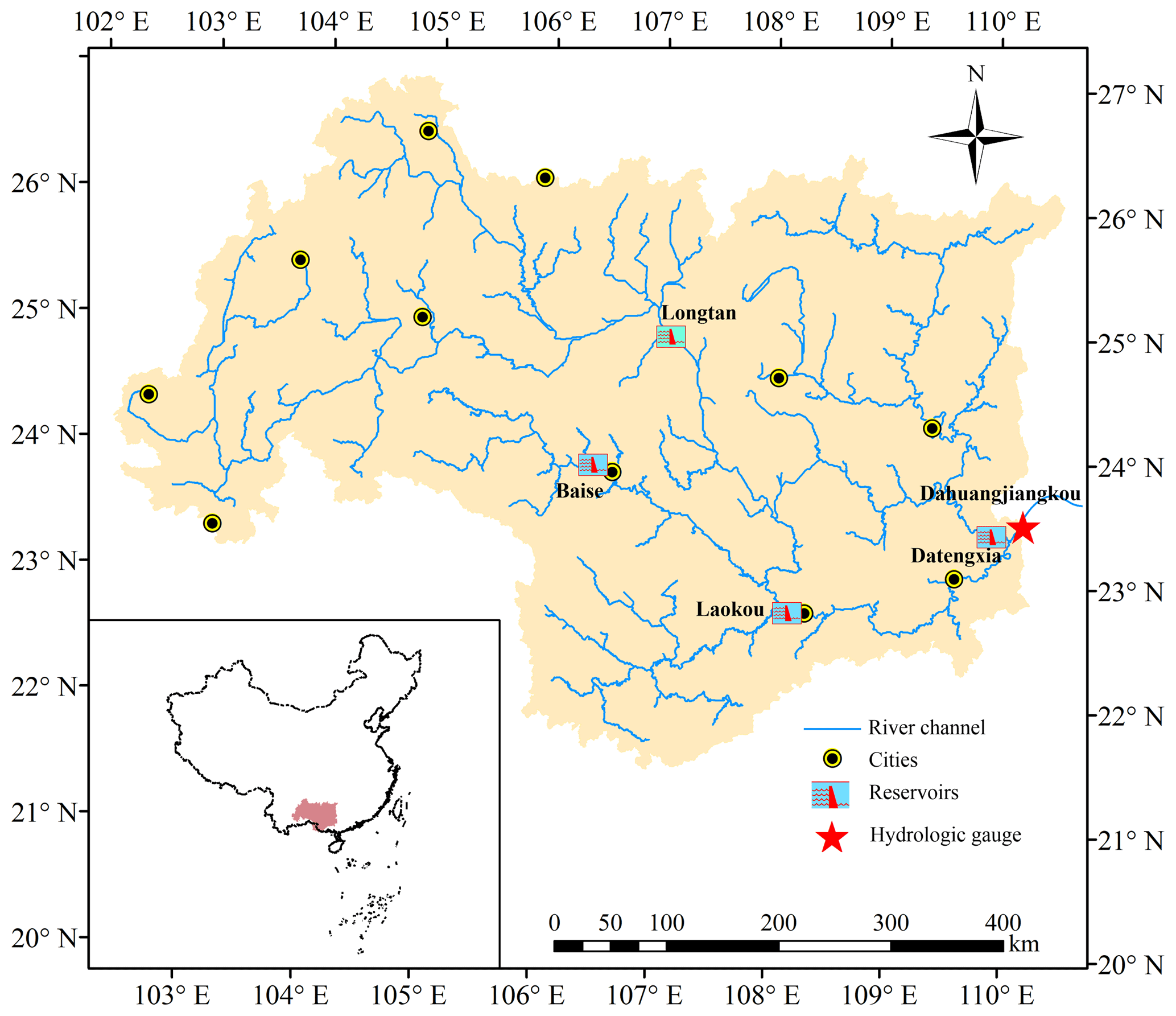
The calculation of design floods in China involving the derivation of flood hydrographs for hydraulic structures requires not only flood peak but also flood volumes with different durations, such as 3, 7, 15 and 30 days (Ministry of Water Resources of People's Republic of China, 1996; Xiao et al., 2009; Xiong et al., 2015; Li et al., 2017). For a large catchment such as the XRB, the duration of a flood process is usually longer than 10 days. Therefore, the annual maximum daily discharge (Q₁), annual maximum 3-day flood volume (V₃), annual maximum 7-day flood volume (V₇) and annual maximum 15-day flood volume (V₁₅) of the Xijiang River were defined as the multivariate flood series $(Q_{1}, V_{3}, V_{7}, V_{15})$ for deriving design flood hydrographs. The flood data were from 1951 to 2012 and observed at the Dahuangjiangkou gauge located at the main stream of the Xijiang River, draining a total catchment area of 294 669 km², approximately 83 % of the total area of the XRB.

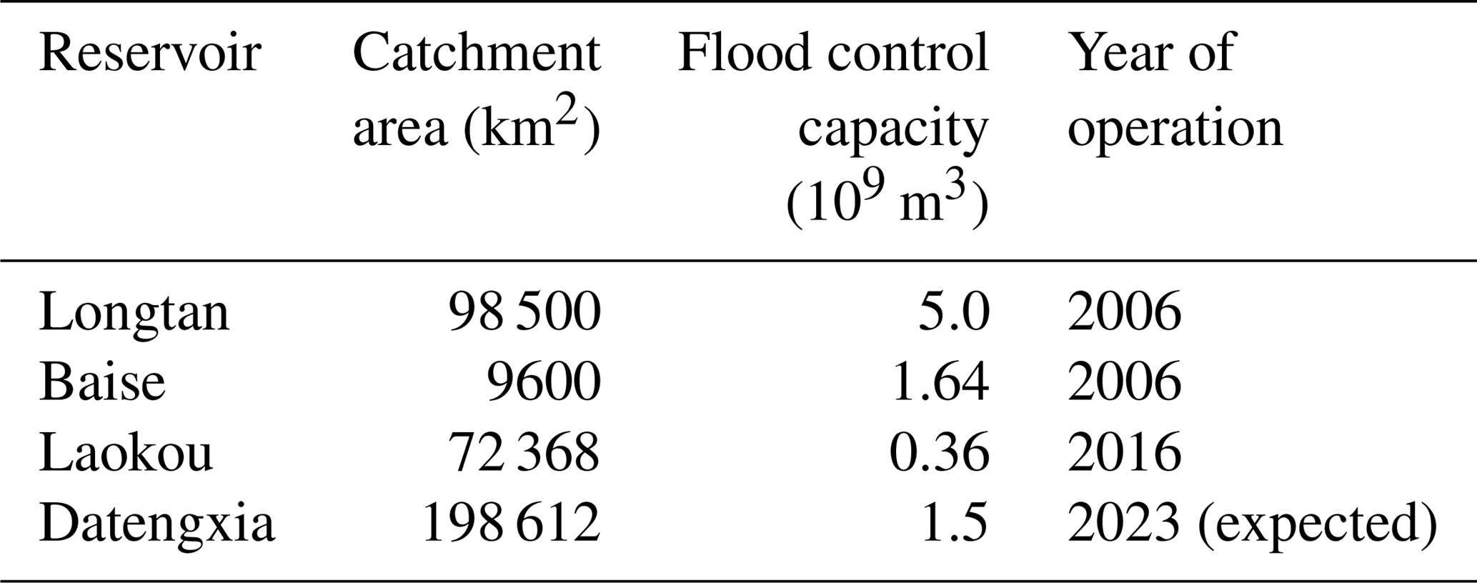
Rapid urbanization over recent decades has resulted in increasing river regulation projects built in the XRB, such as artificial levees for protecting urban areas from river flooding. As a result, flood flow has become increasingly constrained to the channel rather than overflowing to the floodplain, resulting in an increase in the observed river flood flow (Xu et al., 2014). For the purpose of flood control and hydropower generation, it is hard to find a river which is not impacted by reservoirs, particularly in rapidly developing China. Reservoir regulation has become an increasingly significant factor affecting flood processes of the XRB and should be seriously considered within downstream flood risk analysis and hydrologic design, particularly after 2006, when two reservoirs with considerable flood control capacities were put into operation. These are the Longtan and Baise reservoirs, with flood control capacities of 5 × 10⁹ m³ and 1.64×10⁹ m³ and catchment areas of 98 500 and 9600 km², respectively. Climate change will likely result in flood nonstationarity by altering climatic conditions of the basin. Climatic conditions dominating flood processes in the XRB, such as extreme precipitation, appear to have been stationary over the past decades (Yang et al., 2010). Therefore, the current study introduced only urbanization and reservoir regulation as the potential driving forces of flood nonstationarity and ignored the effect of climate change.

The effect of urbanization on flood processes was quantified using the urban population (Pop). Given the unavailability of urban population data at the basin scale and the fact that the vast majority of cities in the XRB are distributed in Guangxi province, we used urban population data for Guangxi province to represent those of the XRB. The annual urban population data during the observation period were obtained from the China Compendium of Statistics 1949–2008 (Department of Comprehensive Statistics of National Bureau of Statistics, 2010) and the website of the National Bureau of Statistics of China (http://www.stats.gov.cn/tjsj/ndsj/, last access: 20 March 2019). The present study assumed the design life period for hydraulic structures to be from 2013 to 2100. The urban population over the design life period was estimated based on the predicted growth rate of China's urban population reported by He (2014). The reservoir index (RI), which depends on the catchment area and flood controlling capacities of reservoirs, was used to quantify the effects of reservoir regulation on flood processes (López and Francés, 2013). As shown in Table 1, two reservoirs with flood control functions have been completed during the observation period from 1951 to 2012, and a further two are planned for operation during the design life period. Figure 2 illustrates the evolution of the urban population and reservoir index during both the observation and design life periods.

https://www.hydrol-earth-syst-sci.net/23/1683/2019/hess-23-1683-2019-f02

Figure 2Evolution of the urban population and reservoir index during both the observation and design life periods.

Download

Table 1Reservoir information for the Xijiang River basin.

Download Print Version | Download XLSX

3 Methods

The present study included the following methods: (1) the nonstationary multivariate flood distribution based on a dynamic C-vine copula, allowing for both time-varying marginal distributions and a time-varying dependence structure, and (2) estimation of the multivariate hydrologic design associated with AAR under nonstationary conditions. To correspond to the case study in this paper, the multivariate flood series consisting of the annual maximum daily discharge (Q₁), annual maximum 3-day flood volume (V₃), annual maximum 7-day flood volume (V₇) and annual maximum 15-day flood volume (V₁₅) were chosen to illustrate the multivariate design methods under nonstationary conditions. It is worth noting that the proposed methods can be extended to other multivariate flood series, such as those consisting of flood peak, flood volume and flood duration.

3.1 Probability distribution of the nonstationary multivariate flood series

According to Sklar's theorem (Sklar, 1959), the probability distribution of the 4-D flood series $(Q_{1}, V_{3}, V_{7}, V_{15})$ at time t measured by years ( $t = 1, 2, \dots, n$ , and n is the length of the flood series) can be formulated through a copula C(⋅) as follows:

\begin{array}{l} F (q_{1, t}, v_{3, t}, v_{7, t}, v_{15, t} |θ_{t}) \\ = C [F_{1} (q_{1, t} | θ_{1, t}), F_{3} (v_{3, t} | θ_{3, t}), F_{7} (v_{7, t} | θ_{7, t}), \\ F_{15} (v_{15, t} | θ_{15, t}) | θ_{c, t}] \\ (1) & = C (u_{1, t}, u_{3, t}, u_{7, t}, u_{15, t} | θ_{c, t}), \end{array}

where $F_{1} (q_{1, t} | θ_{1, t})$ , $F_{3} (v_{3, t} | θ_{3, t})$ , $F_{7} (v_{7, t} | θ_{7, t})$ and $F_{15} (v_{15, t} | θ_{15, t})$ denote the marginal distributions for Q₁, V₃, V₇ and V₁₅, respectively; u_1, t, u_3, t, u_7, t and u_15, t are the marginal probabilities of Q₁, V₃, V₇ and V₁₅, respectively; θ_1, t, θ_3, t, θ_7, t and θ_15, t are the corresponding distribution parameters; and θ_c, t stands for the copula parameter vector, which describes the strength of the dependence structure. $θ_{t} = (θ_{1, t}, θ_{3, t}, θ_{7, t}, θ_{15, t}, θ_{c, t})$ is the parameter vector of the entire multivariate distribution, including the marginal distribution parameters as well as the copula parameters.

According to the multivariate distribution of $(Q_{1}, V_{3}, V_{7}, V_{15})$ defined by Eq. (1), the corresponding density function can be written as:

\begin{array}{l} f (q_{1, t}, v_{3, t}, v_{7, t}, v_{15, t} |θ_{t}) \\ = c [F_{1} (q_{1, t} | θ_{1, t}), F_{3} (v_{3, t} | θ_{3, t}), F_{7} (v_{7, t} | θ_{7, t}), \\ F_{15} (v_{15, t} | θ_{15, t}) | θ_{c, t}] \cdot f_{1} (q_{1, t} | θ_{1, t}) \cdot f_{3} (v_{3, t} | θ_{3, t}) \\ \cdot f_{7} (v_{7, t} | θ_{7, t}) \cdot f_{15} (v_{15, t} | θ_{15, t}) \\ = c (u_{1, t}, u_{3, t}, u_{7, t}, u_{15, t} | θ_{c, t}) \cdot f_{1} (q_{1, t} | θ_{1, t}) \\ (2) & \cdot f_{3} (v_{3, t} | θ_{3, t}) \cdot f_{7} (v_{7, t} | θ_{7, t}) \cdot f_{15} (v_{15, t} | θ_{15, t}), \end{array}

where $f_{1} (q_{1, t} | θ_{1, t})$ , $f_{3} (v_{3, t} | θ_{3, t})$ , $f_{7} (v_{7, t} | θ_{7, t})$ and $f_{15} (v_{15, t} | θ_{15, t})$ are the density functions of the marginal distributions for Q₁, V₃, V₇ and V₁₅, respectively, and c(⋅) denotes the density function of copula C(⋅). As shown by Eq. (2), the multivariate distribution of $(Q_{1}, V_{3}, V_{7}, V_{15})$ can be separated into two modules, including the marginal distributions, i.e. $f_{1} (q_{1, t} | θ_{1, t})$ , $f_{3} (v_{3, t} | θ_{3, t})$ , $f_{7} (v_{7, t} | θ_{7, t})$ and $f_{15} (v_{15, t} | θ_{15, t})$ , as well as the dependence structure expressed by the copula density function $c (u_{1, t}, u_{3, t}, u_{7, t}, u_{15, t} | θ_{c, t})$ . Under nonstationary conditions, both the margins and dependence structure of $(Q_{1}, V_{3}, V_{7}, V_{15})$ can vary over time t.

3.1.1 Nonstationary marginal distributions based on the time-varying moment model

The time-varying moment model that expresses the distribution parameters or moments as functions of time or some other explanatory variable or variables have been widely employed to capture the nonstationarities of univariate flood series (Strupczewski et al., 2001; Villarini et al., 2009). In this study, the nonstationary marginal distributions of the multivariate flood series $(Q_{1}, V_{3}, V_{7}, V_{15})$ were constructed by the time-varying moment model.

Based on cause–effect analysis, the flood processes of the XRB were found to mainly be impacted by urbanization and reservoir operation. The reservoir index RI and urban population Pop were therefore used as potential covariates for marginal distribution parameters, including the location parameter μ, scale parameter σ and shape parameter ν (if any). In this study, both linear and exponential functions were considered to build the relationships between distribution parameters and covariates (Strupczewski et al., 2001; Vogel et al., 2011; Salas and Obeysekera, 2014; Jiang et al., 2015; Sarhadi et al., 2016; Read and Vogel, 2016; Yan et al., 2017). Taking the location parameter for illustration, the candidate functions of μ were generally formulated as follows.

\begin{matrix} (3) & \begin{array}{ll} Linear : & μ_{t} = α_{0} + α_{1} {Pop}_{t} + α_{2} {RI}_{t} . \\ Exponential : & μ_{t} = \exp (α_{0} + α_{1} {Pop}_{t} + α_{2} {RI}_{t}) . \end{array} \end{matrix}

Here α₀, α₁ and α₂ are model parameters estimated using the maximum likelihood estimate (MLE) method (Strupczewski et al., 2001). As above, the linear expression in Eq. (3) gives an additive model which suggests that the effects of the covariates RI and Pop on μ are independent, while the exponential expression defines a multiplicative model which is able to take into account the possible interaction between the covariates RI and Pop. It is important to note that Eq. (3) defines four specific nonstationary models: the first one is the most complex nonstationary model where it is assumed that both RI and Pop are the driving factors of marginal distributions, the second and third models illustrate that the marginal nonstationarity is linked only to RI and Pop, respectively, and the final one represents the simplest and stationary model, which does not contain any covariates.

Five probability distributions widely used in flood frequency analysis, namely Pearson type III (PIII), generalized extreme value (GEV), gamma, Weibull and lognormal distributions, were employed as the candidate distributions for margins (Villarini et al., 2009; Yan et al., 2017). The goodness of fit (GoF) of the probability distributions was examined by the Kolmogorov–Smirnov (KS) test with a significance level of 0.05 (Frank and Massey, 1951). The p value of the KS test was simulated by the Monte Carlo method. The relative fitting qualities of the time-varying moment models were assessed by the corrected Akaike information criterion (AICc; Hurvich and Tsai, 1989), which is stricter than the Akaike information criterion (AIC; Akaike, 1974). The best model featured with the smallest AICc value was chosen to describe the marginal distributions from the nonstationary models as expressed by Eq. (3).

3.1.2 Nonstationary dependence structure based on the dynamic C-vine copula

After estimating the marginal distributions, the nonstationary dependence structure of $(Q_{1}, V_{3}, V_{7}, V_{15})$ as formulated by the copula density function $c (u_{1, t}, u_{3, t}, u_{7, t}, u_{15, t} | θ_{c, t})$ was constructed. Given that most applied copula functions are for bivariate random variables, $c (u_{1, t}, u_{3, t}, u_{7, t}, u_{15, t} | θ_{c, t})$ cannot be directly expressed as a specific copula function. The pair copula method has been proven to be powerful for the construction of the distribution of multivariate random variables through the decomposition of the multivariate probability density into a series of bivariate copulas (Aas et al., 2009; Xiong et al., 2015; Shafaei et al., 2017). Therefore this study constructed the dependence structure of $(Q_{1}, V_{3}, V_{7}, V_{15})$ using the pair copula method.

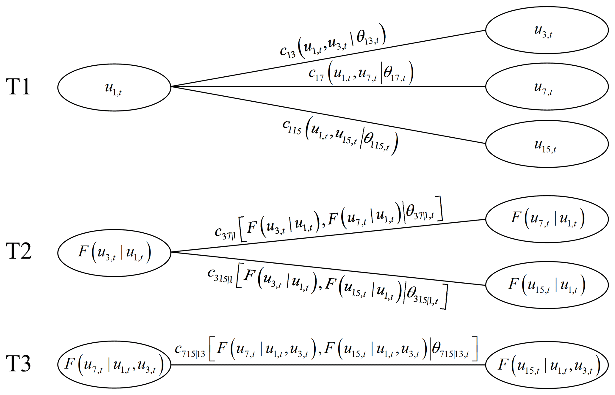
Numerous pair copula decomposition forms for a multivariate distribution are available, among which two kinds of decompositions with regular vine structures prevail in practice, namely the canonical vine (C vine) and the drawable vine (D vine; Aas et al., 2009). It is known that flood peak (e.g. Q₁) is the dominant feature quantifying a flood event as well as being the key factor in hydrologic design (Ministry of Water Resources of People's Republic of China, 1996). The C vine is more suitable when there is a key variable governing multivariate dependence (Aas et al., 2009). In this case, the C vine was employed to construct the joint distribution of $(Q_{1}, V_{3}, V_{7}, V_{15})$ , with Q₁ elected as the key variable. Thus, the density function $c (u_{1, t}, u_{3, t}, u_{7, t}, u_{15, t} | θ_{c, t})$ can be decomposed into six bivariate pair copulas as follows:

\begin{array}{l} c (u_{1, t}, u_{3, t}, u_{7, t}, u_{15, t} | θ_{c, t}) = c_{13} (u_{1, t}, u_{3, t} | θ_{13, t}) \\ \cdot c_{17} (u_{1, t}, u_{7, t} |θ_{17, t}) \cdot c_{115} (u_{1, t}, u_{15, t} |θ_{115, t}) \\ \cdot c_{37 | 1} [F (u_{3, t} | u_{1, t}), F (u_{7, t} | u_{1, t}) |θ_{37 | 1, t}] \\ \cdot c_{315 | 1} [F (u_{3, t} | u_{1, t}), F (u_{15, t} | u_{1, t}) |θ_{315 | 1, t}] \\ \cdot c_{715 | 13} [F (u_{7, t} | u_{1, t}, u_{3, t}), \\ (4) & F (u_{15, t} | u_{1, t}, u_{3, t}) | θ_{715 | 13, t}], \end{array}

where $θ_{c, t} = (θ_{13, t}, θ_{17, t}, θ_{115, t}, θ_{37 | 1, t}, θ_{315 | 1, t}, θ_{715 | 13, t})$ is the parameter vector in the C-vine copula, and

\begin{array}{l} F (u_{3, t} | u_{1, t}) = \frac{\partial C_{13} (u_{1, t}, u_{3, t} | θ_{13, t})}{\partial u_{1, t}}, \\ F (u_{7, t} | u_{1, t}) = \frac{\partial C_{17} (u_{1, t}, u_{7, t} |θ_{17, t})}{\partial u_{1, t}}, \\ F (u_{15, t} | u_{1, t}) = \frac{\partial C_{115} (u_{1, t}, u_{15, t} |θ_{115, t})}{\partial u_{1, t}}, \\ F (u_{7, t} | u_{1, t}, u_{3, t}) = \\ \frac{\partial c_{37 | 1} [F (u_{3, t} | u_{1, t}), F (u_{7, t} | u_{1, t}) |θ_{37 | 1, t}]}{\partial F (u_{3, t} | u_{1, t})}, \\ F (u_{15, t} | u_{1, t}, u_{3, t}) = \\ (5) & \frac{\partial C_{315 | 1} [F (u_{3, t} | u_{1, t}), F (u_{15, t} | u_{1, t}) |θ_{315 | 1, t}]}{\partial F (u_{3, t} | u_{1, t})} . \end{array}

Figure 3 shows the schematic decomposition of the 4-D C-vine copula as expressed by Eq. (4). It is evident that the hierarchical structure of the 4-D C-vine copula contains three trees and six edges. The first tree (T1) includes three bivariate pair copulas, i.e. $c_{13} (\cdot |θ_{13, t})$ , $c_{17} (\cdot |θ_{17, t})$ and $c_{115} (\cdot |θ_{115, t})$ , which directly act on the marginal probabilities and describe the bivariate dependencies between the key variable Q₁ and the other three variables, i.e. V₃, V₇ and V₁₅. The second tree (T2) includes two bivariate pair copulas $c_{37 | 1} (\cdot |θ_{37 | 1, t})$ and $c_{315 | 1} (\cdot |θ_{315 | 1, t})$ , which act on the conditional distribution functions with u_1, t as the conditioning variable. Finally, the third tree (T3) includes only one bivariate pair copula $c_{715 | 13} (\cdot |θ_{715 | 13, t})$ acting on conditional distribution functions with both u_1, t and u_3, t as the conditioning variables.

https://www.hydrol-earth-syst-sci.net/23/1683/2019/hess-23-1683-2019-f03

Figure 3Decomposition of the four-dimensional C-vine copula.

Download

In flood frequency analysis, the upper tail of the flood distribution deserves more attention because it allows the quantification of risks of the more serious flood events. The Gumbel–Hougaard copula, an extreme-value copula widely used in hydrology, accounts for the upper tail dependence and is well-suited to the dependence structure of a multivariate flood distribution (Salvadori et al., 2007; Zhang and Singh, 2007; Xiong et al., 2015). Consequently, the present study employed the bivariate Gumbel–Hougaard copula to construct the dynamic C-vine copula formulated by Eq. (4). The bivariate Gumbel–Hougaard copula is expressed as follows:

\begin{array}{l} C (u, v) = \exp \{- {[{(- \ln u)}^{θ_{c}} + {(- \ln v)}^{θ_{c}}]}^{1 / θ_{c}}\}, \\ (6) & θ_{c} \in [1, \infty), \end{array}

where u and v are the bivariate marginal probabilities and θ_c is the single parameter measuring the dependence strength.

Similar to the nonstationary marginal distributions, the nonstationarity of the dependence structure of $(Q_{1}, V_{3}, V_{7}, V_{15})$ was characterized by the time variations of the copula parameters in T1, T2 and T3. Both linear and exponential functions were considered to characterize the time-varying copula parameters and generally formulated as follows.

\begin{matrix} (7) & \begin{array}{ll} Linear : & θ_{c, t} = β_{0} + β_{1} {Pop}_{t} + β_{2} {RI}_{t} . \\ Exponential : & θ_{c, t} = 1 + \exp (β_{0} + β_{1} {Pop}_{t} + β_{2} {RI}_{t}) . \end{array} \end{matrix}

Here β₀, β₁ and β₂ are model parameters estimated using the MLE method (Aas et al., 2009). Here, the exponential expression in Eq. (7) was written as the sum of 1 and an exponential function of the covariates so that the domain range of the copula parameter θ_c can be satisfied under any condition. To make it easy in parameter estimation, the model parameters for each pair copula were separately estimated. The model parameters for θ_13, t, θ_17, t and θ_115, t in T1 were first estimated, and those for the remaining copula parameters $θ_{37 | 1, t}$ , $θ_{315 | 1, t}$ and $θ_{715 | 13, t}$ in T2 and T3 were then estimated in sequence. It is worth noting that these parameters can be also simultaneously estimated. These two methods could result in possible difference in parameter estimation.

The available GoF tests for vine copulas are very limited, with the probability integral transform (PIT) test appearing to be reliable (Aas et al., 2009). Under a null hypothesis of the multivariate flood variables $(Q_{1}, V_{3}, V_{7}, V_{15})$ following a given C-vine copula, the PIT converts the dependent flood variables into a new set of variables that are independent and uniformly distributed on [0, 1]⁴. The GoF of vine copulas can be obtained through determining whether the resulting variables are independent and uniform in [0, 1]. For more details of the PIT test, readers are referred to Aas et al. (2009). The best nonstationary model for each bivariate pair copula in Eq. (4) was chosen from the nonstationary models generally expressed by Eq. (7) in terms of the AICc value.

3.2 Multivariate hydrologic design under nonstationary conditions

3.2.1 Average annual reliability for multivariate flood events

The AAR introduced by Read and Vogel (2015) was calculated using the arithmetic-average method, thereby taking into account the reliability of each year with the same weighting factor. A safer design strategy should pay more attention to worse (i.e. lower) annual reliability; however, the arithmetic-average AAR is not capable of this function. The present study employed the geometric-average method to calculate AAR, which is dominated more by the minimum than arithmetic average and is theoretically able to yield safer design values. The geometric-average AAR is also equivalent to the metrics of the DLL (Rootzén and Katz, 2013) and ER (Liang et al., 2016; Yan et al., 2017).

Denoting $(q_{1}, v_{3}, v_{7}, v_{15})$ as a given multivariate flood event, its exceedance probability p_t, which is the occurrence probability of a more dangerous multivariate event than $(q_{1}, v_{3}, v_{7}, v_{15})$ in a specific hazard scenario, would vary from year to year under nonstationary conditions. The AAR for $(q_{1}, v_{3}, v_{7}, v_{15})$ was calculated by the geometric-average method as follows:

\begin{matrix} (8) & AAR (q_{1}, v_{3}, v_{7}, v_{15}) = {[\prod_{t = T_{1}}^{T_{2}} (1 - p_{t})]}^{\frac{1}{T_{2} - T_{1} + 1}}, \end{matrix}

where T₁ and T₂ stand for the beginning year and ending year of the operation of an assumed hydraulic structure, respectively, $T_{2} - T_{1} + 1$ is the length of the design life period of the hydraulic structure, and 1−p_t measures the annual reliability of the given multivariate flood event $(q_{1}, v_{3}, v_{7}, v_{15})$ at time t.

3.2.2 Exceedance probabilities of multivariate flood events

The present study characterized AAR by considering three widely used definitions of the exceedance probabilities of the multivariate flood event $(q_{1}, v_{3}, v_{7}, v_{15})$ , i.e. the OR, AND and Kendall cases (Salvadori and De Michele, 2004, 2010; Favre et al., 2004; Salvadori et al., 2007, 2016; Vandenberghe et al., 2011). The OR case for $(q_{1}, v_{3}, v_{7}, v_{15})$ defines the case under which at least one of the flood features exceeds the prescribed threshold. The exceedance probability in the OR case at time t was denoted as $p_{t}^{or}$ and was calculated by the following:

\begin{array}{l} p_{t}^{or} & = P (Q_{1, t} \geq q_{1} \lor V_{3, t} \geq v_{3} \lor V_{7, t} \geq v_{7} \lor V_{15, t} \geq v_{15}) \\ (9) & = 1 - F (q_{1}, v_{3}, v_{7}, v_{15} |θ_{t}), \end{array}

where “∨” stands for the OR operator and F(⋅|θ_t) is defined in Eq. (1).

The AND case for $(q_{1}, v_{3}, v_{7}, v_{15})$ defines the case under which all of the flood features exceed the prescribed thresholds, and the corresponding exceedance probability $p_{t}^{and}$ at time t was expressed as follows:

\begin{array}{l} p_{t}^{and} = P (Q_{1, t} > q_{1} \land V_{3, t} > v_{3} \land V_{7, t} > v_{7} \land V_{15, t} > v_{15}) \\ = \int \int \int \int_{Ω^{and}} f (Q_{1, t}, V_{3, t}, V_{7, t}, V_{15, t} |θ_{t}) d Q_{1, t} \\ \cdot d V_{3, t} \cdot d V_{7, t} \cdot d V_{15, t} \\ Ω^{and} : q_{1} < Q_{1, t} < \infty, v_{3} < V_{3, t} < \infty, v_{7} < V_{7, t} < \infty, \\ (10) & v_{15} < V_{15, t} < \infty, \end{array}

where “∧” is the AND operator and f(⋅|θ_t) is defined in Eq. (2).

Under the Kendall case, the multivariate flood event $(q_{1}, v_{3}, v_{7}, v_{15})$ was first transformed into a univariate representation via Kendall's distribution function K_C(⋅) as follows:

\begin{array}{l} K_{C} (ρ_{t}) & = P [C (U_{1, t}, U_{3, t}, U_{7, t}, U_{15, t} |θ_{c, t}) \leq ρ_{t}] \\ (11) & = P [F (Q_{1, t}, V_{3, t}, V_{7, t}, V_{15, t} |θ_{t}) \leq ρ_{t}], \end{array}

where $ρ_{t} = F (q_{1}, v_{3}, v_{7}, v_{15} |θ_{t})$ is the probability level corresponding to the given flood event $(q_{1}, v_{3}, v_{7}, v_{15})$ . The exceedance probability $p_{t}^{ken}$ in the Kendall case at time t was expressed as follows:

\begin{matrix} (12) & p_{t}^{ken} = 1 - K_{C} (ρ_{t}) . \end{matrix}

For general multivariate cases, the exceedance probabilities $p_{t}^{or}$ , $p_{t}^{and}$ and $p_{t}^{ken}$ could have no analytical solutions but can be numerically estimated through the Monte Carlo method (Niederreiter, 1978; Salvadori et al., 2011, 2013). The AAR in the OR, AND and Kendall cases can be calculated by replacing the exceedance probability p_t in Eq. (8) by $p_{t}^{or}$ , $p_{t}^{and}$ and $p_{t}^{ken}$ , respectively.

3.2.3 Most-likely design event and confidence interval for multivariate hydrologic design

The methods identifying both the most-likely design event, denoted by $(z_{Q_{1}}^{*}, z_{V_{3}}^{*}, z_{V_{7}}^{*}, z_{V_{15}}^{*})$ , and the confidence interval for the multivariate hydrologic design $(z_{Q_{1}}, z_{V_{3}}, z_{V_{7}}, z_{V_{15}})$ given AAR=η are introduced below. The average annual probability density, denoted by g(⋅), of $(z_{Q_{1}}, z_{V_{3}}, z_{V_{7}}, z_{V_{15}})$ over the entire design life period from T₁ to T₂, was expressed as follows:

\begin{array}{l} g (z_{Q_{1}}, z_{V_{3}}, z_{V_{7}}, z_{V_{15}}) = \\ (13) & \frac{1}{T_{2} - T_{1} + 1} \sum_{t = T_{1}}^{T_{2}} f (z_{Q_{1}}, z_{V_{3}}, z_{V_{7}}, z_{V_{15}} |θ_{t}) . \end{array}

The probability distribution function for AAR≤η can be written as

\begin{array}{l} Φ (η) & = \underset{Ω : AAR (q_{1}, v_{3}, v_{7}, v_{15}) \leq η}{\int \int \int \int} g (q_{1}, v_{3}, v_{7}, v_{15}) \\ (14) & d q_{1} d v_{3} d v_{7} d v_{15} . \end{array}

By denoting the density function of Φ(η) as ϕ(η), the probability density of $(z_{Q_{1}}, z_{V_{3}}, z_{V_{7}}, z_{V_{15}})$ conditioned on AAR=η can be expressed as follows:

\begin{array}{l} g_{| AAR} & = η (z_{Q_{1}}, z_{V_{3}}, z_{V_{7}}, z_{V_{15}}) \\ (15) & = \frac{g (z_{Q_{1}}, z_{V_{3}}, z_{V_{7}}, z_{V_{15}})}{ϕ (η)} . \end{array}

The most-likely design event conditioned on AAR=η was theoretically written as

\begin{array}{l} (z_{Q_{1}}^{*}, z_{V_{3}}^{*}, z_{V_{7}}^{*}, z_{V_{15}}^{*}) = \\ (16) & \arg max g_{| AAR = η} (z_{Q_{1}}, z_{V_{3}}, z_{V_{7}}, z_{V_{15}}) . \end{array}

Unfortunately, the analytical solutions of both the most-likely design event $(z_{Q_{1}}^{*}, z_{V_{3}}^{*}, z_{V_{7}}^{*}, z_{V_{15}}^{*})$ and confidence interval are unavailable but can be approximately estimated through the Monte Carlo simulation method. First, the design events with sample size N conditioned on AAR=η were generated. These design events were then sorted in descending order of their multivariate probability densities, denoted by

\begin{array}{l} (z_{Q_{1}}^{1}, z_{V_{3}}^{1}, z_{V_{7}}^{1}, z_{V_{15}}^{1}), (z_{Q_{1}}^{2}, z_{V_{3}}^{2}, z_{V_{7}}^{2}, z_{V_{15}}^{2}), \dots, \\ (17) & (z_{Q_{1}}^{N c}, z_{V_{3}}^{N c}, z_{V_{7}}^{N c}, z_{V_{15}}^{N c}), \dots, (z_{Q_{1}}^{N}, z_{V_{3}}^{N}, z_{V_{7}}^{N}, z_{V_{15}}^{N}), \end{array}

where $N c = N \cdot p_{c}$ , and p_c is the critical probability level for the confidence interval. Thus, the approximate solution for $(z_{Q_{1}}^{*}, z_{V_{3}}^{*}, z_{V_{7}}^{*}, z_{V_{15}}^{*})$ is $(z_{Q_{1}}^{1}, z_{V_{3}}^{1}, z_{V_{7}}^{1}, z_{V_{15}}^{1})$ . The lower boundary for the confidence interval was expressed as follows:

\begin{matrix} (18) & \{\begin{cases} z_{Q_{1}}^{L} = \min (z_{Q_{1}}^{1}, z_{Q_{1}}^{2}, \dots, z_{Q_{1}}^{N c}) \\ z_{V_{3}}^{L} = \min (z_{V_{3}}^{1}, z_{V_{3}}^{2}, \dots, z_{V_{3}}^{N c}) \\ z_{V_{7}}^{L} = \min (z_{V_{7}}^{1}, z_{V_{7}}^{2}, \dots, z_{V_{7}}^{N c}) \\ z_{V_{15}}^{L} = \min (z_{V_{15}}^{1}, z_{V_{15}}^{2}, \dots, z_{V_{15}}^{N c}) \end{cases} . \end{matrix}

The upper boundary for the confidence interval was estimated by the following:

\begin{matrix} (19) & \{\begin{cases} z_{Q_{1}}^{U} = \max (z_{Q_{1}}^{1}, z_{Q_{1}}^{2}, \dots, z_{Q_{1}}^{N c}) \\ z_{V_{3}}^{U} = \max (z_{V_{3}}^{1}, z_{V_{3}}^{2}, \dots, z_{V_{3}}^{N c}) \\ z_{V_{7}}^{U} = \max (z_{V_{7}}^{1}, z_{V_{7}}^{2}, \dots, z_{V_{7}}^{N c}) \\ z_{V_{15}}^{U} = \max (z_{V_{15}}^{1}, z_{V_{15}}^{2}, \dots, z_{V_{15}}^{N c}) \end{cases} . \end{matrix}

3.2.4 Derivation of design flood hydrographs

In China, the design flood hydrographs for hydraulic structures are usually derived from the design flood events set against a benchmark flood hydrograph, which is chosen from the observed flood processes (Ministry of Water Resources of People's Republic of China, 1996; Xiao et al., 2009, Yin et al., 2017). For example, suppose that a flood hydrograph consists of the features of annual maximum daily discharge, 3-day flood volume, 7-day flood volume and 15-day flood volume. The four features of the benchmark flood hydrograph are denoted by $Q_{1}^{B}$ , $V_{3}^{B}$ , $V_{7}^{B}$ and $V_{15}^{B}$ , respectively. The design flood hydrograph corresponding to the multivariate hydrologic design realization $(z_{Q_{1}}, z_{V_{3}}, z_{V_{7}}, z_{V_{15}})$ can be derived by multiplying the benchmark flood hydrograph by different amplifiers, given as described below.

The amplifier K₁ for the annual maximum daily discharge was calculated by

\begin{matrix} (20) & K_{1} = \frac{z_{Q_{1}}}{Q_{1}^{B}} . \end{matrix}

The amplifier K₃₋₁ for the 3-day flood volume except for the annual maximum daily discharge was calculated by

\begin{matrix} (21) & K_{3 - 1} = \frac{z_{V_{3}} - V (z_{Q_{1}})}{V_{3}^{B} - V (Q_{1}^{B})}, \end{matrix}

where V(⋅) is the operator transforming daily discharge into flood volume. The amplifier K₇₋₃ for the 7-day flood volume except for the 3-day flood volume was calculated by

\begin{matrix} (22) & K_{7 - 3} = \frac{z_{V_{7}} - z_{V_{3}}}{V_{7}^{B} - V_{3}^{B}} . \end{matrix}

Finally, the amplifier K₁₅₋₇ for the 15-day flood volume except for the 7-day flood volume was calculated by

\begin{matrix} (23) & K_{15 - 7} = \frac{z_{V_{15}} - z_{V_{7}}}{V_{15}^{B} - V_{7}^{B}} . \end{matrix}

4 Results

4.1 Nonstationary analysis for marginal distributions

The time-varying moment model was employed to perform nonstationary analysis for each marginal distribution of the multivariate flood series $(Q_{1}, V_{3}, V_{7}, V_{15})$ of the Xijiang River. In general, the candidate distributions for all margins passed the GoF test at the 0.05 significance level. The chosen models featured with the smallest AICc values were shown in Table 2. The results indicated that the GEV distribution provided the best fit for the annual maximum daily discharge series Q₁, whereas the Gamma distribution was chosen as the theoretical distribution for the flood volume series V₃, V₇ and V₁₅. All estimated model parameters were found to be statistically significant at the 0.05 level. The 95 % uncertainty intervals for the estimated parameters were calculated by the parametric bootstrap method (Kyselý, 2009). In accordance with the modelling results, it can be seen that the location parameters μ for all flood series were nonstationary, while the scale and shape parameters were stationary. Through an exponential function, the location parameters μ referring to the means of the flood series were generally positively related to the urban population Pop, whereas they were negatively related to the reservoir index RI. This finding revealed the opposite roles played by urbanization and reservoir regulation on the flood processes of the XRB. In particular, more artificial levees were required to protect urban areas from flooding by constraining the flood flow to river channels, which resulted in increasing the river channel flood flow. The reservoirs played an active role in flood control by reducing the flood discharge downstream.

Table 2Results of nonstationary analysis for the marginal distributions of $(Q_{1}, V_{3}, V_{7}, V_{15})$ .

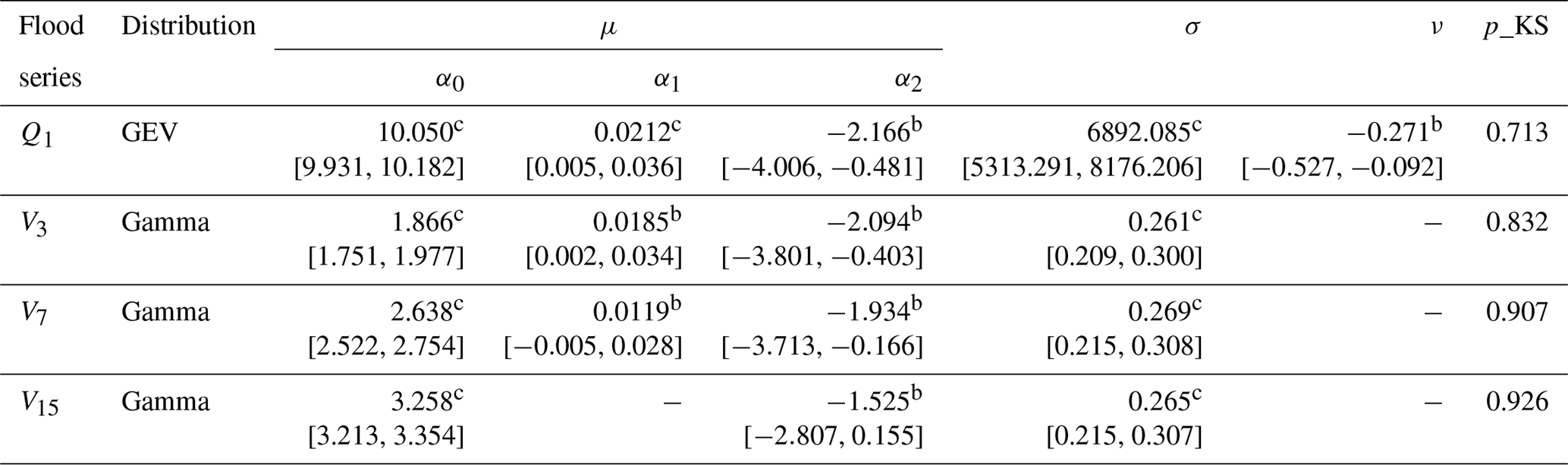
The relationships between μ and covariates were built by the exponential function in Eq. (3). α₁ and α₂ are the parameters related to urban population (Pop) and reservoir index (RI), respectively. The symbols ^a, ^b and ^c denote that the estimated model parameters are significant at the levels of 0.1, 0.05 and 0.1, respectively. The numbers in brackets are the 95 % uncertainty interval. p_KS stands for the p value of the KS test for marginal distributions.

Download Print Version | Download XLSX

More specific to each margin of $(Q_{1}, V_{3}, V_{7}, V_{15})$ , the location parameters μ of the three short-duration flood series, i.e. Q₁, V₃ and V₇, were positively linked to Pop, whereas the RI was the driving factor reducing μ for all flood series, including Q₁, V₃, V₇ and V₁₅. Owing to the difference in covariate selections, the short-duration flood series, including Q₁, V₃ and V₇, displayed asynchronous nonstationary behaviours with the long-duration flood series V₁₅ occurring in the observation period of 1951–2012. As shown in Fig. 4, Q₁, V₃ and V₇ presented significantly increasing trends during 1951–2005, particularly since the 1980s, marking the beginning of a period of rapid urbanization in China. V₁₅ tended to follow a stationary process during 1951–2005. After the two flood control reservoirs were put into operation in 2006, all flood series, including Q₁, V₃, V₇ and V₁₅, exhibited a sharp decline.

https://www.hydrol-earth-syst-sci.net/23/1683/2019/hess-23-1683-2019-f04

Figure 4Nonstationary marginal distributions during both the observation and design life periods.

Download

Table 3Results of nonstationary analysis for the dependence structure of $(Q_{1}, V_{3}, V_{7}, V_{15})$ .

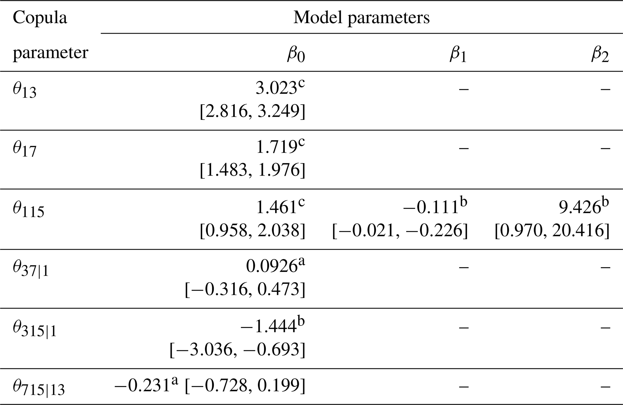
The relationships between copula parameters and covariates were built by the exponential function in Eq. (7). β₁ and β₂ are the parameters related to urban population (Pop) and reservoir index (RI), respectively. The symbols ^a, ^b and ^c denote that the estimated model parameters are significant at the levels of 0.1, 0.05 and 0.01, respectively. The numbers in brackets are the 95 % uncertainty interval.

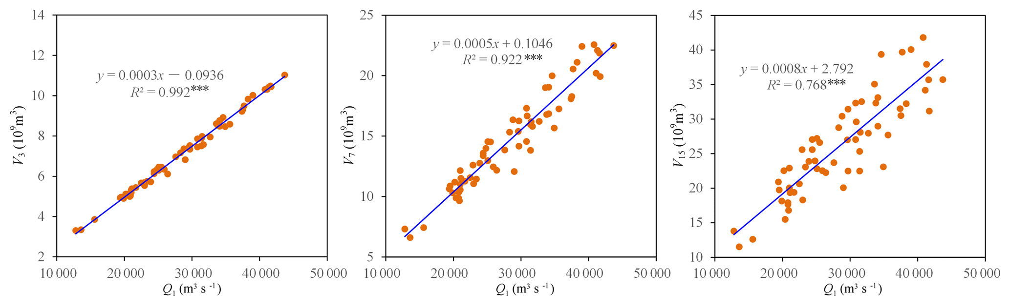
Download Print Version | Download XLSX

https://www.hydrol-earth-syst-sci.net/23/1683/2019/hess-23-1683-2019-f05

Figure 5Statistical correlations between flood peak and flood volumes. Three asterisks (***) indicate the statistical correlation at the 0.01 significance level.

Download

The predicted marginal distributions for $(Q_{1}, V_{3}, V_{7}, V_{15})$ during the design life period from 2013 to 2100 were estimated using the time-varying moment model by replacing the observed covariates for μ with those predicted. Figure 4 also shows that the mean values of Q₁, V₃ and V₇ during the design life period increased with the growth of the urban population, following which they decreased sharply in 2023 after a larger reservoir named Datengxia is expected to be put into operation. After 2023, with no more reservoirs planned, the predicted mean values of Q₁, V₃ and V₇ would be expected to reach their peaks in the mid-21th century followed by a slight declining trend because of a shrinking urban population. Since V₁₅ was only related to RI, V₁₅ would show an abrupt decline in 2023 due to the regulation of the Datengxia reservoir. In general, the predicted nonstationary marginal distributions for Q₁ and V₃ during 2013–2100 were roughly approximate to the marginal distributions under the assumption of stationarity, whereas the predicted nonstationary marginal distributions for V₇ and V₁₅ exhibited smaller mean values than those of the stationary distributions.

4.2 Nonstationary dependence structure for $(Q_{1}, V_{3}, V_{7}, V_{15})$

After estimating the nonstationary marginal distributions for $(Q_{1}, V_{3}, V_{7}, V_{15})$ , the multivariate dependence structure was constructed by the dynamic C-vine copula with Q₁ elected as the key variable. Figure 5 illustrates significant correlations between the flood peak Q₁ and the flood volumes (i.e. V₃, V₇ and V₁₅). Table 3 shows the estimation results of the dynamic C-vine copula. The PIT test for the nonstationary dependence structure of $(Q_{1}, V_{3}, V_{7}, V_{15})$ suggested a satisfactory fitting effect, and most estimated parameters were statistically significant at the 0.05 level. The results indicated that the copula parameter θ₁₁₅ for pair (Q₁, V₁₅) was found to be nonstationary and expressed as an exponential function of both the urban population Pop and reservoir index RI, whereas other copula parameters indicated stationary dependences. It was seen that the margin of Q₁ displayed asynchronous nonstationarity behaviours with V₁₅ (see Table 2 and Fig. 4). Therefore, the dependence nonstationarity of the pair (Q₁, V₁₅) could possibly be attributed to the asynchronous marginal nonstationarities.

According to the regression function, θ₁₁₅ was negatively related to Pop, whereas it was positively related to RI. In other words, growing urbanization weakened the multivariate flood dependence, whereas reservoir regulation played an opposite role, enhancing the dependence. This finding indicated that human activities, including urbanization and reservoir regulation, not only changed the statistical characteristics of the marginal distributions of $(Q_{1}, V_{3}, V_{7}, V_{15})$ but also affected the dependence of $(Q_{1}, V_{3}, V_{7}, V_{15})$ . Figure 6 shows the time variations of θ₁₁₅ during the observation period of 1951–2012 as well as during the design life period of 2013–2100. Due to reservoir regulation, θ₁₁₅ presented two obvious upward change points in both 2006 and 2023. Besides this, θ₁₁₅ also exhibited an obvious decreasing trend with urban population growth from 1951 to the mid-21th century, followed by a slight increasing trend due to a shrinking urban population. During the design life period, the predicted nonstationary θ₁₁₅ suggests a weaker dependence for $(Q_{1}, V_{3}, V_{7}, V_{15})$ than the dependence under the stationary assumption, since it is usually smaller than the stationary estimation.

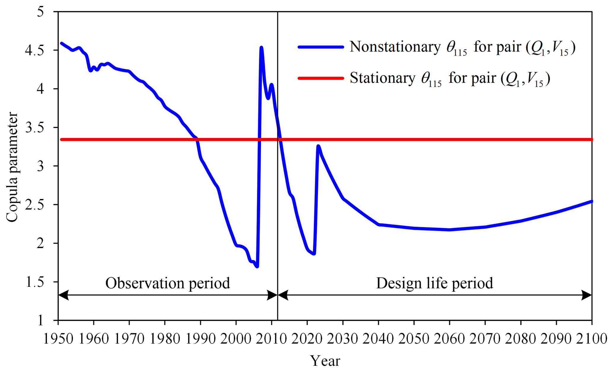
https://www.hydrol-earth-syst-sci.net/23/1683/2019/hess-23-1683-2019-f06

Figure 6Nonstationary copula parameter for pair (Q₁, V₁₅) during both the observation and design life periods.

Download

In addition, the change-point detection method based on the Cramér–von Mises statistic (Bücher et al., 2014) was employed to detect possible nonstationarities in both the marginal distributions and dependence of the multivariate flood series $(Q_{1}, V_{3}, V_{7}, V_{15})$ . Readers are referred to Bücher et al. (2014) and Kojadinovic (2017) for specific steps to implement the change-point detection. The results indicated that neither the marginal distributions nor dependence displayed change points at the 0.05 significance level (see Table 4), whereas the previous analysis suggested nonstationary margins and dependence due to the joint effects of urbanization and reservoir regulation. These aforementioned inconsistencies could be attributed to the opposite roles of urbanization and reservoir regulation on shifting of the multivariate flood distribution, with urbanization generally enlarging the mean values of the flood series and weakening their dependence and reservoir regulation, decreasing the mean values and strengthening the dependence. In other words, the nonstationarities induced by these two factors may have offset each other. As a result, the nonstationarities of $(Q_{1}, V_{3}, V_{7}, V_{15})$ might have not been captured by the statistical method based on the Cramér–von Mises statistic. This finding highlights the significance of cause–effect analysis in judging the nonstationarities of hydrologic series (Xiong et al., 2015).

Table 4Results of change-point detection for the marginal distributions and dependence of $(Q_{1}, V_{3}, V_{7}, V_{15})$ .

Download Print Version | Download XLSX

https://www.hydrol-earth-syst-sci.net/23/1683/2019/hess-23-1683-2019-f07

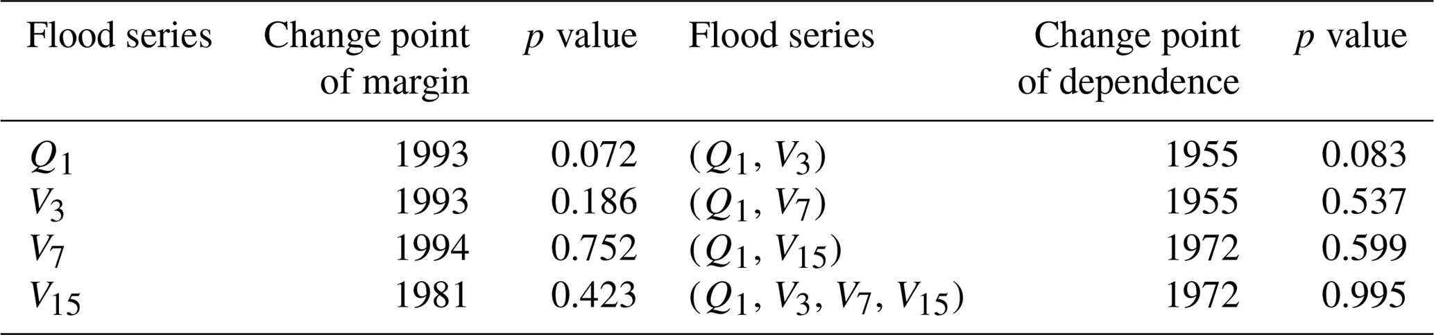
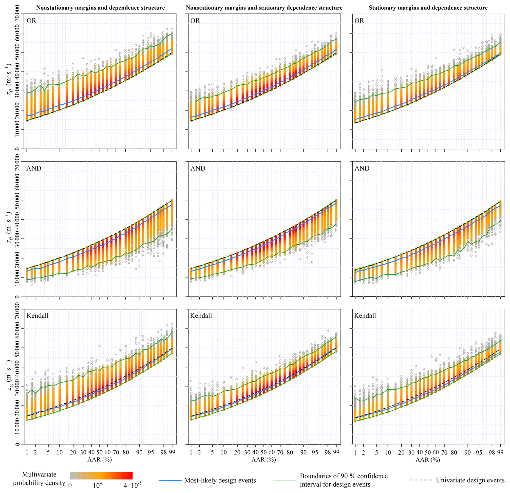
Figure 7Design values of the annual maximum daily discharge for different average annual reliability (AAR) varying from 0.01 to 0.99 under three nonstationary conditions.

Download

https://www.hydrol-earth-syst-sci.net/23/1683/2019/hess-23-1683-2019-f08

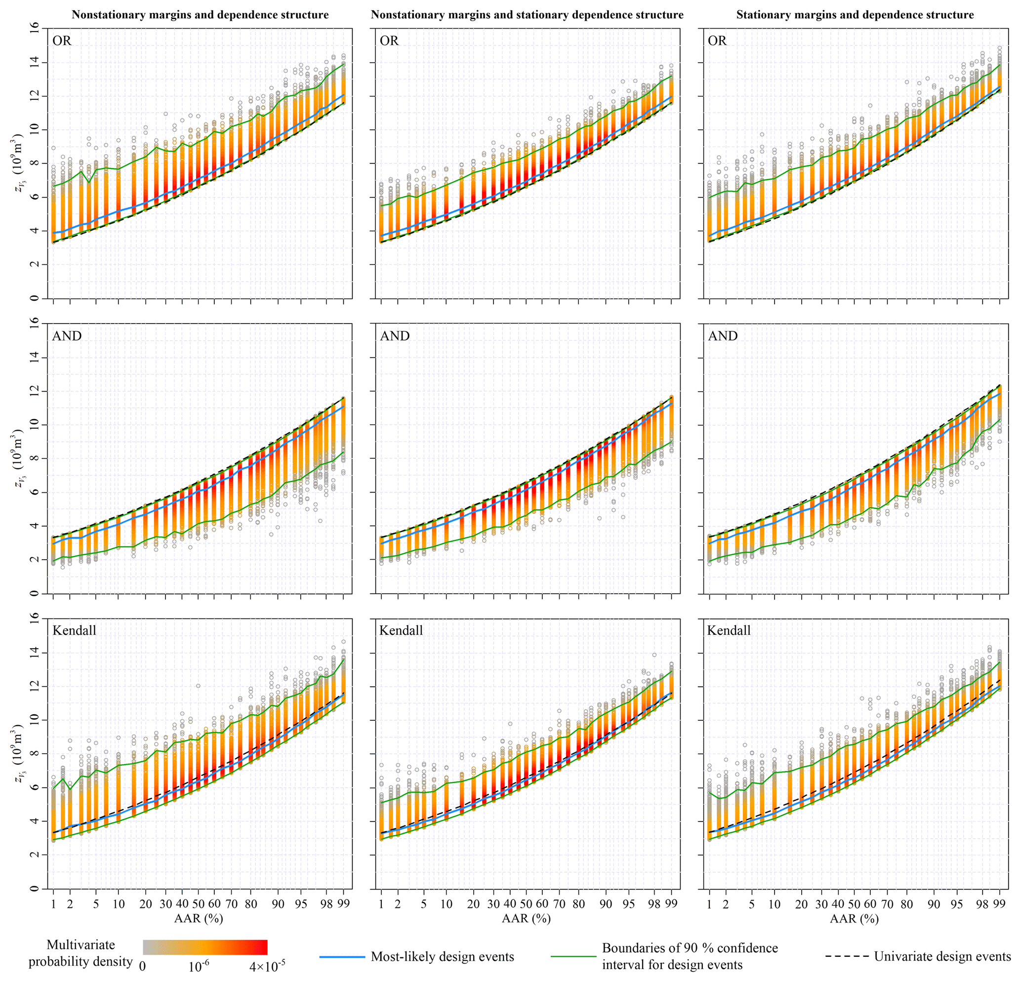
Figure 8Design values of the 3-day flood volume for different average annual reliability (AAR) varying from 0.01 to 0.99 under three nonstationary conditions.

Download

https://www.hydrol-earth-syst-sci.net/23/1683/2019/hess-23-1683-2019-f09

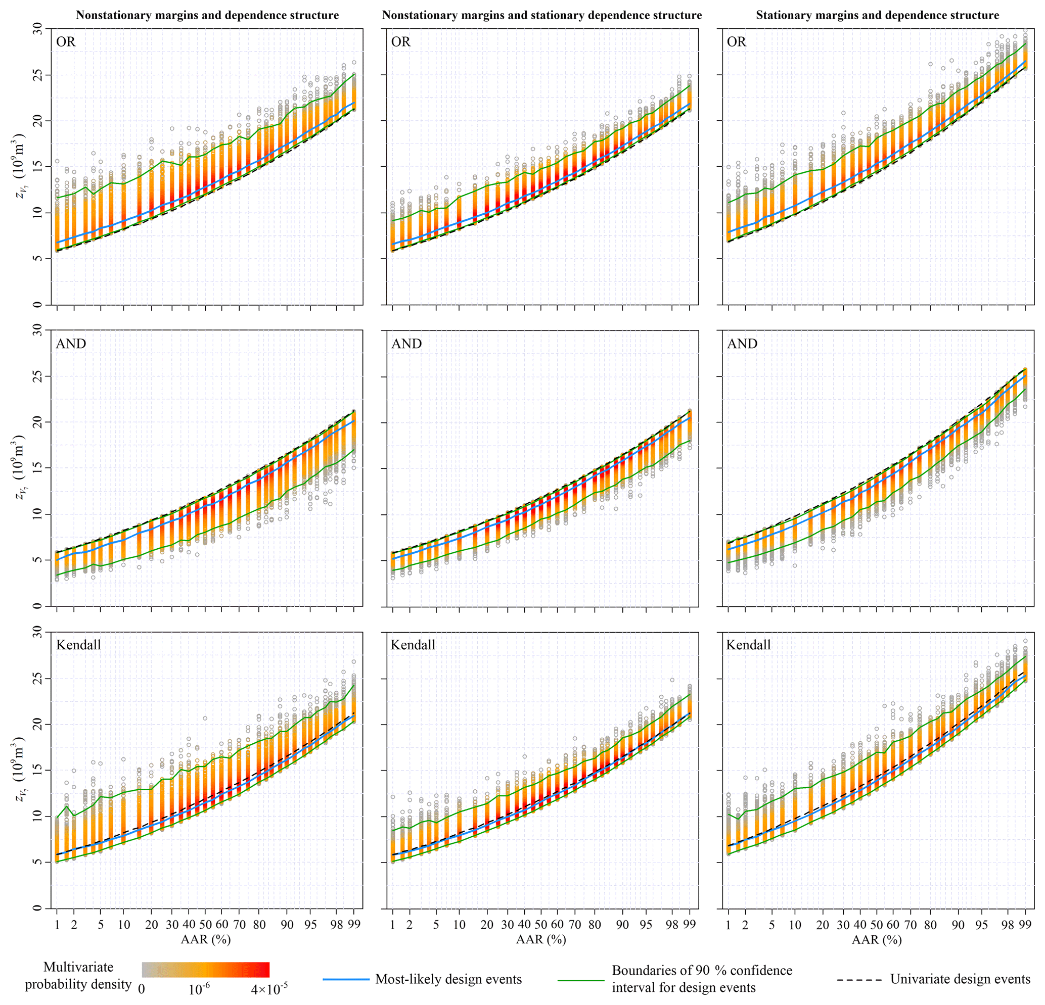
Figure 9Design values of the 7-day flood volume for different average annual reliability (AAR) varying from 0.01 to 0.99 under three nonstationary conditions.

Download

https://www.hydrol-earth-syst-sci.net/23/1683/2019/hess-23-1683-2019-f10

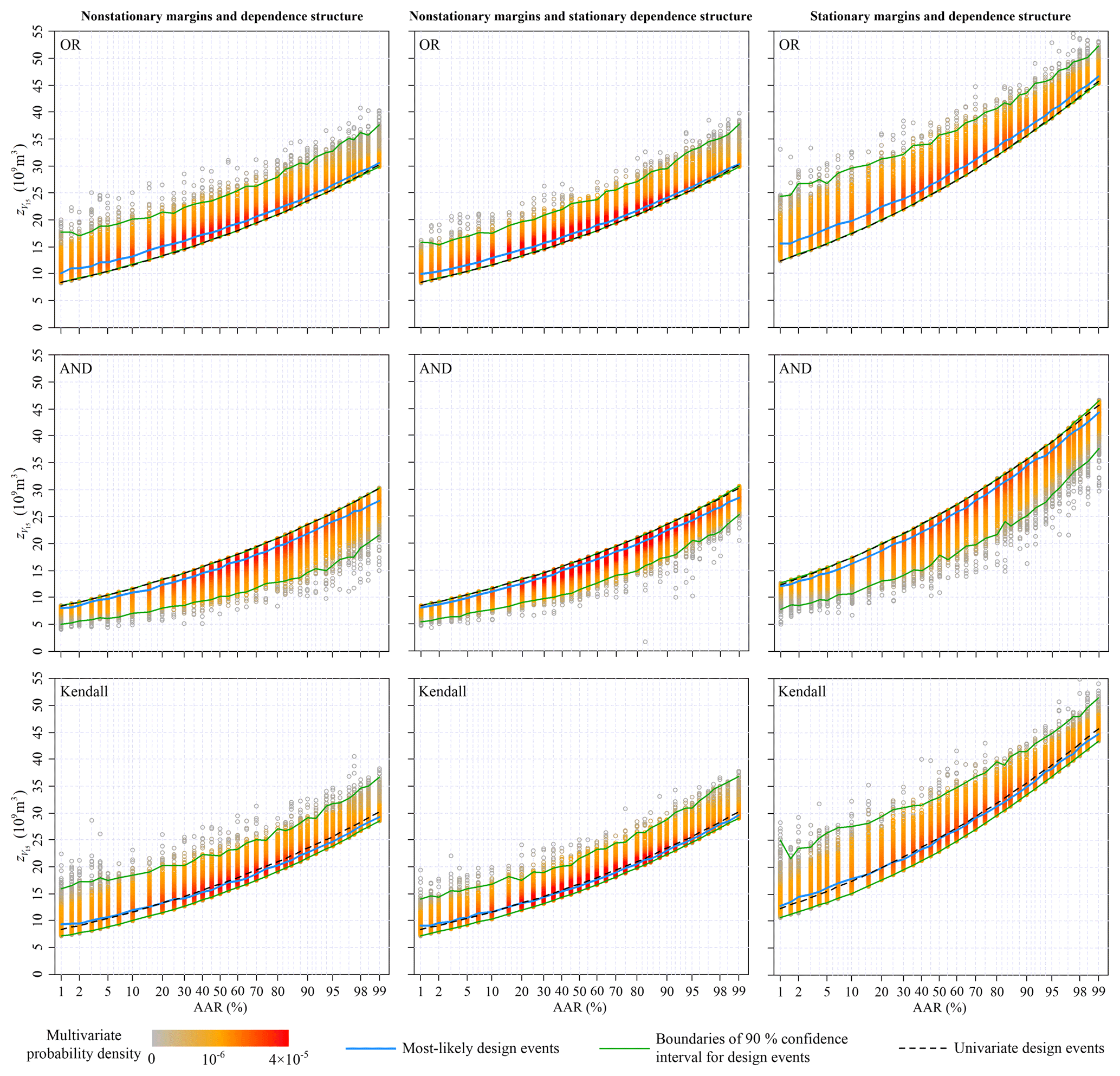
Figure 10Design values of the 15-day flood volume for different average annual reliability (AAR) varying from 0.01 to 0.99 under three nonstationary conditions.

Download

https://www.hydrol-earth-syst-sci.net/23/1683/2019/hess-23-1683-2019-f11

Figure 11Design flood hydrographs associated with OR, AND and Kendall probabilities.

Download

4.3 Multivariate hydrologic design characterized by average annual reliability

The multivariate hydrologic designs, characterized by AAR associated with the OR, AND and Kendall exceedance probabilities, were estimated from the predicted nonstationary multivariate distribution for $(Q_{1}, V_{3}, V_{7}, V_{15})$ during the design life period from 2013 to 2100. The left columns in Figs. 7–10 show the most-likely design events and the 90 % confidence intervals conditioned on the AAR varying from 0.01 to 0.99. The multivariate hydrologic design events associated with both the OR and Kendall exceedance probabilities exhibited the lower boundaries, whereas the design events associated with the AND exceedance probability exhibited the upper boundaries.

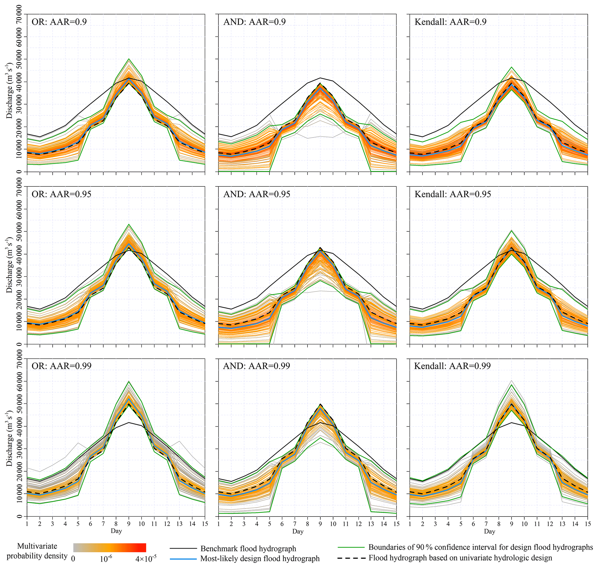
The design flood hydrographs were derived from the multivariate hydrologic designs against the benchmark flood hydrograph observed in 1988. Figure 11 shows the design flood hydrographs by setting AAR equal to 0.90, 0.95 and 0.99. For any given multivariate flood event, the corresponding OR exceedance probability was larger than that of AND, with the Kendall exceedance probability somewhere in between (Vandenberghe et al., 2011). These differences among the OR, AND and Kendall exceedance probabilities indicate the different design strategies. It must be noted that the choice of design strategy in engineering practice is usually a priori and is dependent on the specific design requirements and mechanisms of failure for hydraulic structures (Serinaldi, 2015; Salvadori et al., 2016).

We calculated the univariate hydrologic design events from the predicted marginal distributions to compare the design strategies under the multivariate framework with those under the univariate framework. Figures 7–10 show that the univariate hydrologic design events exactly constituted the lower boundaries of the multivariate hydrologic design events associated with the OR exceedance probability as well as the upper boundaries of the design events associated with the AND exceedance probability. Under a given AAR, the hydrologic designs under the univariate framework were generally smaller than the most-likely design events associated with the OR exceedance probability, whereas they were larger than those associated with the AND exceedance probability; they were most approximate to those associated with the Kendall exceedance probability. The comparisons of the flood hydrographs displayed in Fig. 11 reinforced these findings.

4.4 Impacts of multivariate nonstationarity behaviours on hydrologic design values

Section 4.1 and 4.2 show the marginal distribution and dependence structure of the multivariate flood distribution of $(Q_{1}, V_{3}, V_{7}, V_{15})$ to be nonstationary. We estimated the multivariate hydrologic design events under an assumption of stationarity to illustrate how these nonstationarities act on the multivariate hydrologic designs, i.e. both marginal distributions and the dependence structure were treated as stationary (see the right columns in Figs. 7–10). Figure 4 suggests that both the predicted nonstationary marginal distributions for Q₁ and V₃ during the design life period were approximate to the stationary marginal distributions. Therefore, the nonstationary and stationary marginal distributions yielded similar design values for $z_{Q_{1}}$ and $z_{V_{3}}$ (see Figs. 7 and 8). The predicted nonstationary distributions for both V₇ and V₁₅ indicated smaller mean values compared to those of the stationary distributions (see Fig. 4); therefore, the corresponding hydrologic design values estimated from the nonstationary marginal distributions were generally smaller than those estimated from the stationary marginal distributions (see Figs. 9 and 10).

The nonstationary multivariate flood distribution during the design life period was also predicted to exhibit a weaker dependence structure than that of the stationary distribution (see Fig. 6). The dependence nonstationarity was expected to have a much subtler effect on the multivariate hydrologic design compared to the marginal nonstationarities (Xiong et al., 2015). To illustrate the individual effect of the dependence nonstationarity on the multivariate hydrologic design, an artificial nonstationary condition for the multivariate flood distribution was set so that only the marginal nonstationarities were considered, whereas the dependence structure was treated as stationary. The results of the multivariate hydrologic design events are shown in the middle columns in Figs. 7–10. In general, the dependence nonstationarity had less of an effect on the multivariate hydrologic designs compared the marginal nonstationarities; however, some visible differences in both the 90 % confidence intervals were still identified. In summary, the nonstationary and weaker dependence structure generally suggested wider confidence intervals for the multivariate hydrologic design values.

5 Conclusion and remarks

The statistical characteristics of both the marginal distributions and the dependence structure of multivariate flood variables can vary with time under nonstationary conditions. It is possible that the multivariate flood distribution estimated from the historical information will not reflect the statistical characteristics of flooding in the future. As a result, the stationary-based hydrologic design would not be able to deal with potential hydrologic risks of hydraulic structures. It is necessary for hydrologic designers to take into account the physical driving forces (such as human activates and climate change) responsible for the nonstationarities of multivariate flood variables.

The present study introduced possible methods for addressing multivariate hydrologic design for application in engineering practice under nonstationary conditions. A dynamic C-vine copula allowing for both time-varying marginal distributions and time-varying dependence structure was developed to capture the nonstationarities of a multivariate flood distribution. The multivariate hydrologic design under nonstationary conditions was estimated by specifying the design criterion by average annual reliability. The most-likely design event and confidence interval were identified as the outcome of the multivariate hydrologic design. Multivariate flood series $(Q_{1}, V_{3}, V_{7}, V_{15})$ from the Xijiang River were chosen as a case study, with the main findings given below.

Urbanization and reservoir regulation were found to be the driving forces responsible for the nonstationarities of both the marginal distributions and dependence structure of the multivariate flood series $(Q_{1}, V_{3}, V_{7}, V_{15})$ . The growth of the urban population generally resulted in an increased mean value of the individual flood series, whereas it weakened the dependence of $(Q_{1}, V_{3}, V_{7}, V_{15})$ . The increasing reservoir index had the opposite effect on the individual flood series as well as their dependence. Under a given average annual reliability, the OR exceedance probability yielded the largest design values, followed by the Kendall and the AND exceedance probabilities. Nonstationarities in both marginal distributions and dependence structure affected the outcome of the multivariate hydrologic design. It is the marginal nonstationarities that played a dominant role in affecting the multivariate hydrologic design.

There are two remarks that can be made that are related to the practical implications of the hydrologic design methods developed in the current study that are detailed below.

The first remark relates to the length of observed flood data required for multivariate and nonstationary hydrologic designs. In theory, sufficiently long observed flood data (or other extreme-value data) are required to derive robust estimations of the distribution parameters and the correct hydrologic design values (Zheng et al., 2018). However, in reality, most data series are limited in length, thus forcing us to use what we have at hand to do research or design works without fulfilling the theoretical assumptions or requirements. Some recent studies suggested that univariate flood frequency analysis under stationary conditions usually requires flood data with a continuous period of at least 30 years (Ministry of Water Resources of People's Republic of China, 1996; Engeland et al., 2018; Kobierska et al., 2018). However, determining a definitive answer to the length of observed flood data that is required for flood frequency analysis under multivariate and/or nonstationary settings poses a challenge, since this issue has not yet been fully addressed. However, it is certain that multivariate and nonstationary hydrologic designs naturally require datasets of longer length, since they usually contain more parameters to be estimated.

The second remark related to the trade-off between reducing estimation bias and increasing model uncertainty. Nonstationary models generally improve performance in fitting observation data by reducing estimation bias (Jiang et al., 2015b), but this is usually achieved at the expense of increasing model complexity, such as adding more model parameters and introducing more nonstationary covariates, which might induce additional sources of model uncertainty (Serinaldi and Kilsby, 2015; Read and Vogel, 2016). A careful balance between the model fitting effect and the model complexity should be maintained in practice when employing multivariate and nonstationary hydrologic design by keeping in mind the following two points: (1) the multivariate and nonstationary models should remain effective but should also be kept as simple as possible to avoid overfitting, and (2) to ensure a robust relationship between the distribution parameters and the explanatory covariates, the chosen covariates should be physically related to the flood processes and supported by a well-defined cause–effect analysis.

Data availability

All the data used in this study can be requested by contacting the corresponding author Cong Jiang at jiangcong@cug.edu.cn.

Appendix A: Calculating multivariate exceedance probabilities

A1 OR exceedance probability (formulated by Eq. 9 in the paper)

Since the cumulative distribution function $F (q_{1}, v_{3}, v_{7}, v_{15} |θ_{t})$ has no analytical expression, the OR exceedance probability $p_{t}^{or}$ at time t is calculated by the Monte Carlo method as follows:

Calculate the marginal probabilities $(u_{1}, u_{3}, u_{7}, u_{15})$ of $(q_{1}, v_{3}, v_{7}, v_{15})$ .
Generate m samples $(u_{1, i}, u_{3, i}, u_{7, i}, u_{15, i})$ ( $i = 1, 2, \dots, m)$ from the C-vine copula expressed by Eq. (4).
Calculate $F (q_{1}, v_{3}, v_{7}, v_{15} |θ_{t}) = \frac{1}{m + 1} \sum_{i = 1}^{m} 1 (u_{1, i} \leq u_{1}, u_{3, i} \leq u_{3}, u_{7, i} \leq u_{7}, u_{15, i} \leq u_{15})$ .
Calculate $p_{t}^{or} = 1 - F (q_{1}, v_{3}, v_{7}, v_{15} |θ_{t})$ .

A2 AND exceedance probability (formulated by Eq. 10 in the paper)

The AND exceedance probability $p_{t}^{and}$ at time t is calculated by the Monte Carlo method as follows:

Calculate the marginal probabilities $(u_{1}, u_{3}, u_{7}, u_{15})$ of $(q_{1}, v_{3}, v_{7}, v_{15})$ .
Generate m samples $(u_{1, i}, u_{3, i}, u_{7, i}, u_{15, i})$ ( $i = 1, 2, \dots, m)$ from the C-vine copula expressed by Eq. (4).
Calculate $p_{t}^{and} = \frac{1}{m + 1} \sum_{i = 1}^{m} 1 (u_{1, i} \geq u_{1}, u_{3, i} \geq u_{3}, u_{7, i} \geq u_{7}, u_{15, i} \geq u_{15})$ .

A3 The Kendall exceedance probability (formulated by Eqs. 11 and 12 in the paper)

The Kendall exceedance probability $p_{t}^{ken}$ at time t is calculated by the Monte Carlo method as follows:

Calculate the marginal probabilities $(u_{1}, u_{3}, u_{7}, u_{15})$ of $(q_{1}, v_{3}, v_{7}, v_{15})$ .
Calculate $ρ_{t} = F (q_{1}, v_{3}, v_{7}, v_{15} |θ_{t})$ (see calculation steps 2–3 for OR exceedance probability).
Generate m samples $(u_{1, i}, u_{3, i}, u_{7, i}, u_{15, i})$ ( $i = 1, 2, \dots, m)$ from the C-vine copula expressed by Eq. (4).
For $j = 1, 2, \dots, m$ , calculate $v_{j} = \frac{1}{m + 1} \sum_{i = 1}^{m} 1 (u_{1, i} \leq u_{1, j}, u_{3, i} \leq u_{3, j}, u_{7, i} \leq u_{7, j}, u_{15, i} \leq u_{15, j})$ .
Calculate $K_{C} (ρ_{t}) = \frac{1}{m} \sum_{i = 1}^{m} 1 (v_{i} \leq ρ_{t})$ .
Calculate $p_{t}^{ken} = 1 - K_{C} (ρ_{t})$ .

Appendix B: Generating the multivariate design event samples (formulated by Eq. 17 in the paper)

To calculate the most-likely design event and confidence interval conditioned on AAR=η, we need to generate numerous multivariate design event samples by the Monte Carlo method. Here, we give the details of generating the design event samples as follows:

Define the total number of design event samples N and the initial number of the design event sample i=0.
Generate a random integer (denoted by t_r) among (T₁, T₁+1, … , T₂).
Generate a random sample $(z_{Q_{1}}, z_{V_{3}}, z_{V_{7}}, z_{V_{15}})$ following the multivariate distribution $F (z_{Q_{1}}, z_{V_{3}}, z_{V_{7}}, z_{V_{15}} |θ_{t_{r}})$ with the distribution parameter vector $θ_{t_{r}}$ .
Calculate the annual exceedance probability for each year throughout the period from T₁ to T₂.
Calculate AAR during the period from T₁ to T₂.
If $|AAR - η| < ε$ (where it is a very small value, such as 0.0001), $i = i + 1$ .
If i<N, repeat steps (2)–(6).

Author contributions

CJ and LX developed the main ideas. CJ and LY implemented the algorithms of the methods. CJ and JD collected the data used in the case study. CJ, LX and CYX prepared the paper.

Competing interests

The authors declare that they have no conflict of interest.

Acknowledgements

This research was jointly financially supported by the National Natural Science Foundation of China (NSFC grants 51809243 and 51525902), the Fundamental Research Funds for the Central Universities (grant CUG170679), the Research Council of Norway (FRINATEK Project 274310) and the “111 Project” Fund of China (B18037), all of which are greatly appreciated. The authors express their gratitude to the reviewers for their constructive comments and suggestions that have helped improve the paper.

Review statement

This paper was edited by Carlo De Michele and reviewed by four anonymous referees.

References

Aas, K., Czado, C., Frigessi, A., and Bakken, H.: Pair-copula constructions of multiple dependence, Insurance Math. Econ., 44, 182–198, https://doi.org/10.1016/j.insmatheco.2007.02.001, 2009.

Akaike, H.: A new look at the statistical model identification, IEEE Trans. Autom. Control, 19, 716–723, 1974.

Balistrocchi, M. and Bacchi, B.: Derivation of flood frequency curves through a bivariate rainfall distribution based on copula functions: application to an urban catchment in northern Italy's climate, Hydrol. Res., 48, 749–762, https://doi.org/10.2166/nh.2017.109, 2017.

Bender, J., Wahl, T., and Jensen, J.: Multivariate design in the presence of non-stationarity, J. Hydrol., 514, 123–130, https://doi.org/10.1016/j.jhydrol.2014.04.017, 2014.

Blöschl, G., Hall, J., Parajka, J., Perdigão, R. A. P., Merz, B., Arheimer, B., and Živkovic, N: Changing climate shifts timing of European floods, Science, 357, 588–590, 2017.

Bracken, C., Holman, K. D., Rajagopalan, B., and Moradkhani, H.: A Bayesian hierarchical approach to multivariate nonstationary hydrologic frequency analysis, Water Resour. Res., 54, 243–255, https://doi.org/10.1002/2017WR020403, 2018.

Bücher, A., Kojadinovic, I., Rohmer, T., and Segers, J.: Detecting changes in cross-sectional dependence in multivariate time series, J. Multivariate Anal., 132, 111–128, https://doi.org/10.1016/j.jmva.2014.07.012, 2014.

Chow, V. T.: Handbook of Applied Hydrology, McGraw-Hill, New York, 1964.

Department of Comprehensive Statistics of National Bureau of Statistics: China Compendium of Statistics 1949–2008, China Stat. Press, Beijing, 2010 (in Chinese).

Engeland, K., Wilson, D., Borsányi, P., Roald, L., and Holmqvist, E.: Use of historical data in flood frequency analysis: A case study for four catchments in Norway, Hydrol. Res., 49, 466–486, 2018,

Favre, A. C., El Adlouni, S., Perreault, L., Thiémonge, N., and Bobée, B.: Multivariate hydrological frequency analysis using copulas, Water Resour. Res., 40, W01101, https://doi.org/10.1029/2003WR002456, 2004.

Frank, J. and Massey, J. R.: The Kolmogorov-Smirnov test for goodness of fit, J. Am. Stat. Assoc., 46, 68–78, 1951.

Hawkes, P. J.: Joint probability analysis for estimation of extremes, J. Hydraul. Res., 46, 246–256, https://doi.org/10.1080/00221686.2008.9521958, 2008.

He, C.: The China Modernization Report 2013, Peking University Press, Beijing, 2014 (in Chinese).

Hurvich, C. M. and Tsai, C. L.: Regression and time series model selection in small samples, Biometrika, 76, 297–307, 1989.

Jiang, C., Xiong, L., Xu, C.-Y., and Guo, S.: Bivariate frequency analysis of nonstationary low-flow series based on the time-varying copula, Hydrol. Process., 29, 1521–1534, https://doi.org/10.1002/hyp.10288, 2015a.

Jiang, C., Xiong, L., Wang, D., Liu, P., Guo, S., and Xu, C.-Y.: Separating the impacts of climate change and human activities on runoff using the Budyko-type equations with time-varying parameters, J. Hydrol., 522, 326–338, https://doi.org/10.1016/j.jhydrol.2014.12.060, 2015b.

Kew, S. F., Selten, F. M., Lenderink, G., and Hazeleger, W.: The simultaneous occurrence of surge and discharge extremes for the Rhine delta, Nat. Hazards Earth Syst. Sci., 13, 2017–2029, https://doi.org/10.5194/nhess-13-2017-2013, 2013.

Kobierska, F., Engeland, K., and Thorarinsdottir, T.: Evaluation of design flood estimates – a case study for Norway, Hydrol. Res., 49, 450–465, 2018.

Kojadinovic, I.: npcp: Some nonparametric CUSUM tests for change-point detection in possibly multivariate observations, R Package Version 0.1-9, Vienna, Austria, available at: https://cran.r-project.org/web/packages/npcp/npcp.pdf (last access: 20 March 2019), 2017.

Kundzewicz, Z. W., Pińskwar, I., and Brakenridge, G. R.: Changes in river flood hazard in Europe: a review, Hydrol. Res., 49, 294–302, 2018.

Kwon, H.-H., Lall, U., and Kim, S.-J.: The unusual 2013–2015 drought in South Korea in the context of a multicentury precipitation record: Inferences from a nonstationary, multivariate, Bayesian copula model, Geophys. Res. Lett., 43, 8534–8544, https://doi.org/10.1002/2016GL070270, 2016.

Kyselý, J.: A cautionary note on the use of nonparametric bootstrap for estimating uncertainties in extreme-value models, J. Appl. Meteorol. Clim., 47, 3236–3251, 2009.

Li, T., Guo, S., Liu, Z., Xiong, L., and Yin, J.: Bivariate design flood quantile selection using copulas, Hydrol. Res., 48, 997–1013, 2017.

Liang, Z., Hu, Y., Huang, H., Wang, J., and Li, B.: Study on the estimation of design value under non-stationary environment, South-to-North Water Transfers, Water Sci. Technol., 14, 50–53, 2016 (in Chinese).

López, J. and Francés, F.: Non-stationary flood frequency analysis in continental Spanish rivers, using climate and reservoir indices as external covariates, Hydrol. Earth Syst. Sci., 17, 3189–3203, https://doi.org/10.5194/hess-17-3189-2013, 2013.

Loveridge, M., Rahman, A., and Hill, P.: Applicability of a physically based soil water model (SWMOD) in design flood estimation in eastern Australia, Hydrol. Res., 48, 1652–1665, 2017.

Milly, P., Betancourt, J., Falkenmark, M., Hirsch, R., Kundzewicz, Z., Lettenmaier, D., and Stouffer, R.: Climate change – Stationarity is dead: Whither water management?, Science, 319, 573–574, https://doi.org/10.1126/science.1151915, 2008.

Ministry of Water Resources of People's Republic of China: Design Criterion of Reservoir Management, Chin. Water Resour. and Hydropower Press, Beijing, 1996 (in Chinese).

Niederreiter, H.: Quasi-Monte Carlo methods and pseudo-random numbers, B. Am. Math. Soc., 197, 957–1041, 1978.

Obeysekera, J. and Salas, J.: Quantifying the uncertainty of design floods under nonstationary conditions, J. Hydrol. Eng., 19, 1438–1446, https://doi.org/10.1061/(ASCE)HE.1943-5584.0000931, 2014.

Obeysekera, J. and Salas, J.: Frequency of recurrent extremes under nonstationarity, J. Hydrol. Eng., 21, 04016005, https://doi.org/10.1061/(ASCE)HE.1943-5584.0001339, 2016.

Olsen, J. R., Lambert, J. H., and Haimes, Y. Y.: Risk of extreme events under nonstationarity conditions, Risk Anal., 18, 497–510, https://doi.org/10.1111/j.1539-6924.1998.tb00364.x, 1998.

Parey, S., Hoang, T. T. H., and Dacunha-Castelle, D.: Different ways to compute temperature return levels in the climate change context, Environmetrics, 21, 698–718, https://doi.org/10.1002/env.1060, 2010.

Qi, W. and Liu, J.: A non-stationary cost-benefit based bivariate extreme flood estimation approach, J. Hydrol., 557, 589–599, https://doi.org/10.1016/j.jhydrol.2017.12.045, 2017.

Quessy, J., Saïd, M., and Favre, A. C.: Multivariate Kendall's tau for change-point detection in copulas, Can. J. Stat., 41, 65–82, https://doi.org/10.1002/cjs.11150, 2013.

Read, L. K. and Vogel, R. M.: Reliability, return periods, and risk under nonstationarity, Water Resour. Res., 51, 6381–6398, https://doi.org/10.1002/2015WR017089, 2015.

Read, L. K. and Vogel, R. M.: Hazard function analysis for flood planning under nonstationarity, Water Resour. Res., 52, 4116–4131, https://doi.org/10.1002/2015WR018370, 2016.

Requena, A. I., Mediero, L., and Garrote, L.: A bivariate return period based on copulas for hydrologic dam design: accounting for reservoir routing in risk estimation, Hydrol. Earth Syst. Sci., 17, 3023–3038, https://doi.org/10.5194/hess-17-3023-2013, 2013.

Rootzén, H. and Katz, R. W.: Design Life Level: Quantifying risk in a changing climate, Water Resour. Res., 49, 5964–5972, https://doi.org/10.1002/wrcr.20425, 2013.

Rosner, A., Vogel, R. M., and Kirshen, P. H.: A risk-based approach to flood management decisions in a nonstationary world, Water Resour. Res., 50, 1928–1942, https://doi.org/10.1002/2013WR014561, 2014.

Salas, J. D. and Obeysekera, J.: Revisiting the concepts of return period and risk for nonstationary hydrologic extreme events, J. Hydrol. Eng., 19, 554–568, https://doi.org/10.1061/(ASCE)HE.1943-5584.0000820, 2014.

Salvadori, G. and De Michele, C.: Frequency analysis via copulas: theoretical aspects and applications to hydrological events, Water Resour. Res., 40, W12511, https://doi.org/10.1029/2004WR003133, 2004.

Salvadori, G. and De Michele, C.: Multivariate multiparameter extreme value models and return periods: A copula approach, Water Resour. Res., 46, W10501, https://doi.org/10.1029/2009WR009040, 2010.

Salvadori, G., De Michele, C., Kottegoda, N. T., and Rosso, R.: Extremes in Nature: An Approach Using Copulas, Springer, Dordrecht, the Netherlands, 2007.

Salvadori, G., De Michele, C., and Durante, F.: On the return period and design in a multivariate framework, Hydrol. Earth Syst. Sci., 15, 3293–3305, https://doi.org/10.5194/hess-15-3293-2011, 2011.

Salvadori, G., Durante, F., and De Michele, C.: Multivariate return period calculation via survival functions, Water Resour. Res., 49, 2308–2311, https://doi.org/10.1002/wrcr.20204, 2013.

Salvadori, G., Durante, F., Tomasicchio, G. R., and D'Alessandro, F.: Practical guidelines for the multivariate assessment of the structural risk in coastal and off-shore engineering, Coastal Eng., 95, 77–83, https://doi.org/10.1016/j.coastaleng.2014.09.007, 2015.

Salvadori, G., Durante, F., De Michele, C., Bernardi, M., and Petrella, L.: A multivariate Copula-based framework for dealing with Hazard Scenarios and Failure Probabilities, Water Resour. Res., 52, 3701–3721, https://doi.org/10.1002/2015WR017225, 2016.

Salvadori, G., Durante, F., Michele, C. D., and Bernardi, M.: Hazard assessment under multivariate distributional change-points: Guidelines and a flood case study, Water, 10, 751–765, https://doi.org/10.3390/w10060751, 2018.

Sarhadi, A., Burn, D. H., Ausín, M. C., and Wiper, M. P.: Time-varying nonstationary multivariate risk analysis using a dynamic Bayesian copula, Water Resour. Res., 52, 2327–2349, https://doi.org/10.1002/2015WR018525, 2016.

Serinaldi, F.: Dismissing return periods!, Stoch. Env. Res. Risk. A., 29, 1179–1189, https://doi.org/10.1007/s00477-014-0916-1, 2015.

Serinaldi, F. and Kilsby, C. G.: Stationarity is undead: Uncertainty dominates the distribution of extremes, Adv. Water Resour., 77, 17–36, https://doi.org/10.1016/j.advwatres.2014.12.013, 2015.

Shafaei, M., Fakheri-Fard, A., Dinpashoh, Y., Mirabbasi, R., and De Michele, C.: Modeling flood event characteristics using D-vine structures, Theor. Appl. Climatol., 130, 713–724, https://doi.org/10.1007/s00704-016-1911-x, 2017.

Sklar, M.: Fonctions de Répartition a n Dimensions et Leurs Marges, 8 pp., Univ. Paris, Paris, 1959.

Strupczewski, W. G., Singh, V. P., and Feluch, W.: Non-stationary approach to at-site flood frequency modeling I. Maximum likelihood estimation, J. Hydrol., 248, 123–142, https://doi.org/10.1016/S0022-1694(01)00397-3, 2001.

Vandenberghe, S., Verhoest, N. E. C., Onof, C., and De Baets, B.: A comparative copula – based bivariate frequency analysis of observed and simulated storm events: A case study on Bartlett – Lewis modeled rainfall, Water Resour. Res., 47, W07529, https://doi.org/10.1029/2009WR008388, 2011.

Vezzoli, R., Salvadori, G., and De Michele, C.: A distributional multivariate approach for assessing performance of climate-hydrology models, Sci. Rep., 7, 12071, https://doi.org/10.1038/s41598-017-12343-1, 2017.

Villarini, G., Serinaldi, F., Smith, J. A., and Krajewski, W. F.: On the stationarity of annual flood peaks in the Continental United States during the 20th Century, Water Resour. Res., 45, W08417, https://doi.org/10.1029/2008WR007645, 2009.

Vogel, R. M.: Reliability indices for water supply systems, J. Water Res. Pl., 113, 563–579, https://doi.org/10.1061/(ASCE)0733-9496(1987)113:4(563), 1987.

Vogel, R. M., Yaindl, C., and Walter, M.: Nonstationarity: Flood magnification and recurrence reduction factors in the United States, J. Am. Water Resour. As., 47, 464–474, https://doi.org/10.1111/j.1752-1688.2011.00541.x, 2011.

Volpi, E. and Fiori, A.: Design event selection in bivariate hydrological frequency analysis, Hydrolog. Sci. J., 57, 1506–1515, https://doi.org/10.1080/02626667.2012.726357, 2012.

Xiao, Y., Guo, S., Liu, P., Yan, B., and Chen, L.: Design flood hydrograph based on multicharacteristic synthesis index method, J. Hydrol. Eng., 14, 1359–1364, https://doi.org/10.1061/(ASCE)1084-0699(2009)4:12(1359), 2009.

Xiong, L. and Guo, S.: Trend test and change-point detection for the annual discharge series of the Yangtze River at the Yichang hydrological station, Hydrolog. Sci. J., 49, 99–112, https://doi.org/10.1623/hysj.49.1.99.53998, 2004.

Xiong, L., Jiang, C., Xu, C.-Y., Yu, K.-X., and Guo, S.: A framework of changepoint detection for multivariate hydrological series, Water Resour. Res., 51, 8198–8217, https://doi.org/10.1002/2015WR017677, 2015.

Xu, B., Xie, P., Tan, Y., Li, X., and Liu, Y.: Analysis of flood returning to main channel influence on the flood control ability of Xijiang River, Journal of Hydroelectric Engineering, 33, 65–72, 2014 (in Chinese).

Yan, L., Xiong, L., Guo, S., Xu, C.-Y., Xia, J., and Du, T.: Comparison of four nonstationary hydrologic design methods for changing environment, J. Hydrol., 551, 132–150, https://doi.org/10.1016/j.jhydrol.2017.06.001, 2017.

Yang, T., Shao, Q., Hao, Z., Chen, Xi., Zhang, Z., Xu, C.-Y., and Sun, L.: Regional frequency analysis and spatio-temporal pattern characterization of rainfall extremes in the Pearl River Basin, China, J. Hydrol., 380, 386–405, https://doi.org/10.1016/j.jhydrol.2009.11.013, 2010.

Yin, J., Guo, S., Liu, Z., Chen, K., Chang, F., and Xiong, F.: Bivariate seasonal design flood estimation based on copulas, J. Hydrol. Eng., 22, 05017028, https://doi.org/10.1061/(ASCE)HE.1943-5584.0001594, 2017.

Zhang, L. and Singh, V. P.: Trivariate flood frequency analysis using the Gumbel–Hougaard copula, J. Hydrol. Eng., 12, 431–439, https://doi.org/10.1061/(ASCE)1084-0699(2007)12:4(431), 2007.

Zheng, F., Westra, S., and Sisson, S. A.: Quantifying the dependence between extreme rainfall and storm surge in the coastal zone, J. Hydrol., 505, 172–187, https://doi.org/10.1016/j.jhydrol.2013.09.054, 2013.

Zheng, F., Westra, S., Leonard, M., and Sisson, S. A.: Modeling dependence between extreme rainfall and storm surge to estimate coastal flooding risk, Water Resour. Res., 50, 2050–2071, https://doi.org/10.1002/2013WR014616, 2014.

Zheng, F., Leonard, M., and Westra, S.: Efficient joint probability analysis of flood risk, J. Hydroinform., 17, 584–597, 2015.

Zheng, F., Leonard, M., and Westra, S.: Application of the design variable method to estimate coastal flood risk, J. Flood Risk Manag., 10, 522–534, https://doi.org/10.1111/jfr3.12180, 2017.

Zheng, F., Tao, R., Maier, H. R., See, L., Savic, D., Zhang, T., Chen, O., Assumpção, T. H., Yang, P., Heidari, B., Rickermann, J., Minsker, B., Bi, W., Cai, X., Solomatine, D., and Popescu, I.: Crowdsourcing methods for data collection in geophysics: State of the art, issues, and future directions, Rev. Geophys., 56, 698–740, https://doi.org/10.1029/2018RG000616, 2018.

Articles

Short summary

We present the methods addressing the multivariate hydrologic design applied to the engineering practice under nonstationary conditions. A dynamic C-vine copula allowing for both time-varying marginal distributions and a time-varying dependence structure is developed to capture the nonstationarities of multivariate flood distribution. Then, the multivariate hydrologic design under nonstationary conditions is estimated through specifying the design criterion by average annual reliability.

Multivariate hydrologic design methods under nonstationary conditions and application to engineering practice

3.1 Probability distribution of the nonstationary multivariate flood series

3.1.1 Nonstationary marginal distributions based on the time-varying moment model

3.1.2 Nonstationary dependence structure based on the dynamic C-vine copula

3.2 Multivariate hydrologic design under nonstationary conditions

3.2.1 Average annual reliability for multivariate flood events

3.2.2 Exceedance probabilities of multivariate flood events

3.2.3 Most-likely design event and confidence interval for multivariate hydrologic design

3.2.4 Derivation of design flood hydrographs

4.1 Nonstationary analysis for marginal distributions

4.2 Nonstationary dependence structure for Q1,V3,V7,V15

4.3 Multivariate hydrologic design characterized by average annual reliability

4.4 Impacts of multivariate nonstationarity behaviours on hydrologic design values

A1 OR exceedance probability (formulated by Eq. 9 in the paper)

A2 AND exceedance probability (formulated by Eq. 10 in the paper)

A3 The Kendall exceedance probability (formulated by Eqs. 11 and 12 in the paper)

4.2 Nonstationary dependence structure for $(Q_{1}, V_{3}, V_{7}, V_{15})$