the Creative Commons Attribution 4.0 License.
the Creative Commons Attribution 4.0 License.
 | 15 Jan 2019
Influence of input and parameter uncertainty on the prediction of catchment-scale groundwater travel time distributions
Falk Heße
Rohini Kumar
Olaf Kolditz
Thomas Kalbacher
Sabine Attinger
Groundwater travel time distributions (TTDs) provide a robust description of the subsurface mixing behavior and hydrological response of a subsurface system. Lagrangian particle tracking is often used to derive the groundwater TTDs. The reliability of this approach is subjected to the uncertainty of external forcings, internal hydraulic properties, and the interplay between them. Here, we evaluate the uncertainty of catchment groundwater TTDs in an agricultural catchment using a 3-D groundwater model with an overall focus on revealing the relationship between external forcing, internal hydraulic properties, and TTD predictions. Eight recharge realizations are sampled from a high-resolution dataset of land surface fluxes and states. Calibration-constrained hydraulic conductivity fields (Ks fields) are stochastically generated using the null-space Monte Carlo (NSMC) method for each recharge realization. The random walk particle tracking (RWPT) method is used to track the pathways of particles and compute travel times. Moreover, an analytical model under the random sampling (RS) assumption is fit against the numerical solutions, serving as a reference for the mixing behavior of the model domain. The StorAge Selection (SAS) function is used to interpret the results in terms of quantifying the systematic preference for discharging young/old water. The simulation results reveal the primary effect of recharge on the predicted mean travel time (MTT). The different realizations of calibration-constrained Ks fields moderately magnify or attenuate the predicted MTTs. The analytical model does not properly replicate the numerical solution, and it underestimates the mean travel time. Simulated SAS functions indicate an overall preference for young water for all realizations. The spatial pattern of recharge controls the shape and breadth of simulated TTDs and SAS functions by changing the spatial distribution of particles' pathways. In conclusion, overlooking the spatial nonuniformity and uncertainty of input (forcing) will result in biased travel time predictions. We also highlight the worth of reliable observations in reducing predictive uncertainty and the good interpretability of SAS functions in terms of understanding catchment transport processes.


Travel/transit time distributions (TTDs) of groundwater provide a description of how aquifers store and release water and pollutants under external forcing conditions, which has significant implications for interdisciplinary environmental studies. For example, remarkable time lags of the reaction of streamflow with outer forcings and considerable amounts of “old water” (i.e., water with an age of decades or longer) in streamflow have been observed in many studies (Howden et al., 2010; Stewart et al., 2012). Moreover, the legacy nitrogen in groundwater storage may dominate the annual nitrogen loads in agricultural basins (Van Meter et al., 2017; Van Meter et al., 2016; Wang et al., 2016). Groundwater TTDs offer important insights into the vulnerability of aquifers to pollution spreading, and they are critically important for the environmental assessment of non-point-source agricultural contamination (Böhlke, 2002; Böhlke and Denver, 1995; Eberts et al., 2012; Molnat and Gascuel-Odoux, 2002). TTDs shed light on the quantification of the long-term influence of agricultural contamination, which is crucial for water quality and sustainability.
The accurate quantification of groundwater travel time at a regional scale is extremely challenging. A primary difficulty is that the complex geometric, topographic, meteorologic, and hydraulic properties of hydrologic systems control the flow and mixing processes and therefore define the unique shape of the TTD (Engdahl et al., 2016; Hale and McDonnell, 2016; Leray et al., 2016). The other difficulty is that the groundwater system is intricately and tightly coupled to land surface hydrologic processes. The fundamental characteristics and the coupled nature determine the response of a catchment to outer forcings such as anthropogenic climate change, artificial abstraction, and agricultural and chemical contamination (Heße et al., 2017; Tetzlaff et al., 2014; van der Velde et al., 2015).
The techniques for determining groundwater TTDs can be categorized into two groups: geochemical approaches and numerical modeling approaches (McCallum et al., 2014). In geochemical approaches, the lumped parameter models are often used to interpret the catchment-scale observation of an environmental tracer concentration. Environmental tracer datasets can be divided into those representing the concentration distribution of young water (e.g., 3H, SF6, 85K, and CFCs) and those representing the concentration distribution of old water (e.g., 36Cl, 4He, 39Ar, and 14C). Additionally, the analytical StorAge Selection (SAS) function is a cutting-edge tool for characterizing transport processes in lumped, time-varying hydrologic systems at the hillslope/catchment scale (Botter et al., 2011; Danesh-Yazdi et al., 2018; Harman, 2015; Rinaldo et al., 2011; Van Der Velde et al., 2012). This framework provides a clear distinction between the travel time (the time spent by a water parcel or a solute from its entrance to the control volume until its exit) and the residence time (the age of the water parcel or the solute existing in the control volume at a particular time). The SAS function has been successfully applied to interpret environmental tracer data through some assumptions of the mixing mechanism (Benettin et al., 2015, 2017). However, analytical approaches fall short in representing the dispersion of transport processes caused by catchment heterogeneity. Strong heterogeneity leads to significant aggregation error of mean travel times (MTTs) when using analytical models to interpret the tracer data (Kirchner, 2016; Stewart et al., 2017).
In contrast to such an analytical approach, physically based numerical models can explicitly describe the geometry, topography, and geological structures, and they can represent the flow paths of individual water particles. Physically based numerical models are structurally complex and computationally expensive and often have more parameters than lumped parameter models do. These models can be classified as Eulerian approaches or Lagrangian approaches (Leray et al., 2016). The Eulerian approach directly solves the partial differential equations (PDEs) derived from mass conservation with “age mass” as the primary variable (Engdahl et al., 2016; Ginn, 2000; Goode, 1996). The Lagrangian approach, including the smoothed particle hydrodynamics (SPH) approach and the random walk particle tracking (RWPT) approach, is numerically robust and less restrictive on time-step size in solving advection-dominated problems (Tompson and Gelhar, 1990). Consequently, Lagrangian methods are more promising in simulating complex real-world transport processes, as they avoid spurious mixing error in grid-fixed Eulerian methods (Benson et al., 2017). Therefore, the Lagrangian approach has been widely used to simulate large-scale reactive transport and biogeochemical problems (Park et al., 2008; Selle et al., 2013; de Rooij et al., 2013).
A reliable application of groundwater transport modeling is subject to many sources of uncertainty, including measurement, model structural, and parameter uncertainty (Beven, 1993). Specifically, the reliability of model prediction suffers from the uncertainty of external forcings, the uncertainty of internal hydraulic characteristics, and the interplay between them (Ajami et al., 2007). The spatially sparse measurements of recharge lead to a biased characterization of spatiotemporal patterns of recharge (Cheng et al., 2017; Healy and Scanlon, 2010). On the other hand, the spatial scarcity of hydrogeological data always hampers the right characterization of aquifer properties such as porosity and permeability, thus allowing a range of various realistic parameter values. The best-fit parameter may suffer from a fitting error caused by overparameterization and equifinality (Schoups et al., 2008). Such biased parameters cause uncertain predictions because parameter error may compensate for model structural defects (Doherty, 2015). Accordingly, predictive uncertainty can be hardly assessed in a precise way.
Biased characterization of the hydrodynamic system and oversimplified assumptions will lead to a problematic prediction of TTDs. Many past studies offer insights into the influence of recharge and hydrogeological configuration on the prediction of TTDs. For example, some research studies have been devoted to the development of analytical solutions for the idealized catchment (or aquifer) under some essential assumptions and simplifications (Engdahl et al., 2016; Haitjema, 1995; Leray et al., 2016; Neuman, 1972). Among them, Haitjema (1995) derived an analytical solution in an idealized groundwatershed under steady-state conditions and the Dupuit–Forchheimer assumption and found that the groundwater mean travel time appears to be only dependent on recharge, saturated aquifer thickness, and porosity, provided that the hydraulic conductivity is locally homogeneous. Basu et al. (2012) evaluated analytical, GIS, and numerical approaches for the prediction of groundwater TTDs and found that the simulated TTDs show a moderate difference. Many recent studies have reported the dependency of transient TTDs on the temporal variability of input forcings (Benettin et al., 2015; Kaandorp et al., 2018; Remondi et al., 2018; Yang et al., 2018), but the dependency of TTDs (as well as SAS functions) on the spatial variability of input forcings has rarely been studied.
Although studies on catchment-scale groundwater TTDs are numerous, comprehensive uncertainty analysis that aims to unveil the different roles of external forcing and internal hydrostratigraphic structure using both a numerical model and SAS functions is scarce. In this regard, two important questions are the following. (1) How does the uncertainty of recharge (including its spatial nonuniformity) and hydraulic conductivities affect the TTD predictions in a mesoscale agricultural catchment, provided that the model is constrained to reality and groundwater head observations? (2) How does the uncertainty of inputs (forcings) and parameters influence the prediction of systematic preference for young/old water?
In this paper, we aim to answer these questions through a detailed (uncertainty) analysis of an example application in a mesoscale real-world catchment. In doing so, we establish a detailed groundwater model coupled to a random walk particle tracking system for predicting groundwater TTDs. The OpenGeoSys (OGS) groundwater model is used to simulate the groundwater flow, while the input forcing is fed by the mesoscale hydrologic model (mHM) via the mHM-OGS coupling interface (Jing et al., 2018a). The numerical model follows the steady-state assumption of groundwater flow systems. This assumption is made because at the regional scale, the groundwater flow process has a much larger timescale than that of the high-frequency oscillation of recharge, which essentially dampens the effect of recharge oscillation (Leray et al., 2016). An ensemble of simulations using multiple recharge realizations and multiple equifinal hydraulic conductivity (Ks) fields is established. An analytical model is used as a reference for unveiling the mixing mechanism of the system. The StorAge Selection function is also used to interpret the simulation results of the numerical model, with an overall aim to quantify the predictive uncertainty of systematic preference for young/old water.
The candidate site in this paper is the Nägelstedt catchment, located in central Germany (see Fig. 1). With an area of approximately 850 km2, the Nägelstedt catchment is a headwater catchment of the Unstrut river. The terrain elevation of this area varies from 164 m to 516 m a.m.s.l. (above mean sea level). It is a subcatchment of the Unstrut basin, one of the most intensively used agricultural regions in Germany. About 88 % of the land in this site is marked as arable land, which is significantly higher than the average level of Thuringian land (Wechsung et al., 2008). The agricultural nitrogen input has varied over the years and locations, from 5–24 kg ha−1 in the soils of the lowlands to 2–30 kg ha−1 in the feeding area (Wechsung et al., 2008). The mean annual precipitation is approximately 660 mm.
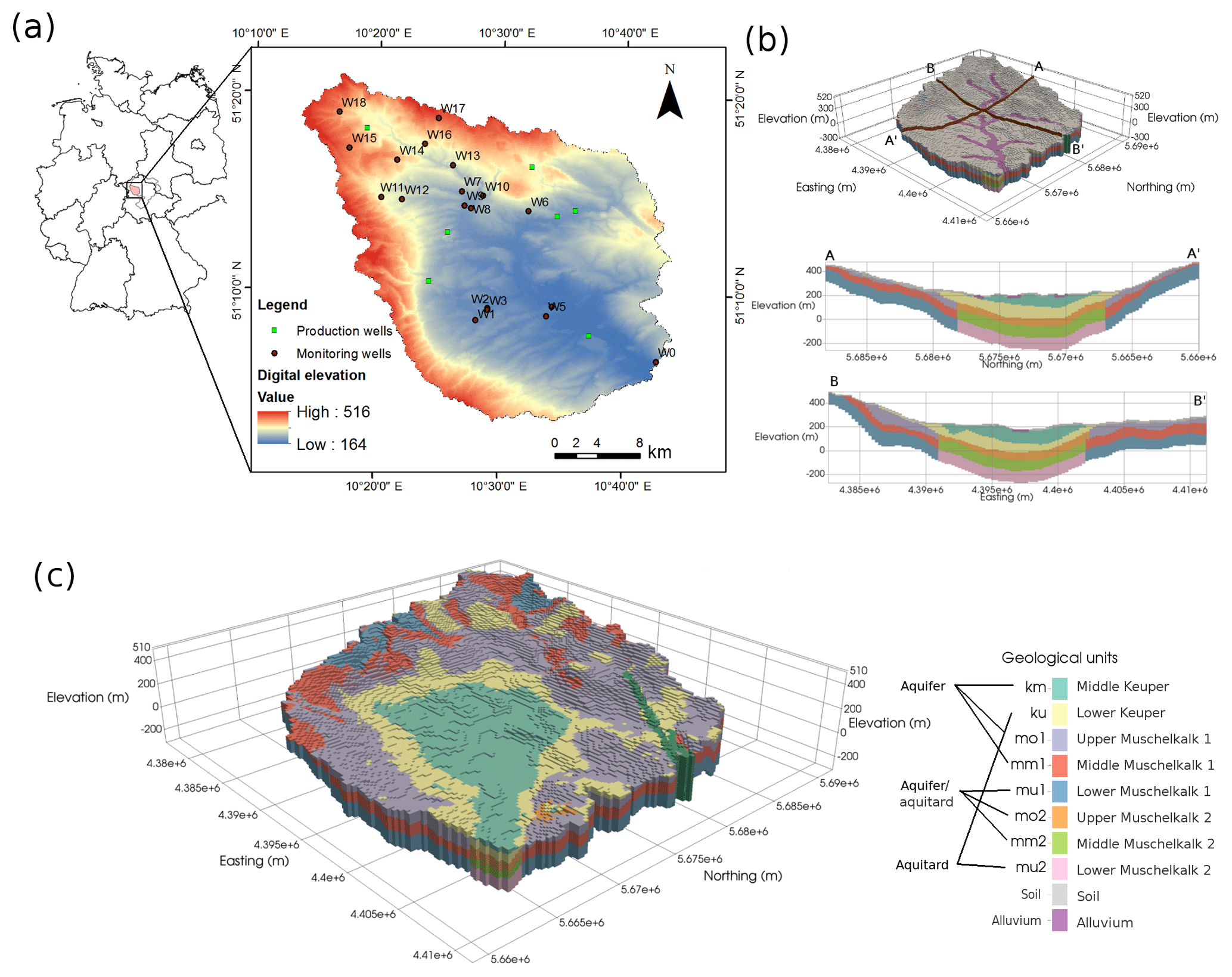
Figure 1The Nägelstedt catchment used as the test catchment for this study (Jing et al., 2018a). (a) An overview of the Nägelstedt catchment and the locations of the monitoring wells used in this study. (b) 3-D view highlighting the arrangement of alluvium and soil and cross-sectional view of the study area. (c) 3-D view highlighting the zonation of the sedimentary aquifer–aquitard system. Note that the Muschelkalk layers (mo, mm, and mu) are divided into more permeable subunits (mo1, mm1, and mu1) and less permeable subunits (mo2, mm2, and mu2).
The dominating sediment in the study area is the Muschelkalk (Middle Triassic). The Muschelkalk has an overall thickness of about 220 m, and it has been divided into three subgroups according to mineral composition: Upper Muschelkalk (mo), Middle Muschelkalk (mm), and Lower Muschelkalk (mu). The Upper Muschelkalk (mo) is mainly composed of limestone, marlstone, and claystone, and it forms fractured aquifers (Jochen et al., 2014; Kohlhepp et al., 2017; Seidel, 2003). The Middle Muschelkalk (mm) deposits are composed of evaporites, including dolomite marlstone, gypsum, dolomite limestone, and eroded salt layers. The Lower Muschelkalk (mu) is composed of massive limestone (Jochen et al., 2014; McCann, 2008; Seidel, 2003). The Muschelkalk formation consists of limestone sediments, which may form fractured and karst aquifers. A recent study demonstrated that karstification and the development of conduits are limited at the base of the Upper Muschelkalk at the Hainich critical zone in the Nägelstedt catchment (Kohlhepp et al., 2017). In the middle of the study area, Keuper deposits, including Middle Keuper (km) and Lower Keuper (ku), overlay the Muschelkalk formation. The Lower Keuper formation forms the low permeable aquitard on top of the Upper Muschelkalk aquifer (Kohlhepp et al., 2017; Seidel, 2003). Lithologically, the Muschelkalk aquifer system is a “layer-cake” aquifer system that contains interbedded marlstone aquitards (Aigner, 1982; Kohlhepp et al., 2017; Merz, 1987).
Eighteen monitoring wells distributed in this area are used to calibrate the model (Fig. 1a, in which well W0 is abandoned in this study due to the proximity to the outer edge). The geological layers to which the wells belong are listed as follows: five wells in Middle Keuper (km), four in Lower Keuper (ku), six in Upper Muschelkalk (mo), two in Middle Muschelkalk (mm), and one in alluvium.
3.1 Numerical model
We use the mHM-OGS coupled model, proposed by Jing et al. (2018a), to simulate terrestrial hydrological processes. This coupled model was developed for extending the predictive capability of mHM from land surface processes to the subsurface flow and transport processes. Specifically, mHM (Kumar et al., 2013; Samaniego et al., 2010) is used to partition water budget components, while the OGS porous media simulator (Kolditz et al., 2012) is used to compute groundwater flow and transport processes by using mHM-generated recharge as driving forces. For details on the mHM-OGS coupled model, please refer to Jing et al. (2018a).
The catchment water storage is conceptually partitioned into soil zone storage and deep groundwater storage; the two corresponding components are computed by mHM and OGS, respectively. The soil-zone dynamics of TTD has been well studied using mHM in a previous work (Heße et al., 2017). Hence, in this paper, we perform explicit forward modeling of the saturated-zone TTD through a 3-D OGS groundwater model by using the mHM-generated recharge as the external forcing.
In this study, we focus on the travel times in the saturated zone. Saturated groundwater flow is characterized by the continuity equation and Darcy's law:
where S is the specific storage coefficient in confined aquifers, or the specific yield in unconfined aquifers (1 / L); ψp is the pressure head in the porous medium (L); t is the time (T); q is the specific discharge or the Darcy velocity (LT−1); qs is the general source/sink term (T−1); Ks is the saturated hydraulic conductivity tensor (LT−1); and z is the vertical coordinate (L).
We use the RWPT method to track the particle movement. The RWPT method is embedded in the source codes of OGS (Kolditz et al., 2012; Park et al., 2008). Derived from stochastic physics, RWPT is under the assumption that the advection process is deterministic and the diffusion–dispersion process is stochastic. The theoretical background of the RWPT method is described in detail in Appendix A.
3.2 Numerical model setup
3.2.1 Boundary conditions
The steady-state model configuration is achieved using a temporally averaged recharge of the simulated daily recharges over a long period (1955–2005). The gridded recharges estimated by mHM are interpolated and then assigned to each grid node on the upper surface of the OGS mesh using a bilinear interpolation approach. No-flow boundaries are assumed at the outer edges that are defined by catchment divides, except for the northwestern and northeastern edges, where fixed-head boundaries are applied (Wechsung et al., 2008). The streams are assigned with fixed-head boundaries, wherein the heads are equal to the long-term-averaged water levels. For the steady-state system and the one-way coupled model, the baseflow component generated by OGS proves to be consistent with the baseflow estimated by mHM, implying that the water budget in the subsurface system is essentially closed (Jing et al., 2018a). Neumann boundaries are prescribed for seven drinking water production wells. However, the amount of pumping makes up only around 3 % of the total amount of outflow, and it therefore has a marginal influence on the water budget (Wechsung et al., 2008).
3.2.2 Modeling procedures
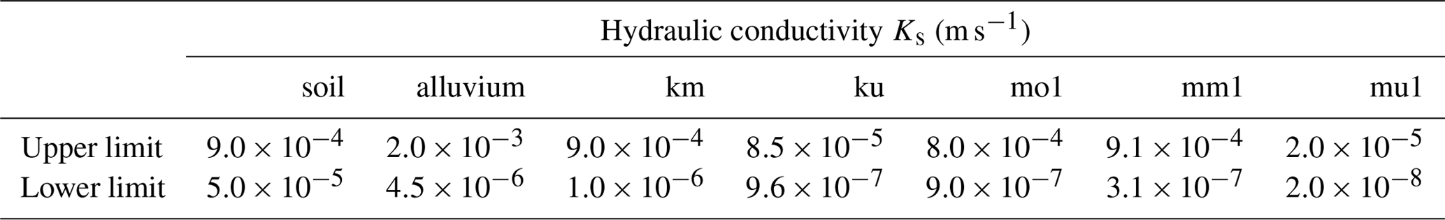
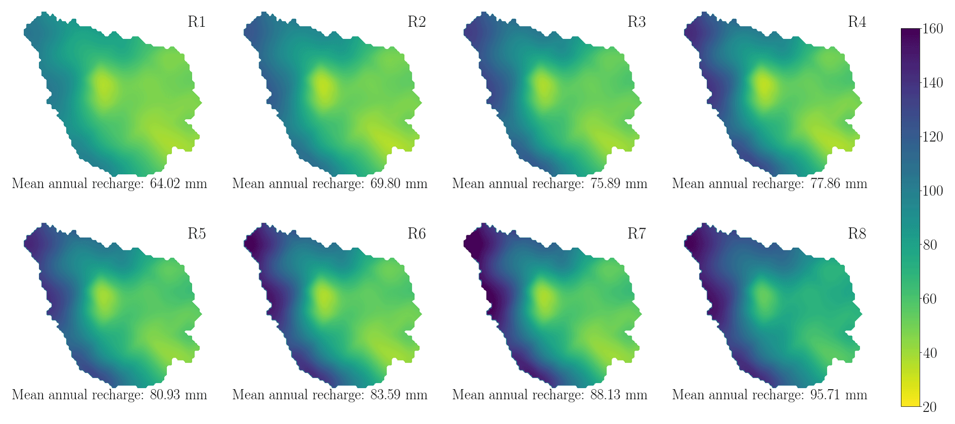
Figure 2Recharge realizations used in this study (unit: mm). They were sampled from a high-resolution dataset of land surface fluxes for Germany (Zink et al., 2017).
The numerical experiment to explore the uncertainty of TTDs is performed through the following workflow.
-
Eight spatially distributed recharge realizations are sampled from a high-resolution dataset of land surface fluxes for Germany, in which mHM is used to simulate land surface hydrological processes. The details of the dataset and the sampling method are described in the following section.
-
For each recharge realization, a series of equally probable realizations of Ks fields are generated using the null-space Monte Carlo (NSMC) method.
The NSMC method takes advantage of the hybrid Tikhonov–TSVD (truncated singular value decomposition) method in the PEST parameter estimation code to produce Monte Carlo realizations of parameters (Doherty and Hunt, 2010; Tonkin and Doherty, 2009). This approach is able to efficiently generate an ensemble of parameter fields that are conditioned to expert knowledge and measurements. Here, the observations of groundwater levels from 18 spatially distributed monitoring wells are used to calibrate the OGS model (the locations of monitoring wells are illustrated in Fig. 1a). Before generating parameter sets, we calibrate the model to obtain the best-fit hydraulic conductivities, as well as a covariance matrix of the parameter probability distributions. On the basis of this information, many fully distributed Ks fields are randomly generated from a uniform distribution of hydraulic conductivity values (Doherty, 2015). As shown in Table 1, the range of hydraulic conductivities is predefined based on values obtained from a geological survey (Wechsung et al., 2008). As a result, a total of 400 parameter sets conditioned on both observations and reality are generated for the uncertainty analysis.
-
In each parameter realization, a large number of particles are injected through the top surface of the groundwater model. The spatial density of particles is proportional to the spatially distributed recharge rates.
To accurately interpret the travel time distribution, a large number of particles (e.g., approximately 80 000 particles in the case study) is released into the top surface of the groundwater model. The released particles serve as samples of water parcels for deriving their travel time distributions. In doing so, the density of particles is set proportional to the recharge at the corresponding grid cell (Fig. 3). Each particle tracer represents a volumetric recharge rate of around 700 m3 year−1.
-
An ensemble of forward simulations using the RWPT method is performed over all realizations of Ks fields.
In each realization of the ensemble parameter sets, forward simulations of particle tracking are performed. In this study, we focus on the predictive uncertainty within the convection process. Therefore, the molecular diffusion coefficients are universally set to 0 for all ensemble simulations. The porosity of the study domain is set to 0.2 universally. Through the above procedures, the flow paths and the corresponding residence times can be fully traced in the model at random times and locations, facilitating the detailed characterization of TTDs.
In parallel to this analysis, a sensitivity analysis for the spatial variability of recharge is also performed. Two different recharge scenarios are compared for this purpose: (1) the spatially distributed recharge generated by mHM and (2) the uniform recharge that is equal to the spatial average of the distributed recharge. Other parameters, including the porosity and the hydraulic conductivity, remain identical in these two recharge scenarios.
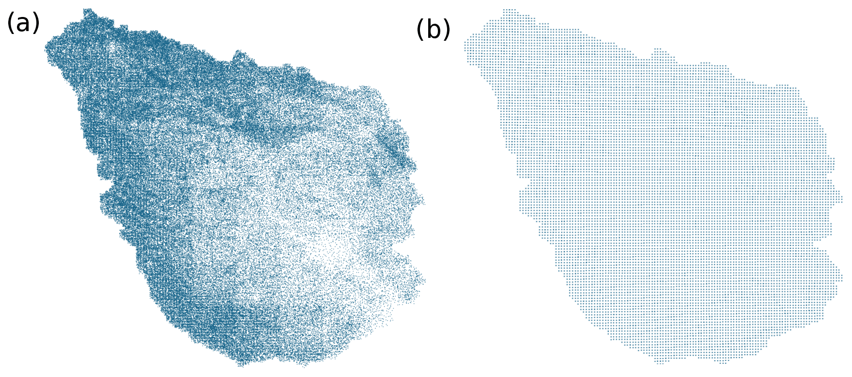
Figure 3Two different spatial distributions of particle tracers for the RWPT method. (a) The mass-weighted distribution of particles based on the recharge estimated by mHM. This is the default spatial pattern of particle tracers in this study. (b) The uniformly distributed particle tracers used in the uniform recharge scenario.
3.2.3 Recharge realizations
A high-resolution dataset of land surface fluxes and states across Germany is used for sampling recharge scenarios. This dataset was established on the basis of a daily simulation with 4 km spatial resolution using mHM for a time span of 60 years (1951–2010) (Zink et al., 2017). This dataset consists of an ensemble (100 realizations) of land surface variables, including evapotranspiration, groundwater recharge, soil moisture, and discharge, with a spatial resolution of 4 km. A total of 100 realizations of land surface states are all conditioned on the observed daily discharge, and each of them has been derived by incorporating the uncertainty of parameterization caused by the heterogeneity of geometry, topography, and geology. The modeled datasets are further validated against observation-based evapotranspiration and soil moisture data from eddy covariance stations (Heße et al., 2017). The derived recharges show a good correspondence to the estimation from the Hydrologic Atlas of Germany (Zink et al., 2017).
Eight representative recharge realizations (R1–R8) are sampled from 100 realizations for this study to save computational time. To enhance the representativeness of the samples, the 100 recharge realizations are sorted in an ascending order by their spatial averages. The selected recharge realizations are uniformly sampled from the sorted recharge realizations. In doing so, the maximum and minimum recharges are included in the samples such that the whole range of recharge realizations is fully covered.
3.2.4 3-D stratigraphic model
A 3-D stratigraphic mesh is established on the basis of hydrogeological characterizations elaborated in Sect. 2 (Fig. 1). This mesh is based on data obtained from the Thuringian State office for the Environment and Geology (TLUG) and its generation is described in Fischer et al. (2015). The structured mesh is composed of 310 599 nodes (132 rows, 140 columns, and 82 vertical layers). The 3-D cell size of 250, 250, and 10 m in the x, y, and z directions is used in this study. Based on the German stratigraphy (Menning, 2002), the Middle Muschelkalk, the Upper Muschelkalk, the Lower Keuper, and the Middle Keuper outcrop in the Nägelstedt catchment. Accordingly, a stratigraphic aquifer system with 10 geological units is set up. The uppermost 10 m of the mesh has been separated as a soil layer, while an alluvium layer consisting of high-permeability sandy gravel is set at the nodes beneath and near streams (Fig. 1). Each of the Muschelkalk layers is further divided into two categories: the more permeable parts (mo1, mm1, and mu1) and the less permeable parts (mo2, mm2, and mu2) (see Fig. 1). For each of the Muschelkalk units, the permeability of the less permeable part is tied to the corresponding more permeable part with a factor of 0.1. The equivalent porous medium approach is applied to characterize the karst aquifer of the Upper Muschelkalk (mo). This approach translates the parameters describing highly heterogeneous hydraulic properties at the point scale into the equivalent homogeneous medium at the regional scale to avoid adding redundant parameters and therefore avoid overfitting.
3.2.5 Parameter uncertainty

Figure 4Box-plot of stochastically generated hydraulic conductivity (Ks) for each geological layer in eight recharge realizations. Note that the parameters mo2, mm2, and mu2 are not shown in this figure because the less permeable subunits of the Muschelkalk (mo2, mm2, and mu2) are tied with the respective more permeable subunits (mo1, mm1, and mu1) with a factor of 0.1.
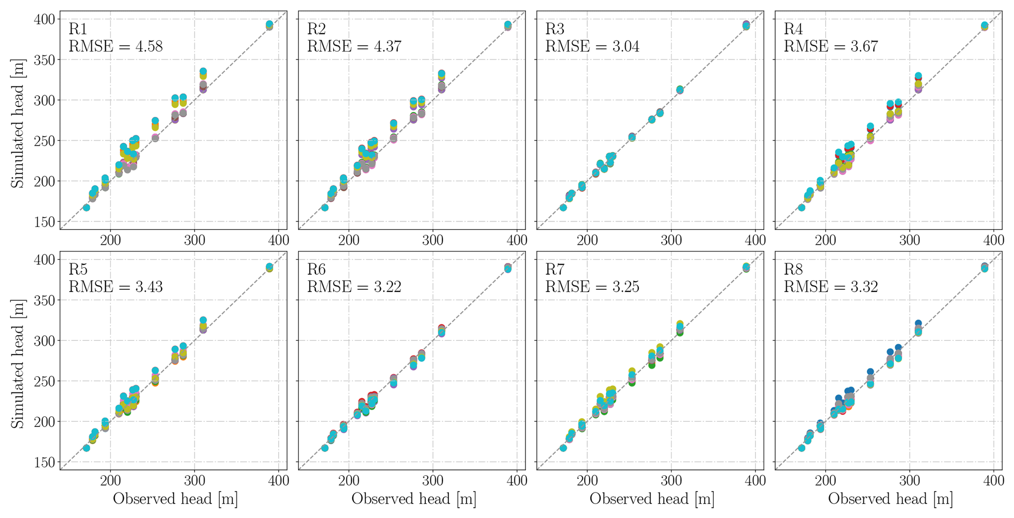
Figure 5Observed and simulated groundwater heads for each parameter and recharge realization. The results of 400 realizations (R1K1–R8K50) are categorized by recharge realization and shown in different panels.
Multiple calibration-constrained Ks fields were stochastically generated for each recharge realization. Figure 4 shows the box-plot of generated hydraulic conductivities in all realizations categorized by geological unit. The hydraulic conductivity of the Lower Muschelkalk (mu) has the highest uncertainty (10−8–10−5 m s−1) because the conductivity of mu is insensitive to groundwater head observations, given that it is the deepest geological layer and that no monitoring well is located in this layer (Table B1). The other parameters fluctuate moderately and are constrained within 1 order of magnitude in most of the recharge realizations. Hydraulic conductivities of several permeable layers (mo, mm, alluvium, and soil) increase from R1 to R8, which is not surprising because the hydraulic conductivity increases with increasing recharge and constant groundwater head. Moreover, the hydraulic conductivities of the above layers are roughly linearly correlated with the corresponding recharge in each recharge realization. Figure 5 shows the simulated and observed groundwater heads for all 400 realizations. All of the 400 realizations are well constrained to observations, with the root mean square error (RMSE) of groundwater level residuals being lower than 4.6 m in all of the considered recharge realizations.
3.3 Theory of analytical StorAge Selection function
The travel time is defined as the time spent by a moving element (either a water particle or a solute) in a control volume of a hydrologic system. In principle, the control volume can be defined at arbitrary spatial scales (i.e., from the molecular scale to the regional scale). Considering a hydrologic system in which the input flux (J) and the output fluxes () are known, each parcel of water within the system is tagged using its current age τ. The age-ranked storage is defined as the mass of water in the system with age τ<T. The backward form of the master equation (ME) for TTD in a control volume can be expressed as follows (Botter et al., 2011; Harman, 2015; Van Der Velde et al., 2012):
with boundary condition , where T is the residence time of the oldest water parcel in storage ST; t is the chronological time; is the cdf of the backward travel time distribution of output flux Qj; J(t) is the input flux at time t; and Qj(t) is the output flux at time t. Specifically in this study, J is the groundwater recharge, and Q is composed of two components: the stream baseflow and the abstraction at production wells.
The SAS function describes the fraction of water parcels leaving the control volume at time t, which is selected from the age-ranked storage ST. Following the above definition, the SAS function can be linked with the backward travel time distribution (Harman, 2015)
for . ΩQ is the cumulative form of the SAS function.
Three instances of SAS functions using gamma distribution are shown in Fig. 9a. In case the age distribution of each outflow is uniformly selected from all water storages with various ages, the outflux TTDs turn into a random sample of the storage residence time distribution (RTD). The random sampling (RS) is equivalent to the uniform SAS function (Fig. 9a). Many past studies have also considered the random sampling as a proper description of the sampling behavior for heterogeneous catchments (Benettin et al., 2015; Cartwright and Morgenstern, 2015; Heße et al., 2017). Equation (4) in this case has the analytical solution (Danesh-Yazdi et al., 2018; Harman, 2015)
where pS(T,t) is the pdf of the residence time distribution and S(t) is the storage at time t. Specifically, in the case of a steady-state hydrodynamic system, Eq. (5) is further simplified into an exponential form:
Equation (6) is the analytical solution of backward TTD under the RS assumption.
In the idealized saturated groundwater aquifer, Eq. (6) is equivalent to the analytical solution derived by Haitjema (1995). Based on the Dupuit–Forcheimer assumption, Haitjema (1995) derived a formula about the frequency distribution of residence time:
provided that nH∕J is constant over the entire domain, the recharge is spatially uniform, and the aquifer is locally homogeneous, where n is the porosity, H is the saturated aquifer thickness, and is the weighted mean travel time in the aquifer.
3.4 Linking the SAS functions to the physically based numerical model
Danesh-Yazdi et al. (2018) developed an approach to link the analytical SAS functions to the fully distributed numerical model. Although differing in numerical model and particle tracking scheme, we apply the same approach to link the SAS functions and the numerical model in this study. Equation (3) under the steady-state condition can be further simplified as
By combining Eqs. (4) and (9), the age-ranked storage ST can be calculated directly under the steady-state assumption:
Combining Eq. (10) with Eq. (4), the SAS function can be directly computed from the simulated backward TTD using the numerical model.
3.5 Predictive uncertainty of TTDs
The theoretical framework of predictive uncertainty in this paper is based on Doherty (2015). As indicated in Bayes' theorem, the parameters of a model retain uncertainty, given that they have been adjusted to best-fit values achieved during calibration. Nevertheless, the uncertainty of parameters is subject to constraints. One of the constraints resides in the fixed adjustable range of parameters, in which expert knowledge must be respected. Another constraint is exerted by the parameterization process.
While the computationally expensive Bayesian approach offers a complete theoretical framework for predictive uncertainty evaluation, practical modeling efforts are often based on model calibration and a subsequent analysis of error or uncertainty in post-calibration predictions (Doherty, 2015). Ideally, the best-fit parameters achieved through calibration can reduce the predictive error to a minimum, with the minimum predictive error being the inherent uncertainty. However, the best-fit parameter is always biased from the true parameter because the essential imperfection of the model may facilitate or hamper the achievement of the minimum. Therefore, the motivation of uncertainty analysis in this study is to quantify and minimize the predictive uncertainty of travel time distributions, given that the parameters are plausible and that the model can reproduce well the groundwater heads.
For the sake of clarity, we number the recharge realizations from R1 (with the lowest recharge rate) to R8 (with the highest recharge rate). For each recharge realization, 50 Ks fields are numbered from K1 to K50. Accordingly, R1K1 represents Ks field K1 in recharge realization R1.
4.1 Uncertainty of TTD predictions

Figure 63-D view of flow pathlines of some particles in realization R5K1. Note that only a limited number of particle pathlines are displayed here.
Flow paths of particle tracers in a random parameter realization (R5K1) are displayed in Fig. 6, serving as a visual reference for the regional groundwater flow pattern and the residence time distributions. In this realization, the deep low-permeability geological layers (e.g., mm2 and mu2) act as low-permeability aquitards. Therefore, the majority of streamlines do not enter these geological layers (Fig. 6).
Figure 7 displays both the simulated TTDs using 50 Ks fields for eight recharge realizations (orange solid lines) and the reference TTDs, represented by fit blue dash-dot curves using the exponential model (Eq. 6). The ensemble average (μ) and the coefficient of variation (cv) of MTTs for each recharge realization are also calculated and shown in Fig. 7. Note that if the number of parameter realizations is sufficiently large, the ensemble average of MTTs (μ) will converge to the simulation result using the best-fit parameters achieved through model calibration (Doherty, 2015). Noticeable variability of TTDs can be observed with respect to different recharge realizations. Generally, the μ values show a decreasing trend from 166.5 years in recharge realization R1 to 110.9 years in recharge realization R8, with only two exceptions (R3 and R6), which is not surprising based on the inversely linear dependency between recharge J and μ, indicated by Eq. (8). In each recharge realization, the different realizations of Ks fields manipulate the mean travel time. cv varies from 7.81 % (for R5) to 15.56 % (for R3), indicating a modest degree of uncertainty propagated from Ks estimation to TTD prediction.
The exponential model under the RS assumption is fit to the ensemble-averaged TTD of numerical solutions (see the black lines in Fig. 7) using Eq. (6). As shown in Fig. 7, the shapes of numerically simulated TTDs significantly deviate from the exponential distribution under the RS assumption, indicating a nonuniform sampling behavior of different water ages. The TTDs of numerical simulations are more right-skewed than the analytical TTDs under the RS assumption. This phenomenon reveals that the catchment TTD cannot be replicated by the single random sampling store.
Based on Eq. (8), we can approximate the “effective volume” of water involved in the transport process in the aquifer. The effective volume of groundwater storage related to the transport process is calculated and shown in Table 2. The effective volumes of storage (Seff) estimated by the numerical solutions range from 9.8 to 12.0 m, whereas the Seff estimated by the analytical solution range from 6.8 to 7.5 m. The groundwater storage that contributes to the streamflow is significantly smaller than the total groundwater storage (48.3 m). This difference is because most of the released particles only exist in the upper permeable layers rather than being spread evenly over the whole aquifer–aquitard system. We are aware that this is only a first-order approximation because the analytical solution is only rigorously valid for the idealized homogeneous aquifer system (Haitjema, 1995).
Moreover, we assess the propagation to the MTT predictions from input and parameter uncertainty yielded by the eight recharge realizations and the Monte Carlo realizations of hydraulic conductivities. Figure 8a depicts the distribution of MTTs of the ensemble simulations. The MTTs of the 400 realizations range from 87 to 212 years. At the same time, the ensemble average of MTTs over all realizations of recharges and Ks fields is 135.1 years, and the coefficient of variation is 18.93 %. Figure 8b depicts the relationship between the ensemble average of MTTs and the spatially averaged recharge rates. We observe a roughly inversely proportional relationship between the ensemble average of MTTs and the spatially averaged recharge rates (Fig. 8b). The standard deviations (σ) of simulated MTTs range from 12.9 years (for R6) to 24.7 years (for R3).
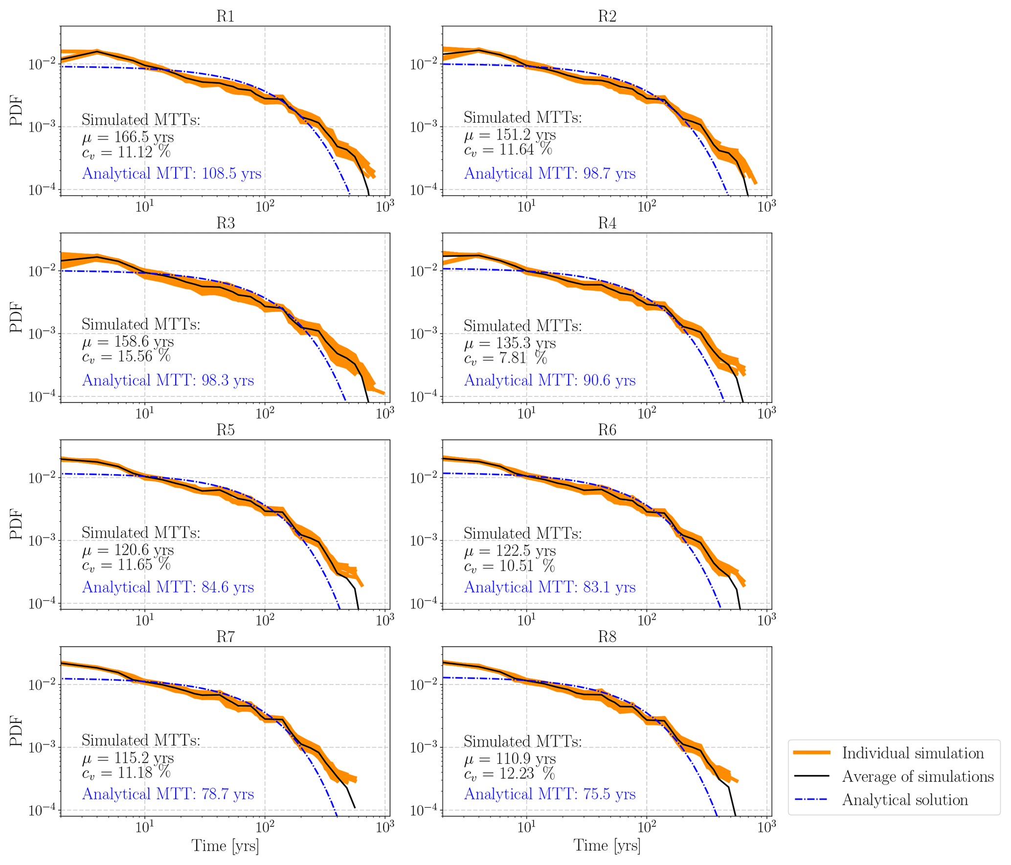
Figure 7Travel time distributions of ensemble simulations and analytical solutions categorized by recharge realization. The orange lines show the simulated TTDs of all realizations of Ks fields for each recharge realization. The black lines denote the ensemble-averaged TTDs of each recharge realization. The blue dash-dot line is the fit analytical TTD under the RS assumption. The analytical MTT, the mean (μ), and the coefficient of variance (cv) of the simulated MTTs are also shown in this figure.
Table 2Effective groundwater storages related to the transport process for each recharge realization.
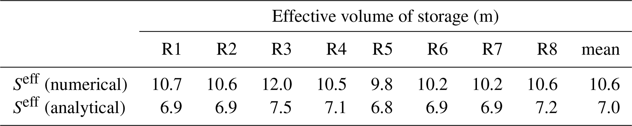
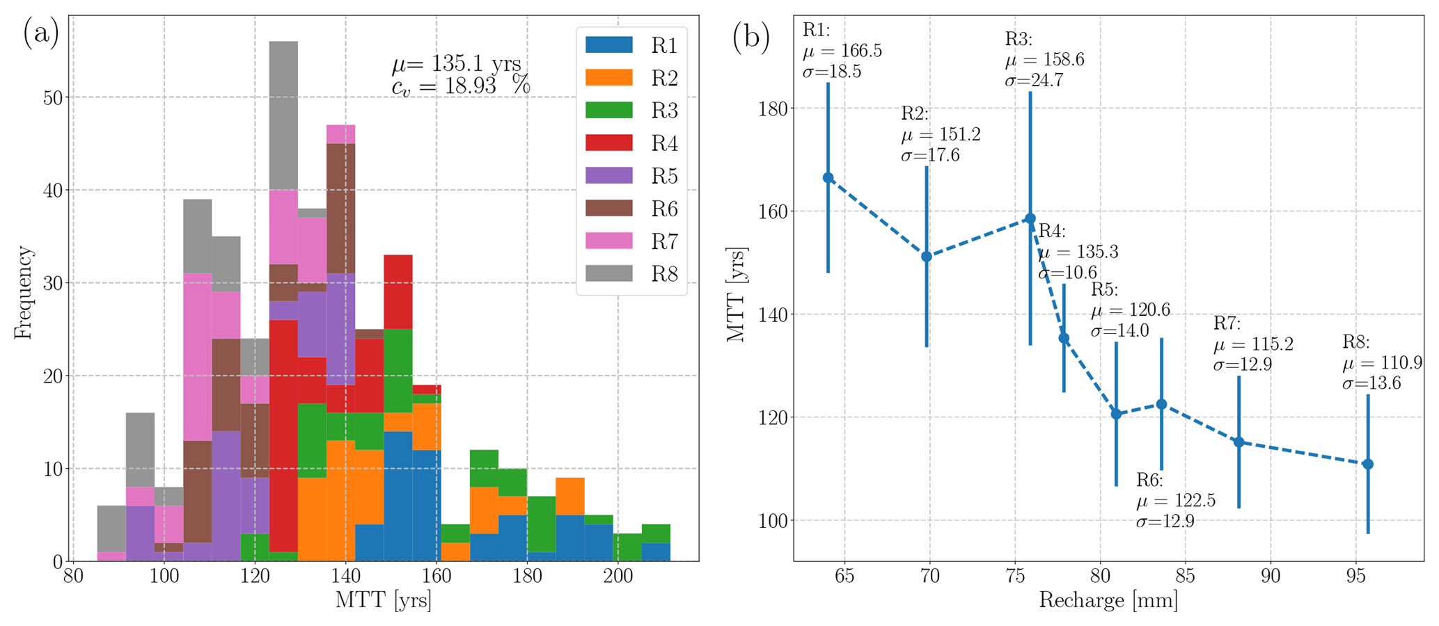
Figure 8Uncertainty quantification: Monte Carlo simulations of MTT predictions categorized by recharge realization. (a) shows a histogram of MTT predictions. (b) shows the relationship between the ensemble-averaged MTT (μ) and the spatially averaged recharge. The error bars represent the standard deviation of MTTs (σ) for each recharge realization.
4.2 Uncertainty of young/old water preference
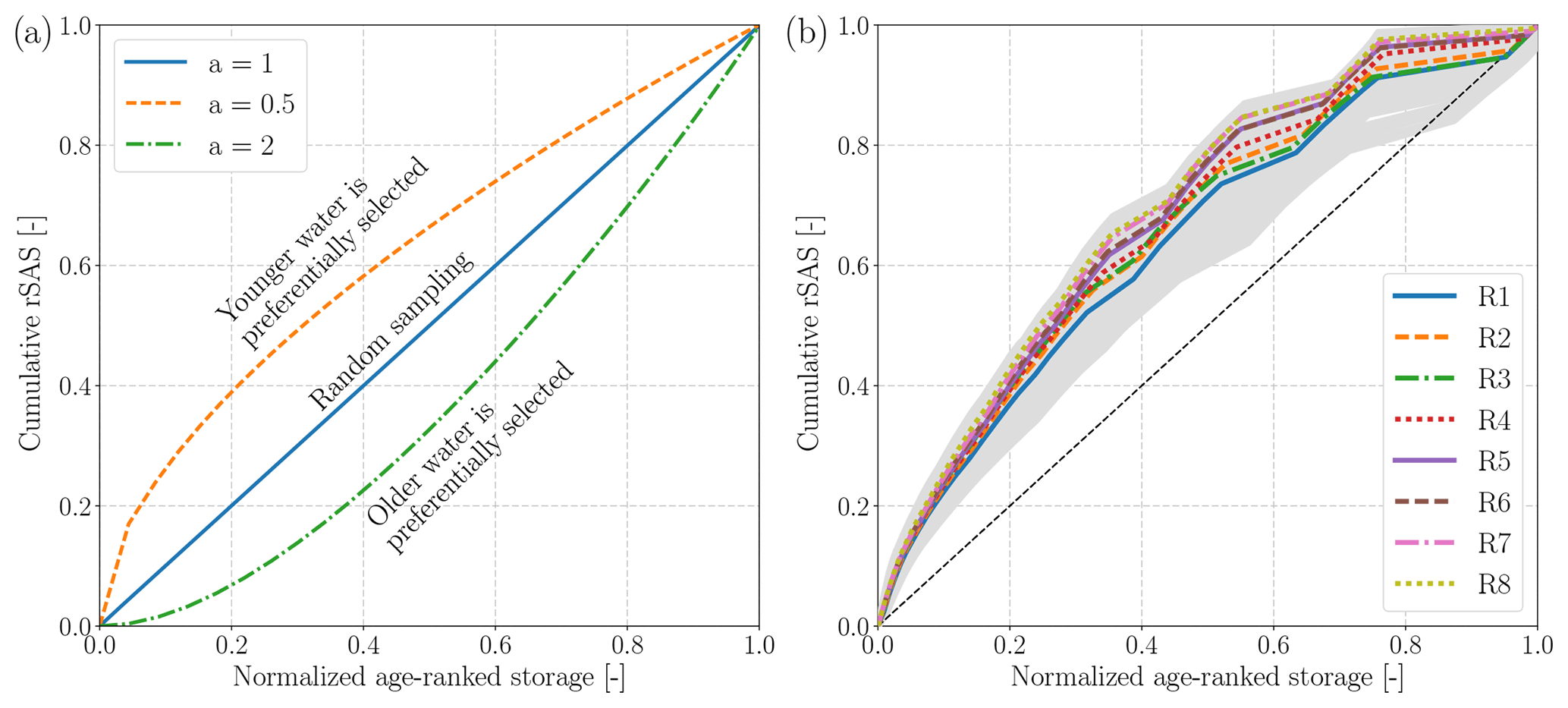
Figure 9Cumulative rank SAS functions as a function of normalized age-ranked storage. (a) Schematic of cumulative rank SAS functions parameterized by gamma distribution with the shape parameter a=0.5, 1, and 2. (b) Cumulative rank SAS functions of the ensemble simulations (light grey lines) and the ensemble average for each recharge realization.
Figure 9a provides an intuitive illustration of the relationship between the cumulative rank SAS functions and the systematic preference for discharging water with different ages. Figure 9b shows the cumulative rank SAS functions of all ensemble simulations (obtained from 400 realizations of Ks fields in eight recharge scenarios). The figure is categorized into eight groups by different colors and line styles, each representing a recharge realization. Generally, the system has a weak preference to select younger water as discharge, despite different recharge realizations and Ks realizations. Nevertheless, a moderate variation in SAS functions for the ensemble simulations can be observed. The variation of interest is introduced by the spatial distribution and velocity of flow pathlines that are controlled by different Ks fields. For example, a more permeable shallow aquifer layer will activate more flow pathways in this layer and thus will introduce a stronger preference for young water. In particular, the significant variation in hydraulic conductivities in the deepest geological layer (e.g., Lower Muschelkalk) has a pronounced impact on the discharge of old water. With a thickness of up to 100 m, the hydraulic conductivity of this layer controls how many water parcels can enter into this layer and how deep the flow paths can develop. This effect can be evidenced by a large difference in the SAS functions related to old ages and a relatively smaller difference in those related to young ages in Fig. 9b.
4.3 Sensitivity to the spatial pattern of recharge
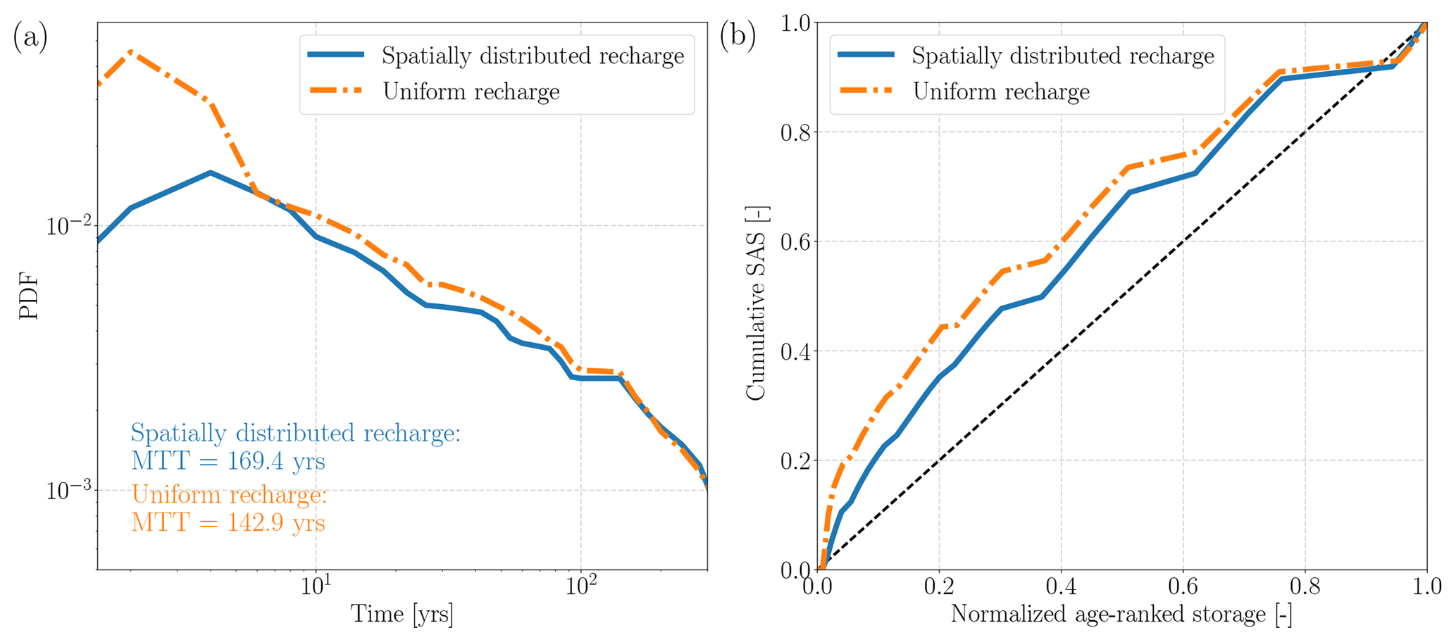
Figure 10Sensitivity of (a) TTDs and MTTs and (b) SAS functions to the spatial pattern of recharge.
Figure 10a depicts the sensitivity of simulated TTDs and MTTs to the spatial distribution of recharge, while Fig. 10b shows the sensitivity of the cumulative SAS function to the spatial pattern of recharge. The reference simulation is set up using the spatially uniform recharge that is equal to the spatial average of the spatially distributed recharge, while all of the other parameters in these two simulations are held identical. The different spatial distributions of recharge have a clear effect on the shape of TTDs. It appears that the most evident difference between the TTDs of the two recharge scenarios occurs at the early period. Additionally, the simulated MTT using the uniform recharge appears to be smaller than that using the spatially distributed recharge. Figure 10b indicates that the simulation using uniform recharge has a consistently stronger preference for sampling young water than the simulation using spatially distributed recharge. Nevertheless, both scenarios show a general preference for young water.
The difference in TTDs and SAS functions is not induced by the variability in internal hydraulic properties, since the two simulations share the same Ks field. Rather, it is mainly induced by the different flow paths of particle tracers in the two recharge scenarios. The spatially distributed recharge simulated by mHM reveals that the upstream mountainous area has higher recharge rates than those in the lowland plain. By contrast, the uniform recharge scenario neglects this spatial nonuniformity. This difference results in the following: (a) under a uniform recharge scenario, more particle tracers enter the system from locations near the streams at lowland plains (Fig. 3b), indicating that more particle tracers are transported in the local flow system rather than in the regional flow system (Toth, 1963); and (b) higher recharge rates at lowland plains accelerate the particles' movement in this area and shorten their travel times. As such, local particle flow paths within the shallow aquifer layer at lowland plains are activated, leading to a stronger preference for sampling local flow paths in shallow aquifer layers and therefore a stronger preference for young ages. Our findings are in line with the observations by Kaandorp et al. (2018), wherein the authors found a relatively higher preference for the selection of older water in the upstream area than that in the downstream area of the Springendalse Beek catchment.
5.1 Uncertainty of external forcing, internal property, and TTD predictions
In the idealized aquifers where groundwater flow is of the Dupuit–Forchheimer type, the recharge is uniform and the aquifer is locally homogeneous. TTD is controlled by recharge, saturated aquifer thickness, and porosity, and it is independent of hydraulic conductivity (Haitjema, 1995). In a real-world catchment with complex geometry and topography, stratigraphic aquifers, and nonuniform recharge, our numerical exploration demonstrates that the groundwater TTD is dependent on both recharge and the hydrostratigraphic Ks field.
The mechanisms behind the effects of the recharge rate and the Ks field are different. Given that the spatial pattern of recharge remains the same, a higher recharge rate intensifies the fluxes for the complete range of flow pathways. This process forces water downward in the recharge zones and upward to the discharge area. As such, flow rates through all flow pathways are increased equally, and the spatial distribution of flow pathways is not changed. The corresponding SAS function is also not changed (Botter et al., 2010; Cartwright and Morgenstern, 2015; Kaandorp et al., 2018). In contrast, a different Ks field activates flow pathways in more permeable layers, deactivates flow pathways in less permeable layers, changes the spatial distribution of flow pathways, and therefore changes the shape of the SAS function (Harman et al., 2016; Kim et al., 2016).
We also underline the value of observational data in reducing predictive uncertainty in simulated TTDs. In this study, the majority of model parameters can be adequately conditioned by spatially distributed groundwater head observations (Fig. 4). Provided that most of the hydraulic conductivities are constrained to the model-to-measurement misfit and reality, the TTD predictions can also be effectively bounded. This is evidenced by Fig. 7, from which moderate values of cv ranging from 7.81 % to 15.56 % in different recharge realizations can be observed. The ensemble-averaged MTTs for different recharge realizations also have a high cv (15.70 %), implying that the TTD prediction appears highly sensitive to recharge. Our findings are in line with Danesh-Yazdi et al. (2018), in which the interplay between recharge and subsurface heterogeneity was investigated and a strong dependency of TTDs on the recharge was observed.
5.2 Analytical model and SAS functions
The analytical solution of TTD, assuming a random sampling of water, cannot properly replicate the TTD of numerical simulation in the study domain. In the stratigraphic aquifer with complex topography and diffuse recharge, the analytical solution using Eq. (6) underestimates the MTT. Note that this conclusion holds when the simulated TTD has a relatively larger long-tail behavior than the exponential distribution. Such observations have also been reported for other real-world aquifers (Basu et al., 2012; Eberts et al., 2012; Kaandorp et al., 2018). This finding can be seen as an extension of Basu et al. (2012), in which the authors found a moderate discrepancy between the analytical solution using Eq. (6) and the numerical solution in a small catchment.
It is obvious that the analytical solution under the RS assumption cannot explicitly include the impact of the distributed hydraulic properties of stratigraphic aquifers and the spatially nonuniform recharge. The above limitations of analytical models may introduce a significant predictive error for the TTD predictions, as shown in Fig. 7. Moreover, the effective volume of storage related to the transport process Seff is calculated utilizing the numerical solutions of distributed models. As a first-order approximation of effective storage volume, it suggests that only a small fraction of total groundwater volume is involved in the active hydrologic cycle.
The SAS function provides a good interpretability for simulation results using the fully distributed model in terms of characterizing the preference for releasing water of different ages. We find that the SAS functions are weakly dependent on the Ks fields in the stratigraphic aquifer system, but the overall preference for young water does not change. This weak dependency can be explained by the fact that different realizations of Ks fields modify the spatial distribution of particle flow paths. The overall tendency for young groundwater in the saturated aquifer has been reported by many past studies (Danesh-Yazdi et al., 2018; Kaandorp et al., 2018; Yang et al., 2018). Our study links the explicit simulations of travel times and the analytical SAS functions and offers original insights into the uncertainty propagated from recharge and the Ks fields to the SAS functions.
5.3 Dependency of TTDs and SAS functions on the spatial pattern of forcings
The sensitivity of the TTDs and SAS functions to the spatial pattern of recharge forcings can be explained mainly by the different flow paths of particle tracers, resulting primarily from the spatially heterogeneous fields of recharge across the study catchment. For the regional groundwater system, the spatial variation of recharge determines the distribution of starting points of the flow pathlines of tracer particles. For example, more particles will be injected from recharge zones that are typically located in high-elevation regions, resulting in a higher weight of flowlines starting from high-elevation regions. The pronounced spatial variability of recharge also controls the systematic (water age) preference for particles existing from the system (to river discharge) that originated from different regions and therefore exerts a strong control on the shape of the SAS function.
In the study catchment, an oversimplified spatially uniform recharge results in a smaller MTT and a stronger preference for discharging young water compared to those taking the spatial variability of recharge. Such observations are conditioned to site-specific features of the study catchment, which is noticed only when the following apply: (a) a site is located in a headwater catchment under a humid climate condition; (b) the recharge rate in areas close to the drainage network is generally lower than that in areas far away from the drainage network; and (c) the system is under (near) natural conditions, meaning that artificial drainage and pumping do not dominate the groundwater budget.
The assumption of spatially uniform input forcing has been widely applied in regional-scale subsurface hydrologic models (Yang et al., 2018; Zghibi et al., 2015). Our study indicates that a reasonable characterization of spatial patterns of recharge is crucial for reliable TTD prediction. Unfortunately, it is quite challenging to confidently quantify the groundwater recharge at the regional scale under today's technique due to the lack of reliable measurements (Cheng et al., 2017; Healy and Scanlon, 2010; Zink et al., 2017). Appropriate techniques should be chosen to estimate groundwater recharge according to the study goals and the spatial and temporal scales.
5.4 Implications for the applied groundwater modeling
Uncertainty limits the applicability of groundwater models. Most of the applied groundwater models are deterministic models that use direct values of inputs and parameters instead of probabilistic distributions of them. Specifically, both the model inputs and the inversion process are deterministic, leading to a deterministic best-fit parameter set achieved during model calibration. Our study reveals limitations of the above modeling procedure and suggests that the probabilistic distribution of inputs and parameters should be considered for the applied modeling. The main limitation is that the single exclusive assignment of recharge is inadequate for the simulation of transport processes because the error can be propagated from inputs to the conditioned parameters (e.g., hydraulic conductivities) through the calibration process (Fig. 4). This accumulated error will further lead to a seriously biased prediction of travel times. Additionally, the modeling workflow used in this study is computationally more efficient than the Bayesian approach and is suitable for complex real-world applications.
The degree of predictive uncertainty is highly dependent on the parameterization scheme. Some highly parameterized models are potentially ill posed due to the paucity of data and therefore cannot be constrained by the available calibration dataset. In this case, the predictive uncertainty of TTDs is potentially high (Danesh-Yazdi et al., 2018; Weissmann et al., 2002). Stratigraphic aquifer models with zoned parameters are still widely used for applied groundwater modeling because the field representation of local-scale heterogeneity is difficult. Given that the aquifer model is stratigraphic and the number of parameters is less than the number of observations, most of the adjustable parameters can be effectively bounded. In this case, the uncertainty of input data (e.g., recharge) appears to have a primary influence on the TTD predictions. Note that here we do not account for the error caused by model structural deficiency.
In this study, we explore the relationship between the uncertainty of recharge, calibration-constrained hydraulic conductivity realizations, and predictions of groundwater TTDs. Using both a physically based numerical model and a lumped analytical model, a comprehensive case study is performed in an agricultural catchment (the Nägelstedt catchment). The RWPT method is used to track the water samples through the modeling domain and compute their travel times. Moreover, the analytical model is fit against the numerical solutions to provide a reference for the effective storage and sampling behavior of the system. Based on this study, the following conclusions are drawn.
-
In the Nägelstedt catchment model, the simulated MTTs are strongly dependent on the recharge rate and weakly dependent on the postcalibrated Ks field. We highlight the importance of recharge quantification and the worth of reliable data in reducing the predictive uncertainty of TTDs.
-
The framework of the SAS function provides a good interpretability of simulated TTDs in terms of characterizing the systematic preference for sampling young/old water as outflow. On the basis of this framework, we find that the ensemble simulations have a consistent preference for young water, despite the different recharge and hydraulic conductivity realizations. Our study provides a novel modeling framework to explore the effect of input uncertainty and parameter equifinality on TTDs and SAS functions through a combination of calibration-constrained Monte Carlo parameter generation, a numerical model, and a SAS function framework.
-
Both the shape and the breadth of catchment groundwater TTDs and SAS functions are sensitive to the spatial distribution of recharge. Therefore, a reasonable characterization of the spatial pattern of recharge is crucial for the reliable TTD prediction in the catchment-scale groundwater models.
The source code of the coupled model mHM-OGS v1.0 can be freely accessed via the following on-line repository: https://doi.org/10.5281/zenodo.1248005 (Jing et al., 2018b).
Random walk particle tracking solves a diffusion equation at local Lagrangian coordinates rather than the classical advection–diffusion equation, which can be expressed as
where x denotes the coordinates of the particle location, Δt denotes the time step size, and Z denotes a Gaussian random number, with the mean being zero and the variance being unity.
The velocity v in Eq. (A1) is replaced by to maintain consistency with the classical advection–dispersion equation (Kinzelbach, 1986). The expressions of and the hydrodynamic dispersion tensor Dij are
where δij denotes the Kronecker symbol, αL denotes the longitudinal dispersion length, αT denotes the transverse dispersion length, denotes the tensor of the molecular diffusion coefficient, and vi denotes the mean pore velocity component in the ith direction.
The stochastic governing equation of 3-D RWPT can therefore be expressed as
where x, y, and z are the spatial coordinates of a particle, Δt is the time step, and Zi is a random number with a mean of zero and a unit variance.
Table B1Composite parameter sensitivities to the groundwater head observations.
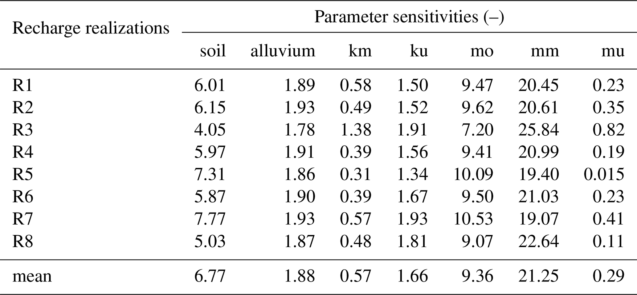
The PEST algorithm calculates the sensitivity with respect to each parameter of all observations (with the latter weighted as per user-assigned weights), namely the “composite sensitivity” (Doherty, 2015). The composite sensitivity of parameter i is defined as , where J denotes the Jacobian matrix that includes the sensitivities of all predictions to all model parameters, Q is the weight matrix, and n is the number of observations with nonzero weights. In this study, all weights assigned to observations are equally set to 1. Table B1 displays the composite parameter sensitivities in each recharge realization. The mean composite parameter sensitivities of calibrations in all recharge realizations are also included in this table. The hydraulic conductivity of the Middle Muschelkalk (mm) is highly sensitive to groundwater head observations, whereas that of the Lower Muschelkalk (mu) is insensitive to groundwater head observations. The sensitivity of mu, however, varies widely between different recharge realizations, from the highest one in R3 (0.82) to the lowest one in R5 (0.015).
The authors declare that they have no conflict of interest.
This study receives support from the Deutsche Forschungsgemeinschaft via
Sonderforschungsbereich CRC 1076 AquaDiva. We kindly thank Sabine Sattler
from the Thuringian State office for the Environment and Geology (TLUG) for
providing basic geological data. We acknowledge the EVE Linux Cluster team at
UFZ for their support for this study. We also acknowledge the Chinese
Scholarship Council (CSC) for supporting Miao Jing's stay in
Germany.
The article processing charges for
this open-access
publication were covered by a Research
Centre of the Helmholtz Association.
Edited by: Brian Berkowitz
Reviewed by: Erwin
Zehe and one anonymous referee
Aigner, T.: Calcareous Tempestites: Storm-dominated Stratification in Upper Muschelkalk Limestones (Middle Trias, SW-Germany), in: Cyclic and Event Stratification, edited by: Einsele, G. and Seilacher, A., 180–198, Springer Berlin Heidelberg, Berlin, Heidelberg, 1982. a
Ajami, N. K., Duan, Q., and Sorooshian, S.: An integrated hydrologic Bayesian multimodel combination framework: Confronting input, parameter, and model structural uncertainty in hydrologic prediction, Water Resour. Res., 43, W01403, https://doi.org/10.1029/2005WR004745, 2007. a
Basu, N. B., Jindal, P., Schilling, K. E., Wolter, C. F., and Takle, E. S.: Evaluation of analytical and numerical approaches for the estimation of groundwater travel time distribution, J. Hydrol., 475, 65–73, https://doi.org/10.1016/j.jhydrol.2012.08.052, 2012. a, b, c
Benettin, P., Kirchner, J. W., Rinaldo, A., and Botter, G.: Modeling chloride transport using travel time distributions at Plynlimon, Wales, Water Resour. Res., 51, 3259–3276, https://doi.org/10.1002/2014WR016600, 2015. a, b, c
Benettin, P., Soulsby, C., Birkel, C., Tetzlaff, D., Botter, G., and Rinaldo, A.: Using SAS functions and high-resolution isotope data to unravel travel time distributions in headwater catchments, Water Resour. Res., 53, 1864–1878, https://doi.org/10.1002/2016WR020117, 2017. a
Benson, D. A., Aquino, T., Bolster, D., Engdahl, N., Henri, C. V., and Fernandez-Garcia, D.: A comparison of Eulerian and Lagrangian transport and non-linear reaction algorithms, Adv. Water Resour., 99, 15–37, https://doi.org/10.1016/j.advwatres.2016.11.003, 2017. a
Beven, K.: Prophecy, reality and uncertainty in distributed hydrological modelling, Adv. Water Resour., 16, 41–51, 1993. a
Böhlke, J. K.: Groundwater recharge and agricultural contamination, Hydrogeol. J., 10, 153–179, https://doi.org/10.1007/s10040-001-0183-3, 2002. a
Botter, G., Bertuzzo, E., and Rinaldo, A.: Transport in the hydrologic response: Travel time distributions, soil moisture dynamics, and the old water paradox, Water Resour. Res., 46, 1–18, https://doi.org/10.1029/2009WR008371, 2010. a
Botter, G., Bertuzzo, E., and Rinaldo, A.: Catchment residence and travel time distributions: The master equation, Geophys. Res. Lett., 38, 1–6, https://doi.org/10.1029/2011GL047666, 2011. a, b
Böhlke, J. K. and Denver, J. M.: Combined Use of Groundwater Dating, Chemical, and Isotopic Analyses to Resolve the History and Fate of Nitrate Contamination in Two Agricultural Watersheds, Atlantic Coastal Plain, Maryland, Water Resour. Res., 31, 2319–2339, https://doi.org/10.1029/95WR01584, 1995. a
Cartwright, I. and Morgenstern, U.: Transit times from rainfall to baseflow in headwater catchments estimated using tritium: the Ovens River, Australia, Hydrol. Earth Syst. Sci., 19, 3771–3785, https://doi.org/10.5194/hess-19-3771-2015, 2015. a, b
Cheng, Y., Zhan, H., Yang, W., Dang, H., and Li, W.: Is annual recharge coefficient a valid concept in arid and semi-arid regions?, Hydrol. Earth Syst. Sci., 21, 5031–5042, https://doi.org/10.5194/hess-21-5031-2017, 2017. a, b
Danesh-Yazdi, M., Klaus, J., Condon, L. E., and Maxwell, R. M.: Bridging the gap between numerical solutions of travel time distributions and analytical storage selection functions, Hydrol. Process., 32, 1063–1076, https://doi.org/10.1002/hyp.11481, 2018. a, b, c, d, e, f
de Rooij, R., Graham, W., and Maxwell, R. M.: A particle-tracking scheme for simulating pathlines in coupled surface-subsurface flows, Adv. Water Resour., 52, 7–18, https://doi.org/10.1016/j.advwatres.2012.07.022, 2013. a
Doherty, J.: Calibration and uncertainty analysis for complex environmental models, Watermark Numerical Computing, Brisbane, Australia, 2015. a, b, c, d, e, f
Doherty, J. and Hunt, R.: Approaches to highly parameterized inversion: a guide to using PEST for groundwater-model calibration, U. S. Geological Survey Scientific Investigations Report 2010-5169, p. 70, http://pubs.usgs.gov/sir/2010/5169/, 2010. a
Eberts, S. M., Böhlke, J. K., Kauffman, L. J., and Jurgens, B. C.: Comparison of particle-tracking and lumped-parameter age-distribution models for evaluating vulnerability of production wells to contamination, Hydrogeol. J., 20, 263–282, https://doi.org/10.1007/s10040-011-0810-6, 2012. a, b
Engdahl, N. B., McCallum, J. L., and Massoudieh, A.: Transient age distributions in subsurface hydrologic systems, J. Hydrol., 543, 88–100, https://doi.org/10.1016/j.jhydrol.2016.04.066, 2016. a, b, c
Fischer, T., Naumov, D., Sattler, S., Kolditz, O., and Walther, M.: GO2OGS 1.0: a versatile workflow to integrate complex geological information with fault data into numerical simulation models, Geosci. Model Dev., 8, 3681–3694, https://doi.org/10.5194/gmd-8-3681-2015, 2015. a
Ginn, T. R.: On the distribution of multicomponent mixtures over generalized exposure time in subsurface flow and reactive transport: Theory and formulations for residence-time-dependent sorption/desorption with memory, Water Resour. Res., 36, 2885–2893, https://doi.org/10.1029/2000WR900170, 2000. a
Goode, D. J.: Direct simulation of groundwater age, Water Resour. Res., 32, 289–296, https://doi.org/10.1029/95WR03401, 1996. a
Haitjema, H.: On the residence time distribution in idealized groundwater sheds, J. Hydrol., 172, 127–146, 1995. a, b, c, d, e, f
Hale, V. C. and McDonnell, J. J.: Effect of bedrock permeability on stream base flow mean transit time scaling relations: 1. A multiscale catchment intercomparison, Water Resour. Res., 52, 1358–1374, 2016. a
Harman, C. J.: Time-variable transit time distributions and transport: Theory and application to storage-dependent transport of chloride in a watershed, Water Resour. Res., 51, 1–30, 2015. a, b, c, d
Harman, C. J., Ward, A. S., and Ball, A.: How does reach-scale stream-hyporheic transport vary with discharge? Insights from rSAS analysis of sequential tracer injections in a headwater mountain stream, Water Resour. Res., 52, 7130–7150, https://doi.org/10.1002/2016WR018832, 2016. a
Healy, R. W. and Scanlon, B. R.: Estimating Groundwater Recharge, Cambridge University Press, https://doi.org/10.1017/CBO9780511780745, 2010. a, b
Heße, F., Zink, M., Kumar, R., Samaniego, L., and Attinger, S.: Spatially distributed characterization of soil-moisture dynamics using travel-time distributions, Hydrol. Earth Syst. Sci., 21, 549–570, https://doi.org/10.5194/hess-21-549-2017, 2017. a, b, c, d
Howden, N. J. K., Burt, T. P., Worrall, F., Whelan, M. J., and Bieroza, M.: Nitrate concentrations and fluxes in the River Thames over 140 years (1868–2008): are increases irreversible?, Hydrol. Process., 24, 2657–2662, https://doi.org/10.1002/hyp.7835, 2010. a
Jing, M., Heße, F., Kumar, R., Wang, W., Fischer, T., Walther, M., Zink, M., Zech, A., Samaniego, L., Kolditz, O., and Attinger, S.: Improved regional-scale groundwater representation by the coupling of the mesoscale Hydrologic Model (mHM v5.7) to the groundwater model OpenGeoSys (OGS), Geosci. Model Dev., 11, 1989–2007, https://doi.org/10.5194/gmd-11-1989-2018, 2018a. a, b, c, d, e
Jing, M., Heße, F., Kumar, R., Wang, W., Fischer, T., Walther, M., Zink, M., Zech, A., Samaniego, L., Kolditz, O., and Attinger, S.: mHM#OGS v1.0: the coupling interface between the mesoscale Hydrologic Model (mHM) and the groundwater model OpenGeoSys (OGS) (Version 1.0), Zenodo, https://doi.org/10.5281/zenodo.1248005, 16 May 2018b.
Jochen, L., Lepper, J., Rambow, D., and Röhling, H. G.: Lithostratigraphie des Buntsandstein in Deutschland, Schriftenreihe der Deutschen Gesellschaft für Geowissenschaften, 69, 69–149, 2014. a, b
Kaandorp, V. P., de Louw, P. G. B., van der Velde, Y., and Broers, H. P.: Transient Groundwater Travel Time Distributions and Age-Ranked Storage-Discharge Relationships of Three Lowland Catchments, Water Resour. Res., 54, 1–18, https://doi.org/10.1029/2017WR022461, 2018. a, b, c, d, e
Kim, M., Pangle, L. A., Cardoso, C., Lora, M., Volkmann, T. H. M., Wang, Y., Harman, C. J., and Troch, P. A.: Transit time distributions and StorAge Selection functions in a sloping soil lysimeter with time-varying flow paths: Direct observation of internal and external transport variability, Water Resour. Res., 52, 7105–7129, https://doi.org/10.1002/2016WR018620, 2016. a
Kinzelbach, W.: Groundwater modelling: an introduction with sample programs in BASIC, vol. 25, Elsevier, 1986. a
Kirchner, J. W.: Aggregation in environmental systems – Part 1: Seasonal tracer cycles quantify young water fractions, but not mean transit times, in spatially heterogeneous catchments, Hydrol. Earth Syst. Sci., 20, 279–297, https://doi.org/10.5194/hess-20-279-2016, 2016. a
Kohlhepp, B., Lehmann, R., Seeber, P., Küsel, K., Trumbore, S. E., and Totsche, K. U.: Aquifer configuration and geostructural links control the groundwater quality in thin-bedded carbonate–siliciclastic alternations of the Hainich CZE, central Germany, Hydrol. Earth Syst. Sci., 21, 6091–6116, https://doi.org/10.5194/hess-21-6091-2017, 2017. a, b, c, d
Kolditz, O., Bauer, S., Bilke, L., Böttcher, N., Delfs, J. O., Fischer, T., Görke, U. J., Kalbacher, T., Kosakowski, G., McDermott, C. I., Park, C. H., Radu, F., Rink, K., Shao, H., Shao, H. B., Sun, F., Sun, Y. Y., Singh, A. K., Taron, J., Walther, M., Wang, W., Watanabe, N., Wu, Y., Xie, M., Xu, W., and Zehner, B.: OpenGeoSys: an open-source initiative for numerical simulation of thermo-hydro-mechanical/chemical (THM/C) processes in porous media, Environ. Earth Sci., 67, 589–599, https://doi.org/10.1007/s12665-012-1546-x, 2012. a, b
Kumar, R., Samaniego, L., and Attinger, S.: Implications of distributed hydrologic model parameterization on water fluxes at multiple scales and locations, Water Resour. Res., 49, 360–379, https://doi.org/10.1029/2012WR012195, 2013. a
Leray, S., Engdahl, N. B., Massoudieh, A., Bresciani, E., and McCallum, J.: Residence time distributions for hydrologic systems: Mechanistic foundations and steady-state analytical solutions, J. Hydrol., 543, 67–87, https://doi.org/10.1016/j.jhydrol.2016.01.068, 2016. a, b, c, d
McCallum, J. L., Engdahl, N. B., Ginn, T. R., and Cook, P. G.: Nonparametric estimation of groundwater residence time distributions: What can environmental tracer data tell us about groundwater residence time?, Water Resour. Res., 50, 2022–2038, https://doi.org/10.1002/2013WR014974, 2014. a
McCann, T.: The Geology of Central Europe Volume 2: Mesozoic and Cenozoic, Geological Society of London, https://doi.org/10.1144/CEV2P, 2008. a
Menning, M.: Deutsche Stratigraphische Kommission (2002), Eine geologische Zeitskala 2002, edited by: Deutsche Stratigraphische Kommission, Stratigraphische Tabelle von Deutschland, 2002. a
Merz, G.: Zur Petrographie, Stratigraphie, Paläogeographie und Hydrogeologie des Muschelkalks (Trias) im Thüringer Becken, Zeitschrift der geologischen Wissenschaften, 15, 457–473, 1987. a
Molnat, J. and Gascuel-Odoux, C.: Modelling flow and nitrate transport in groundwater for the prediction of water travel times and of consequences of land use evolution on water quality, Hydrol. Process., 16, 479–492, https://doi.org/10.1002/hyp.328, 2002. a
Neuman, S. P.: Theory of flow in unconfined aquifers considering delayed response of the water table, Water Resour. Res., 8, 1031–1045, https://doi.org/10.1029/WR008i004p01031, 1972. a
Park, C. H., Beyer, C., Bauer, S., and Kolditz, O.: Using global node-based velocity in random walk particle tracking in variably saturated porous media: Application to contaminant leaching from road constructions, Environ. Geol., 55, 1755–1766, https://doi.org/10.1007/s00254-007-1126-7, 2008. a, b
Remondi, F., Kirchner, J. W., Burlando, P., and Fatichi, S.: Water Flux Tracking With a Distributed Hydrological Model to Quantify Controls on the Spatiotemporal Variability of Transit Time Distributions, Water Resour. Res., 54, 3081–3099, https://doi.org/10.1002/2017WR021689, 2018. a
Rinaldo, A., Beven, K. J., Bertuzzo, E., Nicotina, L., Davies, J., Fiori, A., Russo, D., and Botter, G.: Catchment travel time distributions and water flow in soils, Water Resour. Res., 47, 1–13, https://doi.org/10.1029/2011WR010478, 2011. a
Samaniego, L., Kumar, R., and Attinger, S.: Multiscale parameter regionalization of a grid-based hydrologic model at the mesoscale, Water Resour. Res., 46, W05523, https://doi.org/10.1029/2008WR007327, 2010. a
Schoups, G., van de Giesen, N. C., and Savenije, H. H. G.: Model complexity control for hydrologic prediction, Water Resour. Res., 44, W00B03, https://doi.org/10.1029/2008WR006836, 2008. a
Seidel, H. G. (Ed.): Geologie von Thüringen, Schweizerbart Science Publishers, Stuttgart, Germany, available at: http://www.schweizerbart.de//publications/detail/isbn/9783510652051/Geologie_von_Thuringen_herausg_v_G_Se (last access: 10 anuary 2019), 2003. a, b, c
Selle, B., Rink, K., and Kolditz, O.: Recharge and discharge controls on groundwater travel times and flow paths to production wells for the Ammer catchment in southwestern Germany, Environ. Earth Sci., 69, 443–452, https://doi.org/10.1007/s12665-013-2333-z, 2013. a
Stewart, M. K., Morgenstern, U., McDonnell, J. J., and Pfister, L.: The `hidden streamflow' challenge in catchment hydrology: a call to action for stream water transit time analysis, Hydrol. Process., 26, 2061–2066, 2012. a
Stewart, M. K., Morgenstern, U., Gusyev, M. A., and Maloszewski, P.: Aggregation effects on tritium-based mean transit times and young water fractions in spatially heterogeneous catchments and groundwater systems, Hydrol. Earth Syst. Sci., 21, 4615–4627, https://doi.org/10.5194/hess-21-4615-2017, 2017. a
Tetzlaff, D., Birkel, C., Dick, J., Geris, J., and Soulsby, C.: Storage dynamics in hydropedological units control hillslope connectivity, runoff generation, and the evolution of catchment transit time distributions, Water Resour. Res., 50, 969–985, https://doi.org/10.1002/2013WR014147, 2014. a
Tompson, A. F. and Gelhar, L. W.: Numerical simulation of solute transport in three-dimensional, randomly heterogeneous porous media, Water Resour. Res., 26, 2541–2562, 1990. a
Tonkin, M. and Doherty, J.: Calibration-constrained Monte Carlo analysis of highly parameterized models using subspace techniques, Water Resour. Res., 45, 1–17, https://doi.org/10.1029/2007WR006678, 2009. a
Toth, J.: A Theoretical Analysis of Groundwater Flow in Small Drainage Basins, J. Geophys. Res., 68, 4795–4812, https://doi.org/10.1029/JZ068i016p04795, 1963. a
Van Der Velde, Y., Torfs, P. J. J. F., Van Der Zee, S. E. A. T. M., and Uijlenhoet, R.: Quantifying catchment-scale mixing and its effect on time-varying travel time distributions, Water Resour. Res., 48, 1–13, https://doi.org/10.1029/2011WR011310, 2012. a, b
van der Velde, Y., Heidbüchel, I., Lyon, S. W., Nyberg, L., Rodhe, A., Bishop, K., and Troch, P. A.: Consequences of mixing assumptions for time-variable travel time distributions, Hydrol. Process., 29, 3460–3474, https://doi.org/10.1002/hyp.10372, 2015. a
Van Meter, K., Basu, N., Veenstra, J., and Burras, C. L.: The nitrogen legacy: emerging evidence of nitrogen accumulation in anthropogenic landscapes, Environ. Res. Lett., 11, 035014, https://doi.org/10.1088/1748-9326/11/3/035014, 2016. a
Van Meter, K. J., Basu, N. B., and Van Cappellen, P.: Two centuries of nitrogen dynamics: Legacy sources and sinks in the Mississippi and Susquehanna River Basins, Global Biogeochem. Cy., 31, 2–23, https://doi.org/10.1002/2016GB005498, 2017. a
Wang, H., Richardson, C. J., Ho, M., and Flanagan, N.: Drained coastal peatlands: A potential nitrogen source to marine ecosystems under prolonged drought and heavy storm events – A microcosm experiment, Sci. Total Environ., 566–567, 621–626, https://doi.org/10.1016/j.scitotenv.2016.04.211, 2016. a
Wechsung, F., Kaden, S., Behrendt, H., and Klöcking, B. (Eds.): Integrated Analysis of the Impacts of Global Change on Environment and Society in the Elbe Basin, Schweizerbart Science Publishers, Stuttgart, Germany, available at: http://www.schweizerbart.de//publications/detail/isbn/9783510 653041/Wechsung_Integrated_Analysis_of_the_Imp (last access: 10 January 2019), 2008. a, b, c, d, e
Weissmann, G. S., Zhang, Y., LaBolle, E. M., and Fogg, G. E.: Dispersion of groundwater age in an alluvial aquifer system, Water Resour. Res., 38, 16-1–16-13, https://doi.org/10.1029/2001WR000907, 2002. a
Yang, J., Heidbüchel, I., Musolff, A., Reinstorf, F., and Fleckenstein, J. H.: Exploring the Dynamics of Transit Times and Subsurface Mixing in a Small Agricultural Catchment, Water Resour. Res., 54, 2317–2335, https://doi.org/10.1002/2017WR021896, 2018. a, b, c
Zghibi, A., Zouhri, L., Chenini, I., Merzougui, A., and Tarhouni, J.: Modelling of the groundwater flow and of tracer movement in the porous and fissured media: chalk aquifer (Northern part of Paris Basin, France), Hydrol. Process., 30, 1916–1928, https://doi.org/10.1002/hyp.10746, 2015. a
Zink, M., Kumar, R., Cuntz, M., and Samaniego, L.: A high-resolution dataset of water fluxes and states for Germany accounting for parametric uncertainty, Hydrol. Earth Syst. Sci., 21, 1769–1790, https://doi.org/10.5194/hess-21-1769-2017, 2017. a, b, c, d