2.1 Model selection

The model was constructed using ParFlow, an integrated hydrologic modeling code, coupled to the Common Land Model (CLM), a land surface modeling code. The terminology “integrated hydrologic model” used here refers to the integration of variably saturated subsurface and overland flow processes and is not intended to imply that the model includes anthropogenic or biologic processes. ParFlow simulates saturated and unsaturated flow in three dimensions using Richards' equation, and relationships between pressure and relative saturation or permeability defined by the Van Genuchten pressure–saturation and pressure–relative-permeability relationships (Van Genuchten, 1980). Overland flow is modeled with the kinematic wave equation, with velocity found by Manning's equation. Energy and water balances at the surface are represented with CLM (Dai et al., 2003; Maxwell and Miller, 2005; Jefferson et al., 2017). CLM is coupled to ParFlow by passing the land surface water flux to ParFlow as a forcing in the top layer, and substituting ParFlow's computations for infiltration and streamflow routing within CLM (Maxwell and Miller, 2005).

ParFlow has a number of differences with commonly used models in other drought-related studies. It is instructive to compare ParFlow with the VIC model (Hamman et al., 2018; Liang et al., 1994) and the Soil Water Assessment Tool (SWAT, Neisch et al., 2011), not in order to criticize any model, but to illustrate the reasoning for model choice in this study. ParFlow allows any number of subsurface layers with any specified conductivity, and has vertical and lateral flow driven by pressure gradients. Soil moisture and groundwater are not distinguished; both are represented through pressure in a cell and solved for using Richards' equation. This three-dimensional variably saturated flow is the main difference between ParFlow and other models. While this detailed representation is an advantage for this study, it also leads to higher computational expense in ParFlow runs when compared to other models. VIC typically has three soil layers and does not simulate lateral flow between macroscale grid cells, although it includes a baseflow term for water leaving a cell to enter a stream. VIC is often applied to larger-scale modeling, while ParFlow can be used at any resolution. SWAT partitions groundwater into a “deep aquifer” which can have lateral flow to other subbasins and a “shallow aquifer” which contributes only to the stream. Soil moisture and groundwater are modeled separately. In contrast, ParFlow combines all of these processes at a variety of scales; in this model, scales are included from kilometer to subcontinental scale. (This does omit meter- and centimeter-scale processes such as biogeochemical cycles.) The detailed representation of subsurface processes makes ParFlow-CLM a suitable model to run numerical experiments whose results depend on physical processes and their interactions, as opposed to statistical fitting or simplified parameterizations.

2.2 Model configuration

The model domain covers the southern High Plains and Rocky Mountains, including portions of the Arkansas and Missouri river basins (Fig. 1) at a 1 km resolution. The domain is 1200 km by 1124 km and extends to a depth of 102 m, with five layers for a total of 6 744 000 computational cells. The lowest layer is 100 m thick and the other four layers are 1, 0.6, 0.3 and 0.1 m thick, listed from base to top. An overland-flow boundary condition, allowing free development of a stream network, was imposed at the top layer. A no-flow boundary condition was specified at the bottom and on all sides, with the exception of surface streams which can exit the domain. Due to computational expense, the runs in the present study were performed on the supercomputer Cori at the National Energy Research Scientific Computing Center (NERSC). In total, 1 year of the model required over 20 000 processor hours to calculate and this was completed in about a week of wall-clock time.

Figure 1The model domain (box) covers the southern High Plains of the US. Blue shading indicates the Missouri and Arkansas continental river basins.

Download

Inputs for the study were developed from the previous work of Maxwell and Condon (2016), who modeled hydrology across the continental US (CONUS). The basic input data and initial conditions follow Maxwell and Condon (2016). Inputs include slopes, soil types, vegetation, attributes of soils and geologic units, and initial pressure conditions (see Fig. 2). The slopes in the x (east–west) and y (north–south) directions were derived from a digital elevation model and sink-filled to ensure the entire domain was connected. The simulations presented here use the kinematic wave approximation of the overland flow equations and therefore require a domain with a connected drainage network, as slopes control surface flow routing. While natural depressions in the landscape exist, the literature suggests that it is difficult to distinguish these natural depressions and sinks from noise within the processed DEM (e.g., Kenny et al., 2008). Soil types were taken from the SSURGO database. Important soil attributes include porosity, permeability, specific storage and van Genuchten parameters, which control saturated and unsaturated flow. Initial subsurface pressure conditions were taken from the original CONUS run, to increase spinup efficiency. The vegetation dataset was taken from the USGS land cover trends dataset (Soulard et al., 2014). Important vegetative parameters include leaf and stem area index, roughness length and displacement heights, rooting distribution parameters, and reflectance and transmittance for leaves and stems (Maxwell and Condon, 2016). While most inputs were drawn from Condon and Maxwell (2016), the geologic layer of that study contained features that were geologically less realistic at the scale of the High Plains. The geology of the base layer was updated for this project using local data from the US Geological Survey (USGS, 1998, 2005).

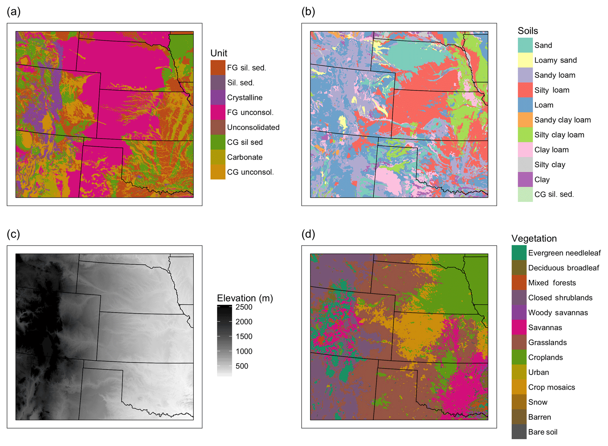
Figure 2Model inputs include (a) geology to characterize the bottom model layer, (b) soils to characterize upper layers, (c) topography for flow routing and (d) vegetation for surface energy and water exchanges.

Download

It is important to note that water management such as groundwater pumping, surface water storage and diversion, and irrigation are not included in these simulations. This means that results of the project represent the system in a pre-development state not including anthropogenic impacts to the hydrology (Maxwell and Condon, 2016). The only management impact represented was land use and its changes applied by setting and changing the land cover type in the model. The use of modern-day vegetation is not temporally consistent with preindustrial water management (Hurtt et al., 2011). However, in this project, we are not reconstructing any specific historical drought, so it is less important in addressing the research questions to match all forcings and settings to one period of time. Additionally, different crops may affect the details of drought evolution in different ways, but this is not represented here because ParFlow-CLM is not an agricultural model. Each cell is assigned one vegetation type and all crops are represented as the same “croplands” vegetation type. Analyzing the details of crop type and its impact is outside the scope of the present study and not critical to address the study questions.

The initial conditions for the simulation were obtained from the existing continental-scale simulations (Maxwell and Condon, 2016) and include 4 additional years of spinup prior to this project. The pressure file was subset to the High Plains domain and the geologic layer was updated as described in the Appendix. The model was run repeatedly with water year 1984 North American Land Data Assimilation System (NLDAS-2) forcing until average subsurface storage change in 1 year was less than 1 % of precipitation (achieved after three repeated runs). Ajami et al. (2014) showed that change in subsurface storage is one of the most rigorous spinup metrics for integrated hydrologic modeling. Holding this value below 1 % of precipitation means that effects seen in numerical experiments can be interpreted as meaningful, i.e., something besides spinup noise if they exceed the threshold.

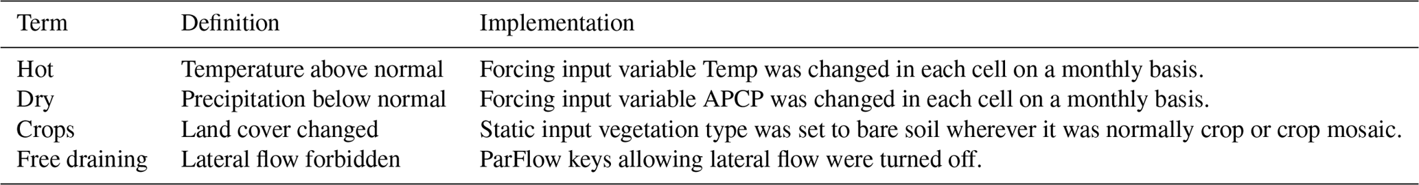
Table 1Numerical experiments were implemented through changes to the model temperature, precipitation, vegetative cover and internal settings.

Download Print Version | Download XLSX

2.3 Numerical experiments

A suite of synthetic drought scenarios were developed to explore the importance of precipitation, temperature and land cover change on regional drought response in the High Plains. All simulations are developed using the hourly observed NLDAS-2 historical atmospheric forcings from Water Year 1984 as a baseline (precipitation, temperature, pressure, humidity, short wave radiation, long wave radiation, wind speed). The experiments are outlined in Tables 1 and 2 and include a baseline run, three one-perturbation experiments exploring the effect of precipitation, temperature and land cover changes in isolation, a combined experiment with both temperature and precipitation changes, and a worst-case scenario which also includes land cover changes.

Table 2Model scenarios including run name and perturbations applied relative to the baseline scenario.

Download Print Version | Download XLSX

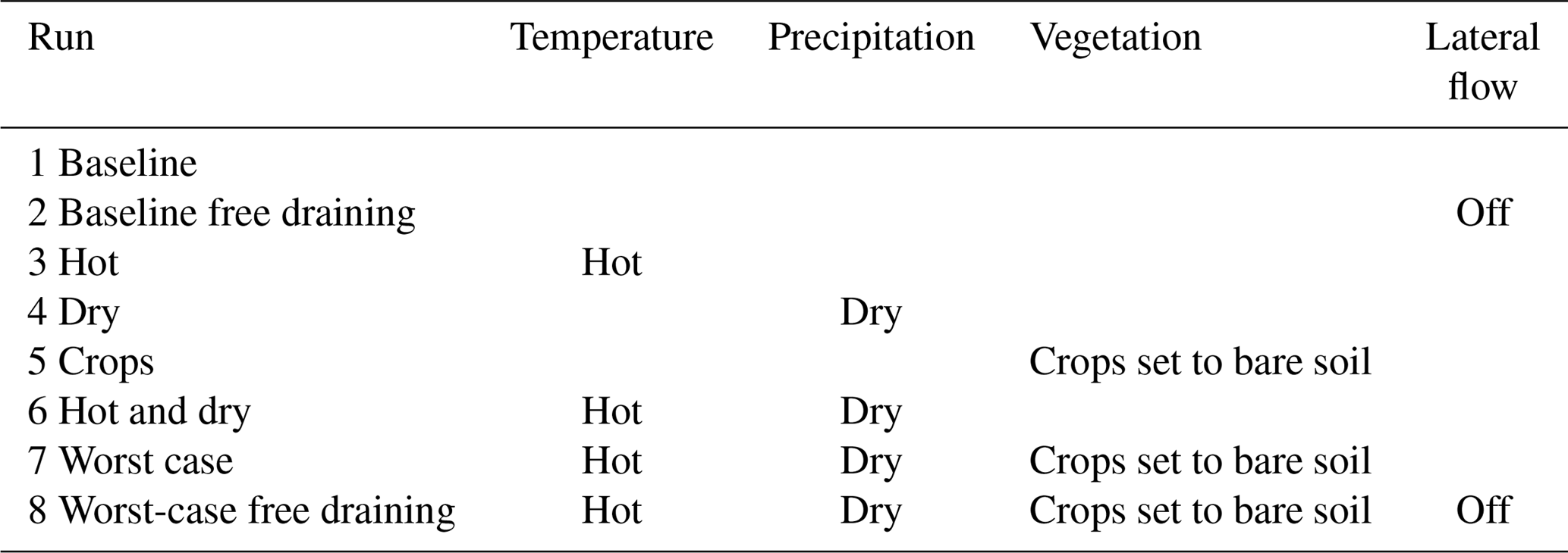
Two further runs were also conducted to explore the importance of lateral flow as a mechanism within the model as part of addressing the third research question on spatial scaling and complexity. Commonly used models including VIC and SWAT do not allow lateral flow within the model, and including this process makes the model computationally more expensive. Creating normal runs with lateral flow and free-draining runs (i.e., without lateral flow) allows exploration of how this process affects model results. To construct a free-draining run, the water table was set at the base of the domain and all overland and subsurface lateral flow processes were turned off, while vertical flow through the soil column and water table remained. (No separate spinup was conducted for the free-draining run, which has a lower water table than the other runs. To account for this, the free-draining drought run was compared to a free-draining baseline.) With these settings, ParFlow-CLM mimics a traditional land surface model as described in Maxwell and Condon (2016).

Definitions and specific implementation of each numerical experiment are shown in Table 2, and the exact perturbations used are quantified in Fig. 3. The baseline run and both free-draining runs were conducted for 1 year; the drought runs were conducted for 3 years of repeated drought forcing to simulate a transient time period a few years into a hypothetical severe drought. Although the simulation included 3 years, the analysis focuses on annually averaged results in the third and last year of model simulations in order to emphasize spatial scaling and factor interactions. Temporal evolution of drought is a large topic in itself and, while interesting, falls outside the scope of the present study.

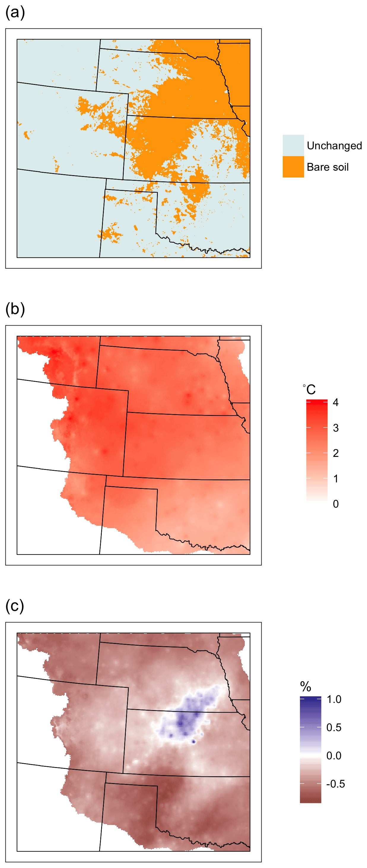
Figure 3Maps of the annual drought perturbations applied to the baseline scenario including (a) changes from cropland to bare soil, (b) absolute temperature increases and (c) relative precipitation increases.

Download

These experiments are synthetic drought scenarios that are not an exact reconstruction of any historical drought, but rather an example of severe meteorological drought based on the Dustbowl drought of the 1930s. They begin with a baseline water year, then add perturbations singly and in combination, as shown in Table 1. We used NLDAS forcing from Water Year 1984 as the baseline because it is one of the most average water years in the United States in recent decades. We then increased temperature and decreased precipitation using examples drawn from a major drought in the region. Temperature and precipitation perturbations of the NLDAS forcing are based on PRISM reconstructions of the Dustbowl drought (the most extreme drought in the modern historical record) (PRISM Climate Group, 2017). Since PRISM data have a coarser resolution than the model grid, the PRISM rasters were resampled to the model grid before preparing forcing data.

Perturbations were applied at monthly timescale for each cell of the domain. To find these meteorological drought changes, a spatial map of changes was prepared for each month of water year 1934, one of the worst drought years historically recorded in the region, relative to the baseline decade of 1920–1929. Months of water year 1934 were taken to represent a “drought January”, “drought February” etc. Months of the 1920s were averaged to arrive at a baseline for that region at that time, a “non-drought January”, “non-drought February” etc. Then these months were subtracted to create anomalies. For example, “non-drought January” temperature was subtracted from “drought January” temperature to find the January temperature anomaly. The averaging and subtraction was done for each grid cell of the model grid, producing a spatial map for each month.

Lastly, these spatial maps were used to perturb the baseline and produce forcings for drought runs. Temperature was perturbed by adding an absolute temperature change to each cell of the hourly forcing for the relevant month. Precipitation was perturbed by multiplying each cell of the hourly forcing by a relative change for the appropriate month. Lastly, vegetation was disturbed for the crops runs by setting all crop or crop mosaic cells to bare soil (this approximation was inspired by the documented massive crop failure during the historic Dustbowl). Figure 3 shows plots of the resulting annual anomalies in temperature, precipitation and land cover which were used to drive the perturbed simulations.

In real droughts, we know that drought perturbations will not occur in isolation. For instance, changing temperature would generally accompany changes in radiation, humidity, etc. Additionally the vegetative changes could be more complex, as shifting temperature and rainfall patterns can produce a range of responses across several vegetative types. Finally, real droughts could exceed the ranges of drought simulated within the study (for example, if temperature was increased far enough, it could have a larger impact than a small precipitation change). However, in our simulations we are isolating the primary driving factors to perturb the model and we do not include such secondary effects. This is an approximation, but the forcing is still suitable to address the research questions in this paper because the goal is not to simulate a projected climate change (with, for example, a Global Climate Model prediction) nor to predict an actual hydrologic drought.

By making a single change at a time, the analysis can attribute any differences between the baseline and the perturbed run to the single variable that was perturbed. This is an advantage of modeling studies over real world observations, as we can assess process interaction with much greater precision and detail. Changing humidity and pressure with associated temperature changes would be modifying three things at once, which limit the linearity arguments and the strength of the experiment as such. For example, Maxwell and Kollet (2008) perturbed temperature without changing other meteorological variables for a study of drought in the Little Washita watershed. Rasmussen et al. (2011) also employed a simplified approach they called “pseudo-global warming”, adding estimated climate perturbations in temperature, vapor mixing ratio, boundary layer height and wind speed to a forcing dataset. Markovich et al. (2016) perturbed temperature alone in a similar study of climate change in California, and Pribulick et al. (2016) perturbed temperature and land cover in studying the impacts of vegetation change under global warming in a Colorado watershed. While changing one meteorological variable does not fully represent the physical system, it is a documented simplification used in multiple published papers. This study uses single-factor perturbations to the model (forcing, land cover) in a systematic way to better quantify system sensitivity and evaluate how watershed response varies between driving factors.

2.4 Metrics of drought analysis

Several metrics are applied to quantify drought impacts. First, standard anomalies were calculated for all drought scenarios relative to the baseline by simply subtracting the baseline values. The term anomaly is used in this discussion to describe changes to hydrologic processes resulting from the perturbations applied to the simulations. The subtraction produces a simple metric of the model impact. Averaging the anomaly across the domain produced a measure of the total impact of a given factor. The single-perturbation model runs allowed the calculation of average impacts (I) for each factor alone: I (temperature), I (precipitation) and I (land cover). The multiperturbation runs allowed calculation of the impacts for the combined factors: I(temperature + precipitation + land cover) and I(temperature + precipitation).

We acknowledge that these calculated anomalies are not equivalent to published drought metrics that are often used to define hydrologic drought. These calculations were chosen for this analysis in order to specifically evaluate the research questions being addressed, through specific focus on hydrological variables such as soil moisture, water table level, runoff and ET.

The individual run impacts make it possible to assess whether impacts were linearly additive. If impacts are linearly additive, then the impacts of multiperturbation runs (e.g., I(temperature + precipitation)) should equal the sum of the composite individual perturbation runs (e.g., I(temperature) + I(precipitation)). Here we quantify the nonlinearity in the combined drought response as a percent difference between the multiperturbation impact and the expected impact assuming linear addition.

In analyzing model results, it is important to note that these results do not constitute a direct prediction or reconstruction of a specific historical drought, therefore we do not directly validate the simulated drought impacts against observations. Comparison to data is an important and challenging step of model studies. There are observations that could be used to explore the same research questions that are addressed here; however, none of them are directly comparable to the present model because the present model is not a reconstruction of any historical drought. The findings of this model, therefore, cannot be taken as a direct prediction for central North America. Rather, their value lies in suggesting system-scale phenomena such as the nonlinear combination of factors.

3.1 Description of simulated drought impacts

This section characterizes hydrologic drought impacts produced by the meteorological drought simulated in the hot and dry runs. Here we focus on ET and soil moisture impacts and put the simulated anomalies in the context of seasonal and spatial variability. The next section takes a broader approach to compare more runs and more variables, with less intensive detail.

Figure 4 shows that drought impacts on ET are relatively small compared to annual changes, but impacts to soil moisture are on the order of annual fluctuations. In the baseline year, ET is low in the fall, winter and early spring but becomes large in May–September, fluctuating between approximately 10 and 80 mm month⁻¹. The annual change under meteorological drought is a hydrological drought impact to ET of −10.5 mm month⁻¹ in the dry scenario, or +2.0 mm month⁻¹ in the hot scenario. This average change also shows seasonal variation, with the largest impact occurring in May for the hot scenario and in June–August for the dry scenario.  In the baseline year, soil moisture rises during fall, winter and spring and then decreases over the summer in response to high ET. The annual change under meteorological drought is a hydrological drought impact to soil moisture of −64 mm in the dry scenario, or −7 mm in the hot scenario. For soil moisture, the largest impact occurs in June for the hot scenario and in September–November for the dry scenario.

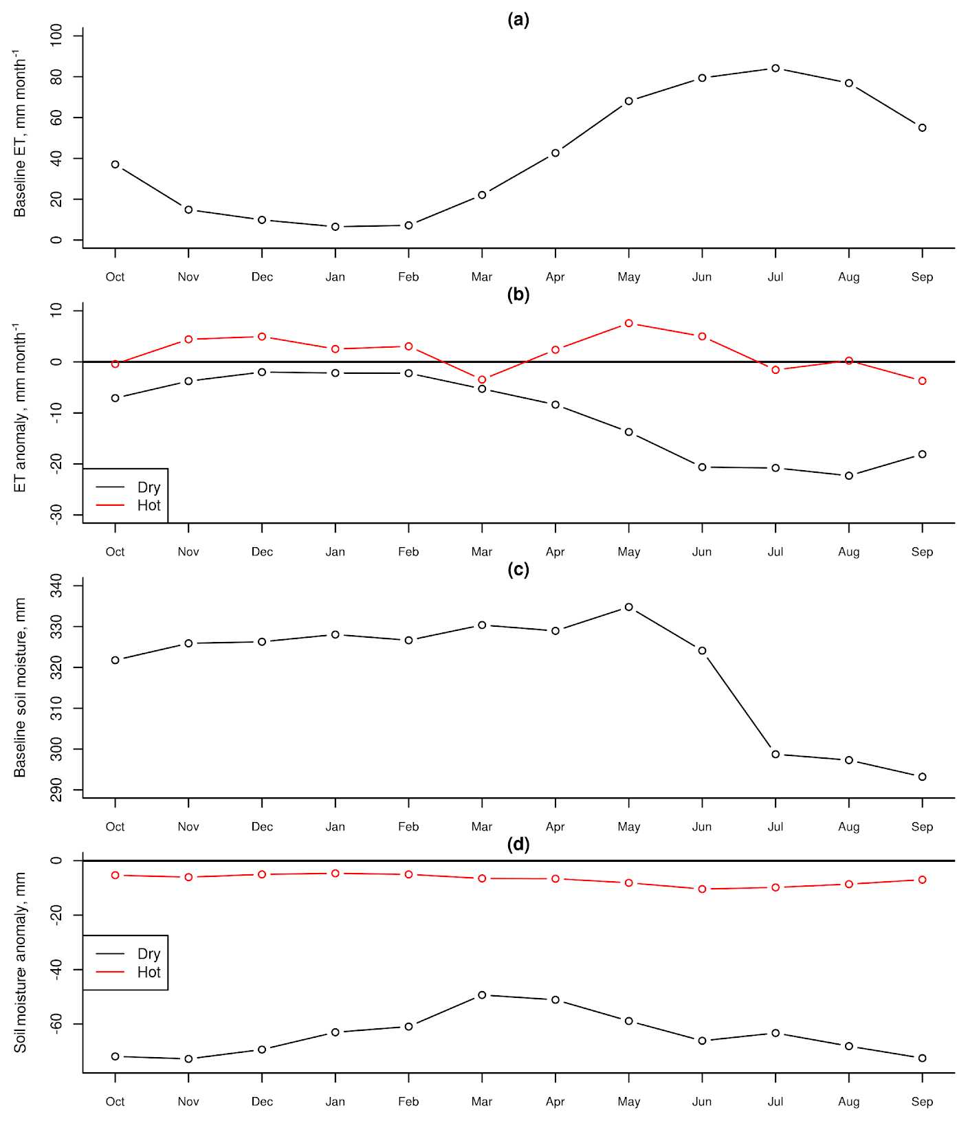
Figure 4Seasonal variability of ET and soil moisture. Panels (a) and (c) show the variables in the baseline runs, while (b) and (d) show hydrologic drought anomalies.

Download

Figure 5 shows a map of ET and soil moisture anomalies in August for the dry run, when the anomalies were highest. The largest ET impacts were localized in the northeast and southeast area, with the west and central parts of the domain being much less affected. The largest soil moisture impacts were localized in the northeast and southwest parts of the domain. There was high variability in ET, with small-scale anomalies up to 10 times the domain average, and in soil moisture, with small-scale anomalies approximately double the domain average. However, while the largest impacts were localized, most of the domain was affected with impacts to ET or soil moisture caused by the meteorological drought forcing.

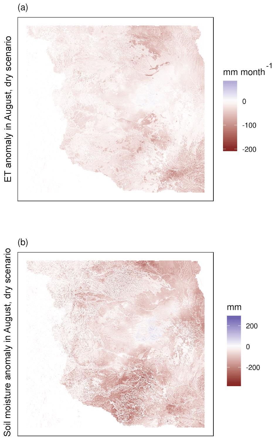
Figure 5Spatial snapshot of drought impacts in August. Panel (a) shows ET anomalies and (b) shows soil moisture anomalies.

Download

This variability illustrates that the average annual temperature or precipitation anomaly is not representative of every snapshot in time, or each individual grid cell. The value of an annual average impact is to capture high-level information about the entire year and the whole domain in a single number which can be used to compare impacts between runs or variables.

3.2 Attribution of drought impacts

The simulated meteorological drought conditions applied in the hot and dry simulations as well as the prescribed land cover changes produced large hydrologic impacts to runoff, ET, soil water content and water table depth. Here we compare the hydrologic impacts of different perturbation combinations to evaluate the relative importance of temperature, land cover and precipitation changes in hydrologic drought impacts. Figure 6 shows domain-averaged annual values of runoff, ET, soil water content and water table depth. Relative to the baseline scenario, most of the drought scenarios have decreased runoff and ET, depleted soil water content, and lowered water tables (i.e., water tables that are further below the land surface), as would be expected in a drought. The exception is the hot and the crops runs, which have slightly higher ET, as discussed later. Figure 7 maps these anomalies across the domain and shows that impacts were typically most severe in the southern and eastern regions. In the central region where rainfall increased slightly (Fig. 3c), this extra water partly avoided the most severe impacts. For example, in the dry and hot–dry runs, soil moisture and runoff anomalies were smaller in this central region.

Figure 6Averages of runoff, ET, soil water content and water table depth, calculated on an annual basis across all cells in the model. Each color represents a different variable and each cluster is a different model run. The baseline, crops and hot runs are generally wetter than the others.

Download

Comparison of single-perturbation runs and multiperturbation runs as shown in Fig. 7 allows the impacts of the drought run to be attributed to individual effects and associated mechanisms. For example, disturbances to land cover produced strong but localized effects. Changing cropland to bare soil stopped transpiration in the affected areas, but increased total ET. Setting plant-covered areas to bare soil stops all transpiration in those cells, but the missing transpiration was more than compensated for by higher ground evaporation in the same seasons. No extra water was available to the system, so (as Fig. 6 shows) the increase in ET was balanced by a small decline in runoff and a small drop in soil moisture and water table levels over the 2 years. Spatially, Fig. 7 shows that most effects were confined to the areas of vegetation change, with the exception of runoff, which decreased in downstream basins.

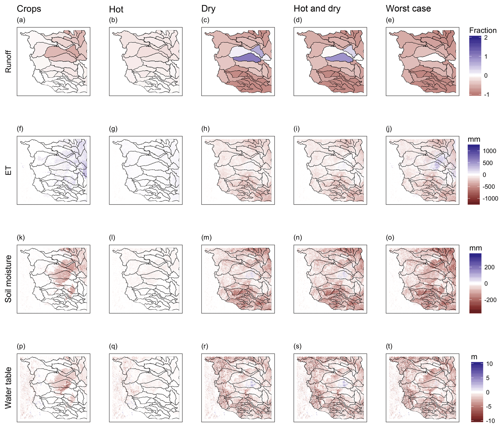
Figure 7Spatial maps of impacts to hydrologic variables, calculated by subtracting the baseline from each run. Each row represents one variable and each column is a different run. Panels (a–e) show runoff, (f–j) show ET, (k–o) show soil moisture and (p–t) show the water table.

Download

(Basins in Fig. 7 are HUC-6 basins such as the North Platte, South Platte, Upper Cimarron, Republican, etc. The HUC or Hydrologic Unit Code system is used to classify drainages in the US.)

Increasing temperature produced small changes in several outputs across the domain. Hotter temperatures increased ET. The increase was limited by available water as many cells remained close to their baseline ET regardless of the temperature increase. Figure 7 showed that runoff decreased by about 10 % while soil moisture and water table levels remained almost the same as the baseline run.

Lowering precipitation drastically reduced all components of the water budget. Spatially, ET and soil moisture anomalies were largest where precipitation deficits were also largest. The exception was along riparian corridors where streamflow and lateral convergence of groundwater maintained local soil moisture and supported ET (Fig. 7). The larger impacts of precipitation relative to temperature are indicative of a water-limited system as would be expected for the High Plains.

It is important to note that the anomalies in the single-perturbation runs shown in Fig. 7 have high spatial variance. Variability in the sensitivity to the applied drought anomalies are illustrated in Fig. 8, which plots the response of individual grid cells to a given forcing change in temperature or precipitation. Variability in Fig. 8 shows that the same perturbation can result in a wide range of responses. Figure 8 also shows these anomalies do not follow a simple functional relationship, which suggests that the ET anomaly for any particular cell is influenced by many other variables. Since ET is controlled by soil and vegetative resistance, soil type and land cover would be possible controls. However, Fig. 8a and b show the anomaly colored by soil type, demonstrating that the wide range is not strongly correlated with soil type. Fig. 8c and d show the same for vegetative cover.

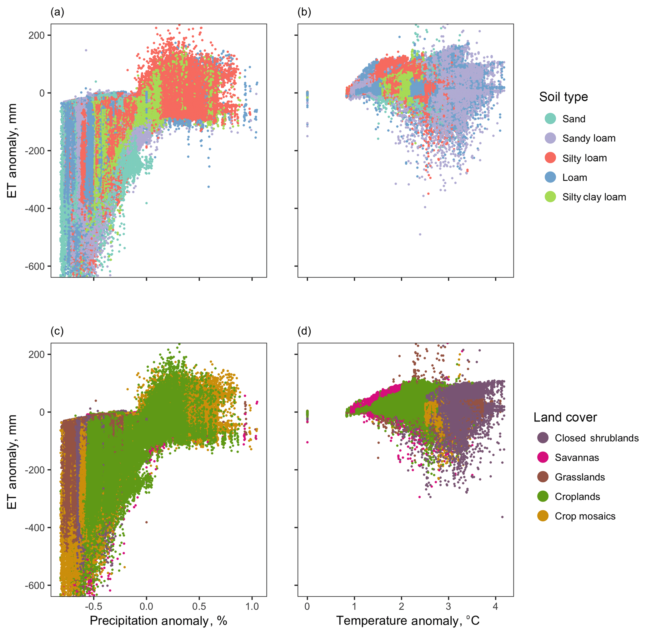
Figure 8Impacts for a given forcing span a wide range, independently of land cover, as shown in (a) and (b), or soil type, as shown in (c) and (d). In (a) and (c), annual anomalies from the dry run are plotted versus precipitation anomaly. In (b) and (d), annual anomalies from the hot run are plotted versus temperature anomaly.

Download

Overall, this demonstrates that decreasing precipitation caused the largest anomalies of any of the single factors. Relative to precipitation, temperature produced minor changes, especially in runoff. Vegetation change from crops to bare soil had large impacts on the local areas, but an intermediate effect when averaged over the domain as a whole. This applies to the relative size of the changes studied; a 2 ^∘C increase in temperature versus a 40 % drop in precipitation (when summed over the domain) and disturbance to land cover over about 30 % of the model area. For individual grid cells, anomalies followed the expected pattern, with heat causing ET to increase and dryness causing it to decrease. The size of the anomalies, however, were relatively unpredictable even when controlling for the forcing change, soil type and land cover.

3.3 Factor combinations

Section 3.1 presented the overall hydrologic impacts of individual and multiperturbation runs. This section quantifies how these factors combine and interact. In a completely linear system, the single-perturbation impacts would combine additively to equal the multiperturbation impacts; however, because hydrologic systems are non-linear and there are many system components interacting simultaneously, some part of that total may also be due to interactions between the factors. Consideration of important mechanisms includes land cover change and water-limited behavior. In general, individual factors can combine in a nonlinear way. For example, hotter temperatures occurring alone should increase ET, and drier weather alone should decrease ET, as detailed in the introduction. If hot and dry weather occurs, the total impact to ET could be a combination of the individual impacts. There could also be an interaction between the factors in which the change due to one perturbation depends on the level of the other factor. For example, the increase in ET due to temperature could depend on the amount of precipitation (which is a major control on available soil water) (e.g., Livneh and Hoerling, 2016).

Figures 9 and 10 compare the impacts of the single-perturbation runs with those in the multiperturbation runs. Each figure compares the result of a multiperturbation run with the combination of single-perturbation runs. In a perfectly linear system, the two results would be the same. Instead, the figures show that impacts of each multiperturbation run can be attributed to individual components, but not completely. For example, Fig. 9 shows that ET impacts predicted by adding the impact in the hot run (a 21 mm yr⁻¹ increase) to the impact in the dry run (a 126 mm yr⁻¹ decrease) predict a combined effect in the hot–dry run of 105 mm yr⁻¹ decrease. This amounts to 93 % of the 114 mm yr⁻¹ decrease that was actually modeled in the hot–dry simulation. Similar patterns hold for the other variables, with the dry run contributing more than the hot run to every anomaly, as observed qualitatively in the previous section. In Fig. 10, a similar analysis shows that the hot–dry run contributes almost three times as much as the crops run to each anomaly. The figures also show that the individual components do not account for the entire effect. For example, in Fig. 9 the hot–dry run is lacking 9 mm yr⁻¹ of ET and keeps an extra 9 mm yr⁻¹ of runoff compared to what would be expected by combining individual impacts calculated in the hot run and the dry run.

Figure 9Modeled anomalies between experimental runs and the baseline are shown for the hot–dry run, the hot run and the dry run. The anomalies in the hot–dry run are close to the sum of those in the hot run and the dry run. This linear behavior is most true for soil water content, less so for ET and runoff.

Download

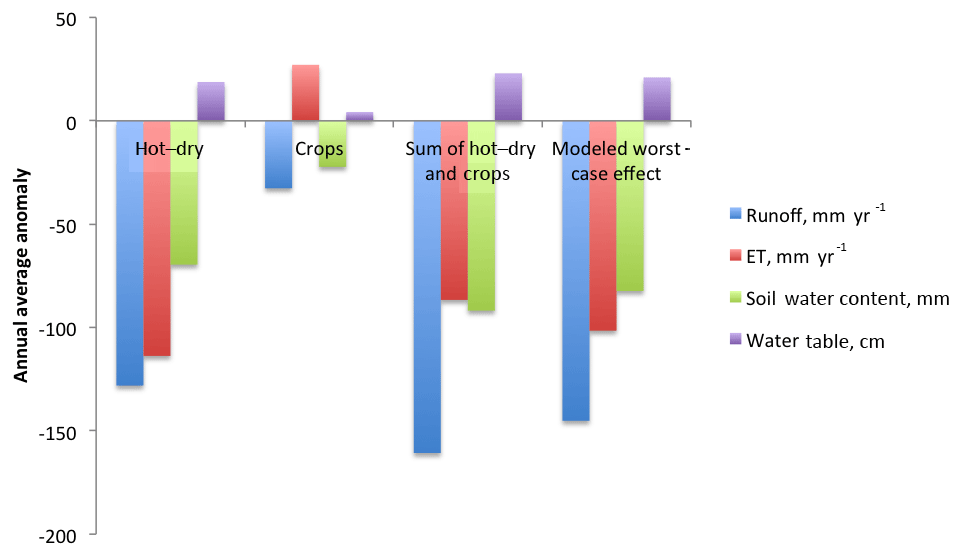
Figure 10Modeled anomalies between experimental runs and the baseline are shown for the worst-case run, the hot–dry run and the crops run. The anomalies in the worst-case run are close to the sum of those in the hot–dry run and the crops run; the largest difference is seen in runoff.

Download

These runs show the impact of land use on hydrologic drought as it develops in response to meteorological drought. Figure 10 shows that the hot–dry run lowered ET by 114 mm yr⁻¹ and dried soils by 70 mm on average, when drought occurred with no land use changes. However, in the worst-case run where meteorological drought was combined with removal of crops, ET was lowered less (102 mm yr⁻¹) and soils were dried more (82 mm). The directions of these changes are consistent with the impact of land use alone: removing crops without drought increased ET by 27 mm yr⁻¹ and dried soils by 22 mm. Vegetation removal exacerbates the drying effects of drought on soil because the presence of vegetation shields soil from evaporation, but since there is limited total moisture, the two effects do not add linearly and the soil moisture decrease is capped at 82 mm instead of 70 mm + 22 mm = 92 mm in the worst-case run. Similarly, vegetation removal tends to increase ET because more is evaporating from the soil, but drought decreases ET because less water is available in general. These water limitations may relate to nonlinear behavior as discussed later in the paper. The worst-case run has less impact on ET at the expense of drier soils when compared to the hot–dry run.

It is instructive to examine the mismatch between modeled anomalies and those predicted by linearity using spatial plots. Figure 11 maps this nonlinearity across the domain for runoff, ET, soil moisture and the water table. The left-hand column compares the hot–dry run to the individual hot and dry runs, and the right-hand column compares the worst-case run to the hot–dry and crops runs. The nonlinearity is calculated as a percent difference, as described in the Methods. Red colors mean that the multifactor impact was smaller than expected, while blue colors mean that it was larger. Gray denotes a small number of outlier grid cells. On average in the hot–dry run, ET generally decreased more than predicted by linearity, and runoff decreased less, while the water table and soil moisture decreased less in the center, and more in the north and south. Nonlinearity between the worst-case run compared to the hot–dry run was naturally localized to the areas of land cover disturbance (i.e., where there were differences between the two). Runoff changed in either direction, ET generally decreased more than predicted by single-factor runs, and soil moisture and water table levels decreased less than the combination of their single-factor run impacts. Importantly, the nonlinearity spans a wide range of variation, with simulated multiperturbation impacts being up to ±40 % from the expected values in a linear system.

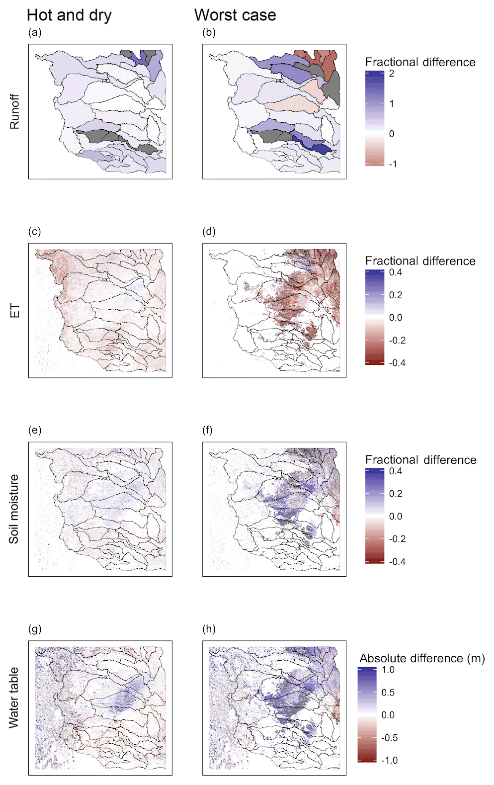
Figure 11Nonlinear behavior in both multiperturbation runs shows spatial patterns. Panels (a) and (b) show runoff, (c) and (d) show ET, (e) and (f) show soil moisture, and (g) and (h) show water table levels. Panels (a, c, e, g) compare the hot–dry run to the single-perturbation hot and dry runs. Panels (b, d, f, h) compare the worst-case run to the crops run and the hot–dry run.

Download

Antecedent soil moisture and water-limited behavior may explain some of the nonlinearity shown in Fig. 11. Figure 12 shows the modeled ET anomalies versus antecedent soil moisture for a given forcing change (color scale), providing a general illustration of these mechanisms within the model. Figure 12a shows the dry run and Fig. 12b shows the hot run. In this figure, all cells are plotted regardless of soil texture. This is a slight simplification as soil texture changes water retention, so two soils with the same water content but different textures might have different amounts of water available for evaporation. Thus, in a few cases, the same water content might lead one cell to be energy limited but another to be water limited, as the demand for evaporation exceeds the available water. This does not change the overall finding that pre-existing soil moisture partially controls the response of model cells to forcing changes. The transition in both panels at about 350 mm of soil water content indicates the importance of antecedent soil moisture. Above this transition point, increasing temperature produces the largest increases in ET. Decreasing precipitation produces only small anomalies, because enough water is available in the wettest cells to supply the continued ET demand. Below this point, however, the system is water limited. In the presence of a temperature increase, soil water content limits the possible ET increase. These observations from the single-perturbation runs support a mechanism for the nonlinearities that has been suggested in previous research (e.g., McEvoy et al., 2016; Seniviratne et al., 2010): when precipitation decreases, there is less available water to supply ET demand even when a rising temperature increases potential ET. Thus the simulated multiperturbation ET is smaller (in other words, the deficit in ET is larger) than would be expected by simply combining factors.

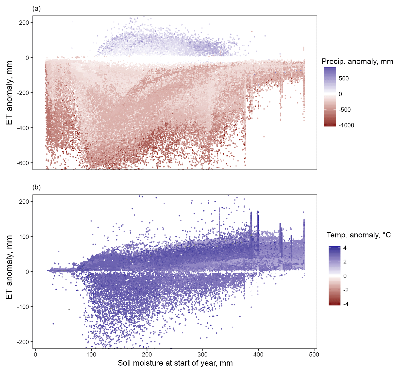
Figure 12Antecedent soil moisture is an important control on model ET response. The ET anomaly is plotted versus antecedent soil moisture and colored by model forcing. (a) shows data from the dry run (color scale is precipitation change) and (b) shows data from the hot run (color scale is temperature change). Each point is one model cell. Below about 350 mm of soil water content, the cells show water-limited behavior in which drought causes decreased ET depending on severity.

Download

A final possible explanation is that the nonlinearity is an artifact of the modeling. This model captures important processes of the hydrologic cycle using physically based equations, as discussed in the Methods. Additionally, all runs were conducted with the same modeling environment and compared to a baseline from that model. However, we acknowledge there could be additional nonlinearities and feedbacks in the system that are not captured in our model.

3.4 Importance of spatial scale

This section examines the importance of scale in assessing these processes. Impacts of individual factors show less variability and more dependence on model forcing at larger scales. As was discussed in Sect. 3.1, impacts of individual factors can be more variable at small scales (Fig. 8); in other words, a given forcing change can produce a wide range of impacts to ET. Figure 13 shows that this variability is greatly reduced as soon as ET anomalies are aggregated to small (HUC-8) drainage basins. By the time the ET response is aggregated to subcontinental watersheds on the scale of the Arkansas or Red rivers, these spatial differences cancel out and variability is greatly reduced.

Figure 13Impacts of individual factors become less random at larger scales. (a) shows ET anomalies of the dry run and (b) shows ET anomalies of the hot run, plotted against their respective forcing anomalies. Impacts begin at the individual cell level and are aggregated to a series of larger scales.

Download

Section 3.2 showed that nonlinearity (i.e., the portion of the response not accounted for by the linear combination of the individual perturbations) can span ±40 % for a given grid cell (Fig. 11) while being much less at the entire domain scale (Figs. 9 and 10).

Figure 14 examines this nonlinearity across a variety of spatial scales, comparing the multifactor hot–dry run to the single-factor hot and dry runs. The box plots show the spread of the data plotted in the left-hand column of Fig. 11, averaged at several different scales. Overall, Fig. 14 shows that the nonlinearity is much decreased in moderately sized (HUC-6) river basins, and small in subcontinental river basins. (HUC-8 basins are smaller basins that nest within HUC-6 drainages. The term major basins is used here to mean the Arkansas, Red and Missouri subcontinental basins.) This is especially important because it shows that treating the system as linear would fail to capture the most severe impacts occurring in individual grid cells. Closer inspection of Fig. 14 shows that the median nonlinearity becomes more positive for runoff and more negative for ET as scale increases. In a subcontinental basin as a whole, there is a small positive nonlinearity in runoff, meaning that the change in runoff under both temperature and precipitation increases is slightly larger than that due to the separate effects of temperature and precipitation. The interpretation that responses are more linear at larger scales focuses not on the median magnitude, but rather on the decreasing interquartile range of the box plots at larger scales.

Figure 14Factors combine in a more linear way at larger scales. The multifactor hot–dry run is compared to the single-factor hot and dry runs. Each panel shows box plots that characterize deviations from linearity in the hot–dry run from model cell to subcontinental scales. Panel (a) shows runoff, (b) shows ET, (c) shows soil water content and (d) shows the water table.

Download

The previous two figures may seem to contradict the message of earlier sections. They suggest that model responses at large scales are basically linear and predictable from the single-factor runs. If the impacts of individual factors are actually straightforward and combine in a basically linear way at subcontinental scales, perhaps simplified models would be adequate to answer big-picture questions at large scales without involving the full complexity of an integrated hydrologic model. The free-draining run provides insight to address this question by removing interactions between cells. Without lateral flow, a free-draining run can be considered as a package of single-column models, run across a spectrum of soil types, slopes and land cover.

The free-draining run allows us to directly test the impact of lateral flow on the simulated drought response across spatial scales. We find that the simulated changes from the land cover change simulation vary significantly between the standard and free-draining runs. As previously noted, ET tends to increase when croplands change to bare soil. Figure 15 compares ET in the worst-case simulation to a baseline in both the free-draining and typical configurations. Inspecting the area of crop disturbance in Fig. 15b confirms that in the normal model configuration, ET increases in the locations where crops change to bare soil. However, in the same area of the upper panel, exactly the same forcing changes cause ET to decrease for the free-draining run. This is largely explained by the nature of the free-draining run. In the normal configuration, lateral flow of groundwater can sustain ET and soil moisture, similar to the results found by Maxwell and Condon (2016). However, when no lateral flow is allowed, every grid cell is restricted to the soil moisture within it.

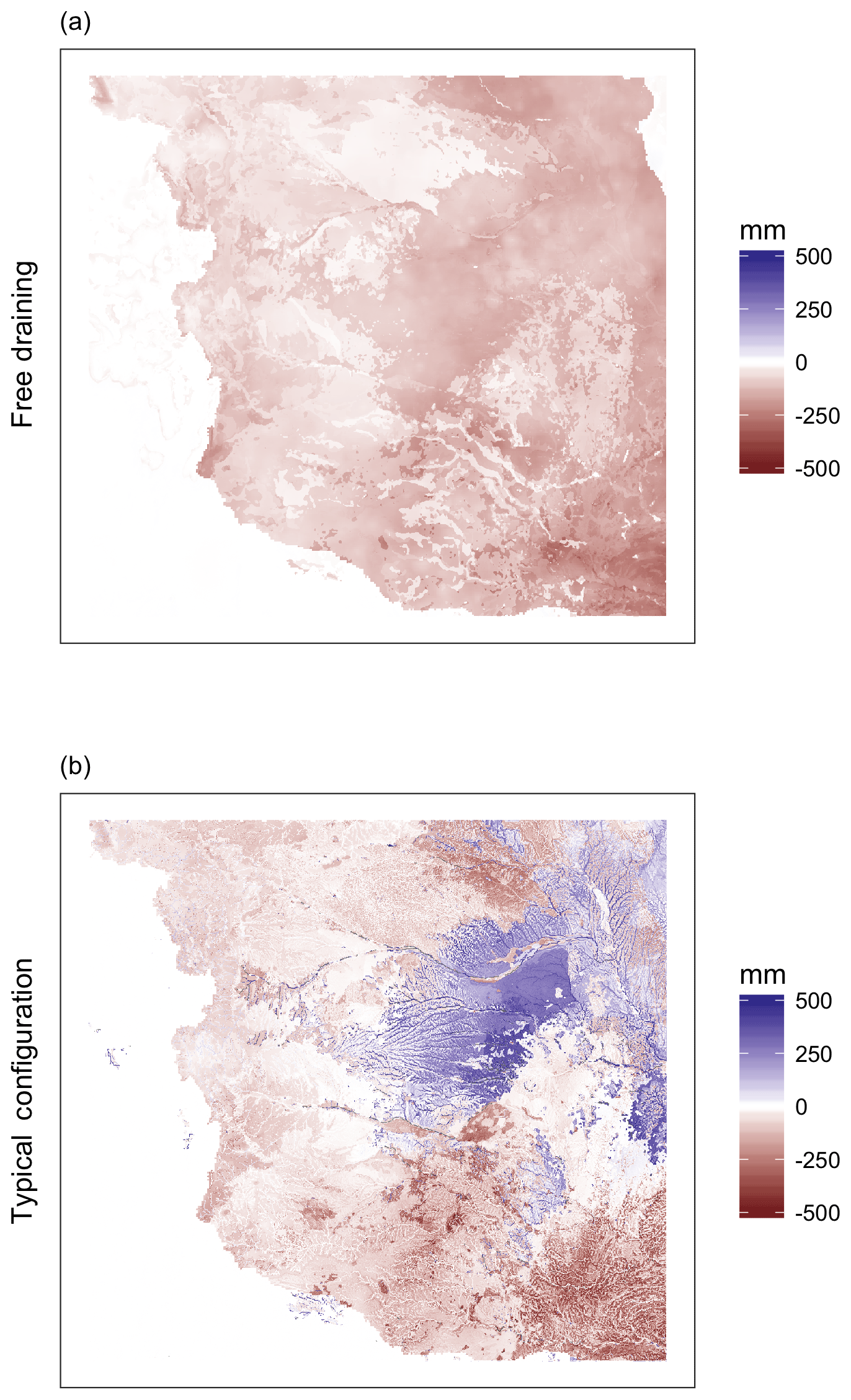
Figure 15Large-scale impacts of crop changes depend on representation of small-scale processes. Spatial maps are calculated by subtracting (a) the free-draining baseline (run 2) from the free-draining worst-case run (run 8) and (b) subtracting the baseline with lateral flow (run 1) from the worst-case run (run 7). Panel (a) shows the free-draining run where ET decreases in areas of land cover disturbance. Panel (b) shows the typical configuration for comparison, where ET increases in areas of land cover disturbance.

Download

The difference may also be due to the differences in water table between the simulations, as the free-draining run did not use a constant water table or a separate spinup for the free-draining run, and therefore it has a lower water table than the other runs. (Impacts were calculated by comparison to the free-draining baseline run, which will partially adjust for this. However, it is still possible that a generally lower water table resulted in a water-limited system and decreased ET once plant transpiration stopped.) The results of the free-draining run relate to the third research question on spatial scaling and complexity by showing that even linear-seeming, large-scale predictions depend on representation of lateral flows and interactions within the model.

Overall, this section shows that nonlinear kilometer-scale impacts aggregate to large-scale changes which can be well predicted by linear combinations of single-factor simulations. The complexity of model response depends on the scale of the area of interest, with individual kilometer-scale grid cells being complex and aggregated subcontinental river basins response being much more simple. Responses at any scale nonetheless depend on representation of the processes and feedbacks at smaller scales. At coarse resolution, single-factor simulations may provide usable results; but as the resolution increases, accounting for the nonlinearities arising from multiple factors becomes more important. This means that coarser-scale simulations such as those often run on VIC may capture big-picture drought-related impacts, but may miss the finer-scale local variation.