3.1 General workflow

The aim of this study is to elucidate the application potential of a process-based hydrological model for water resources and drought prediction. Consequently, hindcasts of reservoir volumes and hydrological drought indices shall be produced, driving the model by meteorological hindcasts. The general workflow is illustrated in Fig. 2.

Figure 2Workflow for the generation and evaluation of hindcasts of hydrological drought indices.

Download

A process-based hydrological model was first calibrated to observations and an initial model run conducted for the period of 1980 until 30 June 2014. This initialisation run was driven by observed meteorology and at each 1 January the storage volume of each strategic reservoir was replaced by the observed value. Furthermore, if available, measured reservoir releases through a dam's intake devices were fed into the model in order to make use of as much information as available to produce simulations as realistic as possible. The first year of the run was used as a warm-up to bring the model states into equilibrium. At each end of year, the model's state variables, including soil moisture, groundwater, river, and small (i.e. non-strategic) reservoir storages, were stored. This entire procedure is intended to mimic the conditions in a real forecast situation.

In a specific hindcast run, the model was then re-initialised with the saved model states and driven by hindcast meteorology. These runs were conducted successively for the wet seasons (1 January to 30 June) of 1981 to 2014. The resulting strategic reservoir volumes were used to infer drought indices which were evaluated employing verification metrics. To distinguish uncertainties from the meteorological hindcasts and in order to investigate mere model performance, the model runs were performed in two ways: driven by observations (simulation mode) and meteorological hindcasts (hindcast mode).

The runs were conducted for both the process-based model initialised and calibrated within this study and a statistical model, which is a regression approach derived by Delgado et al. (2018b) for the same study area. Consequently, verification metrics were calculated and analysed for both model approaches and both forcing modes.

In order to identify the strengths and weaknesses of the process-based model, the results of the simulation runs were further analysed. In this context, the model output (reservoir storage) was stratified. The details of the individual processing steps are described in the following.

3.2 Data

To parametrise the hydrological model, various spatial data were obtained including a 90 m × 90 m SRTM digital elevation model (DEM), a soil map provided by the Research Institute for Meteorology and Water Resources of the state of Ceará (FUNCEME) along with soil parameters from a local database (Jacomine et al., 1973) from which the necessary model parameters were calculated employing pedotransfer functions, a land cover map from the Brazilian Ministry of the Environment with parametrisations assembled by Güntner (2002), and a map of small and strategic reservoirs provided by FUNCEME. Reservoir parameters were made available by the Company for Water Resources Management of Ceará (COGERH) and FUNCEME and include the year of dam construction, storage capacity, and water-level–lake-area–storage-volume relationships along with daily resolution time series of water levels and artificial water release. A time series of daily precipitation for 380 stations within and in close vicinity around the study area were provided by FUNCEME. Other daily meteorological time series needed by the model (relative humidity, air temperature, and incoming shortwave radiation) were derived from the gridded dataset (0.25^∘ × 0.25^∘ resolution) of Xavier et al. (2016).

3.3 Meteorological hindcasts

Daily meteorological hindcast data for the period 1981 to 2014 used as input into the hydrological model stem from an ensemble (20 members) of ECHAM4.6 GCM runs (Roeckner et al., 1996) which were bias corrected by empirical quantile mapping (EQM) (Boé et al., 2007; Gudmundsson et al., 2012). Although Delgado et al. (2018b) identified some deficiencies regarding this product, there was no clear better-performing alternative. In addition, ECHAM4.6 is already employed operationally by the local water authority FUNCEME (Sun et al., 2006), and, in contrast to other seasonal forecast systems like those by ECMWF, it comes without further costs for operational use, making it the candidate for future operational application. The 20-member ensemble runs of ECHAM4.6 were conducted and results provided by FUNCEME. More information is given in Delgado et al. (2018b).

3.4 The process-based model

3.4.3 Analysis of simulation performance and influencing factors

An objective of this study is to analyse the simulation performance of the process-based model in more detail and to identify possible influencing factors. Instead of using a single goodness of fit measure, as for automated calibration, different aspects of model performance should be investigated. Therefore, the Kling–Gupta efficiency (KGE) was chosen as a performance measure along with its three components correlation, bias, and deviation of standard deviations of simulations and observations (see upper part of Table 1). Like NSE and BE, KGE scales from minus infinity to one where one is the optimum value achieved for maximum correlation (i.e. COR=1) and no deviation of means and standard deviations. To assess which factors influence the model performance, several candidate descriptors where selected, which are presented in the lower section of Table 1. These descriptors were tested for their capability to explain model performance in time and space in a regression approach by using these descriptors as predictors and the performance metrics as the response variable.

(Gupta et al., 2009)

Table 1Response and predictor variables used for the analyses of the process-based model performance.

Download Print Version | Download XLSX

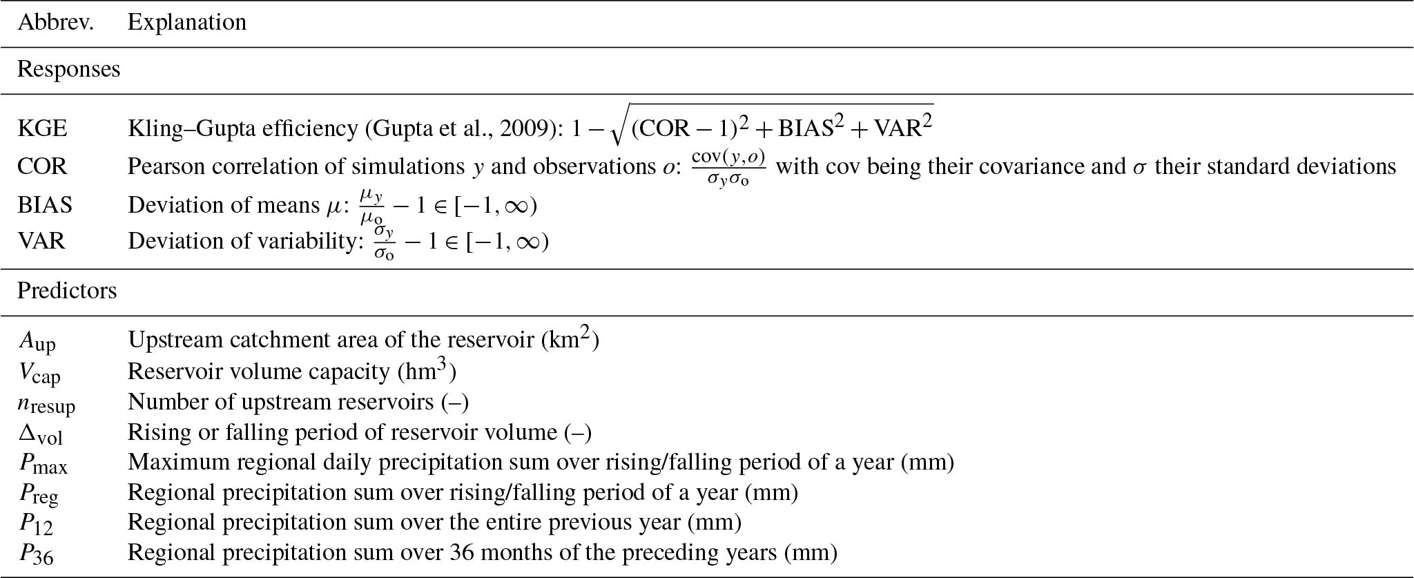
For the analysis, the calibration period 2003 to 2010 was used. Each response variable (i.e. performance metric) was calculated for each of the 36 strategic reservoirs located in the study area. Furthermore, each year was divided into a falling period, where the difference of reservoir levels for two consecutive days was negative, and a rising period, where the difference was greater than or equal to zero. For each reservoir, year, and period, the respective performance was computed and analysed separately. This resulted in a total of 32 reservoirs times 8 years times two periods minus some missing observations, i.e. 484 values to be aggregated for each response variable. The predictors were either static and unique for each reservoir (upstream catchment area A_up, reservoir capacity V_cap, number of upstream reservoirs n_resup), region-specific and dynamic as aggregation over a certain amount of time (maximum daily precipitation P_max, regional precipitation sum P_reg, regional precipitation over the last 12 months P₁₂, and over the last 36 months P₃₆), or a grouping variable by itself (reservoir level is currently rising or falling Δ_vol) (see also Table 1 for more information).

To identify predictor importances and their specific influence on the performance measures, a random forest analysis was conducted using the R package party (version 1.3-1). In general, random forests consist of an ensemble of regression trees, where each tree is fitted using a bootstrap sample of the training dataset and only a subsample of all available predictors. This eliminates typical problems of traditional regression tree approaches, such as a high sensitivity to small changes in the data and the likelihood of overfitting (Breiman, 2001). For this study, a refined random forest algorithm was employed, which is better suited for predictors of different types (e.g. mixed categorical and continuous) and produces more robust measures of predictor importance in the case of correlated predictor variables (Hothorn et al., 2006; Strobl et al., 2007, 2008).

For each response variable, an individual random forest was built. Except for Δ_vol (categorical), each predictor and response variable was treated as numerical. To generate robust estimates of predictor importance, 1000 regression trees were built per forest (otherwise standard parameter values of the algorithm were used). The most influential predictors for a certain response were then distinguished by an importance measure, which in this study was derived by permuting the values of each predictor and measuring the difference in prediction accuracy of the random forest before and after permutation (also termed permutation importance in contrast to the often used Gini importance or mean decrease in impurity). In addition, the permutation of predictor values was done by accounting for potential correlation among predictor variables (hence termed conditional permutation importance) as suggested by Strobl et al. (2008).

In order to get an impression of the concrete effect of each predictor instead of the mere variable importance, the two leaf nodes with the highest and lowest median response values for each tree were identified. For these two nodes, the ranges of each numerical predictor (except Δ_vol) were classified into four groups ranging from small to large to facilitate visual investigation.

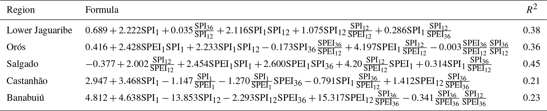
Table 2Regional equations used for the calculation of monthly volume changes with the statistical approach. Table extracted and extended from Delgado et al. (2018b) (Table A1). For details and abbreviations see text.

Download Print Version | Download XLSX

3.5 The statistical model: a regression approach

A goal of this study is to answer the question of whether the application of a complex process-based simulation model is worthwhile in comparison to a much more convenient statistical approach to generate seasonal forecasts of reservoir storage and drought indices. To achieve this, the regression model of Delgado et al. (2018b), which was developed for the same study area, was employed. They fit a multivariate linear regression (MLR) model individually for each of the subregions also defined in this study. As a response variable, regional volume changes were used (approach M2 in Delgado et al., 2018b). As possible predictors, meteorological drought indices (standardised precipitation index, SPI; and standardised-precipitation–evapotranspiration index, SPEI) aggregated over time periods of 1, 12, and 36 months, respectively, were considered in their study. To account for correlation among predictors, ratios of predictors exhibiting significant correlation to each other were used. Genetic optimisation with respect to the Akaike information criterion (AIC) was employed to determine the specific predictors for each subregion. To enforce model parsimony, not more than five predictors should be used in the regression equation. For the model fit, all available observations within the analysis period were used (monthly values from 1986 to 2014, less a few missing values). The resulting equations are presented in Table 2.

To generate hindcasts, the predictors of the equations (the SPI and SPEI values over different time horizons) were calculated on a monthly scale to obtain monthly forecasts of regional reservoir volume changes for each rainy season of the hindcast period. Regional storage volume values could then be obtained by successively adding predicted volume changes to the measured value of December of the previous year, which served as a base value for each rainy season. Even though the shown model fits for monthly volume changes were rather poor (low R² values in Table 2), the derived absolute reservoir level values were in good agreement with measurements (Delgado et al., 2018b).

To compare the mere simulation performances, both the process-based and the statistical model were first driven by observed meteorology to exclude the effect of the downscaled GCM runs. In a second step, the two approaches were evaluated for real hindcasts.

3.6 Drought hindcasting

4.1 Comparison of model performance in simulation mode

Figure 3 compares the performances of the process-based and statistical model in simulating relative regional reservoir storage driven by observed meteorology. The regional RMSE varies between 5 % and 18 %, whereas for the whole catchment both modelling approaches achieve a result of about 13 %. Overall, the performance differences between the two models are small for all regions. Only for Salgado the statistical model shows a lower RMSE compared to the process-based model, and the difference among the two approaches is largest (6 %). For all other regions, the process-based model exhibits a slightly higher accuracy, and the interregional ranking is equal for both approaches. Generally speaking, both models show a comparable performance, suggesting they are equally suitable for their application in hindcast mode.

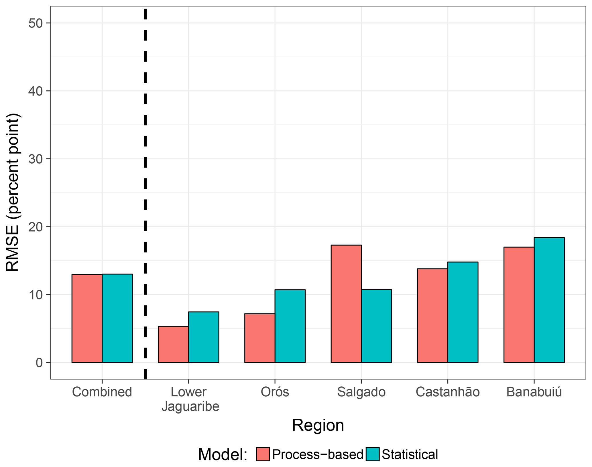
Figure 3Comparison of accuracy in predicting relative reservoir storage for the process-based and statistical model in simulation mode (i.e. run with observed forcing). The underlying analysis period comprises monthly values of the rainy season (January to June) over the hindcast period (observations available since 1986 until 2014 with some data gaps in between, resulting in a maximum of 174 values for each subregion).

Download

4.2 Comparison of model performance in hindcast mode

The uppermost panel of Fig. 4 shows that, in hindcast mode, the accuracy in terms of RMSE considerably decreases when compared to simulation mode for both types of models. However, in contrast to the situation in simulation mode, the statistical approach outperforms the process-based model for all regions. While for the statistical model deterioration in terms of RMSE is generally less than 10 %, the process-based model achieves significantly lower accuracy with increasing RMSE by up to almost 30 %. This degradation of model performance in hindcast mode for the process-based model is especially pronounced for the Banabuiú region.

Figure 4Model performance in hindcast mode for the two model approaches. In the top panel, horizontal dashed lines in the bars mark the results obtained with observed forcing (simulation mode, as in Fig. 3). Note that for RMSE low values indicate a better performance while for ROCSS and BSS higher values are favoured.

Download

The lower two panels of Fig. 4, however, demonstrate that both approaches are able to generate drought hindcasts with skill. The resolution of event hindcasting of the two models (i.e. the ROCSS) is very similar when it is combined over the whole catchment. Regional differences are more pronounced but still negligible. For some regions the process-based model performs better, but for other regions the statistical model performs slightly better. The BSS, while also indicating skill, shows lower performance values which can be attributed to lack of accuracy (as already indicated by RMSE) and reliability.

An attribute plot, as the one presented in Fig. 5, can reveal more details on that issue. Therein, the predicted probability of drought occurrence (obtained from the outcomes of individual ensemble members) is plotted against the relative frequency of observed drought occurrences (solid lines) together with the relative prediction frequency of a certain forecast probability interval (dotted lines). It demonstrates several verification attributes including resolution (the flatter the solid lines, the less resolution), reliability (agreement with the gray diagonal line), sharpness (dotted coloured lines), and skill (values within the gray region contribute positively to BSS; for unclear terms see Appendix Sect. Appendix A or consult textbooks such as Wilks, 2005). Apparently, predictions from both models contain skill except for low forecast probabilities where both models contribute negatively to BSS. Furthermore it can be seen that both approaches exhibit problems in terms of reliability. Specifically, forecast probabilities are too low compared to observed occurrences, which is generally denoted as underforecasting. This observation appears to be a bit more pronounced for the process-based model than for the statistical model. That also holds true for sharpness, as the statistical approach shows slightly more confidence for higher forecast probabilities; i.e. the relative frequency of maximum forecast probability is higher.

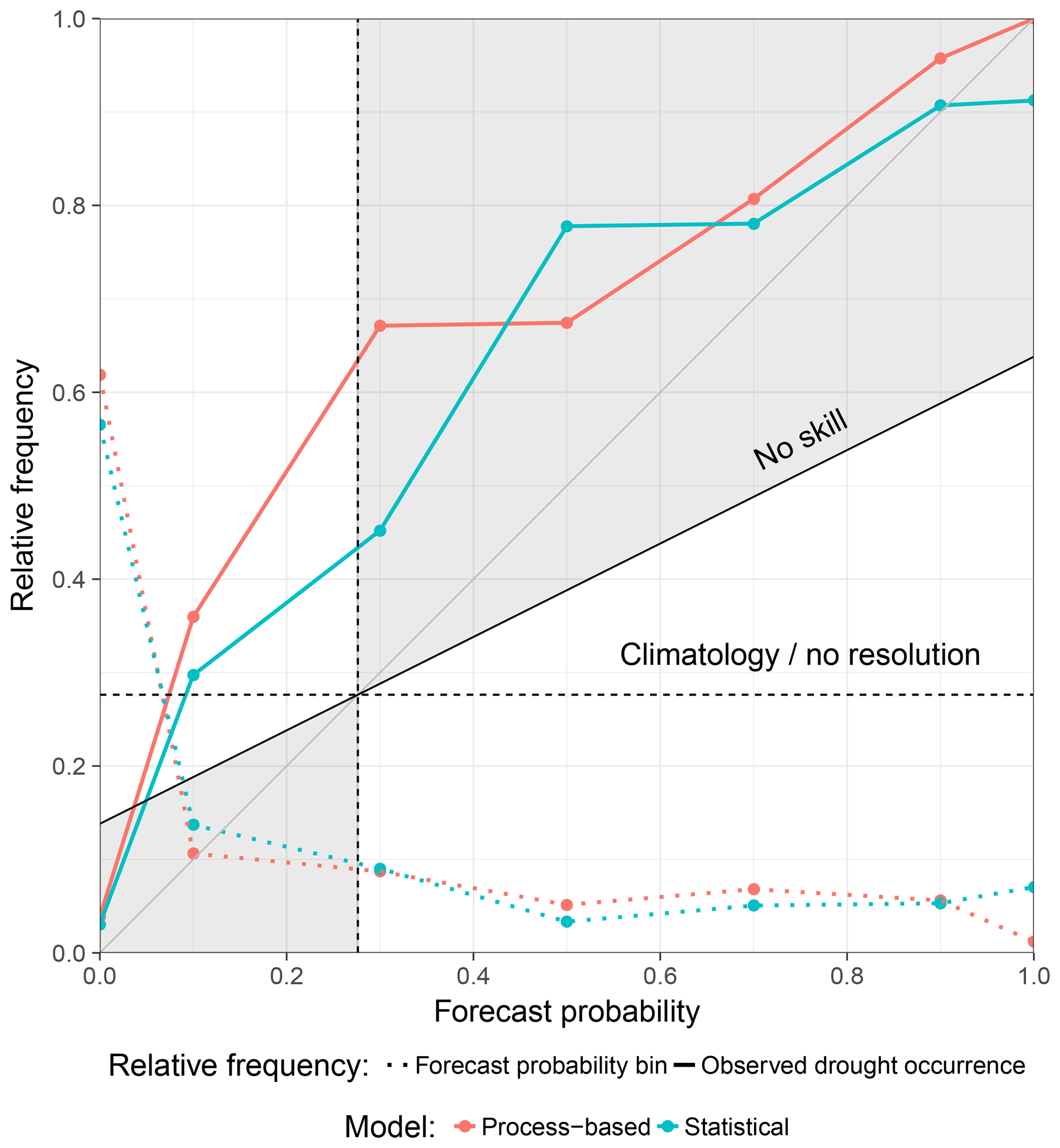
Figure 5Attribute plot of drought hindcasts aggregated over the whole study area. Values within the gray region contribute positively to the Brier skill score (BSS). For details on the interpretation of the plot see text.

Download

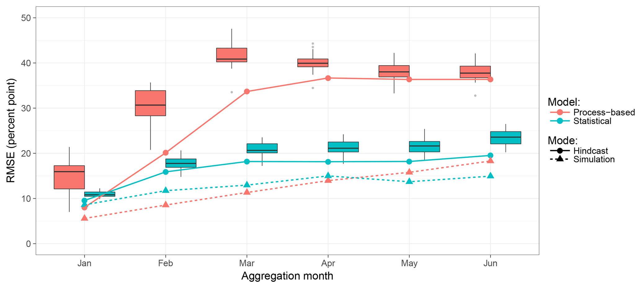
Figure 6RMSE of regional reservoir storage hindcasts with increasing forecast horizon and lead time. Monthly values are obtained by aggregation over the full analysis period (1986 to 2014) for a specific month. Each box reflects the distribution of the 20 ensemble members. Coloured solid lines refer to the ensemble median taken as the deterministic forecast and analysed individually.

Download

4.3 Model performance attribution

4.3.1 Hindcasts

The monthly aggregated accuracy of the hindcasts, i.e. performance with increasing lead time, is shown in Fig. 6. Overall, the hindcast error (i.e. RMSE) increases with lead time (i.e. progression of the wet season), even when using observed forcing. The statistical approach generally produces better hindcasts. Its RMSEs differ only little from runs with observed forcing. Also the increase in RMSE with lead time is very similar. For the process-based model, hindcasts deviate clearly from observation-based results (as was already shown in Fig. 4). The error increases much more strongly over the hindcast horizon. However, its RMSE values reach a plateau at about 40 % in March. Generally, it can be seen that aggregating the ensemble members by using the median of reservoir storage hindcasts (solid lines) is usually a better choice than most of the single ensemble members (distributions shown as box plots). The spread of ensemble member results differs for the two approaches. These ranges are clearly larger for the process-based model in January and February but comparable for the other months.

In Fig. 7 prediction accuracy is assessed for different wetness conditions (i.e. dry, normal, wet) over different accumulation time periods for rainfall. Again, when driven by meteorological hindcasts, the statistical approach performs best with relatively small differences compared to results obtained using observed forcing. Under wet conditions, irrespective of the rainfall accumulation period, the error is highest for most settings. The only exception from this pattern shows the process-based model driven by hindcasts. Here, the error under dry preconditions increases with increasing rainfall accumulation length while the performance under wet preconditions improves with longer accumulation length.

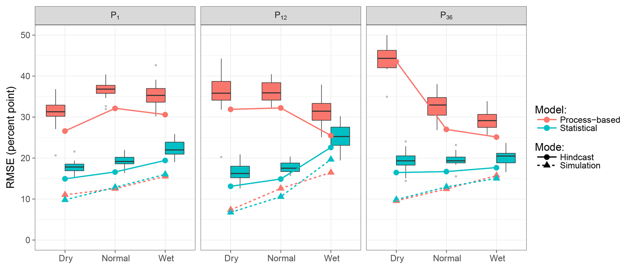
Figure 7RMSE of regional reservoir level hindcasts for different antecedent wetness conditions. Wetness is expressed by three different accumulation horizons of rainfall (1, 12, and 36 months; left, centre, right). Each box reflects the distribution of the 20 ensemble members. Coloured solid lines refer to the ensemble median taken as the deterministic forecast and analysed individually.

Download

4.3.2 Process-based simulation performance

In the preceding subsections it was shown that the process-based model does not outperform the statistical approach. Moreover, in hindcast mode, the process-based model often achieved worse performance measures, especially in terms of accuracy. This subsection therefore aims at the identification of deficit causes by analysing the results of process-based model calibration and potential influencing factors of simulation performance in more detail.

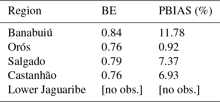
Regional calibration performance of the process-based model is summarised in Table 3. A good overall agreement of simulated and observed reservoir dynamics in terms of BE values could be achieved during calibration. However, percent bias (PBIAS) as a performance metric not used in the calibration shows, on the one hand, acceptable values of no more than 12 % but, on the other hand, a consistent slight overestimation of reservoir level dynamics. It can be further observed that a good BE value does not correlate with a low PBIAS.

Table 3Results of regional calibration of the process-based model. BE refers to benchmark efficiency (Eq. 1) and was used for calibration; PBIAS is percent bias, i.e. the average tendency for over- or underestimation of simulations in comparison to observations. For Lower Jaguaribe, no observations at the catchment outlet were available.

Download Print Version | Download XLSX

The random forest analysis brought more insight into process-based model performance and its influencing factors. Figure 8 illustrates the importance of each potential predictor for different performance metrics. Apparently, overall model performance (here measured via KGE) primarily depends on the wetness preconditions (P₃₆). While reservoir size (V_cap) plays only a minor role for the overall performance metric KGE, it clearly affects correlation and bias. (Mis)match of standard deviation (VAR), however, is mainly determined by both wetness conditions and reservoir size. Overall, long-reaching antecedent wetness condition (P₃₆) is more important than the conditions of the preceding 12 months (P₁₂), and reservoir capacity (V_cap) is dominant over upstream catchment area (A_up), although the latter is not negligible. The current rainfall conditions, in terms of intensity (P_max) and sum over a rising/falling period (P_reg), whether it is a reservoir level increase or decrease period (Δ_vol), and the number of upstream reservoirs (n_resup) show little or no explanatory value for any of the performance measures.

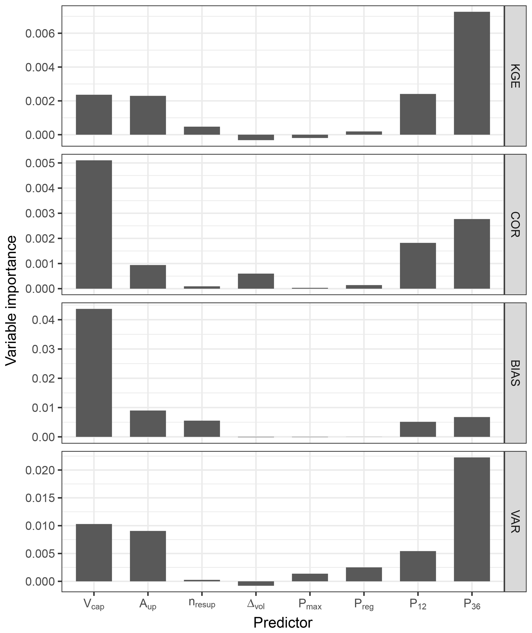
Figure 8Predictor importances for each response variable determined by the random forest approach. In this case conditional permutation importance was used (see Sect. 3.4.3).

Download

To analyse the specific influence of predictors on the response variables, Fig. 9 relates the values of the most influential predictors to the corresponding performance measures. This is done by plotting the occurrences of predictor categories in the highest and smallest valued leaf nodes of all regression trees within the random forest. It shows that under dry preconditions (P₃₆=min) there is a tendency for underestimation of standard deviations (VAR=min), i.e. a less variable reservoir storage series than observed, but a better a better overall performance (KGE=max). On the other hand, under wet conditions, especially for larger upstream catchments (A_up=high), results tend to show an overestimation of variability (VAR=max), whereas under dry conditions in small catchments variability is more often underestimated. For small reservoirs correlation is mostly low. It should be noted, however, that relationships cannot always be clearly distinguished. For instance, a low precipitation sum over the preceding year (P₁₂) may result in both a high and a low KGE value, whereas very low precipitation over the preceding 3 years (P₃₆) only led to a high KGE. Furthermore, there is no relationship between reservoir capacity and KGE.

Figure 9Relative distribution of predictor class occurrences within the largest and smallest valued leaf nodes aggregated over all regression trees of the random forest for each response variable. Shown are only the most important predictors.

Download

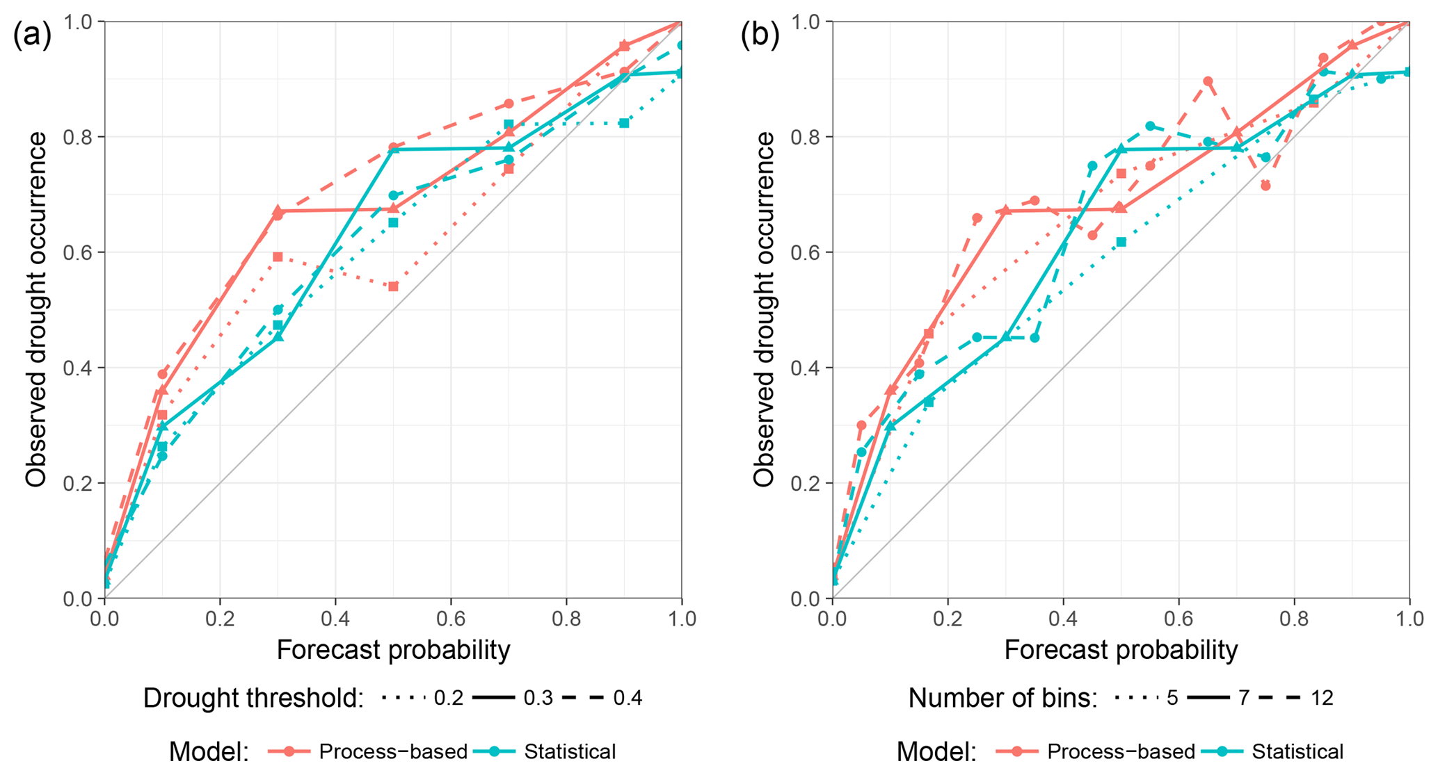
Figure 10Reliability plots for different settings of (a) drought thresholds and (b) number of probability bins. Solid lines refer to the values used in this study. The gray 1:1 lines in each plot illustrate perfect reliability for comparison.

Download

5.1 Robustness of performance metrics

There are two important algorithmic parameters affecting drought predictions of this study. One is the threshold of drought definition, i.e. the quantile of drought index observations specifying a drought, which was set to 0.3 as commonly used in the study area among water managers. This choice affects the performance values of BSS and ROCSS. The other is the number of probability bins into which hindcasts are grouped for further analysis, affecting ROCSS but not BSS as BS was herein calculated without probability binning (see Eq. 6). Figure 10 illustrates the sensitivity of verification attributes to the two parameters. It shows that a higher drought threshold results in a more evenly running curve while a smaller threshold of 0.2 tends to be better oriented towards the reliability line and appears more variable (Fig. 10a). This might result from the necessarily lower number of values of smaller thresholds. However, altogether general conclusions remain untouched, namely underforecasting and the statistical being superior to the process-based model. Regarding the number of probability bins (Fig. 10b), a larger value leads to a more variable curve. This effect can be attributed to the decreasing number of values per bin with increasing number of bins. For this study, it was decided to use a value of seven as it appears to be the best compromise between sufficient data availability per bin and an adequate number of bins for further calculations (namely ROCSS). Even affecting the values of ROCSS and partly BSS (not shown), it can be concluded that the somewhat arbitrary decision on a certain drought threshold and the number of bins, as long as reasonable values are chosen, does not affect the general results of the analysis.

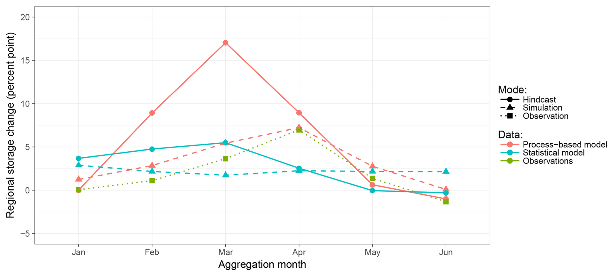
Figure 11Monthly changes of regional reservoir storage averaged over all regions, years, and hindcast members for the two models and application modes in comparison to observations.

Download

The RMSE as an accuracy measure is free of such decision parameters but is admittedly influenced in a different way. With the target variable (relative regional reservoir filling) ranging from 0 % to 100 %, the actual maximum value of the metric tends to be smaller during wet periods: the observed value (which is usually greater than zero) effectively causes the RMSE to be limited to about 40 % to 50 %. This effect is reflected as the apparent performance plateau for the process-based model in Fig. 6 and is also likely to affect the results presented in Fig. 7. The effect that, when driven by hindcasts, the process-based model exhibits larger errors under dry than under wet conditions can be at least partially attributed to this issue. In contrast, when models are driven by observations, it seems reasonable that model simulation performance is generally better under dry conditions (Fig. 7). However, as no threshold effects can be observed and the RMSE values are always considerably lower for the statistical model, this effect should not influence general conclusions of the model comparison.

5.2 Model comparison

In terms of simulation accuracy when driven by observations and for drought event prediction in the hindcast mode, both models perform equally well. Hindcast accuracy, however, is substantially lower for the process-based approach. This result is well in line with findings of other studies that simple statistical model approaches often perform equally well or even better than complex process-based prediction systems, especially in tropical regions due to exploitable correlations among meteorological and hydrological variables (Block and Rajagopalan, 2009; Hastenrath, 2012; Sittichok et al., 2018). It has to be noted, however, that the process-based approach with the WASA-SED model achieved acceptable results on monthly (hindcasts) and even daily (calibration metrics) timescales whereas former studies in NEB reported passable results only aggregated over seasonal scales (Galvão et al., 2005; Block et al., 2009; Alves et al., 2012).

The reason for the discrepancy of model ranking between simulation and hindcast mode can be attributed to the different model structures. To illustrate this, Fig. 11 shows the average monthly changes of regional reservoir storage for the different models and modes in comparison to observations. For the simulation mode (dashed lines) it can be seen that the process-based model, though exhibiting a constant overestimation, all in all is well in line with observations. The statistical model, however, shows a more or less constant storage change over the whole simulation horizon, resulting in over- and underestimations and, eventually, a good overall simulation performance (see Fig. 3). In hindcast mode (solid lines), for the process-based model the overestimation of storage change is much more pronounced and the peak shifted from April to March. Although the statistical model now more realistically exhibits seasonal dynamics, the general pattern still appears too smooth, which effectively results in less deviation from observations than the output of the process-based model (Fig. 4). This indicates a strong influence of precipitation forcing on the process-based model while the statistical approach shows less pronounced reactions to changes in the rainfall input. Consequently, deficiencies in this forcing affect the process-based model much more. This, in addition to the plateau effect discussed in Sect. 5.1, explains the more diverse RMSE values among the hindcast realisations for the process-based model at the beginning of the rainy season when reservoirs are filling up (Fig. 6) and the higher RMSE under antecedent dry conditions (Fig. 7 middle and right panels). In contrast, for the statistical model, the general patterns of RMSE over different lead times or under different antecedent moisture conditions do not change in hindcast mode when compared to simulation mode. The issue of uncertainties arising from defective precipitation forcing will be discussed in more detail later on.

Despite the lower prediction performance, the process-based approach still provides benefits over the statistical model. This includes the potential access and investigation of multiple spatially distributed hydrological variables with daily resolution, such as evapotranspiration, runoff generation, or streamflow, which were generated during the model runs. This clearly excels over the statistical model, which only yielded predictions of a single target variable. Another advantage is that model output is not only provided in a regionally and monthly aggregated manner, as for the statistical approach, but for all individual strategic reservoirs in the area as daily time series. Figure 12 illustrates that accuracies of individual reservoirs exhibit a slightly larger variation, but the RMSEs of individual reservoirs are at a similar level as when regionally aggregated. This suggests that most of the single reservoirs can be modelled with a comparable performance to the regionally aggregated values.

A further advantage of a model such as WASA-SED is that underlying processes are directly represented. As such it can be of higher value to water managers interested not only in streamflow or reservoir level forecasts but also in the investigation of process behaviour or assessments under changing boundary conditions. Therein the model could be used in scenario analyses, such as climate change impact assessment, or sensitivity analyses of, for instance, uncertain meteorological input to detect critical streamflow or reservoir stages. Furthermore, the model is transferable and can be easily applied in different regions and over different spatial and temporal scales, only limited by computational resources and available input data.

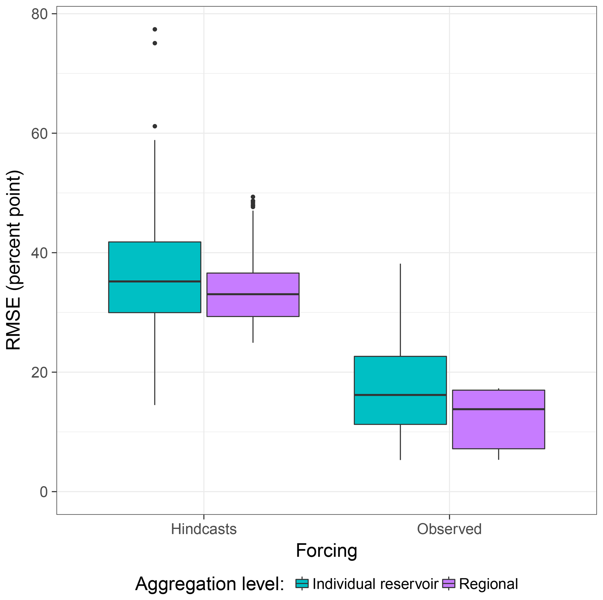
Figure 12Comparison of accuracies of the process-based model for different spatial aggregation levels on a monthly timescale.

Download

5.3 Deficiencies of the process-based simulation approach

To improve the performance of the process-based model it is first necessary to identify sources for simulation inaccuracies. It was shown that the process-based model achieved regionally different performances. A comparison of Fig. 3 and Table 3 reveals that regional bias during the calibration period is in compliance with the ranking of regional simulation errors. Moreover, although exhibiting the highest BE value, the region of Banabuiú is characterised by the largest bias during calibration and highest simulation and hindcast errors. As the latter is observed for both the process-based and statistical approaches, the reason is suspected to originate from uncertainties in observations, i.e. precipitation measurements within the region, or defective reservoir level acquisition. The reason for the Salgado region being out of the general pattern for the process-based model certainly originates from the different calibration procedure applied here, namely the use of streamflow measurements in contrast to reservoir dynamics as for the other regions. In addition, the region is distinct from other parts of the catchment in terms of environmental settings such as larger groundwater influence and sedimentary plateaus in the headwater area. Conversely, the transfer of the calibrated parameters from Castanhão to the Lower Jaguaribe region seems justifiable as the simulation error was small. Overall, reservoir size largely influences both simulated storage time series and bias. Model performance, however, appears to not be superior for large reservoirs. Moreover, wetness condition in terms of antecedent rainfall sums over the last 36 months is of major importance, i.e. dry conditions lead to the best model performance in terms of KGE. The latter is not surprising as rainfall in the study area is extremely heterogeneous both in space and time, usually characterised by convective heavy precipitation events with short durations. Thus, prolonged periods without rain constitute a spatially more homogenous input. Conversely, the aggregation of rainfall to daily sums and interpolation over subbasin units, on average covering an area of about 700 km², must necessarily induce uncertainties. The assimilation of observed reservoir filling states at the beginning of each hindcast season is therefore a reasonable approach to improve predictions and compensate for preceding rainfall input uncertainties during the initialisation run.

5.4 Potential improvements

There are several options to make use of the findings of this study and improve the forecast system in upcoming applications. In the presented study, observed reservoir level data were assimilated into the process-based model to correct the initial conditions for the hindcast runs by simply replacing model states by measurements. For assimilation, more formal approaches already exist, such as the rich families of Kalman and particle filtering approaches (e.g. Liu and Gupta, 2007; Komma et al., 2008; Vrugt et al., 2013; Sun et al., 2016; Yan et al., 2017). These, however, require a profound quantification of both simulation and observation uncertainties and, thus, much additional information and, moreover, significantly higher expenses in terms of data preparation, processing, and model application. Nevertheless, they hold the potential to better account for uncertainties in the observations, which were disregarded in this study, despite being considerable.

Preprocessing schemes in the context of hydrological forecasting usually focus on the improvement of rainfall predictions used as main drivers for hydrological models (e.g. Kelly and Krzysztofowicz, 2000; Reggiani and Weerts, 2008; Verkade et al., 2013). This is partly already included in the downscaling scheme applied to GCM products but may as well be further extended. The importance of rainfall forcing on model results, especially for the process-based approach, was already addressed above. A further comparison of the statistical properties (distribution of daily sums, dry/wet spell lengths) of rainfall hindcasts used in this study with observations revealed large discrepancies. Some preliminary tests suggested these to be responsible for the decreased accuracy of the process-based model hindcasts (not shown). In comparison to observations, the hindcasts contain (i) a general shift of rainfall seasonality towards the first months of the rainy season; (ii) a much lower frequency of both wet and dry periods for spell lengths up to 4 days; (iii) a lower frequency of low daily rainfall values while the number of large precipitation events is overestimated and daily extreme values are much higher; and (iv) a much higher probability that a dry day follows a dry day, and the probability that a wet day follows a wet day is often underestimated. These findings indicate a high potential for improvement in future applications in the study area. As a first starting point, monthly bias of hindcasts per region was corrected and both models were rerun. Figure 13 shows that this relatively simple procedure already results in a considerable decrease in RMSE for the process-based model, even though it is still higher than for the statistical approach. The improvement of drought forecast performance in terms of BSS and ROCSS is thereby less pronounced than the increase in accuracy. For the statistical model, performance metrics hardly change, which can be attributed to the smoothing effects of its model structure on regional reservoir storage identified in a previous subsection (Fig. 11).

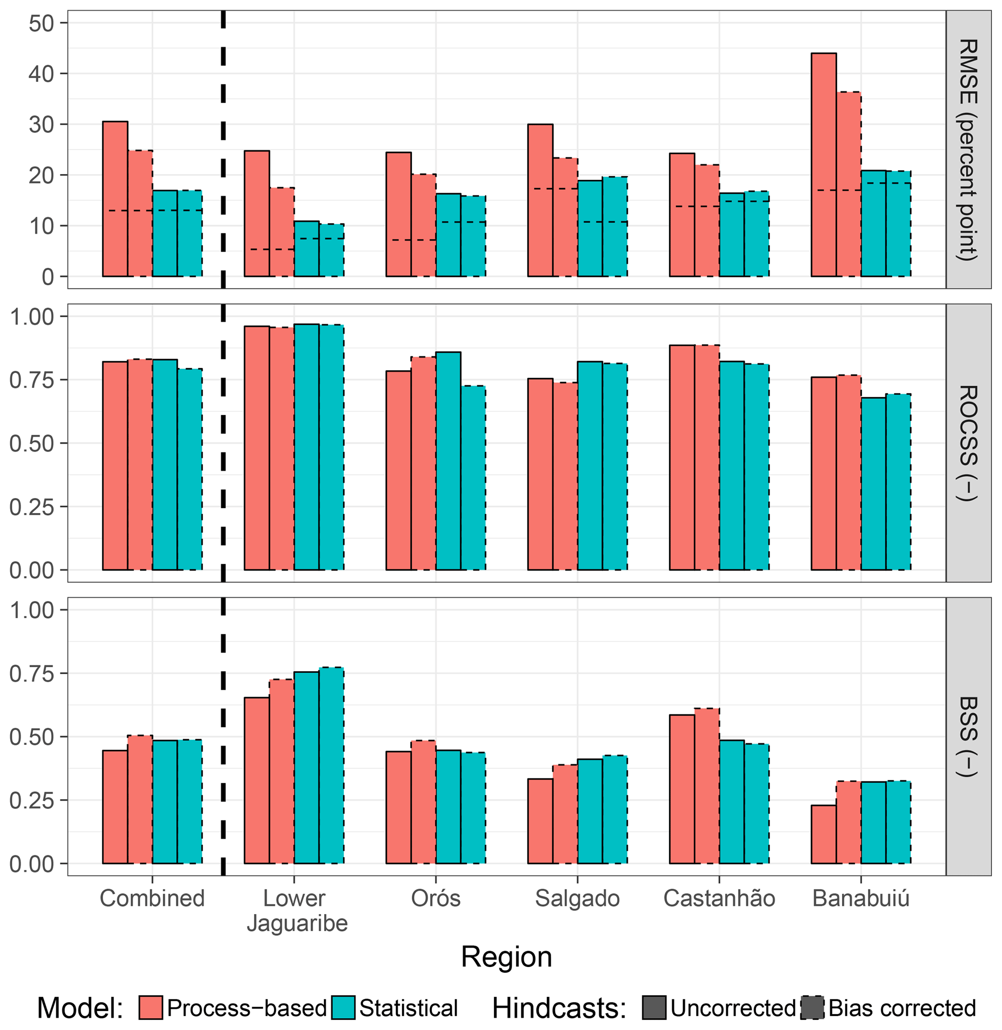
Figure 13As Fig. 4 but driving hindcasts with additional bias correction of precipitation on the monthly scale (dotted boxes).

Download

In addition to preprocessing, post-processing approaches directly tackle the correction of streamflow forecasts by statistical means including bias correction or the estimation of an error model applied to predictions (e.g. Krzysztofowicz and Kelly, 2000; Todini, 2008; Bourdin et al., 2014; Roulin and Vannitsem, 2014). Especially when focussing on extreme events, such as floods or droughts, the adequate characterisation of model residuals exhibits a large potential when incorporated into the correction of simulations and predictions (Farmer and Vogel, 2016). While being still an active field of research, such means are routinely applied in operational streamflow forecasting and, in addition to rainfall correction, could further improve model performance.

The parametrisation of the process-based model could be further improved by the use of more and different data sources. This includes, for instance, the use of satellite data to infer spatially distributed reservoir information with greater detail and more accuracy than currently available. The study area has already been of interest in ongoing research (Delgado et al., 2018a) and past studies (Heine et al., 2014) addressing that issue. In addition, management plans as well as data on water abstraction and reallocation from the larger reservoir should be included in the model but were not available for the present study. Another opportunity is to increase rainfall input resolution in the model to better account for sub-daily and spatially heterogeneous precipitation. This could be done by improving the current spatial scaling of rainfall in the model to account for heterogeneous patterns and to make use of radar rainfall data recently made available in the area.

The combination of multiple models may provide further benefits in cases where different models show strengths in different aspects of performance (e.g. Block and Rajagopalan, 2009; Schepen and Wang, 2015). However, within this work the two employed model approaches, with respect to simulation performance, achieved almost equal results and did not diverge in aspects such as lead time and antecedent moisture conditions. Thus, the combination of the two models analysed in this study is not expected to provide benefits.

5.5 Generally valid features and broader implications of results

The possibilities to generalise and transfer insights gained for one particular environment and a specific hydro-climatological setting will always be limited to questions of transferability of model approaches and the applicability of particular methods. In other word, one cannot expect that the actual numbers of model performance, be it statistical or process-based, have similar values under differing conditions. Adapting the two forecast setups presented here to other regions will presumably not lead to the same ranking of the statistical vs. the process-based model approach. In order to achieve an optimal forecast score, it is obvious that the forecast design, e.g. selection of target variables, models, and input data, needs to be tailored to the region of interest and to the purpose of the forecast including the designated forecast lead time. The design of the statistical forecast approach presented here is particularly tailored to the rather specific hydro-climatological and landscape conditions of this semiarid region. In our case, the statistical model relies on antecedent wetness conditions of the basin, quantified by precipitation indices (SPI and SPEI) aggregated over several months (see regression equations in Table 2). This satisfactorily describes the attenuated hydrological behaviour of this particular semiarid region, which is further influenced by many large and small reservoirs, in order to obtain forecasts over several months. This adaptation to the regional peculiarities does not per se allow a spatial transfer of the derived statistical model. However, the application of the underlying statistical model principles to other regions is generally possible, given that appropriate regional information and forcing data are available.

The transfer of a process-based hydrological model to another region is, generally speaking, more straight forward, because one can rely on the fact that the underlying physical assumptions and process descriptions of the model are valid for different environments and hydro-climatological conditions. In other words, the hydrological model implicitly contains the representation of general hydrological processes and, therefore, represents an adequate working hypothesis of the hydrological system at other target locations. Still, process-based models also require a sufficient data availability and quality at the region of interest while forecast performance for both model types primarily depends on the quality of rainfall forecasts.

The question of which modelling approach will finally yield a better performance score cannot universally be answered. On the one hand, this is dependent on the predictive power (i.e. the strength of correlation between predictors and target variable) of the statistical model and, on the other hand, on the validity of the physical assumptions and governing equations of the process-based model. Both model strategies benefit from good data conditions, while the required type of data is rather different. The advantage of a statistical model approach as presented here is that less distributed data of the catchment are required and the model is easier to establish and needs much less computational power. On the other hand, the process-based model allows us to simulate a rather large variety of hydrological variables in a spatially distributed manner. This enables independent verification of process-based models and leads further to a high explanatory power of this model type, which are important advantages, even for cases where the overall performance of a process-based model might be lower compared to a statistical model approach.