the Creative Commons Attribution 4.0 License.
the Creative Commons Attribution 4.0 License.
 | 15 Apr 2019
Assessment of precipitation error propagation in multi-model global water resource reanalysis
Md Abul Ehsan Bhuiyan
Efthymios I. Nikolopoulos
Emmanouil N. Anagnostou
Jan Polcher
Clément Albergel
Emanuel Dutra
Gabriel Fink
Alberto Martínez-de la Torre
Simon Munier
This study focuses on the Iberian Peninsula and investigates the propagation of precipitation uncertainty, and its interaction with hydrologic modeling, in global water resource reanalysis. Analysis is based on ensemble hydrologic simulations for a period spanning 11 years (2000–2010). To simulate the hydrological variables of surface runoff, subsurface runoff, and evapotranspiration, we used four land surface models (LSMs) – JULES (Joint UK Land Environment Simulator), ORCHIDEE (Organising Carbon and Hydrology In Dynamic Ecosystems), SURFEX (Surface Externalisée), and HTESSEL (Hydrology – Tiled European Centre for Medium-Range Weather Forecasts – ECMWF – Scheme for Surface Exchanges over Land) – and one global hydrological model, WaterGAP3 (Water – a Global Assessment and Prognosis). Simulations were carried out for five precipitation products – CMORPH (the Climate Prediction Center Morphing technique of the National Oceanic and Atmospheric Administration, or NOAA), PERSIANN (Precipitation Estimation from Remotely Sensed Information using Artificial Neural Networks), 3B42V(7), ECMWF reanalysis, and a machine-learning-based blended product. As a reference, we used a ground-based observation-driven precipitation dataset, named SAFRAN, available at 5 km, 1 h resolution. We present relative performances of hydrologic variables for the different multi-model and multi-forcing scenarios. Overall, results reveal the complexity of the interaction between precipitation characteristics and different modeling schemes and show that uncertainties in the model simulations are attributed to both uncertainty in precipitation forcing and the model structure. Surface runoff is strongly sensitive to precipitation uncertainty, and the degree of sensitivity depends significantly on the runoff generation scheme of each model examined. Evapotranspiration fluxes are comparatively less sensitive for this study region. Finally, our results suggest that there is no single model–forcing combination that can outperform all others consistently for all variables examined and thus reinforce the fact that there are significant benefits to exploring different model structures as part of the overall modeling approaches used for water resource applications.


Improved estimation of global precipitation is important to the analysis of continental water resources and dynamics. Over the past few decades, several studies have described the use of different precipitation algorithms to develop precipitation products (http://ipwg.isac.cnr.it/algorithms.html, last access: 31 March 2019 and http://reanalyses.org, last access: 31 March 2019) at high spatial and temporal resolution on a quasi-global scale and for different hydrological applications, such as flood early warning and control and drought monitoring (Hong et al., 2010; Wu et al., 2012; Vernimmen et al., 2012, amongst others). Precipitation estimates suffer, however, from various sources of error that consequently impact hydrologic investigations (Mei et al., 2015, 2016; Seyyedi et al., 2014, 2015; Bhuiyan et al., 2017; Nikolopoulos et al., 2013).
Over the last decade, an increasing number of studies have contributed to the development of global precipitation estimation (Pan et al., 2010; Beck et al., 2017a; Kirstetter et al., 2014; Carr et al., 2015; Dee et al., 2011) aiming at the overall improvement of the hydrological applications and global water resource reanalysis. Numerous models of varying complexity can be used to generate an array of hydrological products from precipitation forcing datasets (Vivoni et al., 2007; Ogden and Julien, 1994; Carpenter et al., 2001; Borga, 2002; Schellekens et al., 2017). Different hydrological models have different applications depending on the spatial and temporal scales of interest as well as the simulated variables of interest, such as subsurface runoff, surface runoff, and evapotranspiration. Past studies (Fekete et al., 2004; Biemans et al., 2009) have revealed that the uncertainty in simulated hydrological variables mainly depends on the uncertainty in precipitation and model parametrization and suggested subsequent exploration of different model structures as part of the overall modeling approach.
So far there are several studies that have analyzed uncertainty in precipitation forcing and its impact on hydrologic simulations by usually evaluating hydrologic simulations based on multiple forcing applied to a single model (Falck et al., 2015; Bitew et al., 2012; Behrangi et al., 2011; Mei et al., 2016; Bhuiyan et al., 2018; Gelati et al., 2018 among others). On the other hand, there are also past studies that have evaluated the model structural uncertainty and its impact on hydrologic simulations, usually by analyzing the simulation outputs from multiple models and a single forcing dataset (Breuer et al., 2009; Haddeland et al., 2011; Gudmundsson et al., 2012; Smith et al., 2013; Huang et al., 2017; Beck et al., 2017b). However, fewer studies have been dedicated to the analysis of the integrated impact of both forcing and model uncertainty on hydrologic simulations, and from the existing ones, most of them were focused on a single hydrologic variable such as streamflow (see, for example, Qi et al. 2016), evapotranspiration (Vinukollu et al., 2011), or a given hydrologic index such as the drought index (Prudhomme et al., 2014; Samaniego et al., 2017). Findings from these past investigations have demonstrated that both forcing and model structure uncertainty have a great impact on hydrologic predictions and therefore highlight that using a multi-model and multi-forcing ensemble is a more appropriate path forward for advancing the use of hydrologic model outputs. This conclusion raises at the same time the need for better understanding, characterizing and quantifying the uncertainty associated with multi-model and multi-forcing hydrologic ensembles. Thus, a better understanding of the ensemble spread of precipitation and simulated hydrological variables is necessary to improve water resource management and planning. This additionally means that there is also a need to assess hydrologic uncertainty in more than a single variable to be able to have a better and more integrative view on the interaction between forcing uncertainty, model uncertainty, and the hydrologic variable of interest. It will allow us to make hydrologic predictions more effective for water resource applications at a large scale.
This study builds upon a unique numerical experiment that was carried out, as part of the activities of the Earth2Observe project (Schellekens et al., 2017), to investigate the impact of precipitation uncertainty propagation and its dependence on model structure and hydrologic variables. In this investigation, we used different precipitation forcing datasets based on (i) reanalysis, (ii) satellite estimates, and (iii) a “combined” stochastic precipitation dataset (Bhuiyan et al., 2018). To consider model structure and parameters, we examined simulations from five state-of-the-art global-scale hydrological and land surface models (LSMs). With regard to water cycle variables, we evaluated precipitation uncertainty propagation to surface runoff, subsurface runoff, and evapotranspiration fluxes. The study area for this investigation is the Iberian Peninsula, which has precipitation and climate variability due to complex orography influenced by both Atlantic and Mediterranean climates (Rodríguez-Puebla et al., 2001; de Luis et al., 2010; Herrera et al., 2012). The analysis comprised two main parts: (1) performance and sensitivity evaluation of the different model–forcing scenarios and (2) precipitation uncertainty propagation to the hydrological variables. We analyzed hydrological simulation with a comparative assessment of the hydrological products and provided a detailed analysis of uncertainty in hydrological simulations for the different global hydrological and land surface models used in the multi-model global water resource reanalysis. Finally, we examined the performance of precipitation products in hydrological applications and potential uncertainty attributed to precipitation error propagations.
The paper is structured as follows. Section 2 presents the different types of forcing datasets used for the study, and Sect. 3 details the methodology we used for our model development and hydrological model analysis. Section 4 summarizes the hydrological results, Sect. 5 discusses the results, and Sect. 6 draws conclusions from the research conducted.
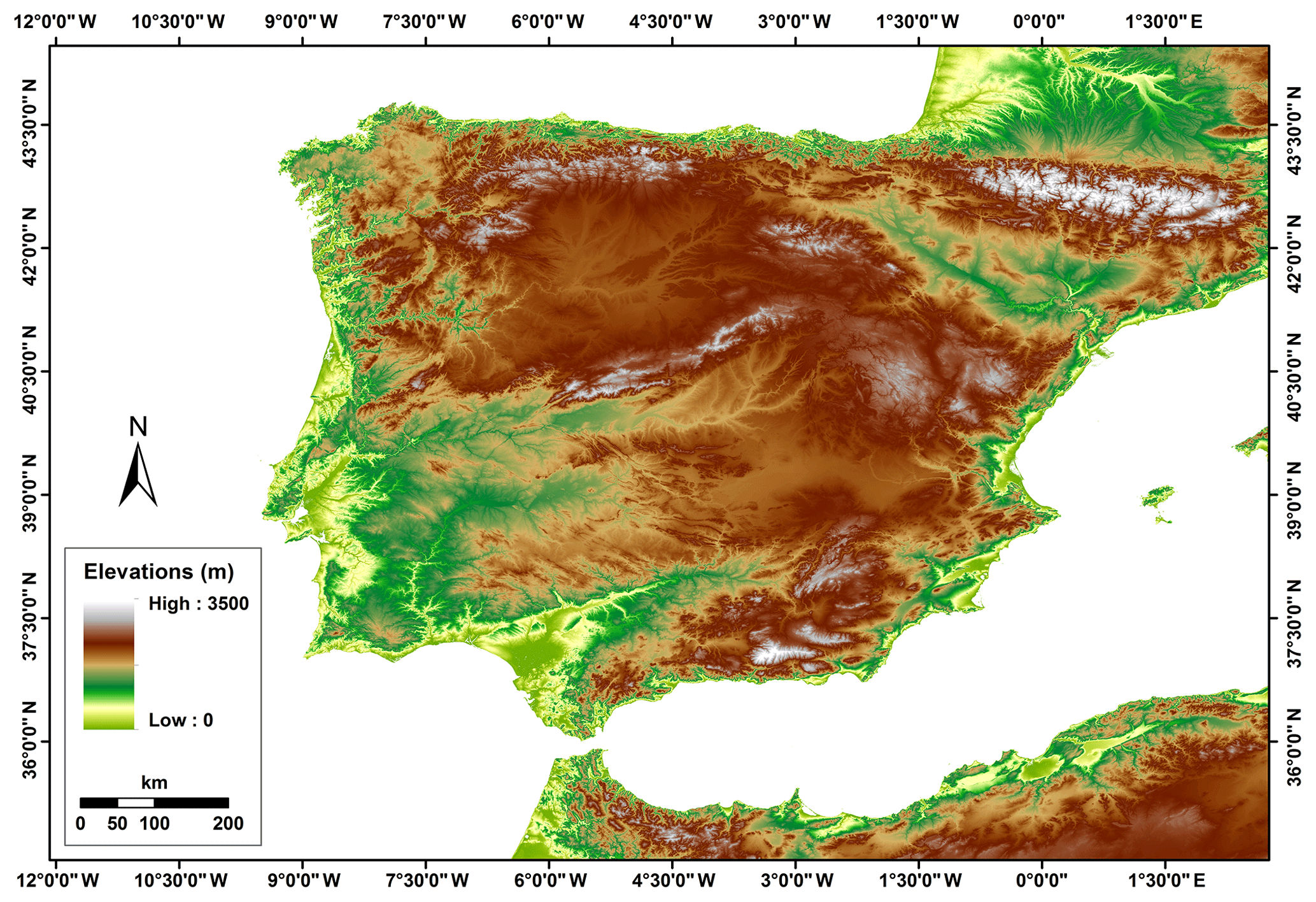
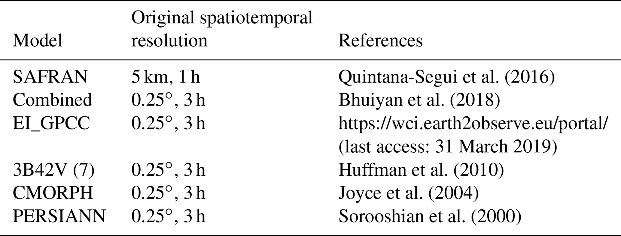
This study is focused on the Iberian Peninsula (Fig. 1). The climate of the peninsula is primarily Mediterranean, being mostly oceanic at northern and semi-arid at southern parts. The topography varies from almost zero elevation to altitudes of 3500 m in the Pyrenees. Table 1 summarizes information and references of meteorological forcing datasets, and a short description is provided below.
2.1 Reference precipitation (SAFRAN)
The reference precipitation dataset, hereafter referred to as SAFRAN (Système d'analyse fournissant des renseignements atmosphériques à la neige), was recently created by Quintana-Seguí et al. (2016, 2017) using the SAFRAN meteorological analysis system (Durand et al., 1993). Spatially, SAFRAN precipitation data are presented at an hourly timescale on a regular grid with 5 km resolution, spanning 35 years and covering mainland Spain, Portugal, and the Balearic Islands (Quintana-Seguí et al., 2016). SAFRAN used an optimal interpolation algorithm (Gandin, 1966) to produce a quality-controlled gridded dataset of precipitation which combines ground observations and outputs of a meteorological model (Quintana-Seguí et al., 2017). Quintana-Seguí et al. (2017) also compared the different precipitation analyses with rain gauge data and successfully evaluated their temporal and spatial similarities to the observations by obtaining higher correlation (>0.75) than other precipitation products. The validation of SAFRAN with independent ground observations proved that SAFRAN is a robust product. On the other hand, several factors – including rainfall intermittency, discrete temporal sampling, and censoring of reference values for required quality – reduce the number of comparison samples for reference and satellite estimates. Therefore, the quality-controlled SAFRAN dataset which is designed to force the land surface model is chosen as a reference dataset for the study area (Quintana-Seguí et al., 2017).
2.2 Satellite-based precipitation
Satellite-based simulations were based on three quasi-global satellite precipitation products. Among them, CMORPH (the Climate Prediction Center Morphing technique of the National Oceanic and Atmospheric Administration, or NOAA) is developed from passive microwave (PMW) satellite precipitation fields which are generated from motion vectors derived from infrared (IR) data (Joyce et al., 2004). A neural network technique is used in PERSIANN (Precipitation Estimation from Remotely Sensed Information using Artificial Neural Networks), where IR observations are connected to PMW rainfall estimates (Sorooshian et al., 2000). Merged IR and PMW precipitation products from NASA are gauge-adjusted for TMPA (Tropical Rainfall Measuring Mission Multi-Satellite Precipitation Analysis), or 3B42V(7), which is available in near-real time and post-real time (Huffman et al., 2010). The satellite precipitation products have a spatial resolution that is 0.25∘ × 0.25∘ and a time resolution of 3 h.
2.3 Atmospheric reanalysis
The reanalysis product (EI_GPCC) is based on original ERA-Interim 3-hourly data, after rescaling based on GPCC (Global Precipitation Climatology Center) data. Note that total precipitation has been rescaled at the monthly scale with a multiplicative factor to match GPCC version 7 for the period 1979–2013 and GPCC monitoring for 2013–2015. Data are further downscaled to 0.25∘ × 0.25∘ grid resolution by distributing the coarse grid precipitation according to CHPclim (Climate Hazards Group Precipitation Climatology) high-resolution information for each calendar month. A similar approach was performed in the generation of ERA-Interim/Land (Balsamo et al., 2015), but using GPCP (Global Precipitation Climatology Project) data. In this study we used GPCC data due to its higher spatial resolution when compared with GPCP.
2.4 Combined product
The combined product is based on the application of a nonparametric statistical technique for blending multiple satellite–reanalysis precipitation datasets. Specifically, a machine-learning technique, quantile regression forests (QRF; Meinshausen, 2006), was used to generate stochastically an improved precipitation ensemble at the spatiotemporal resolution of 0.25∘, 3 h. The technique optimally merged global precipitation datasets and characterized the uncertainty of the combined product. Details on the methodology and data used to develop the combined product are presented in Bhuiyan et al. (2018).
2.5 Other atmospheric variables
Apart from precipitation forcing, the rest of atmospheric forcing variables required for the hydrologic simulations were derived from the original ERA-Interim 3-hourly data as used in ERA-Interim/Land (Balsamo et al., 2015), bilinearly interpolated to 0.25∘. It includes a topographic adjustment to temperature, humidity, and pressure using a spatially temporally varying environmental lapse rate (ELR) computed similarly to Gao et al. (2012). The correction is the following: (i) relative humidity is computed from the uncorrected forcing, (ii) air temperature is corrected using the ELR and altitude differences (ERA-Interim topography versus 0.25 topography), (iii) surface pressure is corrected assuming the altitude difference and updated temperature, and (iv) specific humidity is computed using the new surface pressure and temperature assuming no changes in relative humidity.
3.1 Hydrological simulations
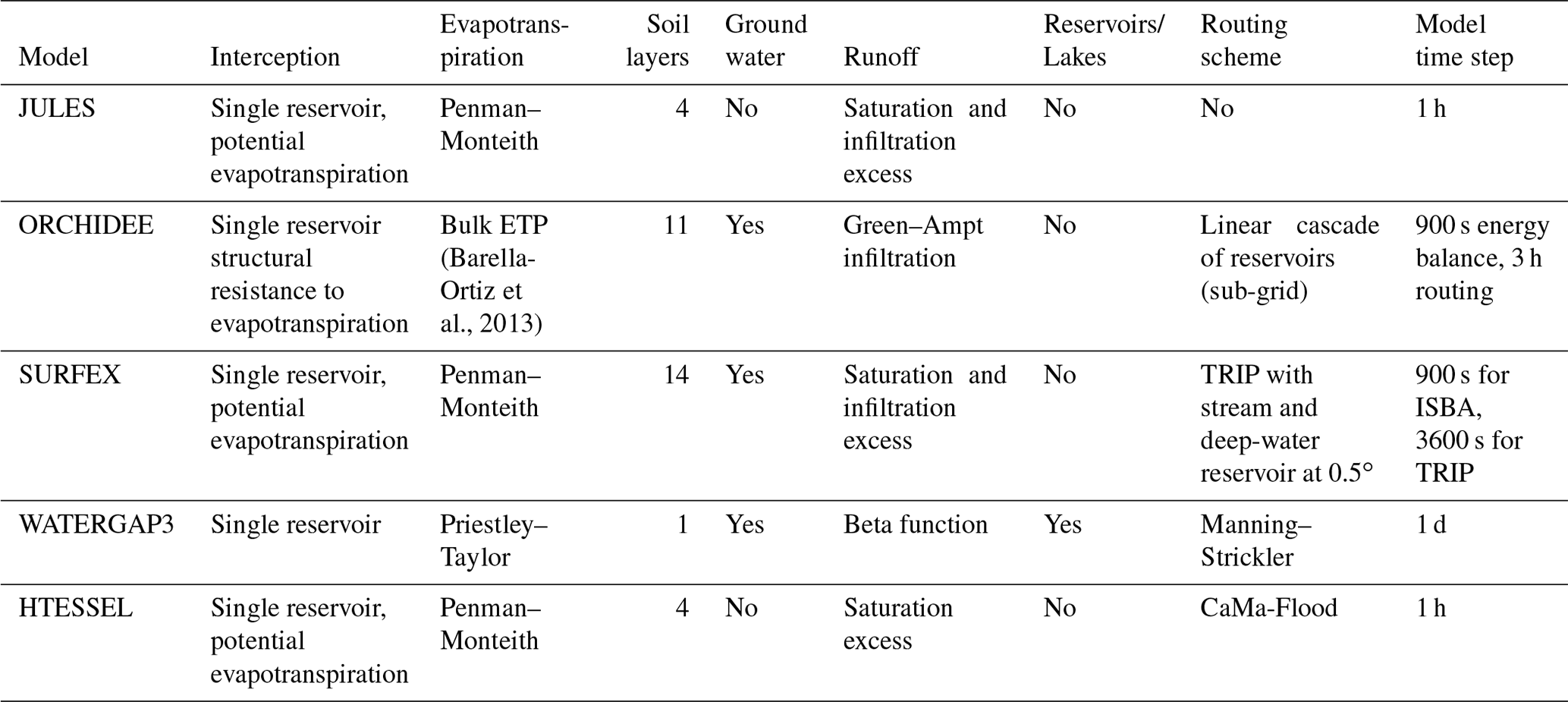
The hydrological simulations for this study were carried out by different collaborators within the framework of Earth2Observe, a project funded by the European Union (EU) using a number of global-scale land surface and hydrological models. In this study, simulations from four land surface models – JULES (Joint UK Land Environment Simulator), ORCHIDEE (Organising Carbon and Hydrology In Dynamic Ecosystems), SURFEX (Surface Externalisée), and HTESSEL (Hydrology – Tiled European Centre for Medium-Range Weather Forecasts – ECMWF – Scheme for Surface Exchanges over Land) – and one global hydrological model, the distributed global hydrological model of the WaterGAP3 (Water – a Global Assessment and Prognosis) modeling framework were considered. The models were already evaluated at all timescales, from daily to multi-annual. The timescale of the evaluation was mostly driven by the data availability. All the land surface models in the study were global models, built originally to work in coupled mode with atmospheric models. The “regionalization”, or calibration of hydrological parameters at particular catchments or regions of these models, is an exercise that the different modeling groups or communities are certainly performing but was out of the scope of this study. All models were forced with the various precipitation datasets described in the previous section for an 11-year period (March 2000–December 2010). A summary of some basic characteristics of the models structure is presented in Table 1 and a short description is provided below. For more details on the modeling systems, the interested reader is referred to Schellekens et al. (2017) and references therein.
3.1.1 JULES
JULES (Best et al., 2011; Clark et al., 2011) is a physically based land surface model. JULES uses an exponential rainfall intensity distribution to calculate throughfall through the canopy first (altered by interception), then the water reaching the surface is divided into infiltration into the soil and surface runoff. Surface runoff is generated either through infiltration excess or saturation excess. Infiltration excess runoff is generated by JULES if the water flux reaching the surface exceeds the maximum infiltration rate of the soil (based on the saturated hydraulic conductivity). If the water flux reaching the surface over a time step (either rainfall, throughfall, or snowmelt) reaches a maximal infiltration rate, then infiltration excess runoff will be generated. This maximal infiltration rate in JULES is the saturated hydraulic conductivity multiplied by a vegetation-dependent parameter (four for trees and two for grasses). Saturation excess runoff is based on sub-grid soil moisture variability, as a fraction of the grid is saturated and water flux over this fraction is converted to surface runoff (probability distribution model; Blyth, 2002). Once infiltrated into the soil, water flows through the column, resolved using Darcy's law and Richards' equation. Subsurface runoff is calculated using the free drainage approach, with water flowing at the bottom of the resolved soil column at a rate determined by the soil hydraulic conductivity. There was no groundwater table in this version of JULES. The condition at the bottom of the resolved soil layers (3 m) was assumed to be free drainage. The soil hydraulic characteristics were calculated applying pedotransfer functions to the soil texture data from the Harmonized World Soil Database (HWSD; FAO/IIASA/ISRIC/ISS-CAS/JRC, 2012).The vegetation cover data used by the JULES runs were derived from the International Geosphere-Biosphere Programme at http://www.igbp.net/ (last access: 31 March 2019). Further details on hydrology processes in JULES can be found in Best et al. (2011) and Blyth et al. (2018).
3.1.2 ORCHIDEE
ORCHIDEE (Krinner et al., 2005) is a complex land surface scheme that consists of a hydrological module, a routing module (Ngo-Duc et al., 2007), and a floodplain module (d'Orgeval et al., 2008). It also describes the vegetation dynamics and biological cycles, but these features were not activated for the present study. The most relevant parametrization of ORCHIDEE for the sensitivity of the model to rainfall is the one for partitioning between infiltration and surface runoff. In order to represent correctly the fast progression of the moisture front during a rainfall event when the time step is above 15 min, a time-splitting procedure is used (d'Orgeval, 2006). The parametrization also takes into account reinfiltration in the case of slopes below 0.5 % or dense vegetation. We have chosen to spread the entire 3-hourly rainfall over 1.5 h in these simulations. In terms of ancillary data, a vegetation map (IGBP; Olson classification) and the soil types (FAO, 2003) were used for these simulations. Furthermore, as ORCHIDEE represents sub-grid soil moisture by simulating separately the soil moisture column below bare soil, low and high vegetation, the infiltration process will display different sensitivities in each column.
3.1.3 SURFEX
The SURFEX modeling system of Météo-France (SURFace Externalisée; Masson et al., 2013) includes the ISBA (interactions between soil–biosphere–atmosphere; Noilhan and Mahfouf, 1996) LSM that can be fully coupled to the CNRM (Centre National de Recherches Météorologiques) version of the Total Runoff Integrating Pathways (TRIPs; Oki and Sud, 1998) continental hydrological system (Decharme et al., 2010). This study uses a ISBA multi-layer soil diffusion scheme (ISBA-Dif) as well as its 12-layer explicit snow scheme (Boone and Etchevers, 2001; Decharme et al., 2016). ISBA total runoff is contributed by both the surface runoff and free drainage as a bottom boundary condition soil layer. The soil evaporation is proportional to its relative humidity. Parameters of the ISBA LSM were defined for 12 generic land surface patches: nine plant functional types (namely needleleaf trees, evergreen broadleaf trees, deciduous broadleaf trees, C3 crops, C4 crops, C4 irrigated crops, herbaceous plants, tropical herbaceous plants, and wetlands) as well as bare soil, rocks, and permanent snow and ice surfaces. They were derived from ECOCLIMAP-II, the land cover map used in SURFEX (Faroux et al., 2013). Furthermore, the Dunne runoff (i.e., when no further soil moisture storage is available) and lateral subsurface flow were computed using a topographic sub-grid distribution.
3.1.4 WATERGAP3
The modeling framework WaterGAP3 is a tool for assessing the global freshwater resources on 30 min spatial resolution. It combines a spatially distributed rainfall–runoff model with a large-scale water quality model as well as models for five sectorial water uses (Flörke et al., 2013; Döll et al., 2009). Effective precipitation – calculated as superposed effects of snow accumulation, snowmelt, and interception – is split into (i) a fraction that fills up a single-layer soil moisture storage and (ii) a fraction that comprises surface runoff and groundwater recharge. Groundwater recharge is the input of a single linear groundwater reservoir that is drained by base flow. Water for evapotranspiration, estimated with the Priestley–Taylor approach, is abstracted from the soil storage. The WaterGAP3 setting used in this study was calibrated and validated against measured river discharge from 2446 stations of the Global Runoff Data Centre data repository (Weedon et al., 2014). Therefore, calibration only concerns the separation of effective precipitation into runoff and soil moisture filling. See Eisner (2015) for a detailed model description with additional data required for the model, such as soil types and the groundwater table.
3.1.5 HTESSEL
The LSM HTESSEL is part of the ECMWF numerical weather prediction model. The model represents the temporal evolution of the snowpack, soil moisture and temperature, and vegetation water content as well as the turbulent exchanges of water and energy with the atmosphere. HTESSEL considered soil texture, vegetation type and cover, and mean annual climatology of the leaf area index and albedo (12 maps for each calendar year) for the simulations (FAO, 2003). The soil column is discretized in four layers (7, 21, 72, and 189 cm thickness), and the unsaturated vertical movement of water follows Richards' equation and Darcy's law. The van Genuchten formulation is used to derive the diffusivity and hydraulic conductivity using six predefined soil textures. In the case of partially or fully frozen soil, the water movement in the soil column is limited by reducing the diffusivity and hydraulic conductivity. The model assumes free drainage as a bottom boundary condition (subsurface runoff), while the top boundary condition considers precipitation minus surface runoff and bare ground evaporation. Evapotranspiration is removed from the different soil layers following a prescribed root distribution (dependent on the vegetation type). Surface runoff generation is estimated as a function of the local orography variability, soil moisture state, and rainfall intensity. Soil saturation state and rainfall intensity define the maximum infiltration rate which is modulated by a variable infiltration rate related to orography variability (Balsamo et al., 2009).
3.2 Evaluation metrics
To examine the magnitude and variability of differences among hydrological variables, we used the relative difference (RD), defined as
where yi denotes reference variables (SAFRAN-driven simulations) and denotes simulated variables (based on the other forcing data considered) for each time step i. RD indicates the magnitude and direction of error with positive (negative) value indicating overestimation (underestimation). The RD of annual average estimates of the precipitation forcing and different hydrological variables was calculated using daily datasets at the spatial resolution of 0.25∘. Moreover, cumulative probability of estimated annual average relative differences among precipitation forcings and the simulated hydrological variables were calculated using same spatial resolutions of 0.25∘.
To collectively assess the performance of various precipitation forcing datasets, models, and simulated hydrological variables, we used a normalized version of the Taylor diagram (Taylor, 2001). Specifically, we normalized the values of the centered root-mean-square error (CRMSE) and the standard deviation with the standard deviation of the reference. Therefore, the reference (that is, the target point to which the model outputs should be closest) corresponds to the point on the graph with the normalized CRMSE equal to zero, while both the correlation coefficient and normalized standard deviation equal 1. The normalized Taylor diagrams summarized model results for two different temporal scales (3-hourly and daily) at the spatial resolution of 0.25∘.
To evaluate the degree of variation of various precipitation datasets and simulated hydrological variables, we used the coefficient of variation (CV) and coefficient of variation ratio (CVr). The CV and CVr are determined using all precipitation forcing and variables examined at the 0.25∘ daily resolution. The CV is a measure of variability defined as the ratio of the standard deviation to the mean. To compare the degree of variation from one data series to another, we used the CV where we considered distributions with CV<1 to be low variance, while we considered those with CV>1 to be high variance. We defined CVr as the ratio of the CV of model to the CV of reference. The defined parameters are expressed as follows:
The CVm and CVo indicate the coefficient of variation of the model and the coefficient of variation of reference, with the means and and standard deviations σm and σo, respectively. The CVr includes two components: the ratio of the means and ratio of the standard deviation. Details on the statistical metrics, including name conventions and mathematical formulas, are provided in the Appendix.
3.3 Metrics of uncertainty propagation
The random error component was based on the normalized centered root-mean-square error (NCRMSE). To demonstrate how error in precipitation forcing translates to error in the simulated hydrological variables – surface runoff (Qs), subsurface runoff (Qsb), and evapotranspiration (ET) – we used the NCRMSE error metric ratio as follows:
where NCRMSE is the normalized centered root-mean-square error and αNCRMSE is NCRMSE error metric ratio at multiple temporal (3-hourly and daily) and spatial (0.25∘) resolutions. The αNCRMSE metric quantifies the changes in the random error from precipitation to simulated hydrological variables (Qs, Qsb, and ET) and can thus be used to assess magnification (αNCRMSE>1) or damping (αNCRMSE<1).
3.4 Analysis of ensemble spread
To assess how variability in the precipitation ensemble translates to variability of the various hydrological simulations (Qs, Qsb, and ET) for the different modeling systems, we performed an analysis of ensemble spread (Δ), formulated as
in which Xmax and Xmin represent, respectively, the maximum and minimum of ensemble values at each time step, while Y is the corresponding value of the reference. Here, the members of ensemble constitute a sequence for each time step . The ensemble spread (Δ) is calculated at the monthly scale for the combined product and simulated hydrologic variables. Note that the combined product is an ensemble-based precipitation product; for the evaluations presented in this study, we use the ensemble mean as forcing. For the analysis and propagation of the precipitation ensemble spread to hydrologic simulations, we used 20 ensemble members, which are generated stochastically by the QRF tree-based regression model (Meinshausen, 2006). Δ provides a measurement of the expected prediction intervals relative to the reference value. The Δ value of 1 indicates the maximum possible uncertainty of the prediction interval. To achieve accurate and successful prediction, comparatively small prediction intervals are expected.
4.1 Variability of multiple hydrological model simulations
To examine the magnitude and variability of the differences among both models and forcing datasets, we analyzed the multi-model simulation results for three hydrological variables, including surface runoff (Qs), subsurface runoff (Qsb), and evapotranspiration (ET). Throughout this analysis, we used the SAFRAN-based simulation as the reference for comparison. Figures 2 to 5 present spatial maps of annual average values for each model, along with the relative differences of annual average estimates of precipitation forcing and the different hydrological variables for all the precipitation forcing datasets and models. The relative differences in precipitation forcing (Fig. 2) exhibited considerable spatial variability for satellite precipitation forcing (relative difference >20 %) and relatively lower variability for EI_GPCC and the combined product. Examination of SAFRAN-based annual average values of surface runoff shows that WaterGAP3 estimates considerably higher surface runoff than the rest of the models, particularly in the northern and northwestern part of the study area (Fig. 3). Consequently, subsurface runoff (Fig. 4) and evapotranspiration (Fig. 5) from WaterGAP3 were lower in that part of the study area. All these results display substantial differences in the spatial pattern of relative differences, which suggests that simulations are sensitive to both precipitation forcing and model uncertainty. Certain models seem to be more sensitive for given variables. For example, HTESSEL and ORCHIDEE are the models with the largest relative difference of Qs, and both models exhibited different behaviour relative to the other models when forced by the satellite precipitation. This suggests a distinct structural difference in the way precipitation is partitioned into surface–subsurface runoff between the two groups.
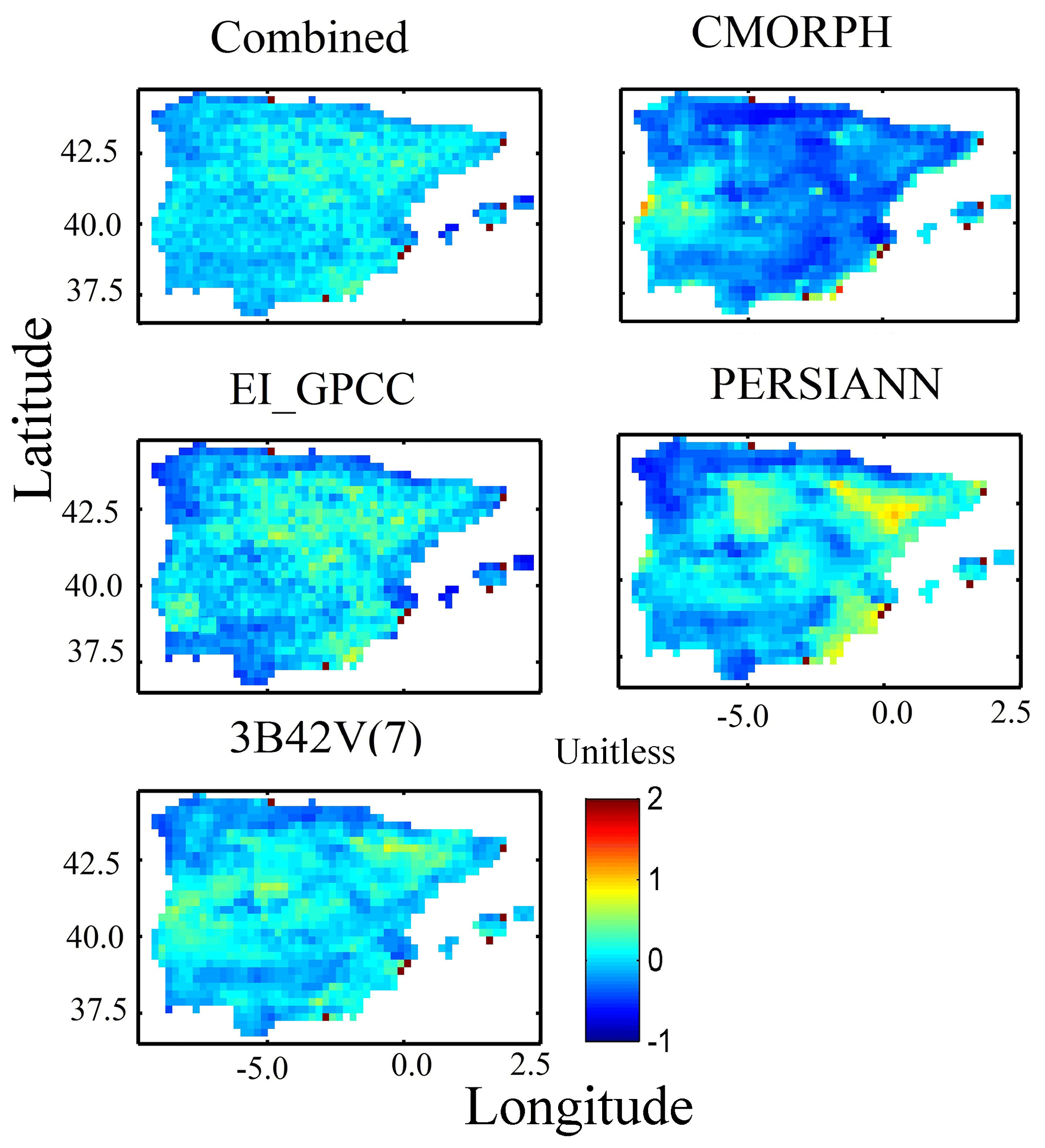
Figure 2Map of the annual average relative difference (with respect to SAFRAN) for the different precipitation forcing datasets.
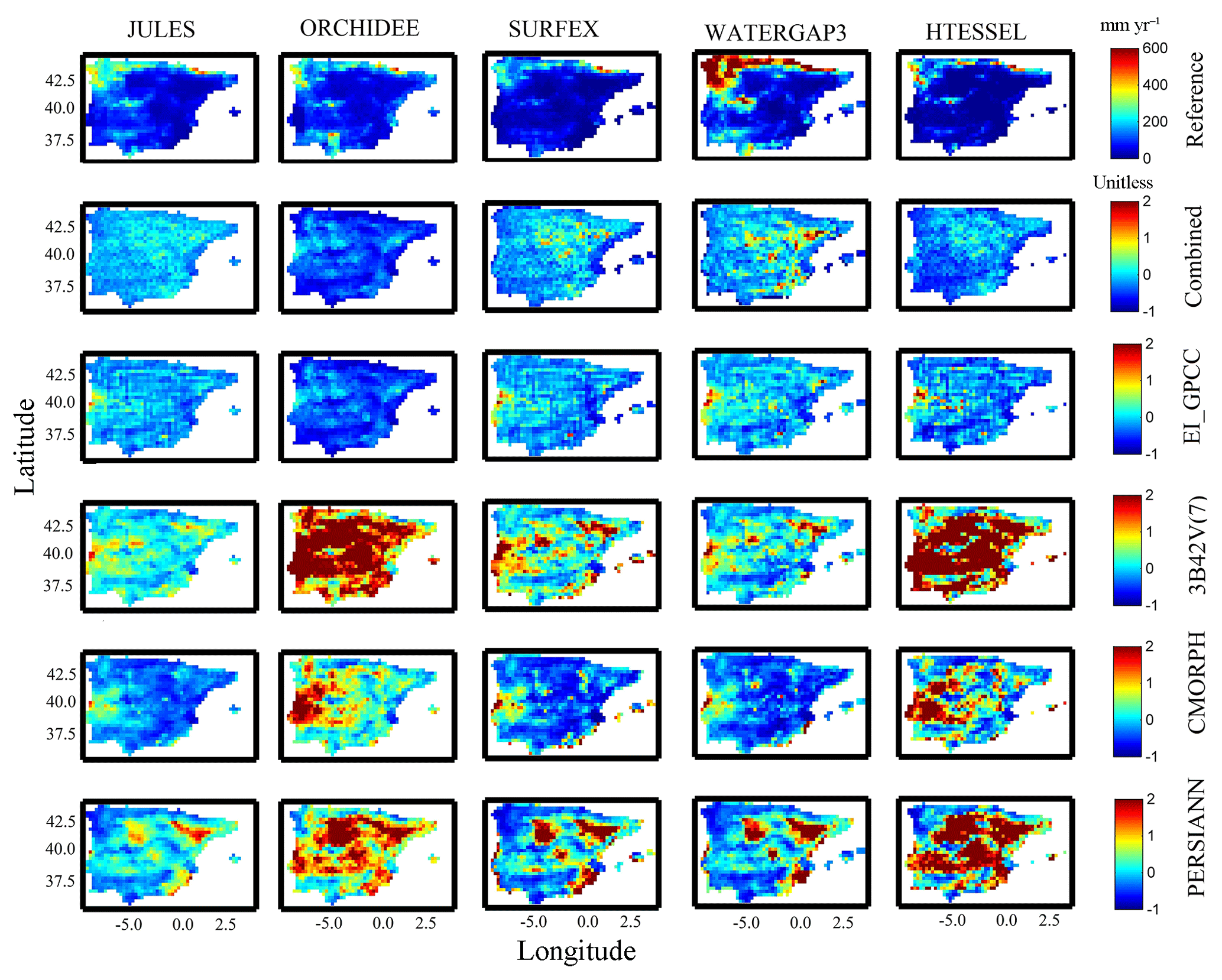
Figure 3Map of SAFRAN-based simulations (Reference) of surface runoff (top row), and relative difference for the various models (columns) and precipitation forcing (rows 2–5) analyzed.
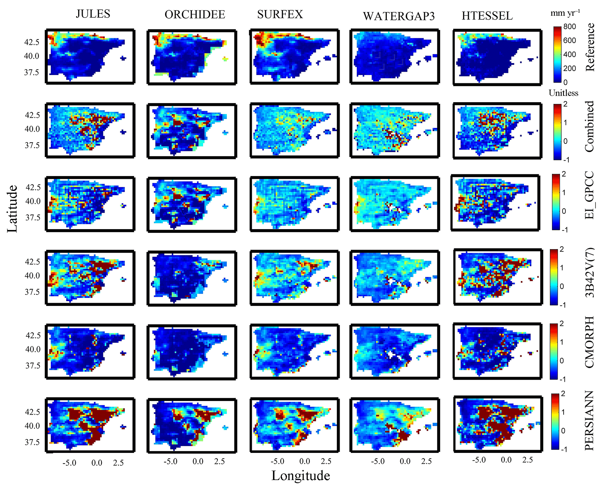
Figure 4Map of SAFRAN-based simulations (Reference) of subsurface runoff (top row), and relative difference for the various models (columns) and precipitation forcing (rows 2–5) analyzed.
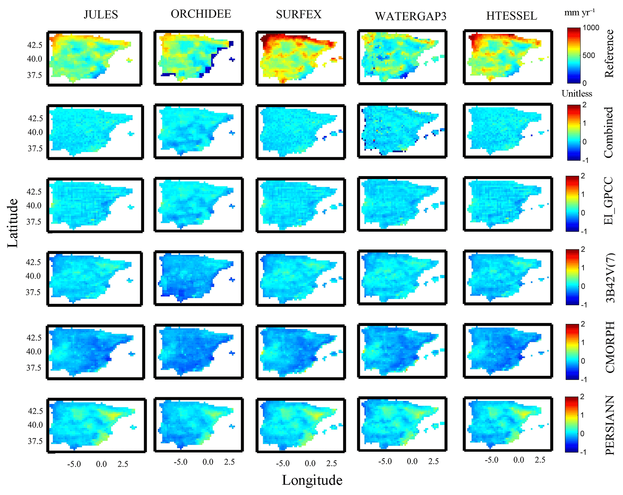
Figure 5Map of SAFRAN-based simulations (Reference) of evapotranspiration (top row), and relative difference for the various models (columns) and precipitation forcing (rows 2–5) analyzed.
Looking at the variability of results for combined and reanalysis (EI_GPCC) forcing datasets, no substantial differences occurred between reference and simulated surface runoff (Qs). However, for the satellite-based simulations, there were significant deviations. Specifically, the CMORPH-based simulation showed significant overestimation for ORCHIDEE and HTESSEL, but this pattern was reversed for JULES, SURFEX, and WaterGAP3, an outcome that highlights the impact of model structure on precipitation error propagation.
For subsurface runoff, similar spatial patterns (with respect to Qs) were exhibited for the reference and the rest of simulations (Fig. 4), which were also affected substantially by precipitation uncertainty. For example, looking at the different model simulations, we can see that WaterGAP3 results reveal the lowest relative differences in Qs for almost all the precipitation forcings. In addition, CMORPH-based simulation underestimated substantially for all the models. Figure 5 presents the spatial pattern of the results for evapotranspiration. For the combined product and EI_GPCC, results were consistent with low relative difference (<25 %). On the other hand, CMORPH-based simulation showed an overall underestimation and deviated considerably from the results of the other precipitation products. By examining the spatial pattern of relative differences (Figs. 2–5), one can recognize that there is no consistent spatial pattern among the different model–forcing combinations. There are cases where the pattern of the differences is dominated by the pattern of precipitation differences, as, for example, in the case of PERSIANN, where the maximum number of differences are concentrated in the central and eastern part of the peninsula. While there are other cases where the pattern is dominated by the sensitivity of the model (see, for example, results for ORCHIDEE and 3B42 for surface runoff).
We also present a comparison of cumulative probability of the relative differences among precipitation forcings (Fig. 6) and the simulated hydrological variables (Fig. 7). The distribution of relative differences, both in terms of type (denoted by the shape of the cumulative density function – CDF) and magnitude and differed as a function of precipitation forcing, the model, and the variable considered. The CDF of precipitation relative differences shows that CMORPH deviated significantly from the other precipitation products (Fig. 6). The surface runoff based on ORCHIDEE and HTESSEL displayed a clear separation of the CDF for the combined product and EI_GPCC and satellite-based precipitation forcing (Fig. 7). Specifically, it is interesting to note that 3B42V(7) responds very differently to other precipitation forcing datasets for ORCHIDEE, highlighting again the sensitivity of runoff response to precipitation structure (space–time variability) and its dependence on the rainfall–runoff generation mechanism.
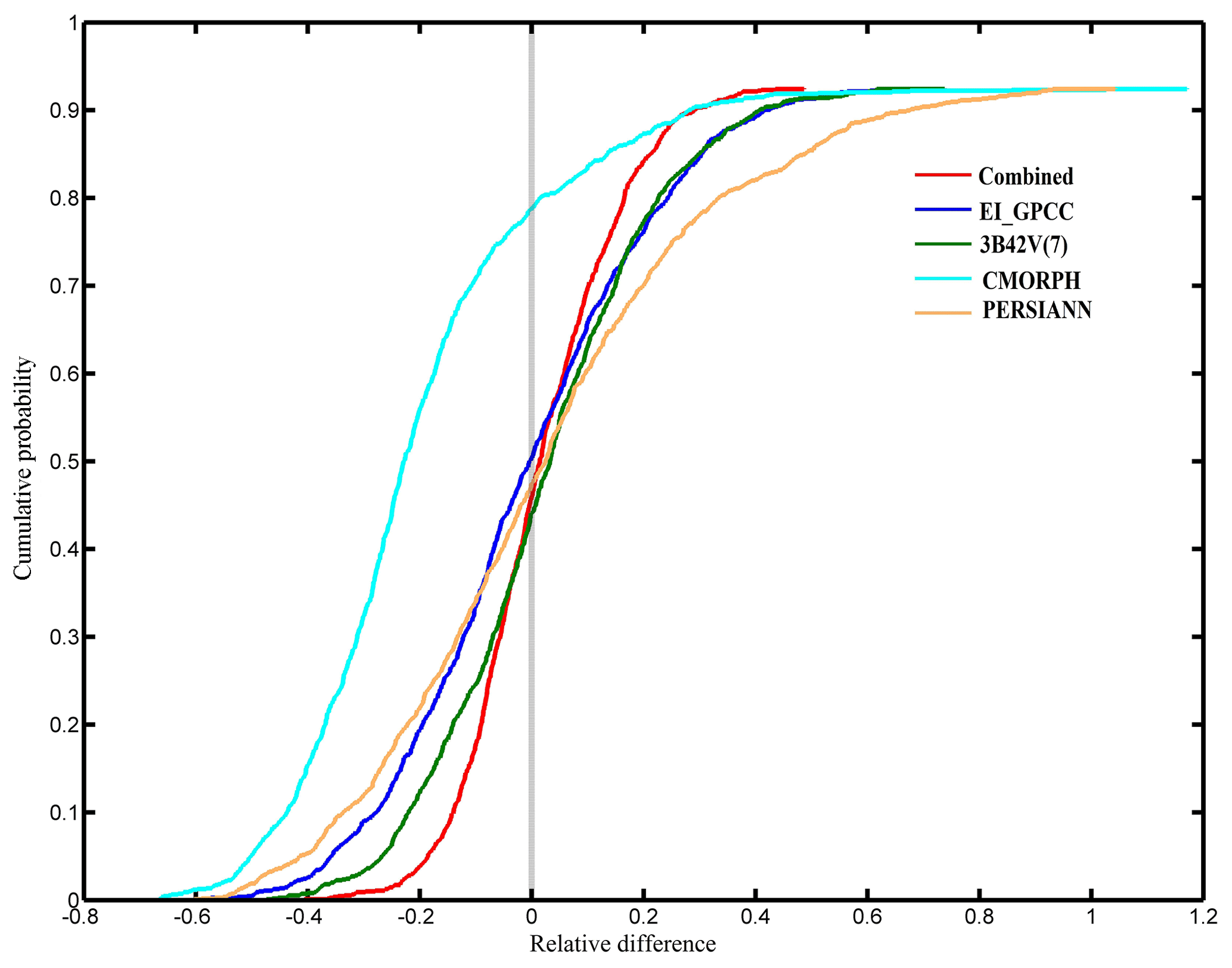
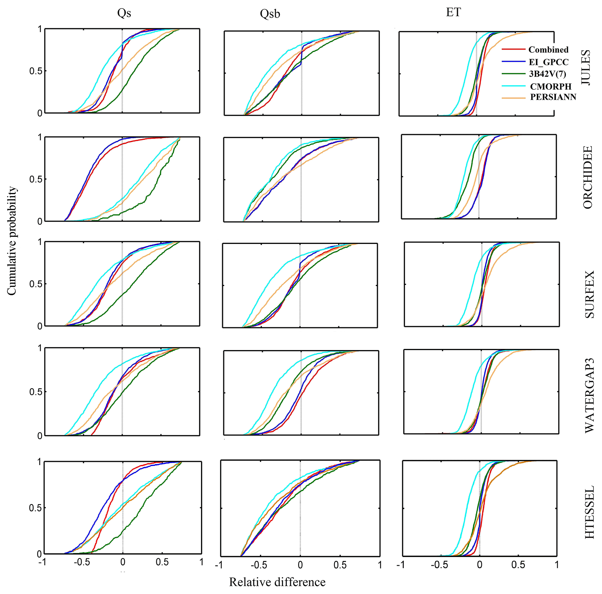
Figure 7Cumulative probability for the multi-model, multi-forcing simulations for simulated hydrological variables.
Box plots of the relative difference of different hydrological variables for the various forcing datasets and models at the daily scale are shown in Fig. 8. Note the inclusion of the relative difference of precipitation forcing to allow the comparison between relative differences in precipitation with those in the other hydrological variables. For each model, the box plot shows a lower interquartile range (IQR), marking lower variability for Qsb and ET compared to Qs. Results for simulations based on the combined product and EI_GPCC showed less variability than the satellite-based simulations. SURFEX and WaterGAP3 exhibited the lowest variability compared to the other models. Overall, with the exception of few cases (e.g., 3B42V(7) for ORCHIDEE and HTESSEL and CMORPH for ORCHIDEE), uncertainty reduces progressively from precipitation to surface runoff, subsurface runoff, and finally ET.
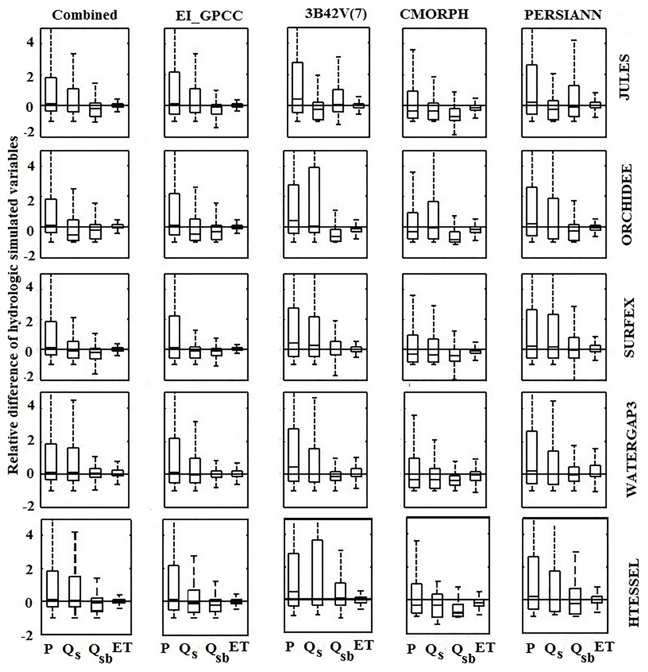
Figure 8Relative difference presented for the various products and models at daily scale. In each box, the central mark is the median, and the edges are the first and third quartiles.
4.2 Performance of multi-model simulations
The normalized Taylor diagrams summarize the results for two different temporal scales. Figure 9 shows the results for the 3-hourly scale only for the two models with output available at that resolution (JULES and SURFEX), while Fig. 10 presents results at the daily scale for all five models. We aggregated the 3-hourly results from JULES and SURFEX to daily to compare them with the nominal daily output of ORCHIDEE, WaterGAP3, and HTESSEL. Results improved with the temporal aggregation in reducing random error for JULES and SURFEX. As shown in Fig. 10, the points for the 3B42V(7) were always the furthest from the reference (NCRMSE>0.75) with the low correlation coefficient (0.4–0.55), except SURFEX, which means that 3B42V(7) was always associated with the worst performance for all other models. Simulations based on the combined product and EI_GPCC were always consistent, with significantly reduced NCRMSE values in the range of 0.25–0.8 for all the hydrological models. Results for simulated ET are more consistent among the various precipitation forcing datasets, exhibiting normalized standard deviations in the range of 0.8–1.2. NCRMSE reduced significantly (<0.35) for each forcing dataset; accordingly, the correlation coefficient (CC) also raised considerably (>0.9), showing a very high degree of agreement with reference-based simulations. For surface–subsurface runoff, the SURFEX and WaterGAP3 models performed comparatively better than other models by reducing NCRMSE values, especially for the combined product and EI_GPCC.
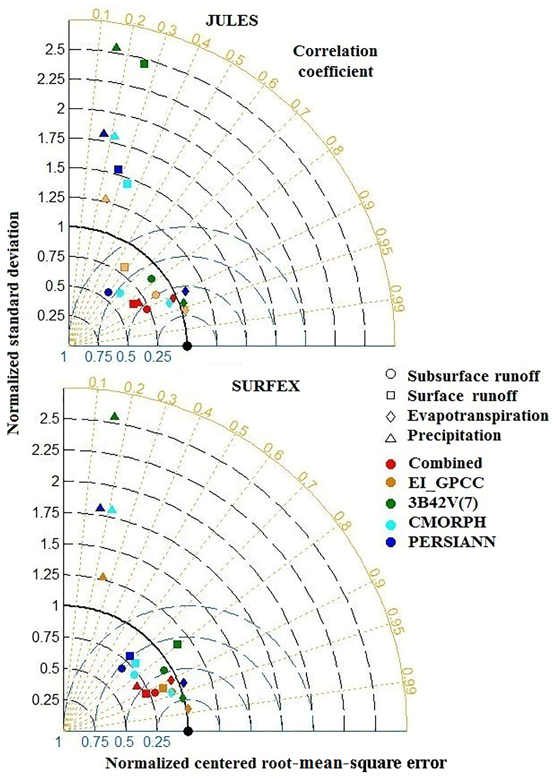
Figure 9Normalized Taylor diagrams for 3-hourly precipitation and simulated hydrological variables based on SAFRAN and the satellite–reanalysis precipitation products used.
To illustrate the relative variability between precipitation and individual hydrological variables, we calculated the coefficient of variation (CV) and the coefficient of variation ratio (CVr) for all the hydrological models. To provide an understanding of the impact of precipitation uncertainty in hydrological simulations, we produced box plots of the CV and CVr for precipitation forcing datasets and individual hydrological variables for all the models, as shown in Fig. 11. A precipitation-forcing-wise comparison indicates that the combined product and reanalysis underestimated precipitation variability more than other precipitation forcings, which affected the corresponding variability in Qs for all the models except ORCHIDEE. Although there were no significant differences in terms of variability for combined product and reanalysis-based simulations for the four models (JULES, SURFEX, WaterGAP3, and HTESSEL), substantial differences in variability between precipitation and Qs were observed for ORCHIDEE model. Satellite products overestimated precipitation variability, leading to overestimation of the variability of surface and subsurface runoff. The variability of ET was much lower than that of the other variables examined and well captured in all the simulation scenarios. From the box plots of CV from reference-based simulations, the distributions of ET showed low variability (CV<1), while the variability for all the other hydrological variables was high (CV>1). In terms of CVr, the SURFEX model performed very well by producing medians close to 1 (CVr=1 means ideal consistency) for all the precipitation forcing datasets but CMORPH.
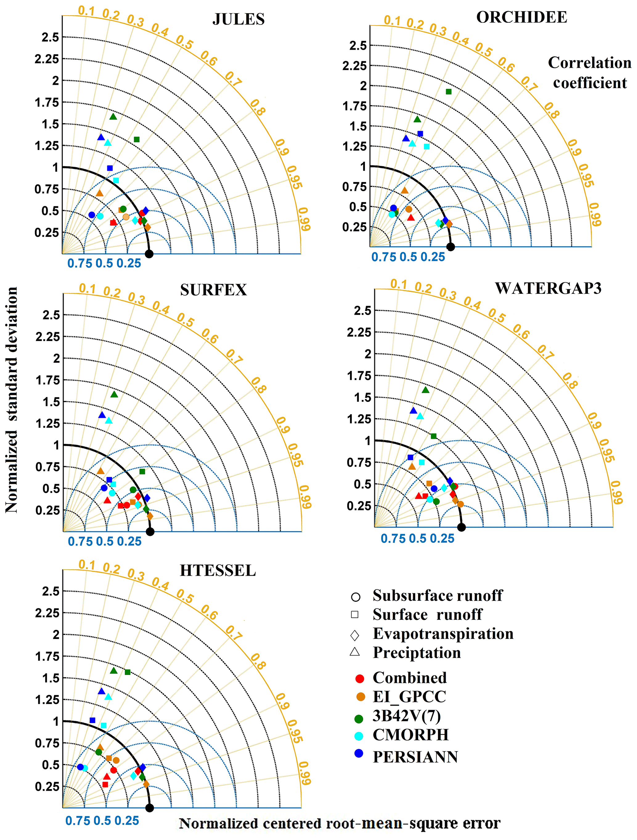
Figure 10Normalized Taylor diagrams for daily simulated hydrological variables with SAFRAN and the satellite–reanalysis precipitation products used.
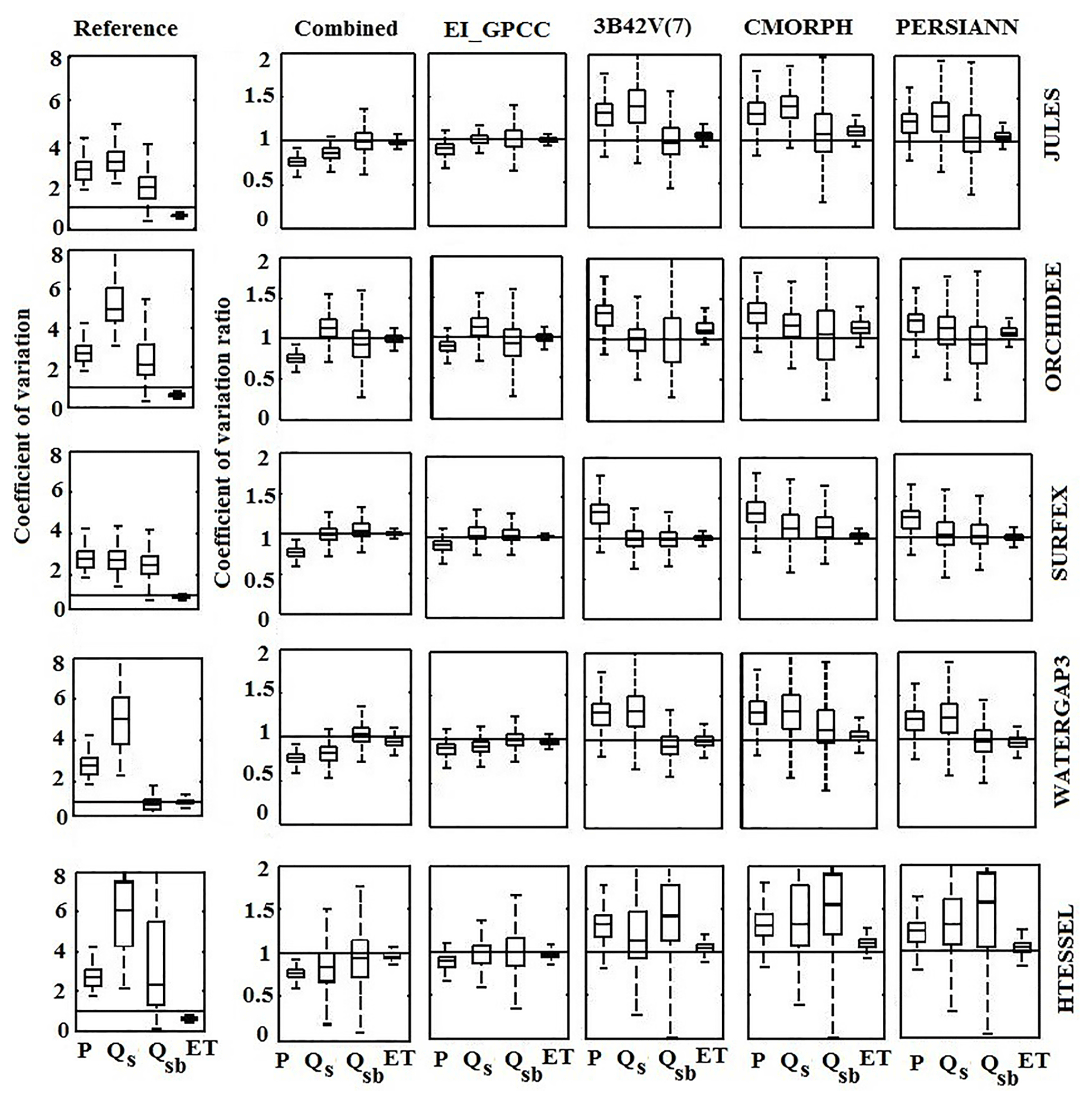
Figure 11Relationship between coefficient of variation and coefficient of variation ratio of simulated hydrological variables and precipitation.
4.3 Assessment of precipitation error propagation
To investigate the possible amplification, or dampening, of the precipitation error to the hydrologic variables examined, we quantified the NCRMSE error metric ratio (αNCRMSE), and results are illustrated in Figs. 12 and 13. For all the scenarios (at 3-hourly and daily scales) and almost all models, αNCRMSE values were less than 1, which highlighted the damping effect on the random error of precipitation in simulated variables. In general, the damping effect increases (i.e., αNCRMSE reduces), moving from surface to subsurface runoff and ET and highlighting once again the interaction between the different runoff-generating mechanisms as well as coupled water–energy balance processes and precipitation uncertainty. Interestingly, the relationship between error propagation among the different hydrologic variables varied greatly between models and precipitation forcing. Values of αNCRMSE for surface and subsurface runoff are generally close for the SURFEX model but distinctly different for satellite-based results of ORCHIDEE and WaterGAP3.
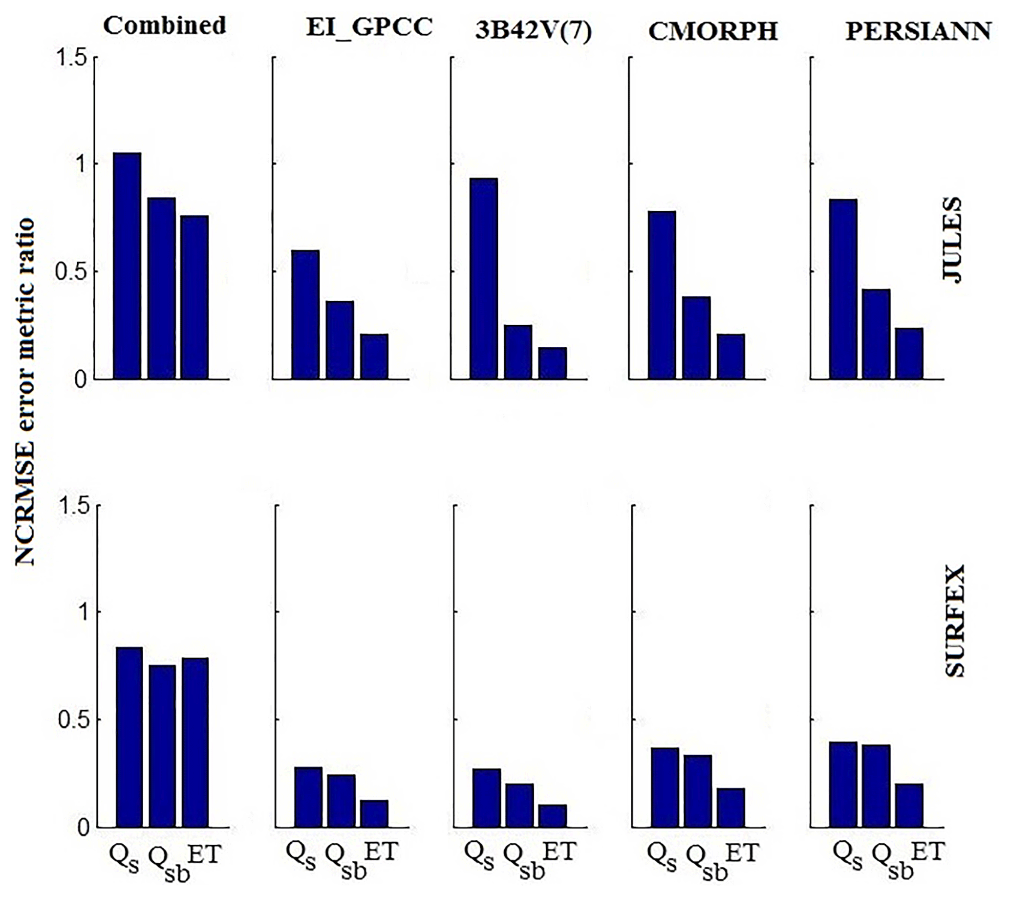
Figure 12NCRMSE error metric ratios presented for the various products and models at 3-hourly scale.
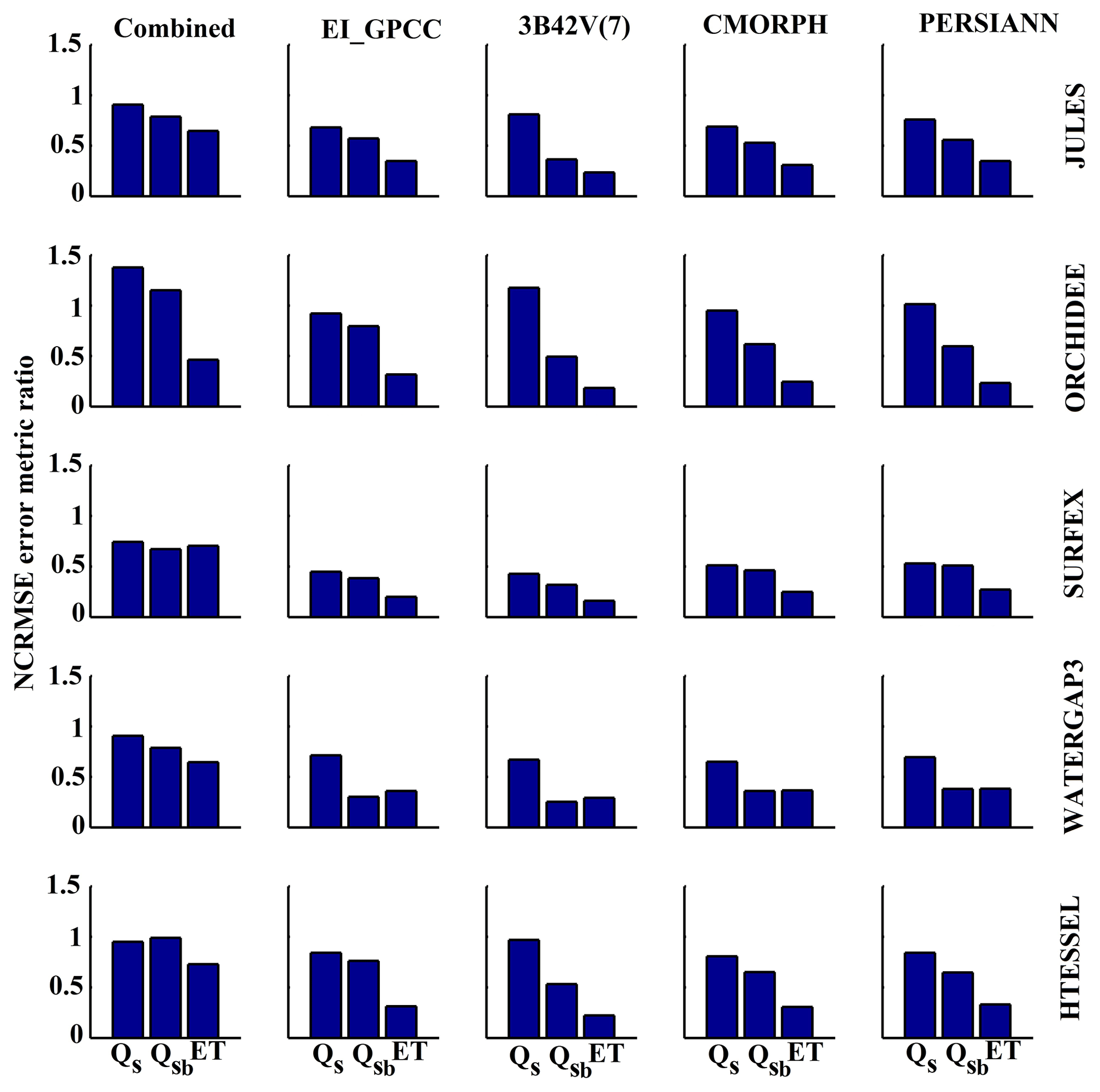
Figure 13NCRMSE error metric ratios presented for the various products and models at daily scale.
4.4 Stochastic precipitation ensemble and corresponding simulated hydrological variable analysis results
The following summarizes the results of our analysis of ensemble precipitation (20 members), generated stochastically according to the algorithm used for the combined product, and their corresponding hydrological simulations. To show the relationship between the precipitation ensemble and simulated hydrological variables (generated ensemble), we presented an analysis of ensemble spread. Figure 14 depicts density plots between ensemble spread of precipitation and the simulated hydrological variables (Qs, Qsb, and ET) at the monthly scale. A strong correlation between ensemble spread of Qs and precipitation is found for almost all models. For the other variables (ET and Qsb), ensemble spread was significantly narrower and rather independent of the ensemble spread of precipitation, manifested as the horizontal structure of contours in Fig. 14. The ensemble spread of Qs was higher (ORCHIDEE and HTESSEL) or lower (SURFEX and WaterGAP3) depending on the model, elucidating again the impact of the modeling structure on the propagation of precipitation uncertainty.
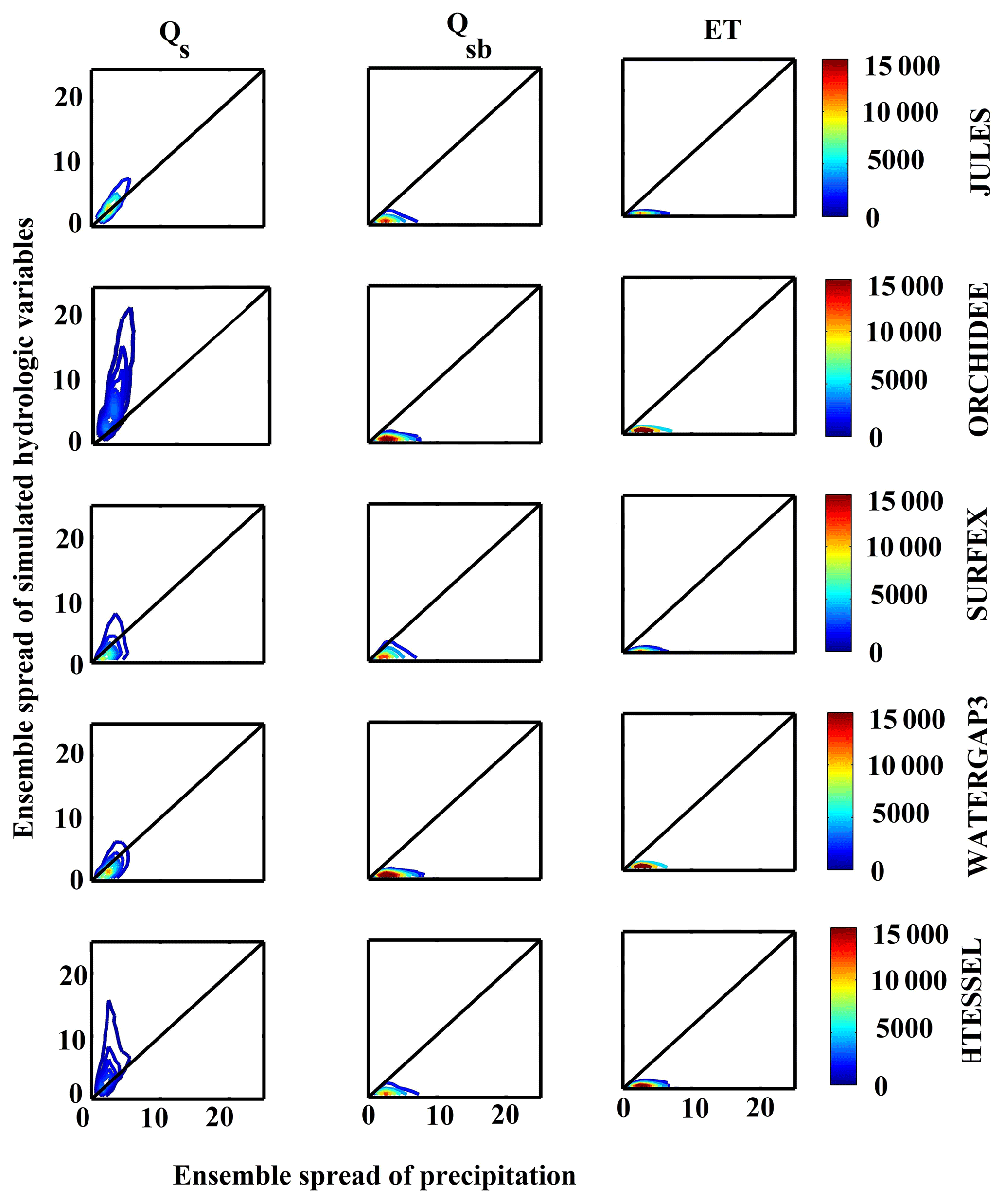
Figure 14Density contour plot of the relationship between ensemble spread of simulated hydrological variables and precipitation at monthly scale. Color scale shows the frequency of occurrence. The black line is the 1:1 line.
Precipitation from different satellite–reanalysis datasets exhibits considerable differences in pattern and magnitude, which results in significant differences in hydrologic simulations. Results presented in this paper demonstrated clearly that magnitude and dynamics of uncertainty in hydrologic simulations depend not only on the uncertainty of the forcing variable but also on the model and examined hydrologic variable.
For example, surface runoff (Qs) appears to be highly sensitive to precipitation differences, while ET was not for this semi-arid study region (Figs. 3 to 5). Particularly, ET exhibited reduced sensitivity to precipitation forcing, which potentially suggests that the water volume available for conversion to ET did not deviate significantly among the precipitation scenarios. This is expected for ET because it is primarily controlled by atmospheric demand, plant and soil hydraulic constraints, and solar radiation (Wallace and McJannet, 2010). When sufficient energy is available for rainfall to evaporate directly without contributing to surface–subsurface runoff, simulation of ET is not only affected by precipitation uncertainty but also by other atmospheric constrains.
Consequently, results (Figs. 6 to 7) for ET were more consistent among the various model and precipitation forcing scenarios, indicating a smaller degree of uncertainty in ET (relative to Qs and Qsb). These results suggest that precipitation has a stronger influence on surface runoff, in particular precipitation intensity, i.e., the same amount of precipitation distributed over 3 h or over 1 d will impact mostly surface runoff, and this is associated with the model representation of this fast process. Similarly, if we look at the distribution of precipitation relative difference, CMORPH tends to decrease in magnitude compared to other precipitation products. Therefore, for subsurface runoff, CMORPH-based simulations displayed a gross underestimation compared to other precipitation forcing.
Precipitation-to-surface-runoff sensitivity is strongly controlled by the corresponding runoff generation scheme in each model. For example, in the case of HTESSEL and ORCHIDEE, precipitation intensity has a great effect on the generation of surface runoff. The satellite precipitation datasets have higher precipitation intensities (Fig. 6) when compared to the remaining datasets, which explains the different behaviour of these two models. However, in the case of JULES, the infiltration excess mechanism is rarely invoked when the drivers are provided at a 3-hourly time step, as the maximum infiltration rate is not reached. Therefore, the significance of differences that HTESSEL and ORCHIDEE show with more intense rainfall are not shown by JULES due to distinct differences of their corresponding surface runoff generation modules.
Evaluation of the performance of the various simulations, relative to SAFRAN, emphasized the issues due to low correlation and increased random error from satellite products. On the other hand, the reanalysis (EI_GPCC) and combined product resulted in reduction of random error, suggesting that relying on gauge-adjusted reanalysis or blended (satellite–reanalysis) products offers improvement relative to satellite products alone.
Certain dynamics resolved from this analysis were generally consistent among different models, such as the fact that uncertainty reduced systematically from precipitation to surface runoff to subsurface runoff and eventually to ET simulations. This is also in accordance with our expectations, given that soil moisture (storage) integrates the precipitation variability in time. Surface runoff exhibits high correlation to precipitation, while uncertainty in subsurface runoff is modulated by storage capacity of the soils. In addition ET is affected only if water availability deviates significantly from the water demand in terms of potential evapotranspiration. Our findings related to the surface runoff uncertainty (due to model structure and precipitation) suggest that the use of surface runoff (e.g., flash floods diagnostics) should be carefully considered in each application in view of each model formulation.
This study investigated the propagation of precipitation uncertainty in hydrological simulations and its interaction with hydrologic modeling, which was based on satellite–reanalysis precipitation forcing of a number of global hydrological and land surface models for the Iberian Peninsula. The following are the major conclusions from this study.
Simulation of surface runoff was shown to be highly sensitive to precipitation forcing, but the direction (that is, overestimation or underestimation) and the magnitude of relative differences indicated strong dependence on the modeling system. Hydrological simulations based on reanalysis and combined product forcing datasets performed better overall than satellite precipitation-driven simulations. Moreover, simulation results using CMORPH as forcing exhibit overall overestimation for ORCHIDEE and HTESSEL, which is totally the opposite to the results from the other models (JULES, SURFEX, and WaterGAP3). These types of differences highlight the complexity of the interaction between precipitation characteristics and different modeling schemes and should be used as a “reference for caution” when generalizing findings produced from single model simulations.
Modeling uncertainty appeared to be much less important for evapotranspiration than for surface and subsurface runoff. The sensitivity of hydrological simulations to different precipitation forcing datasets was shown to depend on the hydrological variable use and model parameterization scheme. Finally, based on our evaluation of the performance of the different hydrological models and five precipitation products – CMORPH, PERSIANN, 3B42V(7), reanalysis, and the combined product – we could not identify a single model that consistently outperformed others, i.e., certain models appeared to be more successful in the simulation of certain variables.
This study suggests that important benefits may accrue from exploring different model structures as part of the modeling approach. This study assessed the multi-model performances regarding three different hydrologic variables (surface–subsurface runoff and evapotranspiration). Apart from precipitation forcing, other atmospheric forcing variables required for the hydrologic simulations are also essential in investigating the significance of hydrological model uncertainty. In addition, the only calibrated model in this study, WaterGAP3, performs better in specific locations (e.g., hilly) for all the hydrologic variables than other models. Therefore, investigation should be performed in calibrating and regionalizing models for different parameters. Nevertheless, a clear outcome of the current work is that uncertainty in hydrologic predictions is significant and should be assessed and quantified in order to foster the effective use of the outputs of global land surface models and hydrologic models. Considering ensemble representation (e.g., multi-model and multi-forcing) of hydrologic variables provides an appropriate path to address this issue.
Advancing our understanding of precipitation uncertainty, model uncertainty, and their interaction will potentially also aid in the investigation of the impacts of climate change (and associated uncertainty) on hydrological cycle components and water resource systems. Finally, this research provides a fine platform for discussing advances in the applications of different precipitation algorithms, hydrology, and water resource reanalysis.
The datasets are available online for SAFRAN (http://mistrals.sedoo.fr/Data-Download-IPSL/?datsId=1388&search=0&project_name=HyMeX, last access: 31 March 2019), CMORPH (ftp://ftp.cpc.ncep.noaa.gov/precip/CMORPH_V1.0/RAW/0.25deg-3HLY/, last access: 31 March 2019), PERSIANN (http://fire.eng.uci.edu/PERSIANN/data/3hrly_adj_cact_tars/, last access: 31 March 2019), 3B42V(7) (https://mirador.gsfc.nasa.gov, last access: 31 March 2019), the atmospheric reanalysis dataset (https://wci.earth2observe.eu/portal/, last access: 31 March 2019), and the combined product (https://sites.google.com/uconn.edu/ehsanbhuiyan/research, last access: 31 March 2019).
The statistical metric, the coefficient of variation ratio (CVr) used in the model evaluation analysis, was computed using the following parameters:
Here, oi and mi () are the observed and modeled time series, respectively, of the product for times i, with the means and and standard deviations σo and σm, respectively; N is the total number of data points used in the calculations.
The numerical experiments of this study were conceived during discussions of the Earth2Observe EU project. MAEB developed the blended precipitation product, designed and carried out the analysis of results, and wrote the paper. EIN and ENA co-designed the analysis of results and contributed to the development of the paper. JP contributed to the analysis of results and, together with CA, ED, GF, AMLT, and SM, carried out the hydrological simulations and contributed to the interpretation of results and the writing of the paper.
The authors declare that they have no conflict of interest.
This article is part of the special issue “Integration of Earth observations and models for global water resource assessment”. It is not associated with a conference.
This research was supported by the FP7 project EartH2Observe.
This paper was edited by Micha Werner and reviewed by two anonymous referees.
Balsamo, G., Beljaars, A., Scipal, K., Viterbo, P., van den Hurk, B., Hirschi, M., and Betts, A. K.: A revised hydrology for the ECMWF model: Verification from field site to terrestrial water storage and impact in the Integrated Forecast System, J. Hydrometeorol., 10, 623–643, 2009.
Balsamo, G., Albergel, C., Beljaars, A., Boussetta, S., Brun, E., Cloke, H., Dee, D., Dutra, E., Muñoz-Sabater, J., Pappenberger, F., de Rosnay, P., Stockdale, T., and Vitart, F.: ERA-Interim/Land: a global land surface reanalysis data set, Hydrol. Earth Syst. Sci., 19, 389–407, https://doi.org/10.5194/hess-19-389-2015, 2015.
Beck, H. E., Vergopolan, N., Pan, M., Levizzani, V., van Dijk, A. I. J. M., Weedon, G. P., Brocca, L., Pappenberger, F., Huffman, G. J., and Wood, E. F.: Global-scale evaluation of 22 precipitation datasets using gauge observations and hydrological modeling, Hydrol. Earth Syst. Sci., 21, 6201–6217, https://doi.org/10.5194/hess-21-6201-2017, 2017a.
Beck, H. E., van Dijk, A. I. J. M., de Roo, A., Dutra, E., Fink, G., Orth, R., and Schellekens, J.: Global evaluation of runoff from 10 state-of-the-art hydrological models, Hydrol. Earth Syst. Sci., 21, 2881–2903, https://doi.org/10.5194/hess-21-2881-2017, 2017b.
Behrangi, A., Khakbaz, B., Jaw, T. C., AghaKouchak, A., Hsu, K., and Sorooshian, S.: Hydrologic evaluation of satellite precipitation products over a mid-size basin, J. Hydrol., 397, 225–237, 2011.
Best, M. J., Pryor, M., Clark, D. B., Rooney, G. G., Essery, R. L. H., Ménard, C. B., Edwards, J. M., Hendry, M. A., Porson, A., Gedney, N., Mercado, L. M., Sitch, S., Blyth, E., Boucher, O., Cox, P. M., Grimmond, C. S. B., and Harding, R. J.: The Joint UK Land Environment Simulator (JULES), model description – Part 1: Energy and water fluxes, Geosci. Model Dev., 4, 677–699, https://doi.org/10.5194/gmd-4-677-2011, 2011.
Bhuiyan, M. A. E., Anagnostou, E. N., and Kirstetter, P. E.: A nonparametric statistical technique for modeling overland TMI (2A12) rainfall retrieval error, IEEE Geosci. Remote S., 14, 1898–1902, 2017.
Bhuiyan, M. A. E., Nikolopoulos, E. I., Anagnostou, E. N., Quintana-Seguí, P., and Barella-Ortiz, A.: A nonparametric statistical technique for combining global precipitation datasets: development and hydrological evaluation over the Iberian Peninsula, Hydrol. Earth Syst. Sci., 22, 1371–1389, https://doi.org/10.5194/hess-22-1371-2018, 2018.
Biemans, H., Hutjes, R. W. A., Kabat, P., Strengers, B., Gerten, D., and Rost, S.: Effects of precipitation uncertainty on discharge calculations for main river basins, J. Hydrometeorol., 10, 1011–1025, https://doi.org/10.1175/2008JHM1067.1, 2009.
Bitew, M. M., Gebremichael, M., Ghebremichael, L. T., and Bayissa, Y. A.: Evaluation of high-resolution satellite rainfall products through streamflow simulation in a hydrological modeling of a small mountainous watershed in Ethiopia, J. Hydrometeorol., 13, 338–350, 2012.
Blyth, E.: Modelling soil moisture for a grassland and a woodland site in south-east England, Hydrol. Earth Syst. Sci., 6, 39–48, https://doi.org/10.5194/hess-6-39-2002, 2002.
Blyth, E. M., Martinez-de la Torre, A., and Robinson, E. L.: Trends in evapotranspiration and its drivers in Great Britain: 1961 to 2015, Hydrol. Earth Syst. Sci. Discuss., https://doi.org/10.5194/hess-2018-153, 2018.
Boone, A. and Etchevers, P.: An intercomparison of three snow schemes of varying complexity coupled to the same land-surface model: Local scale evaluation at an Alpine site, J. Hydrometeor., 2, 374–394, 2001.
Borga, M.: Accuracy of radar rainfall estimates for streamflow simulation, J. Hydrol., 267, 26–39, 2002.
Breuer, L., Huisman, J. A., Willems, P., Bormann, H., Bronstert, A., Croke, B. F., Frede, H. G., Gräff, T., Hubrechts, L., Jakeman, A. J., and Kite, G.: Assessing the impact of land use change on hydrology by ensemble modeling (LUCHEM). I: Model intercomparison with current land use, Adv. Water Resour., 32, 129–146, 2009.
Carr, N., Kirstetter, P. E., Hong, Y., Gourley, J. J., Schwaller, M., Petersen, W., Wang, N. Y., Ferraro, R. R., and Xue, X.: The influence of surface and precipitation characteristics on TRMM Microwave Imager rainfall retrieval uncertainty, J. Hydrometeorol., 16, 1596–1614, 2015.
Carpenter, T. M., Georgakakos, K. P. and Sperfslagea, J. A.: On the parametric and NEXRAD-radar sensitivities of a distributed hydrologic model suitable for operational use, J. Hydrol., 253, 169–193, 2001.
Clark, D. B., Mercado, L. M., Sitch, S., Jones, C. D., Gedney, N., Best, M. J., Pryor, M., Rooney, G. G., Essery, R. L. H., Blyth, E., Boucher, O., Harding, R. J., Huntingford, C., and Cox, P. M.: The Joint UK Land Environment Simulator (JULES), model description – Part 2: Carbon fluxes and vegetation dynamics, Geosci. Model Dev., 4, 701–722, https://doi.org/10.5194/gmd-4-701-2011, 2011.
Decharme, B., Alkama, R., Douville, H., Becker, M., and Cazenave, A.: Global evaluation of the ISBA-TRIP continental hydrological system. Part II: Uncertainties in river routing simulation related to flow velocity and groundwater storage, J. Hydrometeorol., 11, 601–617, https://doi.org/10.1175/2010JHM1212.1, 2010.
Decharme, B., Brun, E., Boone, A., Delire, C., Le Moigne, P., and Morin, S.: Impacts of snow and organic soils parameterization on northern Eurasian soil temperature profiles simulated by the ISBA land surface model, The Cryosphere, 10, 853–877, https://doi.org/10.5194/tc-10-853-2016, 2016.
Dee, D. P., Uppala, S. M., Simmons, A. J., Berrisford, P., Poli, P., Kobayashi, S., Andrae, U., Balmaseda, M. A., Balsamo, G., Bauer, P., and Bechtold, P.: The ERA-Interim reanalysis: Configuration and performance of the data assimilation system, Q. J. Roy. Meteorol. Soc., 137, 553–597, 2011.
de Luis, M., Brunetti, M., Gozález-Hidalgo, J. C., Longares, L. A., and Martín-Vide, J.: Changes in seasonal precipitation in the iberian peninsula during 1946–2005, Global Planet. Change, 74, 27–33, 2010.
Döll, P., Fiedler, K., and Zhang, J.: Global-scale analysis of river flow alterations due to water withdrawals and reservoirs, Hydrol. Earth Syst. Sci., 13, 2413–2432, https://doi.org/10.5194/hess-13-2413-2009, 2009.
d'Orgeval, T.: Impact Du Changement Climatique Sur Le Cycle de L'eau En Afrique de l'Ouest: Modelisation et Incertitudes, PhD Thesis of Université Pierre, Marie Curie, 2006.
d'Orgeval, T., Polcher, J., and de Rosnay, P.: Sensitivity of the West African hydrological cycle in ORCHIDEE to infiltration processes, Hydrol. Earth Syst. Sci., 12, 1387–1401, https://doi.org/10.5194/hess-12-1387-2008, 2008.
Durand, Y., Brun, E., Merindol, L., Guyomarc'h, G., Lesaffre, B., and Martin, E.: A meteorological estimation of relevant parameters for snow models, Ann. Glaciol., 18, 65–71, 1993.
Eisner, S.: Comprehensive evaluation of the WaterGAP3 model across climatic, physiographic, and anthropogenic gradients, PhD Thesis of University of Kassel, 2015.
Falck, A. S., Maggioni, V., Tomasella, J., Vila, D. A., and Diniz, F. L. R.: Propagation of satellite precipitation uncertainties through a distributed hydrologic model: A case study in the Tocantins-Araguaia basin in Brazil, J. Hydrol., 527, 943–957, https://doi.org/10.1016/j.jhydrol.2015.05.042, 2015.
FAO: Digital soil map of the world (DSMW), Technical report, Food and Agriculture Organization of the United Nations, re-issued version, 2003.
Faroux, S., Kaptué Tchuenté, A. T., Roujean, J.-L., Masson, V., Martin, E., and Le Moigne, P.: ECOCLIMAP-II/Europe: a twofold database of ecosystems and surface parameters at 1 km resolution based on satellite information for use in land surface, meteorological and climate models, Geosci. Model Dev., 6, 563–582, https://doi.org/10.5194/gmd-6-563-2013, 2013.
Fekete, B. M., Vörösmarty, C. J., Roads, J. O., and Willmott, C. J.: Uncertainties in precipitation and their impacts on runoff estimates, J. Climate, 17, 294–304, 2004.
Flörke, M., Kynast, E., Bärlund, I., Eisner, S., Wimmer, F., and Alcamo, J.: Domestic and industrial water uses of the past 60 years as a mirror of socio-economic development: A global simulation study, Global Environ. Change, 23, 144–156, https://doi.org/10.1016/j.gloenvcha.2012.10.018, 2013.
Gandin, L. S.: Objective analysis of meteorological fields, translated from the Russian by Gandin, L. S., Jerusalem (Israel Program for Scientific Translations), Q. J. Roy. Meteorol. Soc., 92, 447–447, https://doi.org/10.1002/qj.49709239320, 1966.
Gao, L., Bernhardt, M., and Schulz, K.: Elevation correction of ERA-Interim temperature data in complex terrain, Hydrol. Earth Syst. Sci., 16, 4661–4673, https://doi.org/10.5194/hess-16-4661-2012, 2012.
Gelati, E., Decharme, B., Calvet, J.-C., Minvielle, M., Polcher, J., Fairbairn, D., and Weedon, G. P.: Hydrological assessment of atmospheric forcing uncertainty in the Euro-Mediterranean area using a land surface model, Hydrol. Earth Syst. Sci., 22, 2091–2115, https://doi.org/10.5194/hess-22-2091-2018, 2018.
Gudmundsson, L., Tallaksen, L. M., Stahl, K., Clark, D. B., Dumont, E., Hagemann, S., Bertrand, N., Gerten, D., Heinke, J., Hanasaki, N., and Voss, F.: Comparing large-scale hydrological model simulations to observed runoff percentiles in Europe, J. Hydrometeorol., 13, 604–620, 2012.
Haddeland, I., Clark, D. B., Franssen, W., Ludwig, F., Voß, F., Arnell, N. W., Bertrand, N., Best, M., Folwell, S., Gerten, D., and Gomes, S.: Multimodel estimate of the global terrestrial water balance: Setup and first results, J. Hydrometeorol., 12, 869–884, 2011.
Herrera, S., Gutiérrez, J. M., Ancell, R., Pons, M. R., Frías, M. D., and Fernández, J.: Development and analysis of a 50-year high-resolution daily gridded precipitation dataset over Spain (Spain02), Int. J. Climatol., 32, 74–85, 2012.
Hong, Y., Adler, R., and Huffman, G.: Applications of TRMM-based multi-satellite precipitation estimation for global runoff simulation: Prototyping a global flood monitoring system, in: Satellite Rainfall Applications for Surface Hydrology, 1st ed., edited by: Gebremichael, M., Hossain, F., Springer: Dordrecht, The Netherlands, 245–265, 2010.
Huang, S., Kumar, R., Flörke, M., Yang, T., Hundecha, Y., Kraft, P., Gao, C., Gelfan, A., Liersch, S., Lobanova, A., and Strauch, M.: Evaluation of an ensemble of regional hydrological models in 12 large-scale river basins worldwide, Clim. Change, 141, 381–397, 2017.
Huffman, G. J., Adler, R. F., Bolvin, D. T., and Nelkin, E. J.: The TRMM multi-satellite precipitation analysis (TMPA), in: Satellite rainfall applications for surface hydrology, edited by: Gebremichael, M. and Hossain, F., Springer, Dordrecht, 3–22, 2010.
Joyce, R. J., Janowiak, J. E., Arkin, P. A., and Xie, P.: CMORPH: a method that produces global precipitation estimates from passive microwave and infrared data at high spatial and temporal resolution, J. Hydrometeorol., 5, 487–503, 2004.
Kirstetter, P. E., Hong, Y., Gourley, J. J., Cao, Q., Schwaller, M., and Petersen, W.: Research framework to bridge from the Global Precipitation Measurement Mission core satellite to the constellation sensors using ground-radar-based national mosaic QPE, Remote Sens. Terrest. Water Cy., 206, 61–79, https://doi.org/10.1002/9781118872086.ch4, 2014.
Krinner, G., Viovy, N., de Noblet-Ducoudré, N., Ogée, J., Polcher, J., Friedlingstein, P., Ciais, P., Stich, S., and Prentice, I. C.: A dynamic global vegetation model for studies of the coupledatmosphere-biosphere system, Global Biogeochem. Cy, 19, GB1015, https://doi.org/10.1029/2003GB002199, 2005.
Masson, V., Le Moigne, P., Martin, E., Faroux, S., Alias, A., Alkama, R., Belamari, S., Barbu, A., Boone, A., Bouyssel, F., Brousseau, P., Brun, E., Calvet, J.-C., Carrer, D., Decharme, B., Delire, C., Donier, S., Essaouini, K., Gibelin, A.-L., Giordani, H., Habets, F., Jidane, M., Kerdraon, G., Kourzeneva, E., Lafaysse, M., Lafont, S., Lebeaupin Brossier, C., Lemonsu, A., Mahfouf, J.-F., Marguinaud, P., Mokhtari, M., Morin, S., Pigeon, G., Salgado, R., Seity, Y., Taillefer, F., Tanguy, G., Tulet, P., Vincendon, B., Vionnet, V., and Voldoire, A.: The SURFEXv7.2 land and ocean surface platform for coupled or offline simulation of earth surface variables and fluxes, Geosci. Model Dev., 6, 929–960, https://doi.org/10.5194/gmd-6-929-2013, 2013.
Mei, Y., Anagnostou, E. N., Nikolopoulos, E. I., and Borga, M.: Error Analysis of Satellite Precipitation Products in Mountainous Basins, J. Hydrometeor., 16, 1445–1446, https://doi.org/10.1175/JHM-D-15-0022.1, 2015.
Mei, Y., Nikolopoulos, E. I., Anagnostou, E. N., Zoccatelli, D., and Borga, M.: Error analysis of satellite precipitation-driven modeling of flood events in complex alpine terrain, Remote Sens., 8, 293, https://doi.org/10.3390/rs8040293, 2016.
Meinshausen, N.: Quantile regression forests, J. Mach. Learn. Res., 7, 983–999, 2006.
Ngo-Duc, T., Laval, K., Ramillien, G., Polcher, J., and Cazenave, A.: Validation of the land water storage simulated by Organising Carbon and Hydrology in Dynamic Ecosystems (ORCHIDEE) with Gravity Recovery and Climate Experiment (GRACE) data, Water Resour. Res., 43, W04427, https://doi.org/10.1029/2006WR004941, 2007.
Nikolopoulos, E. I., Anagnostou, E. N., and Borga, M.: Using High-resolution Satellite Rainfall Products to Simulate a Major Flash Flood Event in Northern Italy, J. Hydrometeor., 14, 171–185, https://doi.org/10.1175/JHM-D-12-09.1,2013.
Noilhan, J. and Mahfouf, J. F.: The ISBA land surface parameterisation scheme, Global Planet. Change, 13, 145–159, 1996.
Ogden, F. L. and Julien, P. Y.: Runoff model sensitivity to radar rainfall resolution, J. Hydrol., 158, 1–18, 1994.
Oki, T. and Sud, Y. C.: Design of Total Runoff Integrating Pathways (TRIP) – A Global River Channel Network, Earth Interact., 2, 1–37, https://doi.org/10.1175/1087-3562(1998)002<0001:dotrip>2.3.co;2, 1998.
Pan, M., Li, H., and Wood, E.: Assessing the skill of satellite-based precipitation estimates in hydrologic applications, Water Resour. Res., 46, W09535, https://doi.org/10.1029/2009WR008290, 2010.
Prudhomme, C., Giuntoli, I., Robinson, E. L., Clark, D. B., Arnell, N. W., Dankers, R., Fekete, B. M., Franssen, W., Gerten, D., Gosling, S. N., Hagemann, S., Hannah, D. M., Kim, H., Masaki, Y., Satoh, Y., Stacke, T., Wada, Y., and Wisser, D.: Hydrological droughts in the 21st century, hotspots and uncertainties from a global multimodel ensemble experiment, P. Natl. Acad. Sci. USA, 111, 3262–3267, https://doi.org/10.1073/pnas.1222473110, 2014.
Qi, W., Zhang, C., Fu, G., Sweetapple, C., and Zhou, H.: Evaluation of global fine-resolution precipitation products and their uncertainty quantification in ensemble discharge simulations, Hydrol. Earth Syst. Sci., 20, 903–920, https://doi.org/10.5194/hess-20-903-2016, 2016.
Quintana-Seguí, P., Peral, M. C., Turco, M., Llasat, M.-C., and Martin, E.: Meteorological analysis systems in North-East Spain: validation of SAFRAN and SPAN, J. Environ. Inform., 27, 116–130, https://doi.org/10.3808/jei.201600335, 2016.
Quintana-Seguí, P., Turco, M., Herrera, S., and Miguez-Macho, G.: Validation of a new SAFRAN-based gridded precipitation product for Spain and comparisons to Spain02 and ERA-Interim, Hydrol. Earth Syst. Sci., 21, 2187–2201, https://doi.org/10.5194/hess-21-2187-2017, 2017.
Rodríguez-Puebla, C., Encinas, A. H., and Sáenz, J.: Winter precipitation over the Iberian peninsula and its relationship to circulation indices, Hydrol. Earth Syst. Sci., 5, 233–244, https://doi.org/10.5194/hess-5-233-2001, 2001.
Samaniego, L., Kumar, R., Breuer, L., Chamorro, A., Flörke, M., Pechlivanidis, I. G., Schäfer, D., Shah, H., Vetter, T., Wortmann, M., and Zeng, X.: Propagation of forcing and model uncertainties on to hydrological drought characteristics in a multi-model century-long experiment in large river basins, Clim. Change, 141, 435–449, 2017.
Schellekens, J., Dutra, E., Martínez-de la Torre, A., Balsamo, G., van Dijk, A., Sperna Weiland, F., Minvielle, M., Calvet, J.-C., Decharme, B., Eisner, S., Fink, G., Flörke, M., Peßenteiner, S., van Beek, R., Polcher, J., Beck, H., Orth, R., Calton, B., Burke, S., Dorigo, W., and Weedon, G. P.: A global water resources ensemble of hydrological models: the eartH2Observe Tier-1 dataset, Earth Syst. Sci. Data, 9, 389–413, https://doi.org/10.5194/essd-9-389-2017, 2017.
Seyyedi, H., Anagnostou, E. N., Kirstetter, P. E., Maggioni, V., Hong, Y., and Gourley, J. J.: Incorporating surface soil moisture information in error modeling of TRMM passive Microwave rainfall, IEEE T. Geosci. Remote, 52, 6226–6240, 2014.
Seyyedi, H., Anagnostou, E. N., Beighley, E., and McCollum, J.: Hydrologic Evaluation of Satellite and Reanalysis Precipitation Datasets over a Mid-Latitude Basin, Atmos Res., 164, 37–48, https://doi.org/10.1016/j.atmosres.2015.03.019, 2015.
Smith, M., Koren, V., Zhang, Z., Moreda, F., Cui, Z., Cosgrove, B., Mizukami, N., Kitzmiller, D., Ding, F., Reed, S., and Anderson, E.: The distributed model intercomparison project – Phase 2: Experiment design and summary results of the western basin experiments, J. Hydrol., 507, 300–329, 2013.
Sorooshian, S., Hsu, K. L., Gao, X., Gupta, H. V., Imam, B., and Braithwaite, D.: Evaluation of PERSIANN system satellite based estimates of tropical rainfall, B. Am. Meteorol. Soc., 81, 2035–2046, 2000.
Taylor, K. E.: Summarizing multiple aspects of model performance in a single diagram, J. Geophys. Res.-Atmos., 106, 7183–7192, https://doi.org/10.1029/2000jd900719,2001.
Vernimmen, R. R. E., Hooijer, A., Mamenun, Aldrian, E., and van Dijk, A. I. J. M.: Evaluation and bias correction of satellite rainfall data for drought monitoring in Indonesia, Hydrol. Earth Syst. Sci., 16, 133–146, https://doi.org/10.5194/hess-16-133-2012, 2012.
Vinukollu, R. K., Meynadier, R., Sheffield, J., and Wood, E. F.: Multi-model, multi-sensor estimates of global evapotranspiration: climatology, uncertainties and trends, Hydrol. Process., 25, 3993–4010, 2011.
Vivoni, E. R., Entekhabi, D., and Hoffman, R. N.: Error propagation of radar rainfall nowcasting fields through a fully distributed flood forecasting model, J. Appl. Meteorol. Climatol., 46, 932–940, 2007.
Wallace, J. and McJannet, D.: Processes controlling transpiration in the rainforests of north Queensland, Australia, J. Hydrol., 384, 107–117, 2010.
Wu, H., Adler, R. F., Hong, Y., Tian, Y., and Policelli, F.: Evaluation of global flood detection using satellite-based rainfall and a hydrologic model, J. Hydrometeorol., 14, 1268–1284, 2012.