the Creative Commons Attribution 4.0 License.
the Creative Commons Attribution 4.0 License.
 | 15 Apr 2019
Dynamics of wormhole formation in fractured limestones
Wolfgang Dreybrodt
Reactive transport in porous or fractured media often results in an evolution of highly conductive flow channels, often referred to as “wormholes”. The most spectacular wormholes are caves in fractured limestone terrains. Here, a model of their early evolution is presented. The modeling domain is a two-dimensional square net consisting of one-dimensional fractures intersecting each other in a rectangular grid. Fractures have given width b and length l, and to each fracture a constant aperture width, a (homogeneous net), or an aperture width taken from a lognormal statistical distribution (heterogeneous net) is assigned. The boundary conditions are constant head h at the input driving the water downstream to the output at h=0. Linear dissolution kinetics, controlled by surface kinetics and diffusion, are active. First we discuss the simple case of a homogeneous net. Two steps in its evolution are observed. In the first, all fractures are widened evenly and a homogeneous even dissolution front progresses slowly into the aquifer. The second step is triggered by an instability when, due to small perturbations, some of the foremost fractures gain length compared to the neighboring ones. Then, these fractures discharge flow using the parallel resistances of the net. This way they attract more fresh aggressive water and their propagation is enhanced. Several wormholes (caves) are penetrating into the aquifer but only one reaches the output, whereas the others stop growing due to the redistribution of hydraulic heads caused by the leading wormhole. The mechanisms governing the evolution of a single wormhole are explored by increasing the aperture width of one selected input fracture by Δa≪a. In this case, only one single wormhole is created and inspection of the flow rates along it reveal the mechanism of flow enhancement in detail. If one uses a heterogeneous net, the first step of evolution is suppressed because of the large perturbations, and wormholes start to grow immediately. We have also modeled the case of several competing wormholes in a homogeneous net by inserting appropriate seeds. We find that there is a critical distance between the wormholes. Within this distance only one wormhole survives, whereas there is no interaction between them when they are separated by more than the critical distance. We also answer the following question: why do wormholes in a two-dimensional model exhibit breakthrough times at least 1 order of magnitude smaller than a one-dimensional model representing the aquifer by one single plane-parallel fracture of the same dimensions? Finally, we present several scenarios with non-homogeneous distribution of initial aperture widths. In these, a uniform dissolution front does not develop and wormholes start to grow immediately, which is more likely expected in nature.


The first numerical models of speleogenesis in terrains of soluble rock considered cave evolution only along one single isolated plane-parallel fracture. First attempts using this concept failed because the linear dissolution rates used caused exponential decline of dissolution widening along the fracture. The cave conduits stopped to grow after penetrating only a few meters into the rock (Dreybrodt, 1996; White and Longyear, 1962).
The experiments of Wigley and Plummer (1976) demonstrated a switch in the dissolution kinetics to a nonlinear regime close to the equilibrium concentration of calcium ions with respect to calcite. Based on these results White (1977) suggested that such a switch reduces the dissolution rates and causes deep penetration of dissolution power into the rock. This allows evolution of caves in geologically reasonable times. Laboratory experiments showed that this concept is valid for limestone (Svensson and Dreybrodt, 1992; Eisenlohr et al., 1999) and also for gypsum (Jeschke et al., 2001). Therefore, it was used in later modeling approaches of speleogenesis (Dreybrodt, 1990; Palmer, 1991), although Dreybrodt et al. (2005a) show that linear kinetics do, in fact, allow the evolution of caves if one considers simultaneously two processes: linear surface kinetics and transport of the dissolved ions by molecular diffusion into the bulk of the water.
In modeling cave genesis, homogeneous fractures with initially even spacing were used as the basic elements in two-dimensional (2-D) models consisting of a net of such fractures (Dreybrodt et al., 2005a). Fracture widening depends only on the distance from the fluid inlet. Therefore, these fractures have been described as one-dimensional (1-D). Using them in speleogenetic models was criticized by Szymczak and Ladd (2011). They showed that homogeneous 1-D fractures exhibit an instability to infinitesimally small perturbations such that the initially evenly propagating dissolution front breaks up into channels, hereafter called “wormholes”. The interaction between these wormholes causes competition, whereby only a few reach the output boundaries, while the others stop growing. This behavior is well known from the evolution of wormholes in porous media (Fredd and Fogler, 1998).
Szymczak and Ladd (2011) questioned the approach used commonly by many model efforts, which uses nets of 1-D fractures (e.g. Dreybrodt et al., 2005a), because the formation of wormholes within individual fractures is not taken into account. This way, the breakthrough time in an individual fracture can be reduced significantly, causing a change in the hydraulic properties of the global fracture network. It is, in principle, possible to meet this criticism by discretizing each single fracture into a 2-D aperture field, to permit wormhole formation – however, at high computational cost.
Alternatively, some models have used circular pipes as basic elements instead of 1-D fractures (Bauer et al., 2005; Kaufmann, 2005). This avoids the formation of wormholes in the 1-D elements of the 2-D net. However, the results of such models are close to those using fractures. This gives confidence that the formation of wormholes in the fracture elements of the 2-D net does not change the general behavior. Therefore, in this paper, we use nets of 1-D fractures to investigate the formation of wormholes in 2-D networks and the interaction between the evolving channels, favoring those that have gained in length compared to their neighbors. In this paper we use the term wormholes because this is common in that context. In our model, caves and wormholes have the same meaning.
Wormhole formation has been in the focus of many researchers from different fields. There are other systems with similar competitive dynamics, where fingers grow. The longer ones screen the shorter ones, thus preventing their growth (Couder et al., 2005) as we find it in this paper.
Budek et al. (2015) investigated the growth of anisotropic viscous fingers in flow of immiscible fluids in a periodic, rectangular network of microfluidic channels. Although the underlying physics is different in both cases and from that in our work, the temporal evolution of viscous fingers is similar as we observe it in the basic case.
A larger class of systems with competitive growth is described in a review article by Krug (1997) dealing with solid state properties of materials generated by molecular beam epitaxy, a topic remote from our system.
Most of the cited work focuses on the mathematical properties of competitive growth. Therefore, they are not perceived by the community of earth science. In this work we take a different, more empirical approach. From the results of model realizations we detect the underlying mechanisms of hydrodynamical flow in the fractures and its interaction with dissolution widening their apertures. We will answer the following questions. Why are breakthrough times reduced even under linear kinetics when a wormhole evolves within a net of water-transmitting fractures? How does the feedback causing breakthrough in a net differ from that active in a 1-D isolated fracture? How do evolving wormholes interact to select the winner and stop the competitors in further growth? How does the instability as described by Szymczak and Ladd (2011) influence the evolution of karst aquifers? We demonstrate that answers can be given by applying the physical mechanisms of flow and dissolution active in a 2-D net of fractures, without using a complex mathematical algorithm.
Here, we describe in short the model suggested by Dreybrodt et al. (2005a). First, construct a 2-D square net consisting of 1-D fractures with given width b and length l. To each of the fractures assign a constant aperture width, a (homogeneous net), or a width taken from a lognormal distribution (heterogeneous net). Figure 1 gives an illustration (Dreybrodt et al., 2005a).

Figure 1Modeling domain used in this work is a rectangular grid of fractures connecting 150 × 150 nodes. Each fracture is 2 m long and 1 m wide (see the excerpt in the middle) with initial aperture width a0. The left-hand and right-hand sides are constant head boundaries at 15 and 0 m, respectively. Upper and lower boundaries are periodic. The x–y coordinate system is given for the node coordinates.
The boundary conditions throughout this work are constant head h=15 m at the input on the left-hand side (x=0) and h=0 m at the output on the right-hand side (x=150) as well as symmetric boundary conditions at the upper and lower borders (y=0 and y=150) of the domain. The walls of all fractures in the net consist of soluble limestone. Chemical boundary conditions are specified by setting the input concentrations of calcium cin=0 and CO2 to equal values at all input points.
In a first step, we calculate the flow in all the fractures of the net. At each confluence of fractures, we assume complete mixing of the inflowing solutions. Mass conservation requires
where Qin(i) is the flow rate towards node i and Qout(i) is the flow rate away from it. Qij is the flow rate through the fracture connecting nodes i and j. For laminar flow, Qij is given (Beek and Muttzall, 1975; Dreybrodt, 1996) by
Rij is the resistance of the fracture connecting nodes i and j. hi and hj are the hydraulic heads at nodes i and j. For a fracture with variable aperture width a(x) along the flow direction x, Rij is given by
where g is gravitational acceleration, ρ is the density of water, and η is the viscosity of water. Equations (1) to (3) represent a set of linear equations for the unknown heads, which is solved by the preconditioned conjugate gradients method for sparse matrices (Press et al., 2002; Stewart and Leyk, 1994).
Next, we specify the calcium concentration cin=0 of the inflow solution at all input points. From the CO2 concentration of the inflowing water in equilibrium with a partial pressure atm, the equilibrium concentration with respect to calcite, ceq, is calculated for closed system conditions with respect to CO2 to find the dissolution rates by the rate law with mol cm−2 s−1 (Dreybrodt et al., 2005) governing dissolution in the fracture draining the input points. Then, we apply the 1-D transport-dissolution model (Dreybrodt, 1996), summarized shortly below, to calculate the calcium concentration profile along all fractures, including the concentration of the solution leaving it.
By following the order of decreasing heads, we select all nodes where the concentrations of all the inflowing solutions are known. We assume complete mixing of these solutions before they are transferred into conduits transporting the flow away. We repeat this until the input concentrations for all fractures are determined. From this, the new profiles of the fractures after a time step Δt are obtained, as explained below. Then, the new flow rates are calculated and the entire procedure is repeated to obtain the temporal evolution of the net until some defined condition, such as breakthrough, is met.
2.1 The one-dimensional transport-dissolution model
Once the flow rate at the input of a fracture and its input concentration of calcium are known, dissolution widening of each fracture is calculated by the following procedure. The widening rate at any point in any fracture is proportional to the dissolution rate F(c(x))
where the factor γ converts the dissolution rates from mol cm−2 s−1 to the retreat of the fracture wall in centimeters per year. Therefore, knowledge of the concentration c(x) of calcium ions along the fracture is needed.
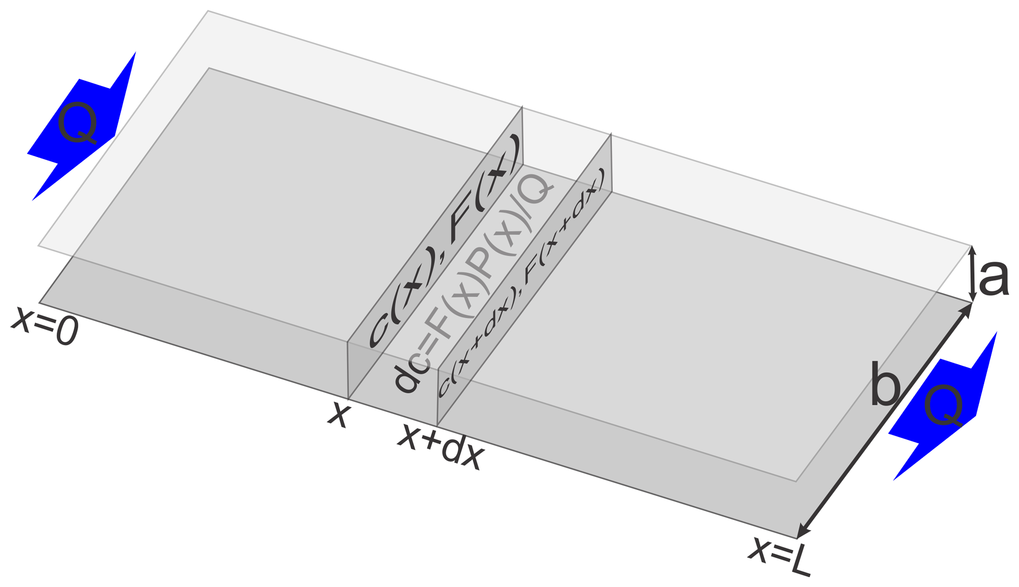
Figure 2Discretization and mass conservation in a basic network element; a 1-D fracture. The conservation of mass requires that the change in concentration dc in the section between x and x+dx is proportional to its surface P(x)dx, where P(x) is the perimeter. The change in concentration dc is also proportional to the dissolution rates F(x) and inversely proportional to the flow rate Q.
Mass conservation requires that the amount of calcite dissolved from the walls during the time interval Δt within any part of the fracture between x and x+Δx is equal to the difference between the amount of calcium leaving at x+Δx and the amount of calcium entering at x during the same time interval (see Fig. 2).
From this one obtains
Integration yields
For linear dissolution kinetics the dissolution rates are given by Dreybrodt et al. (2005a) and Dreybrodt (1988):
with
where k is the rate constant, ceq is the equilibrium concentration, and k1 is the rate constant of the surface reaction. This takes into account the common action of surface reactions and transport by molecular diffusion. For small aperture width, a, k is determined by surface reactions, whereas, for large a, k is governed by diffusion (Dreybrodt, 1988). This is close to the expression of k used by Szymczak and Ladd (2009).
For a uniform plane-parallel fracture, integration of Eq. (6) using Eq. (7) yields
where
λ is the penetration length, a distance along the fracture where the concentration and the dissolution rate has dropped to of its initial value at the input.
To obtain the temporal evolution of the profile of any fracture i, j in the net we discretize time and spatial variables t and x into suitable increments Δt and Δx and perform the following procedure (Dreybrodt, 1996):
-
Calculate Qi(t) by using Eqs. (1) to (3) for each fracture.
-
Calculate Fi(x) from Eqs. (8) and (7).
-
Calculate the new profile assuming a constant rate in the time interval Δt by
Discretization of the spatial variable x has to be done with care. The change in concentration Δc within the interval Δt is given by
The increments Δc are chosen such that changes in (ceq−ci) are small to avoid numerical saturation (Dreybrodt, 1996). From these, suitable Δx values are obtained. Otherwise wrong conclusions can be the result as in the work of Groves and Howard (1994), who claimed that for achieving breakthrough of a fracture a minimum aperture width is necessary.
3.1 Homogeneous net: the basic case
To get a first insight, we start with a homogeneous net with equal aperture widths a0=0.02 cm, equal widths b=100 cm, and equal lengths l=200 cm for all fractures. The net, shown in Fig. 1, consists of 151 nodes in both directions, which results in a dimension of 300 m by 300 m. At the left-hand input border, a hydraulic head h=15 m injects flow into all its fractures. The right-hand side output border is at h=0 and all fractures can drain water. The upper and lower boundaries have periodic conditions. Topologically this means that a 2-D domain is mapped onto a cylinder. This makes the evolution of fractures independent from their distance from the upper and lower boundaries, which is not the case if these are no-flow boundaries. This simulates a 1-D problem, where Szymczak and Ladd (2011) found the instability with respect to infinitely small perturbations, which causes the evolution of wormholes.
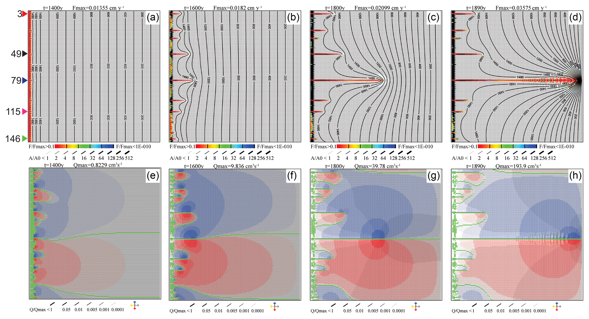
Figure 3Temporal evolution of a uniform fracture network. Panels in the upper row show aperture widths as line thickness and relative dissolution rates (a ratio between the rate in a fracture and the highest dissolution rate Fmax in the network) given in the color code. Lower panels show relative flow rates (ratio between the flow rate in a fracture and flow rate Qmax in the fracture with maximal flow in the network) and flow directions as shown by the arrow code. Green lines denote the flow divides by connecting nodes with opposite direction of outflow. White regions depict zero flow. Colored triangles mark the position of inputs where later wormholes evolve (See also Fig. 4). Numbers denote their y coordinate.
Figure 3 shows the temporal evolution of the aquifer. The upper panels illustrate the dissolution rates by a color code shown below and the fracture aperture widths by a bar code. The distribution of the hydraulic head is depicted by isolines in the upper panels. The lower panels depict the flow rates by the thickness of lines shown below and their directions by colors. Grey means flow downstream (left–right), blue is the direction along a transverse fracture from the lower boundary to the upper one (flow up), and red is flow in the opposite direction (flow down). Note that the flow rates are normalized to Qmax, which is the flow rate in the fracture with maximal flow in the entire network. They are depicted by a bar code. White regions exhibit flow rates less than 10−4Qmax.
After 1400 years, an almost even front of widening channels has propagated a few meters downstream (Fig. 3a). Flow (Fig. 3e), however, exhibits an uneven distribution. There are domains of transverse flow up (blue) and down (red) originating from the different wormholes.
After 1600 years, due to the instability caused by numerical noise, the front breaks (Fig. 3b and f) and many fractures protrude out from the previously even front. The domains of lateral flow have increased. The green color (Fig. 3e–f) connects nodes at the crests and troughs of the hydraulic potential field and, therefore, marks water divides between the lateral flows originating from the various channels.
After 1800 years (Fig. 3c and g), seven prominent channels have propagated into the net. Transverse flow from the leading channel dominates, whereas lateral flow from the channels staying behind becomes low, as shown by the white regions (Fig. 3g). After 1890 years, only one channel has reached the output boundary, whereas all others have almost stopped growing. Due to the redistribution of the heads, the leading wormhole ejects flow perpendicular to the isolines into the net, as can be seen from the red and yellow regions of dissolution rates close to its tip in Fig. 3h. The shorter losing wormholes are now located in a region with low hydraulic gradients. Therefore, flow in them is reduced.
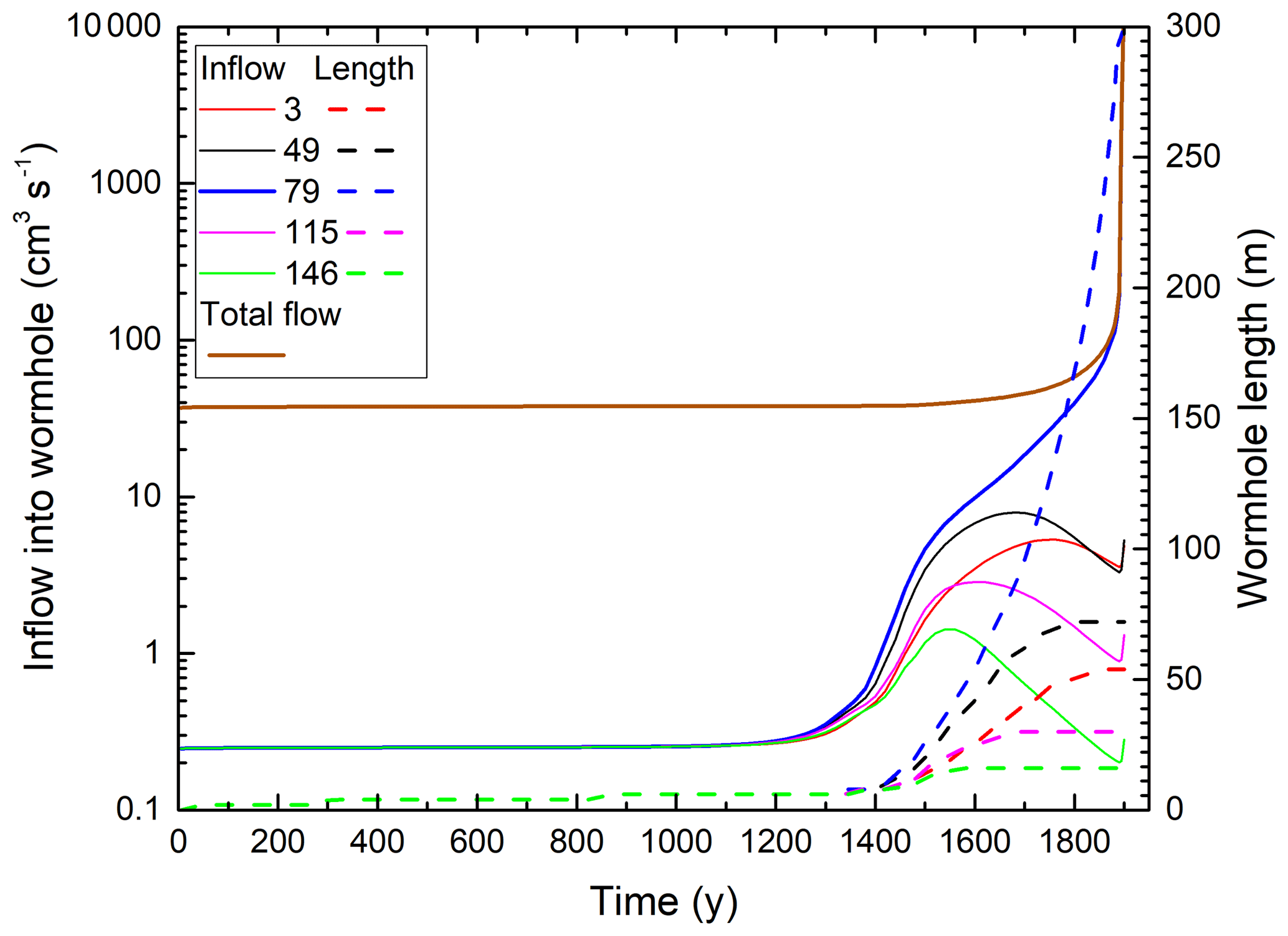
Figure 4Temporal evolution of the total flow through the network (solid brown line), input flow rates, and lengths of wormholes at different positions (given as a y coordinate of nodes).
Figure 4 depicts the temporal evolution of the total flow through the domain (solid brown line), flow rates into the inputs of the evolving wormholes (full lines), and their lengths (dashed lines) defined as the distance where . For the first 1000 years, during the evolution of the even dissolution front, the resistance of the net changes only inside the dissolution front close to the input. All input points transmit equal flow into the net. The total flow rate (37.5 cm3 s−1) equals the flow through one fracture (0.25 cm3 s−1) multiplied by the total number of input points (150). The flow into the input nodes of all later wormholes stays almost constant until after 1200 years, when one observes a rapid increase due to the wormhole formation.
Soon after, the curves separate, where more successful wormholes (at y=79, 49 and 3) gain flow on behalf of the less successful ones (at y=146 and 115). The flow into the latter reaches a maximum but then drops, and these wormholes stop growing. Between 1500 and 1600 years the winning wormhole (y=79) takes over the domain and increases in length until it reaches the downstream boundary of the domain. The regression of the remaining competitors continues until they stop growing.
3.2 Homogeneous network with one seed to trigger a single wormhole
In view of the results in Fig. 3, one asks for the detailed mechanisms by which the different wormholes compete for growth and the flow they carry. To this end it would be advantageous to deal with scenarios with only a few competing wormholes.
To this end we use the idea of Upadhyay et al. (2015), who have put seeds into the entrance region of the modeling domain consisting of areas with increased fracture aperture width with respect to the apertures widths in the net. This way the seed triggers wormhole growth from its region. To trigger the instability of the dissolution front, we insert seeds in the following way. Using the net of Fig. 3, we select some input point at the left-hand boundary. From there, we assign a fracture aperture width a+Δa to the first 10 horizontal (horizontal meaning parallel to the x axis) fractures in the downstream (left–right) direction. These fractures are marked in green in Fig. 5a. In order to keep the change in the net small, we chose Δa≪a0.
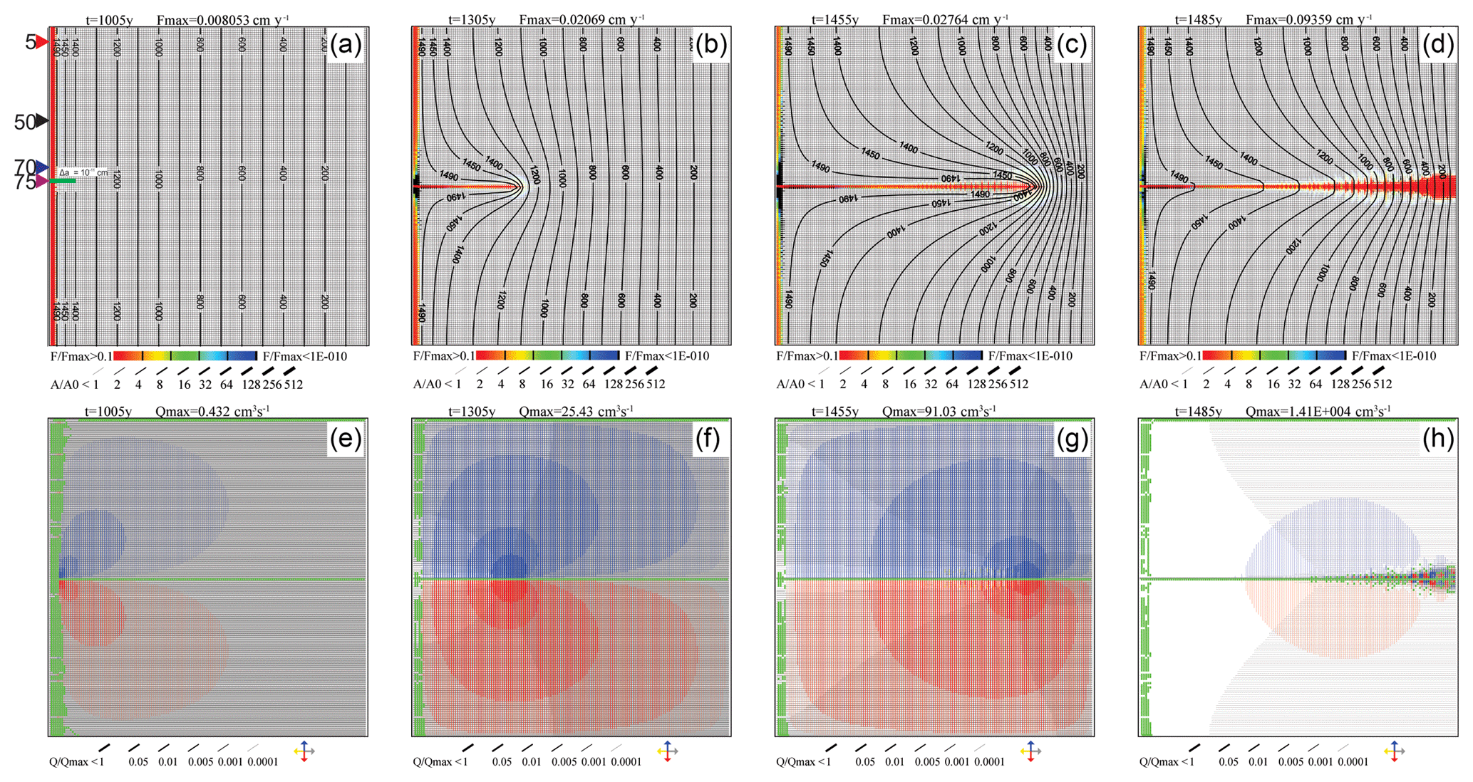
Figure 5Evolution of a seeded network. Same as Fig. 3 but slightly larger initial apertures by Δa=10–11cm are assigned to the first 10 fractures at position 75, denoted by green in (a).
Figure 5 depicts the evolution of a single wormhole initiated by a seed with cm at 75 nodes (150 m) from the upper boundary, the position along which the winning channel develops in Fig. 3. After 1005 years (Fig. 5a), the first few horizontal fractures are widened evenly such that a sharp reaction front is visible. Most of the flow is directed left–right, but at the position of the seed a region of transverse flow is visible (Fig. 5e). From there, a wormhole invades downstream, as shown in Fig. 5b at 1305 years. Its aperture width decreases with distance from its input. Dissolution rates inside the wormhole are high, as depicted by the red color, but they decline rapidly beyond its tip. The direction of flow and its magnitude are depicted by the lower panels (Fig. 5e–h). Most of the flow leaves the wormhole by flow up and down along the transverse fractures, as indicated by the thick blue and red lines close to its tip. As noted before, the line thickness gives a normalized flow rate Qf∕Qmax, where Qf is the flow through the fracture and Qmax is the maximal flow rate occurring in some fracture in the net. This way the total flow through the colored fractures amounts to about 95 % of the total flow through the domain.
With deeper penetration of the wormhole, the regions of transverse flow increase and high dissolution rates are active along the entire wormhole (1455 years; Fig. 5c and g). At 1485 years, shortly before breakthrough, the vertical fractures (vertical meaning parallel to the y axis) in the downstream region of the wormhole have experienced widening (Fig. 5d and h). Several small competing vertical wormholes have developed in a pattern similar to the reactive front of the smooth fracture in Fig. 3. This seems to be caused by the instability inherent to the model.
The high transverse flow rates are caused by steep transverse hydraulic gradients close to the wormhole. This can be envisaged from the lines of equal heads (isolines) shown in the top panels of Fig. 5. With increasing distance upstream from the tip of the wormhole, the flow rates decline because of decreasing hydraulic gradients. At the tip head, gradients in the horizontal direction rise, and consequently the flow rates increase in this direction (grey lines). Flow rates drop along the transverse fractures with greater distance from the wormhole because, at the junctions with horizontal fractures, flow is partly diverted into these horizontal fractures and then guided to the output at h=0 m.
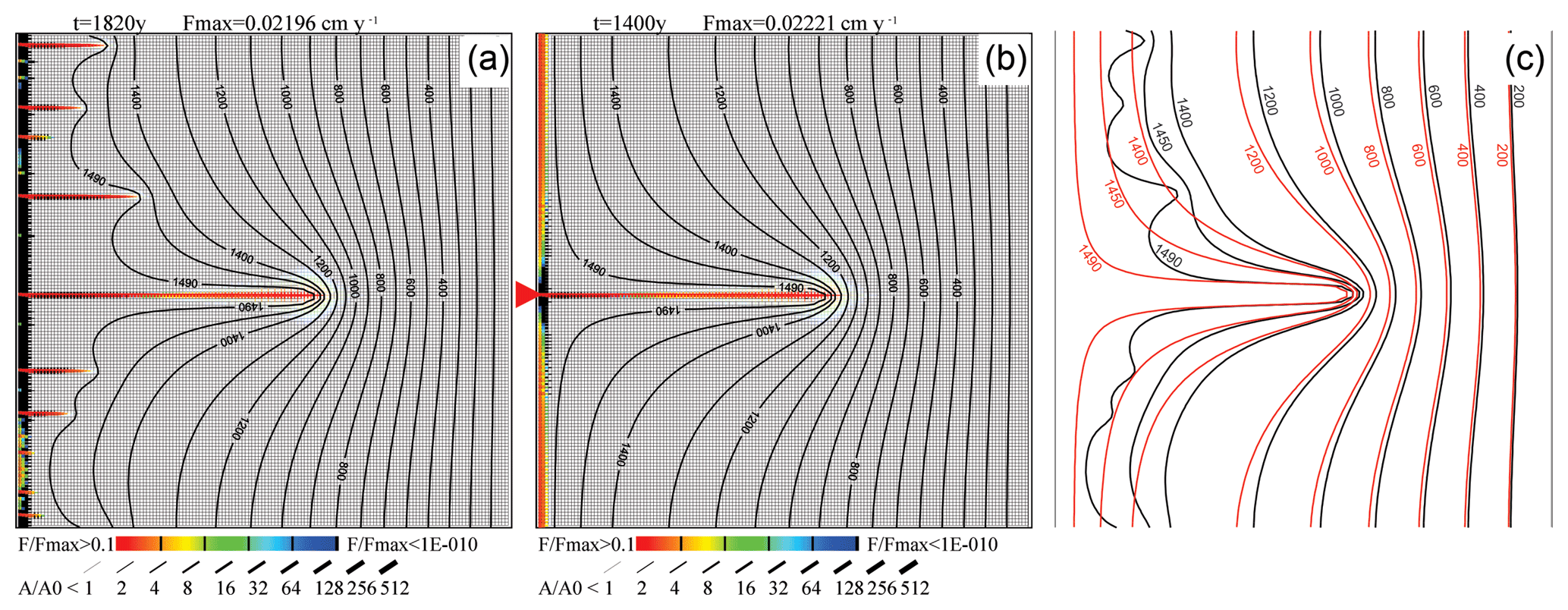
Figure 6Comparison between the case with no seeds (a, see Fig. 3) and single-seeded case (b, see Fig. 5) at equal length of the dominant wormholes. (c) Overlaid head distribution from a case with no seeds (a, black) and a seeded case (b, red).
3.3 Evolution of the winning wormhole
In Fig. 6, we compare the pressure fields of the evolution in Fig. 3 (no seeds, Fig. 6a) and Fig. 5 (one seed, Fig. 6b) at times where their channels have equal lengths. In Fig. 6c, their head distributions are compared. The black isolines show the head distribution for the scenario without seeds and the red ones with one seed. In the downstream region for heads smaller than 1200 cm, the head distributions become very similar. Therefore, the evolution of the leading wormhole seems to be independent of the presence of other wormholes. On the other hand, the fingers in the non-seeded (homogenous) case (Fig. 6a) would have grown deeper into the domain if the leading channel had not existed.
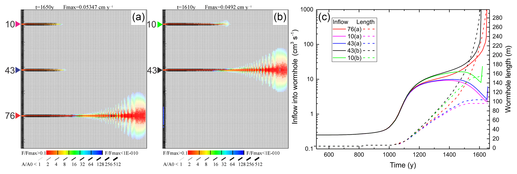
Figure 7Breakthrough situation in a network with (a) three seeds at positions 10, 43, and 76 and (b) two seeds at positions 10 and 43. (c) Evolution of input flow rates and wormhole lengths for seeded wormholes in (a) and (b). Note that the winning wormholes, black curve (43 b) and red curve (76 a), show a very similar behavior.
To explore this deeper, in Fig. 7 we compare the evolution of a scenario with three seeds at , and 76 (scenario a) and a scenario where the previously winning seed at y=76 is omitted (scenario b). The evolution in time is illustrated by the flow rates into the entrances of the wormholes (Fig. 7c).
In scenario a (Fig. 7a), until 1200 years, all flow rates are equal (Fig. 7c). Then, the instability causes an advantage for the flow rate through the input at y=76. The other two seeds, at 10 and 43, are inhibited, and flow through them stays constant and is reduced later, whereas flow through input at y=76 increases until breakthrough. If this winning seed is omitted (scenario b; Fig. 7b), the evolution of the flow rates into the inputs of the seeds at y=10 and 43 is identical to that in scenario a until 1100 years. Then, the seed at y=43 gains an advantage and inhibits the seed at y=10. The initial evolution of the flow rates in both scenarios up to 1100 years is identical for all seeded inputs. After 1200 years, in scenario a the leading wormhole gains an advantage, whereas the competing ones stop growing. In scenario b, this event happens 80 years earlier. The evolution of the winning wormholes observed from the time of this moment is identical. This confirms the idea that their evolution is independent of the presence of losing wormholes.
3.4 Evolution of a single wormhole
To understand the dynamics of the evolution of wormholes, we first investigate in detail the evolution of a single wormhole. Then, we study the competition between two wormholes, which are initiated by identical seeds at various distances from each other. Finally, a scenario with many seeds is shown.
We go back to Fig. 5, the scenario with a single seed resulting in the creation of a single wormhole. The high transverse flow rates are caused by steep transverse hydraulic gradients close to the wormhole. This can be envisaged from the head isolines shown in the top panels (Fig. 5a–d). With increasing distance upstream from the tip, the flow rates decline because of decreasing gradients. At the tip head, gradients in the horizontal direction rise, and consequently, although small, the flow rates in this direction increase (grey lines). Flow rates drop along the transverse fractures with lateral distance from the wormhole because, at the junctions with horizontal fractures, flow is partly diverted into them and then guided to the output at h=0 m.
Figure 8a illustrates the flow rates in the central fracture along the wormhole as a function of the distance from the input for various times. In the beginning, when the length of the wormhole is small, flow rates along the wormhole are low, and, due to outflow into the vertical fractures, the flow rate declines to a small value at its tip, which is determined by the overall flow resistance of the initial net. With increasing time and length of the wormhole, the vertical outflow increases, allowing rising input flow at the constant head boundary. Close to the tip, due to the flow out into the transverse fractures, flow along the wormhole declines to a value determined by the remaining resistance of the net. This behavior continues until breakthrough of the wormhole.

Figure 8(a) Profiles of flow rates along a wormhole at the given times. (b) Profiles of flow rates from the wormhole into the upper (black) and lower (red) domain at given times.
Figure 8b depicts the transverse flow up and down from the wormhole. In the beginning, when the wormhole is short, the transverse flow rates increase steeply by orders of magnitude until they reach a maximum close to its tip and then they decline rapidly. Note that the sum of the total transverse outflow along the wormhole and the longitudinal outflow at its tip must be equal to the inflow at its input. The region where the horizontal flow rates decline in Fig. 8a marks the region of major transverse outflow. When the length of the wormhole increases, this region is shifted deeper into the net and the maximum rate of flow becomes higher, marking the increase in total transverse outflow in time. Thus, the inflow of fresh solution, aggressive with respect to limestone, increases with increasing length of the wormhole supporting further dissolution along its entire length and at its tip. The vertical fractures carrying the transverse flow from the wormhole into the upper and lower domain are also subjected to the competition and wormholing, making some of these fractures more successful than others. This results in the nonuniform transverse pattern seen in Fig. 7a (wormhole at y=76) and Fig. 7b (wormhole at y=43) and apparent “noise” in lines 4 and 5 on Fig. 8b.
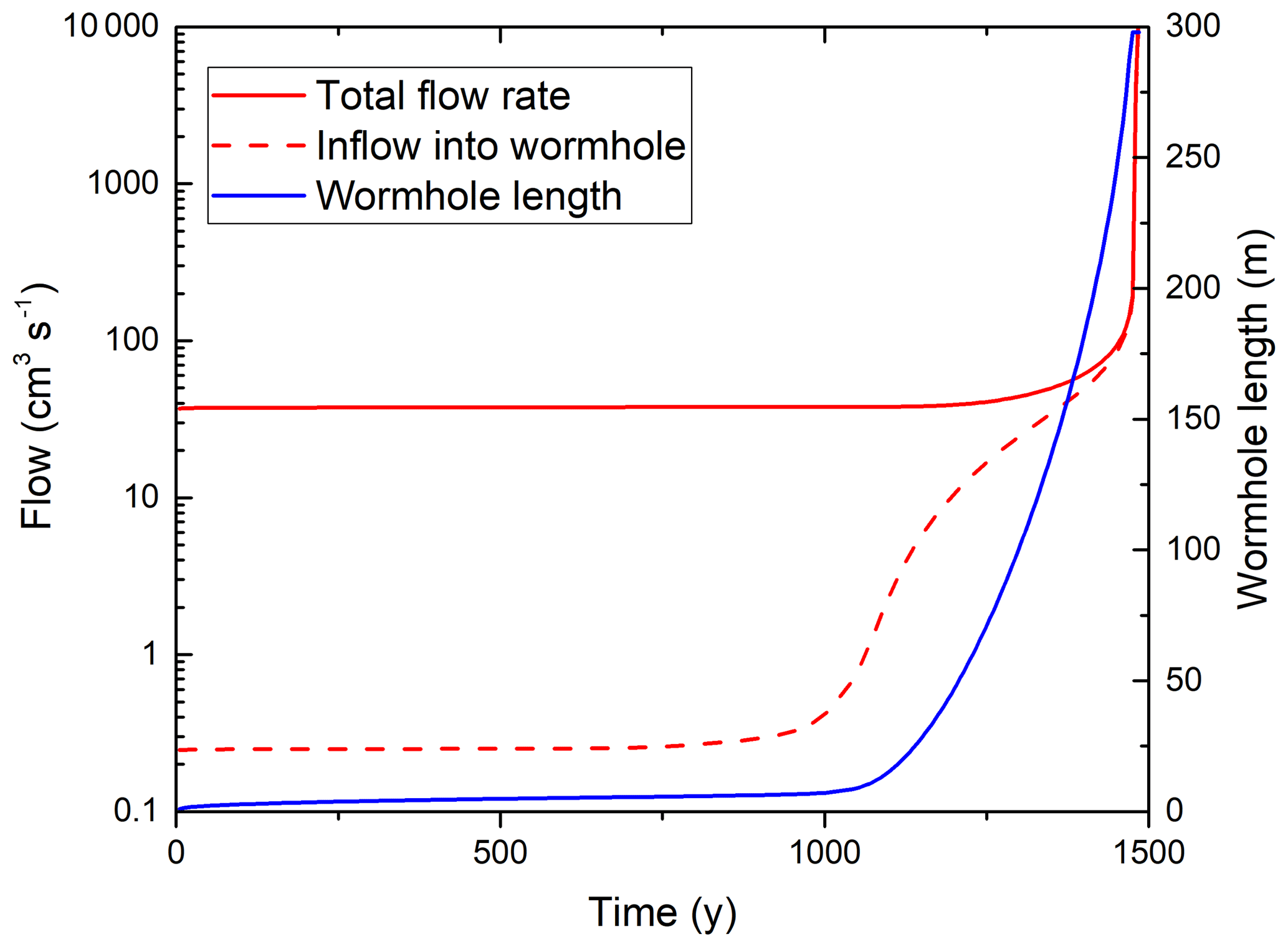
Figure 9Evolution of total flow through the network (full red line), input flow into the seeded wormhole (dashed), and length of the wormhole (blue line).
Figure 9 shows the temporal evolution of the total flow through the domain, the flow rate into the input of the wormhole, and the length of the wormhole. In the beginning, flow into the wormhole is low and given by the resistance of the net. For the first 1000 years, flow remains almost constant. During this time, the solution front progresses evenly. Then, the instability causes initiation of the wormhole and flow through it rises. With increasing length of the wormhole, the resistance between the tip and the output becomes smaller, and Qtot grows until at breakthrough it rises rapidly.

Figure 10Profiles of aperture widths (solid lines) and saturation ratios (c∕ceq, dashed lines), along the wormhole at given times.
To get more insight, in Fig. 10 we have plotted the aperture widths (solid lines) and the saturation ratio c∕ceq (dotted lines) along the line of the downstream fractures guiding the wormhole for various times of its formation. c∕ceq increases steadily until it reaches saturation at the tip of the wormhole. There, dissolution rates drop to almost zero. The aperture widths along the first two-thirds of the wormhole length are on the order of centimeters.
The following questions arise. How important is dissolution in the net adjacent to the wormhole? Is its increase in permeability sufficient to create a feedback or is it of only minor influence? To answer these questions, we have investigated a scenario where only the walls along the line of horizontal fractures along the wormhole are soluble and the walls of all remaining fractures in the net are insoluble. Figure 11a depicts a comparison between the input flow rates in scenarios with and without dissolution in the net.
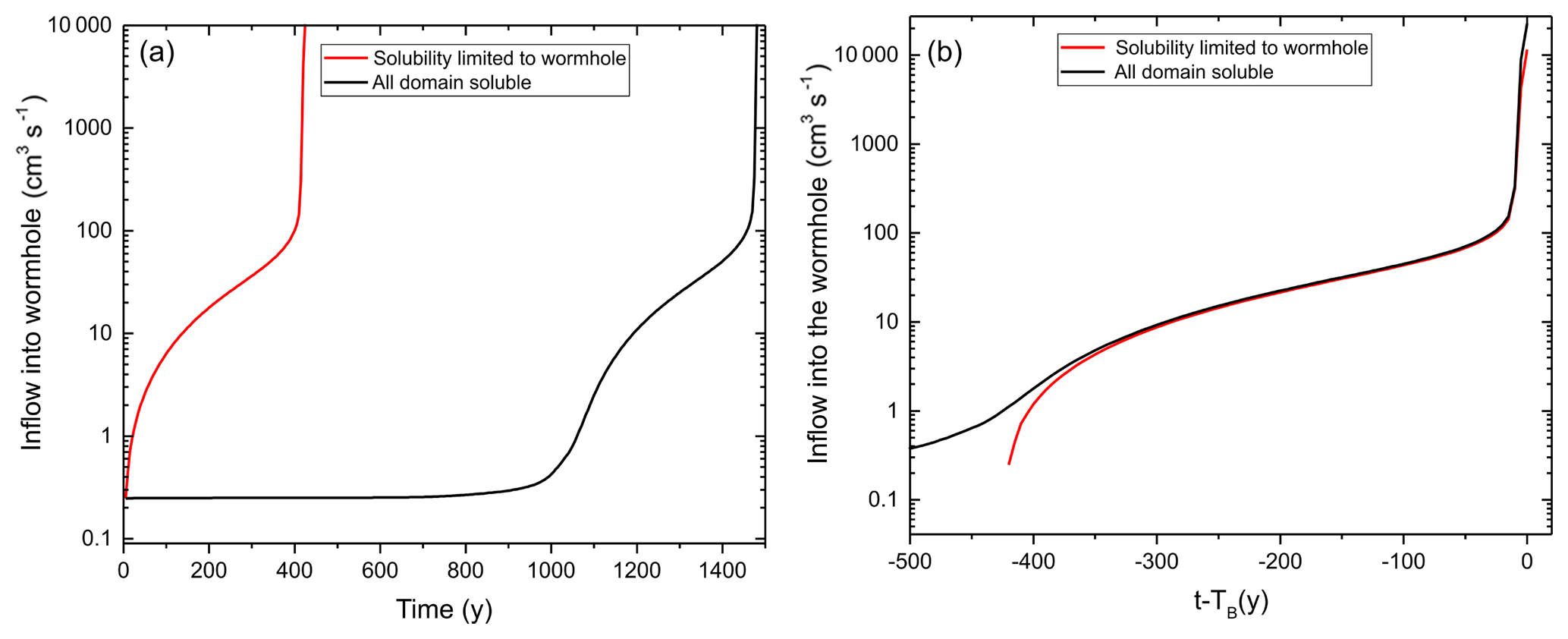
Figure 11(a) Evolution of inflow into the wormhole for the case where solubility of fracture walls is limited to the position of wormhole (red line) and the case where the complete network is soluble (black line). (b) Same cases as in (a), but the horizontal axis is defined as the time minus the breakthrough time for each case (t−TB).
For a net of soluble fractures, there is a long time of low constant flow due to the even solution front propagating slowly downstream. As long as the dissolution front is completely uniform, transverse flow is not possible and enhancement of dissolution triggered by transverse outflow is absent. Each fracture behaves as an isolated fracture. As soon as the instability gives advantage to one fracture it can eject transverse flow and start to grow rapidly until breakthrough is attained.
When the fractures of the net are insoluble, except those of the wormhole, an even dissolution front cannot be established. The line of soluble fractures along which the wormhole propagates gains an advantage immediately and reaches breakthrough in a much shorter time. It is important to note that the temporal evolutions of the breakthrough curves are almost identical if one compares them from the time where flow exceeds 1 cm3 s−1. Figure 11b shows an overlay of the two curves by shifting the time by −TB to t−TB. This gives evidence that the resistance of the net in both cases is almost equal or, in other words, that dissolution outside the leading fracture is practically absent during the evolution of the aquifer.
We therefore postulate that the main mechanism causing progression of the wormhole is an increase in the input flow caused by ejection of transverse flow into the net. In conclusion, the following feedback mechanism seems to be plausible. As soon as one wormhole, for whatever reasons, becomes longer than the neighboring ones, it emits transverse flow that increases its input flow. The resulting enhanced dissolution capacity increases the length from where transverse flow can be emitted, and, consequently, the amount of outflow increases (see Fig. 8) causing growing inflow. It is interesting to note that for a net of soluble fractures the advancing dissolution front retards breakthrough considerably.
3.5 Interaction between two wormholes
In the next step, we study the interaction of two wormholes growing simultaneously. We construct a net with two seeds, at the various positions as shown in Fig. 12, which illustrates the temporal evolution of the aquifer. We start with the two middle panels (Fig. 12b) depicting the evolution of a domain with two seeds located at y=60 and y=90. Until about 1000 years, all the fractures of the net widen evenly such that a sharp front of wider fractures propagates into the domain (not shown). After 1200 years, two wormholes have intruded from this front at almost equal length. In this symmetric scenario, the analytic solution would exhibit equal length of the wormholes until breakthrough. Due to the instability, however, this symmetry is broken and the wormholes develop at different rates. The upward and downward transverse flow patterns from the upper wormhole become strikingly different, in contrast to an isolated single wormhole where both corresponding patterns are symmetric. Due to the presence of the second wormhole, the transverse hydraulic gradients in the region between the wormholes are reduced significantly in comparison to those in the outside regions. Because of the slightly different lengths of the two wormholes, the inflow of aggressive water into the upper wormhole is lower than that into the one below. Therefore, the lower wormhole grows faster, causing increased inflow.
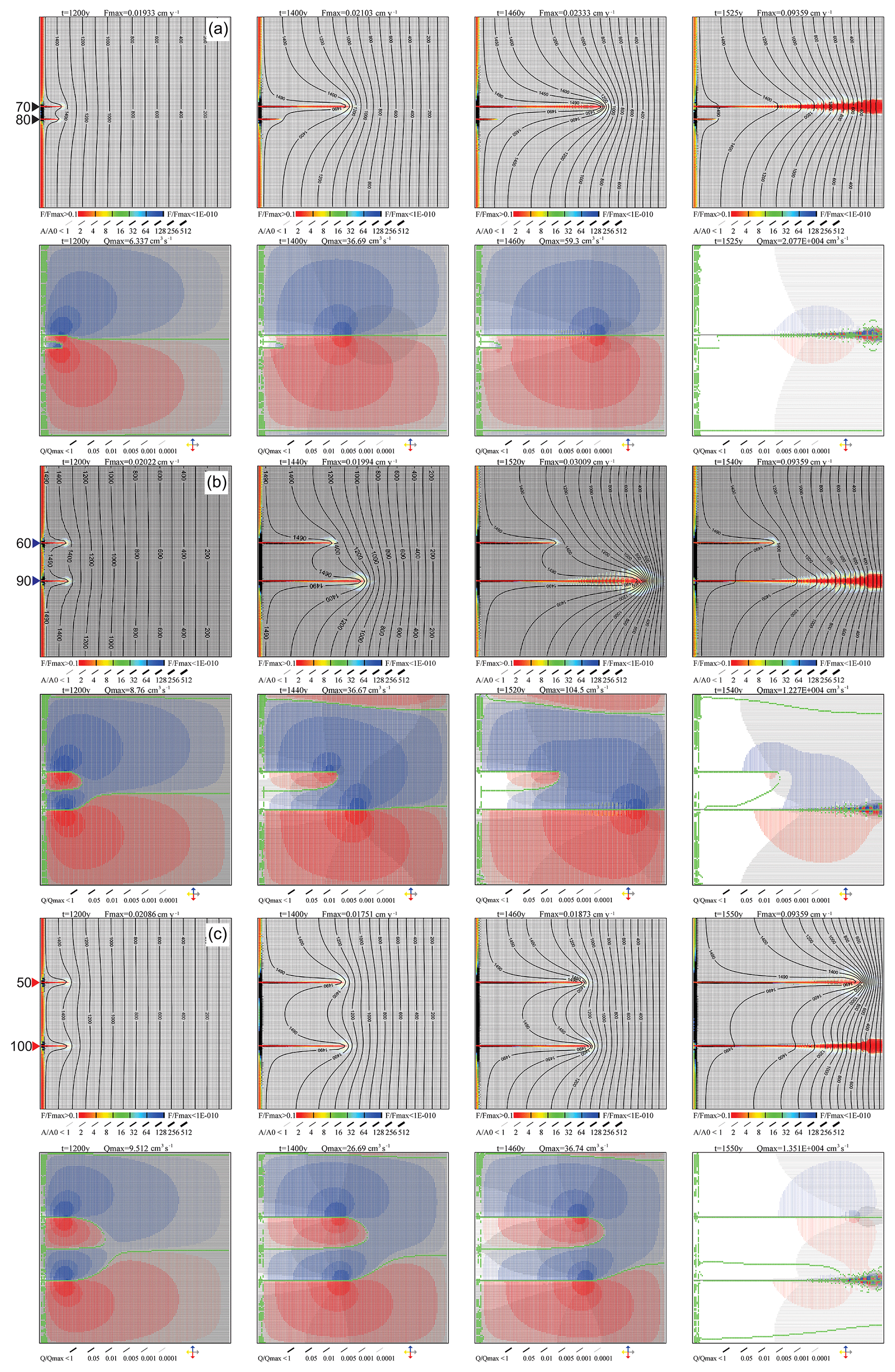
Figure 12Interaction of two wormholes seeded at distances of 10 (a), 30 (b), and 50 (c) nodes. First rows of panels for each case show aperture widths and relative dissolution rates; second rows show flow rates and directions. All codes and conditions as described in Fig. 3.
Figure 13 shows the dissolution rates and flow rates along the two wormholes at y=90 and y=60 for various times during their evolution. As long as the length of the wormholes are close to each other (until 1200 years) their patterns are almost equal, and therefore the flow into the two wormholes is almost equal as well. With increasing length, the inflow into the faster growing wormhole increases, whereas that of the delayed one rises only slightly until it declines. This is reasonable because its outflow is inhibited by the faster growing wormhole. If, however, the distance down flow between their tips exceeds some limit, the flow through the shorter wormhole decreases.
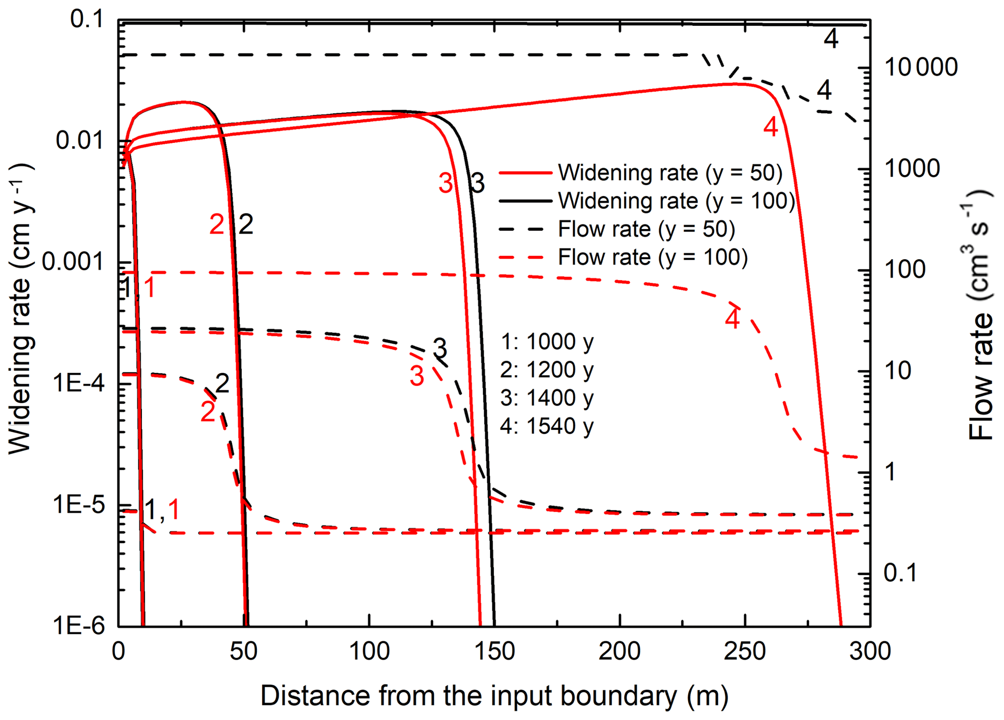
Figure 13Profiles of widening (full lines) and flow rates (dashed lines) for the case with seeds at y=60 (red) and y=90 (black) nodes from the top (Fig. 12b).
Figure 14 depicts the temporal evolution of the lengths and the input flow rates of the two wormholes for all three scenarios in Fig. 12 until breakthrough. The middle panel (Fig. 14b) depicts the scenario discussed here. In the initial state, the lengths are equal as expected. When the instability becomes active, the lower wormhole grows rapidly, whereas the upper one experiences delayed growth. The same behavior is exhibited by the input flow rates. This pattern is characteristic for the onset of instability in nonlinear systems.
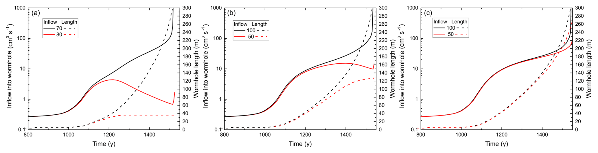
Figure 14Temporal evolution of flow (full lines) and length (dashed lines) of the interacting wormholes of Fig. 12. Labels corresponds to Fig. 12.
From these findings, one may conclude that the interaction between the wormholes depends on the distance between them in the y direction. If this distance becomes sufficiently large that the transverse flow from both wormholes into the region between them has decayed to zero at a distance of less than half of the separation between the wormholes, we have a situation equivalent to that of an isolated wormhole. This defines a “region of influence” as suggested by Rajaram et al. (2009). If two growing wormholes are located within this region of influence, only one of them will achieve breakthrough.
To give further evidence we study a scenario with two seeds as above but with increased distance between them, which is larger than the distance of influence. The lowest panels in Fig. 12 show the evolution of a domain with two seeds at y=50 and y=100. Both wormholes invade into the net at almost equal speed until breakthrough (Fig. 12c). To illustrate the region of influence, the lower panels show flow directions by color. In addition, all fractures with flow less than 10 are shown in green. These green borders define the areas that cannot be crossed by transverse flow. They separate the domains of flow upward and downward from the wormholes. There are three borders extending from the tips downstream and one in the middle between the domains. They end in a region downstream where flow essentially becomes horizontal (i.e. parallel to the horizontal axis). With increasing length of the wormholes, this region of horizontal flow is shifted closer to the output. A further region of zero transverse flow extends from the input boundary between the wormholes. For all stages of evolution, the flow domains of both wormholes remain clearly separated, and both wormholes grow independently of each other.
If, in comparison to Fig. 12b, the distance between the seeds becomes smaller as illustrated in Fig. 12a, one expects increasing dominance of the winning wormhole. At 1400 years, the two competing wormholes exhibit similar lengths in Fig. 12a and b. At later times, however, the losing wormhole stops growth in Fig. 12a, whereas it still gains length in Fig. 12b.
The evolution of flow and length for the three distances is shown in Fig. 14. With increasing distance the time needed to gain advantage for the winner increases until both wormholes become too distant to interact and propagate at the same pace.
3.6 Interaction in an array of wormholes
From these findings, we conclude that if several wormholes are located inside the region of influence of one another, only one of them will reach breakthrough. This is illustrated in Fig. 15, where 10 seeds are inserted at distances of 30 m. After 1200 years, all seeded wormholes have developed to almost equal lengths. Due to the instability, the wormholes start to grow with differing speeds. At this point, it is not possible to predict the further evolution.
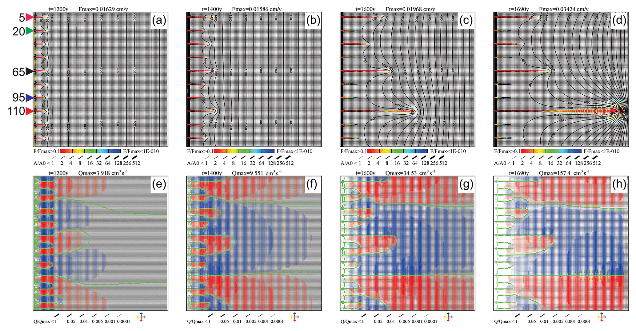
Figure 15Interaction of set of wormholes seeded at the distance of 15 nodes. Triangles and numbers denote location and y coordinates of inputs into the selected wormholes.
After 1400 years, three wormholes (at , and 110) have won a lead and have inhibited the growth of all their neighbors. The wormhole at y=110 has advanced further than its competitors. Therefore, these are also delayed and ultimately lose. Figure 16 shows the temporal evolution of inflow into marked wormholes and their lengths.
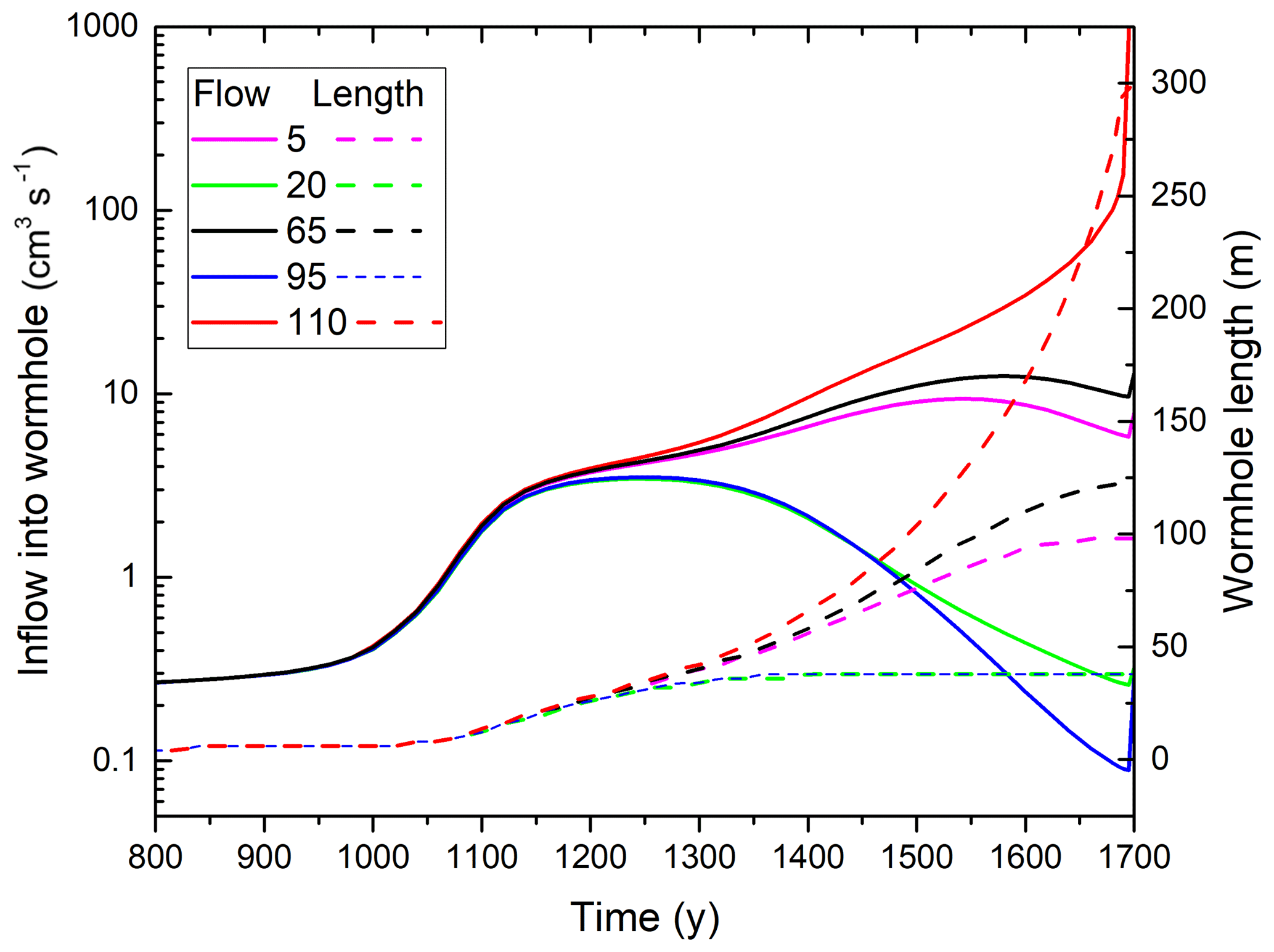
Figure 16Evolution of input flow rates (solid lines) and wormhole lengths (dashed lines) for the wormholes marked in Fig. 15.
At the beginning, flow through all fractures is equal. After 1100 years, the instability causes an advantage for wormholes at , and 110 and flow rates there increase (Figs. 15 and 16). Wormholes at y=20 and y=95 are in the region of influence of wormholes at y=5 and y=95 and, hence, stop growing. The same happens for wormholes at y=5 and y=65 100 years later.
From what we have found so far, the following picture of the evolution of a homogeneous net as described in Fig. 3 arises. Due to the instability of the system to small perturbations (Szymczak and Ladd, 2011), the initially uniform propagation of all equivalent fractures breaks down and some fractures gain advantage. The evolving pattern at that stage is not predictable. After some short time, however, the interaction of the different wormholes determines the head distribution and the flow rates in the entire net. The further evolution proceeds in a deterministic way. Nevertheless, the final patterns are predetermined by the initial instability.
For homogeneous nets with seeds, as in Fig. 14, where an analytical solution predicts equal lengths for all wormholes starting at individual seeds, the final patterns show wormholes only along the directions of the seeds. From this, one can suggest that for heterogeneous nets containing percolating pathways of fractures with aperture widths differing from those in the net, the wormholes should develop favorably along parts of these percolating pathways by a deterministic process where the instability plays no role.
Figure 17 gives an example of a dual network, where a net of prominent fractures with aperture widths of A0=0.03 mm is superimposed over the homogeneous net with aperture widths of 0.02 mm. The crude net of prominent fractures is discretized into elements of 20 m by 20 m with an occupation probability of 0.72. This way percolating pathways from the input boundary to the output boundary are assured. The prominent fractures are shown as thick lines in Fig. 17.
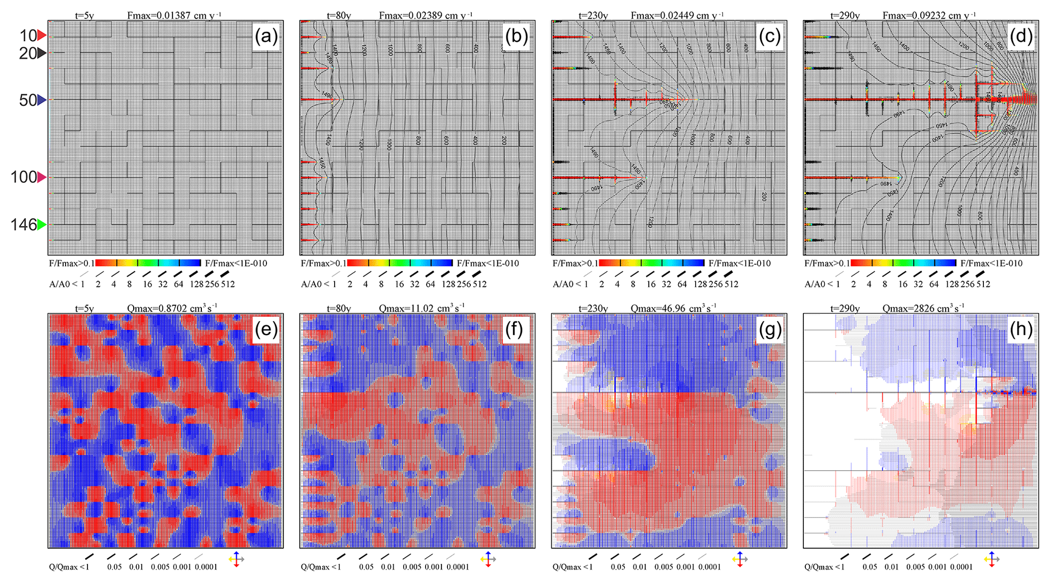
Figure 17Evolution of wormholes in a dual network. The network is a superposition of the basic network (Fig. 3) and a crude net of prominent fractures with A0=0.03 cm, length 20 m, and occupation probability 0.72. (a–d) Aperture widths and dissolution rates. (e–h) Flow rates and directions.
After 5 years in the dual network (Fig. 17a and e), small wormholes of equal lengths have developed along all the prominent fractures originating from the input boundary because the prominent fractures act as seeds. This prevents the creation of an even dissolution front along all the inputs without prominent fractures. After 80 years (Fig. 17b and f), wormholes of differing lengths have invaded the domain. The leading one inhibits further growth of all others, as can be seen after 230 years (Fig. 17c and g). After 290 years (Fig. 17d and h), the winning wormhole achieves breakthrough. It is interesting to note that introduction of prominent fractures reduces breakthrough time from 1900 years in the homogeneous net to 290 years (see Fig. 3). There are two reasons for this. First, an even dissolution front cannot evolve because perturbations from one-dimensionality are strong. Second, due to the wider prominent fractures along the pathway and also transverse to the winning channel, input flow is greater than along a pathway with fracture aperture width of 0.02 mm exclusively. Therefore, more calcite can be dissolved and the wormhole proceeds faster to breakthrough. For completeness, Fig. 18 illustrates the flow rates into the evolving wormholes and their lengths.
Another way to break the action of the instability is to select distinct input regions or input points instead of an even head along the entire input boundary. Such cases have been explored in Dreybrodt et al. (2005a).

Figure 18Evolution of input flow rates (solid lines) and wormhole lengths (dashed lines) for the wormholes marked in Fig. 17. Numbers on curves denote the y coordinates of the wormholes.
From our findings so far, we can summarize the evolution of wormholes as follows.
In Fig. 19a, we show the temporal evolution of the inflow into the winning wormhole for the basic case (see Figs. 3 and 4) in comparison to the evolution of the same domain with one seed implanted (see Fig. 5). In both cases we find a long initial period of about 1000 years during the formation of the even dissolution front with low, almost constant inflow. In both cases the instability becomes active, but in the seeded domain this happens about 400 years earlier. After the activation of the instability, a fringe with several small channels evolves and flow rates rise slightly to a few tenths of a cubic centimeter per second. In the unseeded case, several wormholes grow from this fringe with almost uniform rate until one of them has gained an advantage in its length and from then on develops independently of its past history. If only one line of fractures connecting the input to the output boundary is soluble and all other fractures in the net are insoluble, competition is excluded and the evolution of a dissolution front is thus not possible, so that the wormhole starts to grow immediately. In all cases shown in Fig. 19, the evolution of the wormhole is almost identical from the moment when it has gained an advantage over its competitors. This is shown in Fig. 19b where we have shifted each curve by its breakthrough time TB. In a nutshell, once a wormhole has gained an advantage over its competitors it grows independently of its former history and its evolution is determined by the structure of the domain. This means that the development of a uniform dissolution front retards breakthrough.
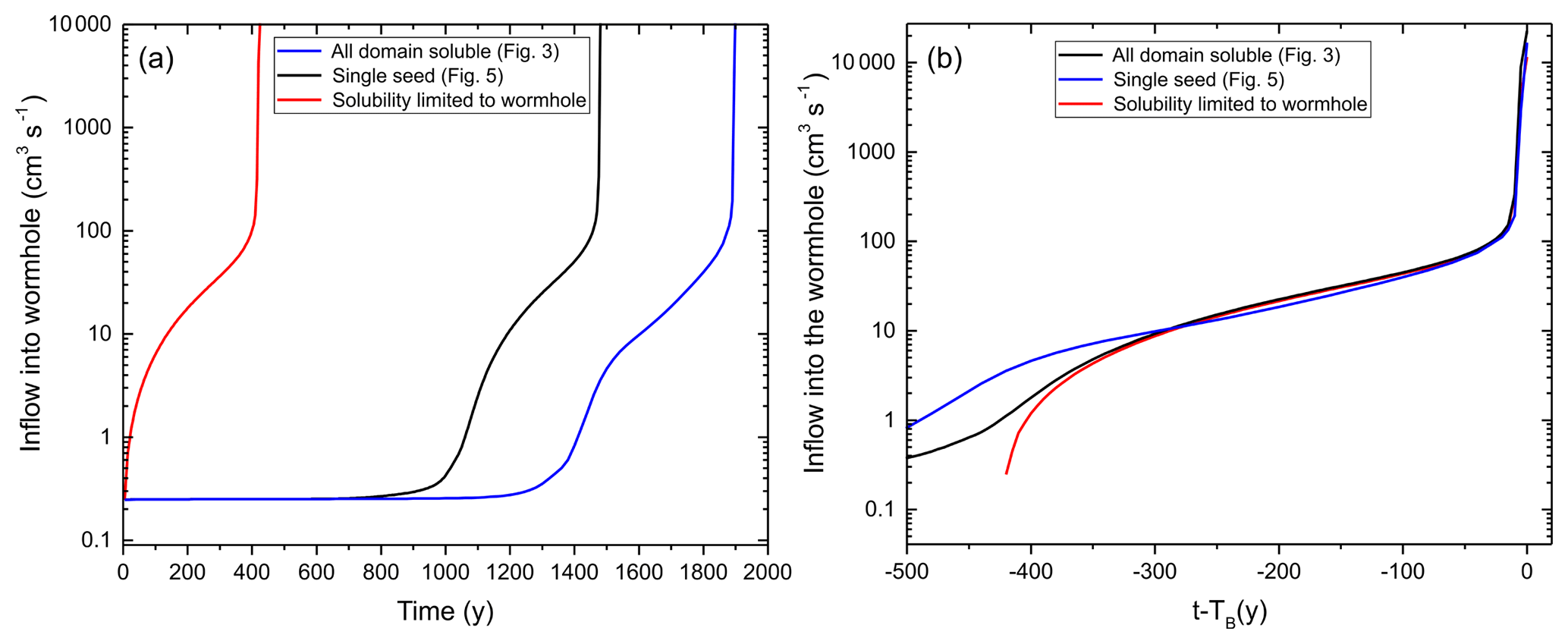
Figure 19Inflow into the wormhole as a function of time (a) and as a function of time distance to the breakthrough time (b) for the uniform network (blue line, Fig. 3), for the single-seeded case (black line, Fig. 5), and for the case where only the fractures along the wormhole are soluble (red line).
Figure 20, as a further example, illustrates the evolution of a heterogeneous domain with statistically distributed fracture aperture widths. These are taken from a lognormal distribution with amin=0.015 cm, apeak=0.02 cm, amax=0.025 cm, and σ=0.2 cm. There is no appearance of an even dissolution front but instead several competing wormholes start to grow immediately. After 300 years, one of them becomes dominant and breakthrough is achieved after only 560 years.
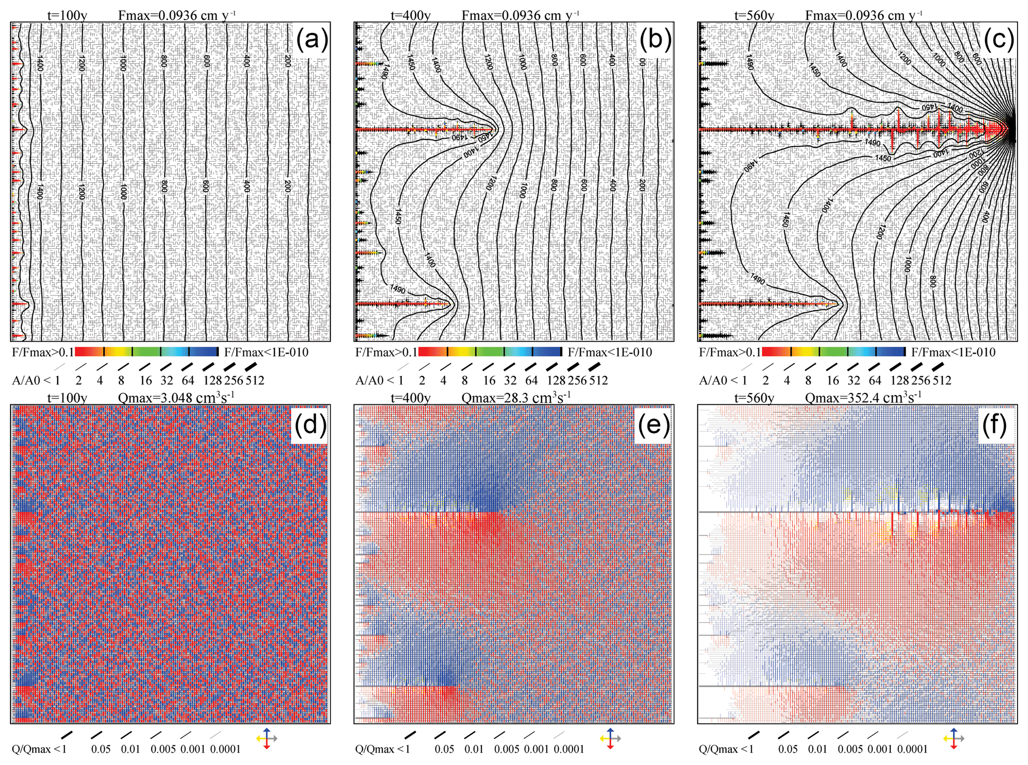
Figure 20Evolution of wormholes in the network with lognormal distribution of initial aperture widths. (a–c) Aperture widths and dissolution rates. (d–f) Flow rates and directions.
Compared to a single 1-D fracture of the same dimension (300 m × 300 m), the breakthrough times of the same fracture embedded into a two-dimensional array of fractures are lower by at least 1 order of magnitude and independent of the kinetic order of the dissolution kinetics (Dreybrodt et al., 2005b; Szymczak and Ladd, 2011).
To understand this, we go back to the evolution of the wormhole in a homogeneous aquifer with one seed. Figure 21a shows, for various times, the profiles of dissolution rates converted to widening of the fractures in centimeters per year and the concentration c∕ceq along the fracture. In Fig. 21b the profiles of the aperture widths, the flow into the wormhole, and the penetration lengths are depicted. The penetration length, λ, is the distance of exponential decay from the given location, defined in Eq. (8). It is given by , , where a and b are the aperture width and breadth, Q the flow in the fracture at this position, and ceq the equilibrium concentration with respect to calcite. The effective reaction rate k is . Here D is the constant of molecular diffusion and k1 is the rate constant of the surface reaction. ( mol cm−2 s−1, mol cm−3, cm2 s−1).

Figure 21Profiles of different parameters at given times for the single-seeded case (network evolution presented in Fig. 5). (a) Widening rates (black lines, cm yr−1) and saturation ratio (red lines, c/ceq); (b) flow rates (black), penetration lengths (red), and aperture widths (blue).
With increasing a,k decreases and the penetration lengths increase accordingly in time at all locations in the wormhole, where dissolution is active. In the upstream part, where flow is large, they are on the order of several tens to hundreds of meters. The saturation, c∕ceq, of the solution increases slowly to about 0.8 close to the tip of the evolving wormhole, and widening of the fractures is active along the entire length of the wormhole. At its tip, the aperture widths decline rapidly and k increases accordingly. Consequently, the penetration lengths decline to a value of a few centimeters, and dissolution practically stops in fractures beyond the wormhole.
At each location in the fracture, penetration length increases with time. Therefore, dissolution can penetrate deeper into the fracture and the length of the wormhole increases. With increasing length, the amount of outflow from the wormhole into the net increases, and the flow into the wormhole grows because the effective resistance of the part downstream from its tip is reduced. Therefore, penetration lengths increase and cause deeper penetration of the wormhole into the aquifer. Here, the feedback loop is related to the resistance of the net into which it is embedded.
We have, therefore, explored a scenario where all horizontal fractures (i.e. parallel to the x axis) at y=150 have aperture widths A0=0.02 cm, while the rest of the fractures have generally different initial aperture cm. Figure 22 shows the dependence of the breakthrough times on the aperture widths of the net with A0=0.02 cm for various a0. If the fractures of the network are closed (a0=0 cm), the fractures with A0 are isolated and cannot exchange any flow with the network. It is, therefore, equivalent to a single 1-D fracture. The breakthrough time is 4×10⁶ years. With increasing a0, the breakthrough time decreases to 800 years at a0=0.0175 cm and the resistance of the net is reduced, favoring flow from the central fracture into the net. If a0 comes close to A0, the central fracture behaves like a seed and an even dissolution front arises. This retards breakthrough. In natural environments, the perturbations are generally large such that even dissolution fronts are prevented. Since the breakthrough times depend heavily on the unknown complex properties of the surrounding aquifer, it is not possible to predict breakthrough times. This example shows that with increasing amount of water, which can flow from the fracture into the net, breakthrough times are reduced and the instability does not arise because the surrounding net breaks the condition of one-dimensionality. Only when the perturbation is small, even dissolution fronts develop. This scenario was already discussed in Dreybrodt et al. (2005a).
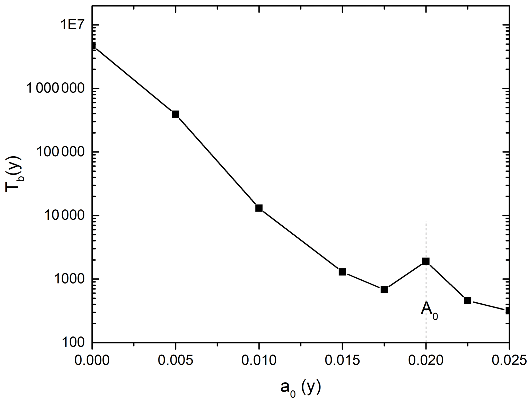
Figure 22Breakthrough time of a network with a central fracture A0=0.02 cm embedded into a network of fractures with initial aperture a0 as a function of a0.
In our model, the basic element of the 2-D net is treated as a 1-D fracture. This has been criticized by Szymczak and Ladd (2011). They argue that, due to the inherent instability, the fracture will not be widened evenly but wormholes will arise and the breakthrough time will be reduced. Wormholes, however, are created only in a limited range of Péclet and Damköhler numbers (Szymczak and Ladd, 2009). The Péclet number, Pe, is defined as and the Damköhler number, Da, as , where v is the velocity of flow and is given by . Another important parameter for the formation of wormholes is the penetration length of concentration, . Wormholes occur for Da>0.01 and Pe between 10 and 1000. For Da<0.01 and Pe>1, however, the dissolution front is compact and uniform and the fracture can be described by the 1-D approach. In our model, the initial velocity, v0, is 0.125 cm s−1 (see Figs. 8a and 9). With this value one obtains Pe=250 and Da=0.00032, and the initial penetration length is Lp=16 cm. With such conditions, widening of a fracture is likely in the range of a uniform dissolution front, but wormholes cannot be excluded because the values of Pe and Da are close to the border between wormhole formation and uniform dissolution (Szymczak and Ladd, 2009, Fig. 6). In the 2-D simulation of a single wormhole (see Fig. 5), we observe the penetration of an even dissolution front limited to the first five fractures until, after 1000 years, the instability breaks this front and the wormhole starts to develop. During this time, all fractures directed downstream exhibit identical dissolution and transverse flow is absent (see Fig. 9). Once the instability sets in, transverse flow rises sharply, and, consequently, also the flow rates along the wormhole increase (Fig. 9). Therefore, the flow velocity in the fractures upstream from the tip of the wormhole rises by at least 1 order of magnitude, and the penetration length takes values close to the length of the single fracture element. The Pe and Da−1 numbers rise, and the evolution of the corresponding 1-D fractures is shifted deeper into the region of uniform compact dissolution. In other words, all fracture elements of the net behave like 1-D fractures, which makes our model a reasonable approximation.
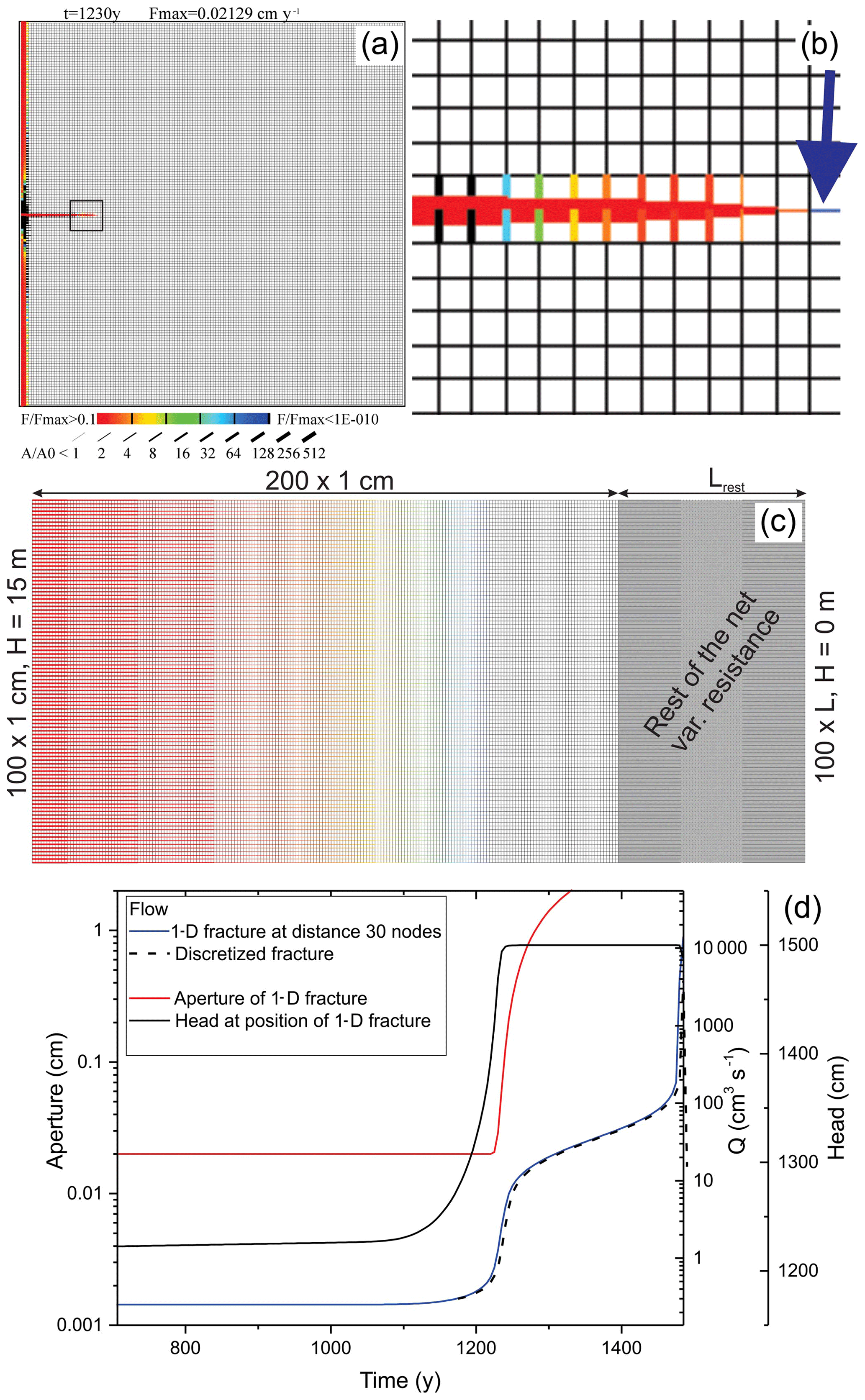
Figure 23(a) Two-dimensional network with penetrating wormhole. (b) Excerpt of an area marked by a square in (a) . Blue arrow marks the position of a fracture discretized into the 2-D domain. (c) Two-dimensional model of an elementary fracture. It shows a front of even dissolution. Right-hand part (grey rectangle) shows a set of parallel fractures with time-dependent resistances, appended to the outlet of the 2-D fracture. (d) Evolution of aperture width (red line), hydraulic head at the input (black line), and flow rate (blue line) for the fracture marked by an arrow in (b). Evolution of flow rate in a 2-D analog is shown by the dashed black line.
To verify this finding we have employed the following approach (Fig. 23). We consider a fracture that has just been reached by the wormhole (Fig. 23a, b). It has experienced almost no dissolution so far. We discretize this fracture into a network of 100 by 200 fractures, each 1 cm long and 1 cm wide with aperture width of 0.02 cm. (Fig. 23c). Figure 23a shows the 2-D net with the wormhole and the even dissolution front. A square marks the region enlarged in Fig. 23b, where the fracture of interest, at the tip of the wormhole, is marked by the blue arrow. Figure 23c depicts the discretization of this fracture and the dissolution front that is created in it after some time. The downstream boundary nodes of the fracture are connected to insoluble fractures with length L, an aperture width of 0.02 cm, and a width of 1 cm representing the remaining downstream resistance of the network. Figure 23c represents also the model domain for the simulation of the discretized 1-D fracture. To account for the increasing flow through this fracture, the length L is chosen such that the total flow through the fracture is equal to the flow in the corresponding fracture in the 2-D simulation. The simulation of the discretized fracture is performed until the breakthrough time of the 2-D model. Figure 23d depicts the evolution of hydraulic head (black line), aperture width (red line), and flow through the fracture (blue line). Until 1000 years, the head and, consequently, the flow remain constant. Then, caused by the intruding wormhole, head and flow rise. When the wormhole has reached the fracture (at t=1250 yr), the head reaches its maximal value equal to the head at the input. The further increase in flow is caused by the wormhole penetrating towards the exit in the 2-D simulation, reducing the resistance of the remaining net. This flow is shown by the dashed black line. In this way, we find wormholes only in the first three fractures in the 2-D net located in the pathway of the wormhole. For all the other fractures, downstream along the wormhole only even and compact dissolution fronts are observed.
In the first three 1-D fractures an even front develops initially. Due to the instability the front breaks down and wormholes grow there after 1200 years. In contrast, in all the following 1-D fractures downstream, due to the increasing flow after the 2-D-wormhole has arrived there, the Péclet number rises sharply by about 1 order of magnitude within a few tens of years. Therefore these 1-D fractures exhibit an even dissolution front. In our model we have assumed that in each junction of fractures lateral head differences are smoothed in such a way that at the downstream input fractures constant head conditions can be applied. Piotr Szymczak in the interactive comment regarding this work has argued correctly that this assumption is dubious “as the pressure will be highly nonuniform there, with the maximum along the developing wormhole” at the output of the fracture. Due to the computational limitations, however, we have no choice in our approximation. A better approximation might have been to limit the width of the fractures to about one-tenth of the width we use to account for the wormhole formation in the first fractures. The basic behavior of the wormhole formation under these conditions will be similar qualitatively to our findings.
On the other hand under initial boundary conditions of higher head at the input of our 2-D model all fractures may show even compact dissolution fronts due to higher flow through the system. Therefore we have repeated the procedure described above for higher heads imposed onto the two-dimensional net. For heads higher than 27.5 m we find even and compact dissolution fronts in all fractures including the entrance one. We have also repeated the calculation for the basic case (see Fig. 3) with the elevated head of 27.5 m instead of 15 m and found qualitatively similar behavior as for a head of 15 m. From this, one may conclude that wormholing in the 1-D fractures does not change the general behavior of the nets because as pointed out by Piotr Szymczak in his interactive comment “many features of flow-focusing systems are rather generic and independent of the particular model”. Of course our approximation cannot be applied to predict breakthrough times in real systems. The target of our work, however, is to get insight into the processes active during the formations of wormholes.
To reveal the mechanisms governing the evolution of wormholes in fractured limestone aquifers on the scale of several hundred meters, we have used a 2-D fracture network consisting of an array of 1-D fractures with defined hydrodynamic and hydro-chemical properties.
As a basic scenario, we start with a homogeneous network where all the 1-D fractures have identical initial properties. We find that the evolution of such networks proceeds in two steps. In the beginning, an even dissolution front invades slowly into the modeling domain. Dissolution in all fractures in the front is identical. Due to instability inherent in such homogeneous systems, some fractures in the front gain an advantage and dissolution along them penetrates deeper, thus rendering these evolving wormholes slightly longer than their neighbors. Wormholes develop along these advantaged fractures because, due to the differing lengths, the redistribution of hydraulic heads increases flow along these fractures and aggressive water is delivered preferentially from the input, increasing dissolution rates along these fractures. The position of the wormholes cannot be predicted deterministically. Then, the second deterministic step of wormhole formation is triggered. Several competing wormholes invade the aquifer until one of them reaches the output boundary. The other wormholes stop growing.
If one of the input fractures serves as a seed by slightly increasing its initial aperture width a0 by only , only one wormhole is created. Comparison of the evolution of this wormhole with that of the homogeneous net where several wormholes start to grow shows that the second step of wormhole evolution proceeds in a deterministic way, independently of the evolution during the first step. Inspection of the flow rates in the fractures belonging to the seeded input reveals that the trigger is switched on when flow into the lateral fractures is initiated by the instability. In the initial stage, such flow is inhibited because all fractures are widened identically. In the second step, flow through the fractures of the evolving wormhole increases with its length because the amount of transverse flow out of the fractures depends on the remaining resistance of the net downstream of the tip of the wormhole. For a 1-D model of the aquifer consisting of only one 1-D fracture with the same length as the 2-D array, the breakthrough time is at least 1 order of magnitude higher than for the 2-D fracture network because lateral outflow is not possible under these boundary conditions. In summary, evolution of wormholes occurs only in 2-D models as these, in contrast to 1-D models, exhibit a feedback loop by utilizing the many parallel resistances in the 2-D net.
Wormholes interact with each other. In a scenario with seeds at various distances, one finds a critical distance. If the separation of the wormholes is larger than this critical distance, they grow independently of each other. For smaller distances, interaction is active and the winning wormhole inhibits the growth of the losing one. If many wormholes grow initially, a region of influence can be defined. If two or more growing wormholes are located within this region of influence, only one of them will achieve breakthrough.
For a heterogeneous domain with statistically distributed fracture aperture widths, taken from a lognormal distribution, there is no appearance of an even dissolution front. Instead several competing wormholes start to grow immediately. The initial step of a slowly invading even dissolution front is prevented since the homogeneity, and its corresponding one-dimensionality, of the net (i.e. its properties do not depend on the y axis) is broken and transverse flow is possible from the very beginning. We find this behavior in all scenarios where the 1-D properties are broken, either by inhomogeneity of the net with respect to the aperture width of the fractures or its chemical parameters (regions of insoluble fractures) or if the boundary conditions depend on the y coordinate. In such cases, the time until breakthrough is close to the time of evolution in the second step of wormhole formation in the homogeneous scenarios. Therefore, since all natural scenarios are heterogeneous with respect to the y coordinate, the evolution of an even dissolution front retarding breakthrough does not happen.
There are no data associated with the content of this work. All the results are based on the model developed by the authors. The respective codes can be obtained from the authors.
WD initiated the work and wrote the text. FG is the author of the model code. He performed simulations and prepared figures and figure captions. The paper is based on the in-depth discussions of both authors.
The authors declare that they have no conflict of interest.
Franci Gabrovšek acknowledges the financial support from the Slovenian
Research Agency (research core funding no. P6-0119). The authors thank Vanessa
E. Johnston for careful reading of the paper and for pointing out many
errors and inconsistencies.
The article
processing charges for this open-access publication were covered by the
University of Bremen.
This paper was edited by Alberto Guadagnini and reviewed by Piotr Szymczak and Arthur Palmer.
Bauer, S., Birk, S., Liedl, R., and Sauter, M.: Simulation of Karst Aquifer Genesis Using a Double Permeability Approach – Investigations for Confined and Unconfined Settings, in: Processes of Speleogenesis: A modelling approach, edited by: Gabrovsek, F., Carsologica, ZRC Publishing, Ljubljana, 287–321, 2005.
Beek, W. J. and Muttzall, K. M. K.: Transport phenomena, Wiley, London, New York, 298 pp., 1975.
Budek, A., Garstecki, P., Samborski, A., and Szymczak, P.: Thin-finger growth and droplet pinch-off in miscible and immiscible displacements in a periodic network of microfluidic channels, Phys. Fluids, 27, 112109, https://doi.org/10.1063/1.4935225, 2015.
Couder, Y., Maurer, J., González-Cinca, R., and Hernández-Machado, A.: Side-branch growth in two-dimensional dendrites, I. Experiments, Phys. Rev., 71, 031602, https://doi.org/10.1103/PhysRevE.71.031602, 2005.
Dreybrodt, W.: Processes in karst systems: physics, chemistry, and geology, Springer-Verlag, Berlin, New York, 288 pp., 1988.
Dreybrodt, W.: The role of dissolution kinetics in the development of karst aquifers in limestone – A model simulation of karst evolution, J. Geol., 98, 639–655, 1990.
Dreybrodt, W.: Principles of early development of karst conduits under natural and man-made conditions revealed by mathematical analysis of numerical models, Water Resour. Res., 32, 2923–2935, https://doi.org/10.1029/96WR01332, 1996.
Dreybrodt, W., Gabrovsek, F., and Romanov, D.: Processes of speleogenesis: A modeling approach, Carsologica, edited by: Gabrovsek, F., Založba ZRC, Ljubljana, 375 pp., 2005a.
Dreybrodt, W., Gabrovšek, F., and Romanov, D.: Processes of Speleogenesis: A Modeling Approach (Carsologica), edited by: Bauer, S., Birk, S., Liedl, R., Sauter, M., and Kaufmann, G., Inštitut za raziskovanje krasa ZRC SAZU, Karst Research Institute at ZRC SAZU, Založba ZRC, ZRC Publishing, Postojna, Ljubljana, 375 pp., 2005b.
Eisenlohr, L., Meteva, K., Gabrovšek, F., and Dreybrodt, W.: The inhibiting action of intrinsic impurities in natural calcium carbonate minerals to their dissolution kinetics in aqueous H2O-CO2 solutions, Geochim. Cosmochim. Ac., 63, 989–1002, 1999.
Fredd, C. N. and Fogler, H. S.: Influence of transport and reaction on wormhole formation in porous media, Aiche J., 44, 1933–1949, https://doi.org/10.1002/aic.690440902, 1998.
Groves, C. G. and Howard, A. D.: Minimum hydrochemical conditions allowing limestone cave development, Water Resour. Res., 30, 607–615, 1994.
Jeschke, A. A., Vosbeck, K., and Dreybrodt, W.: Surface controlled dissolution rates of gypsum in aqueous solutions exhibit nonlinear dissolution kinetics, Geochim. Cosmochim. Ac., 65, 27–34, https://doi.org/10.1016/S0016-7037(00)00510-X, 2001.
Kaufmann, G.: Structure and Evolution of Karst Aquifers: Finite-Element Numerical Modelling Approach, in: Processes of Speleogenesis: A modelling Approach, edited by: Gabrovšek, F., Carsologica, ZRC Publishing, Ljubljana, 323–375, 2005.
Krug, J.: Origins of scale invariance in growth processes, Adv. Phys., 46, 139–282, https://doi.org/10.1080/00018739700101498, 1997.
Palmer, A. N.: Origin and morphology of limestone caves, Geol. Soc. Am. Bull., 103, 1–21, https://doi.org/10.1130/0016-7606(1991)1033C0001:OAMOLC3E2.3.CO;2, 1991.
Plummer, L. N. and Wigley, T. M. L.: The dissolution of calcite in CO2-saturated solutions at 25 ∘C and 1 atmosphere total pressure, Geochim. Cosmochim. Ac., 40, 191–202, https://doi.org/10.1016/0016-7037(76)90176-9, 1976.
Press, W. H., Teukolsky, S. A., Vettering, W. T., and Flannery, B. P.: Numerical recipes in C: the art of scientific computing, 2 Edn., Cambridge University Press, Cambridge Cambridgeshire, New York, 994 pp., 2002.
Rajaram, H., Cheung, W., and Chaudhuri, A.: Natural analogs for improved understanding of coupled processes in engineered earth systems: examples from karst system evolution, Curr. Sci. India, 97, 1162–1176, 2009.
Stewart, D. E. and Leyk, Z.: Meschach: Matrix Computation in C, Proceedings of the Centre for Mathematics and its Applications, Centre for Mathematics and its Applications, ANU, Canberra, 240 pp., 1994.
Svensson, U. and Dreybrodt, W.: Dissolution kinetics of natural calcite minerals in CO2-water systems approaching calcite equilibrium, Chem. Geol., 100, 129–145, https://doi.org/10.1016/0009-2541(92)90106-F, 1992.
Szymczak, P. and Ladd, A. J. C.: Wormhole formation in dissolving fractures, J. Geophys. Res.-Sol. Ea., 114, B06203, https://doi.org/10.1029/2008JB006122, 2009.
Szymczak, P. and Ladd, A. J. C.: The initial stages of cave formation: Beyond the one-dimensional paradigm, Earth Planet. Sci. Lett., 301, 424–432, https://doi.org/10.1016/j.epsl.2010.10.026, 2011.
Upadhyay, V. K., Szymczak, P., and Ladd, A. J. C.: Initial conditions or emergence: What determines dissolution patterns in rough fractures?, J. Geophys. Res.-Sol. Ea., 120, 6102–6121, https://doi.org/10.1002/2015JB012233, 2015.
White, W. B. and Longyear, J.: Some limitations on speleogenetic speculation imposed by hydraulics of groundwater flow in limestone, Nittany Grotto Newsletter, 10, 155–167, 1962.
White, W. B.: The role of solution kinetics in the development of karst aquifers, in: Karst Hydrogeology, Memoir 12, edited by: Dole, F. L. and Tolson, J. S., International Association of Hydrogeologists, 503–517, 1977.