the Creative Commons Attribution 4.0 License.
the Creative Commons Attribution 4.0 License.
 | 16 Jan 2019
Daily evaluation of 26 precipitation datasets using Stage-IV gauge-radar data for the CONUS
Tirthankar Roy
Graham P. Weedon
Florian Pappenberger
Albert I. J. M. van Dijk
George J. Huffman
Robert F. Adler
Eric F. Wood
New precipitation (P) datasets are released regularly, following innovations in weather forecasting models, satellite retrieval methods, and multi-source merging techniques. Using the conterminous US as a case study, we evaluated the performance of 26 gridded (sub-)daily P datasets to obtain insight into the merit of these innovations. The evaluation was performed at a daily timescale for the period 2008–2017 using the Kling–Gupta efficiency (KGE), a performance metric combining correlation, bias, and variability. As a reference, we used the high-resolution (4 km) Stage-IV gauge-radar P dataset. Among the three KGE components, the P datasets performed worst overall in terms of correlation (related to event identification). In terms of improving KGE scores for these datasets, improved P totals (affecting the bias score) and improved distribution of P intensity (affecting the variability score) are of secondary importance. Among the 11 gauge-corrected P datasets, the best overall performance was obtained by MSWEP V2.2, underscoring the importance of applying daily gauge corrections and accounting for gauge reporting times. Several uncorrected P datasets outperformed gauge-corrected ones. Among the 15 uncorrected P datasets, the best performance was obtained by the ERA5-HRES fourth-generation reanalysis, reflecting the significant advances in earth system modeling during the last decade. The (re)analyses generally performed better in winter than in summer, while the opposite was the case for the satellite-based datasets. IMERGHH V05 performed substantially better than TMPA-3B42RT V7, attributable to the many improvements implemented in the IMERG satellite P retrieval algorithm. IMERGHH V05 outperformed ERA5-HRES in regions dominated by convective storms, while the opposite was observed in regions of complex terrain. The ERA5-EDA ensemble average exhibited higher correlations than the ERA5-HRES deterministic run, highlighting the value of ensemble modeling. The WRF regional convection-permitting climate model showed considerably more accurate P totals over the mountainous west and performed best among the uncorrected datasets in terms of variability, suggesting there is merit in using high-resolution models to obtain climatological P statistics. Our findings provide some guidance to choose the most suitable P dataset for a particular application.
- Article
(3263 KB) -
Supplement
(4166 KB) - BibTeX
- EndNote


Knowledge about the spatio-temporal distribution of precipitation (P) is important for a multitude of scientific and operational applications, including flood forecasting, agricultural monitoring, and disease tracking (Kirschbaum et al., 2017; Kucera et al., 2013; Tapiador et al., 2012). However, P is highly variable in space and time and therefore extremely challenging to estimate, especially in topographically complex, convection-dominated, and snowfall-dominated regions (Herold et al., 2016; Prein and Gobiet, 2017; Stephens et al., 2010; Tian and Peters-Lidard, 2010). In the past decades, numerous gridded P datasets have been developed, differing in terms of design objective, spatio-temporal resolution and coverage, data sources, algorithm, and latency (see Tables 1 and 2 for an overview of quasi and fully global datasets).
A large number of regional-scale studies have evaluated gridded P datasets to obtain insight into the merit of different methods and innovations (see reviews by Gebremichael, 2010, Maggioni et al., 2016, and Sun et al., 2018). However, many of these studies (i) used only a subset of the available P datasets, and omitted (re)analyses, which have higher skill in cold periods and regions (Beck et al., 2017c; Ebert et al., 2007; Huffman et al., 1995); (ii) focused on a small (sub-continental) region, limiting the generalizability of the findings; (iii) considered a small number (<50) of rain gauges or streamflow gauging stations for the evaluation, limiting the validity of the findings; (iv) used gauge observations already incorporated into the datasets as a reference without explicitly mentioning this, potentially leading to a biased evaluation; and (v) failed to account for gauge reporting times, possibly resulting in spurious temporal mismatches between the datasets and the gauge observations.
In an effort to obtain more generally valid conclusions, we recently evaluated 22 (sub-)daily gridded P datasets using gauge observations (∼75 000 stations) and hydrological modeling (∼9000 catchments) globally (Beck et al., 2017c). Other noteworthy large-scale assessments include Tian and Peters-Lidard (2010), who quantified the uncertainty in P estimates by comparing six satellite-based datasets, Massari et al. (2017), who evaluated five P datasets using triple collocation at the daily timescale without the use of ground observations, and Sun et al. (2018), who compared 19 P datasets at daily to annual timescales. These comprehensive studies highlighted (among other things) (i) substantial differences among P datasets and thus the importance of dataset choice; (ii) the complementary strengths of satellite and (re)analysis P datasets; (iii) the value of merging P estimates from disparate sources; (iv) the effectiveness of daily (as opposed to monthly) gauge corrections; and (v) the widespread underestimation of P in mountainous regions.
Here, we evaluate an even larger selection of (sub-)daily (quasi-)global P datasets for the conterminous US (CONUS), including some promising recently released datasets: ERA5 (the successor to ERA-Interim; Hersbach et al., 2018), IMERG (the successor to TMPA; Huffman et al., 2014, 2018), and MERRA-2 (one of the few reanalysis P datasets incorporating daily gauge observations; Gelaro et al., 2017; Reichle et al., 2017). In addition, we evaluate the performance of a regional convection-permitting climate model (WRF; Liu et al., 2017). As a reference, we use the high-resolution, radar-based, gauge-adjusted Stage-IV P dataset (Lin and Mitchell, 2005) produced by the National Centers for Environmental Prediction (NCEP). As a performance metric, we adopt the widely used Kling–Gupta efficiency (KGE; Gupta et al., 2009; Kling et al., 2012). We shed light on the strengths and weaknesses of different P datasets and on the merit of different technological and methodological innovations by addressing 10 pertinent questions.
-
What is the most important factor determining a high KGE score?
-
How do the uncorrected P datasets perform?
-
How do the gauge-based P datasets perform?
-
How do the P datasets perform in summer versus winter?
-
What is the impact of gauge corrections?
-
What is the improvement of IMERG over TMPA?
-
What is the improvement of ERA5 over ERA-Interim?
-
How does the ERA5-EDA ensemble average compare to the ERA5-HRES deterministic run?
-
How do IMERG and ERA5 compare?
-
How well does a regional convection-permitting climate model perform?
Table 1Overview of the 15 uncorrected (quasi-)global (sub-)daily gridded P datasets evaluated in this study. The 11 gauge-corrected datasets are listed in Table 2. Abbreviations in the data source(s) column defined as S, satellite; R, reanalysis; A, analysis; and M, regional climate model. The abbreviation NRT in the temporal coverage column stands for near real time. In the spatial coverage column, “Global” means fully global coverage including oceans, while “Land” means that the coverage is limited to the terrestrial land surface.
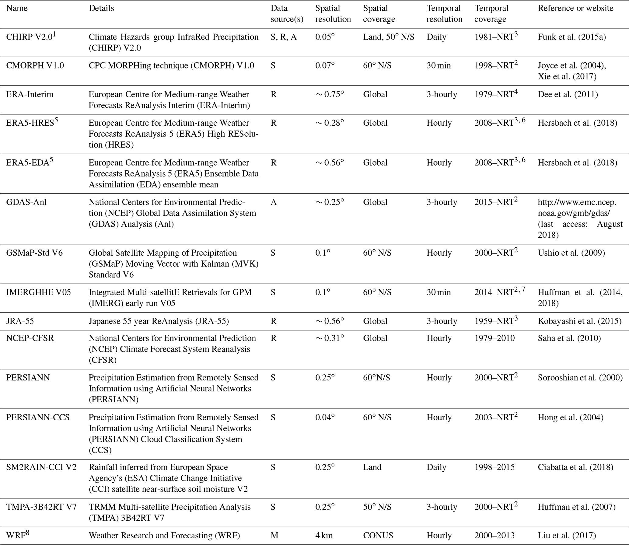
1 The daily variability is based on satellite and reanalysis data. However, the monthly climatology has been corrected using a gauge-based dataset (Funk et al., 2015b). 2 Available until the present with a delay of several hours. 3 Available until the present with a delay of several days. 4 Available until the present with a delay of several months. 5 Rain gauge and ground radar observations were assimilated from 17 July 2009 onwards (Lopez, 2011, 2013). 6 1950–NRT once production has been completed. 7 2000–NRT for the next version. 8 The only dataset included in the evaluation with continental coverage instead of (quasi-)global coverage.
Table 2Overview of the 11 gauge-corrected (quasi-)global (sub-)daily gridded P datasets evaluated in this study. The 15 uncorrected datasets are listed in Table 1. Abbreviations in the data source(s) column defined as G, gauge; S, satellite; R, reanalysis; and A, analysis. The abbreviation NRT in the temporal coverage column stands for near real time. In the spatial coverage column, “global” indicates fully global coverage including ocean areas, while “land” indicates that the coverage is limited to the terrestrial surface.
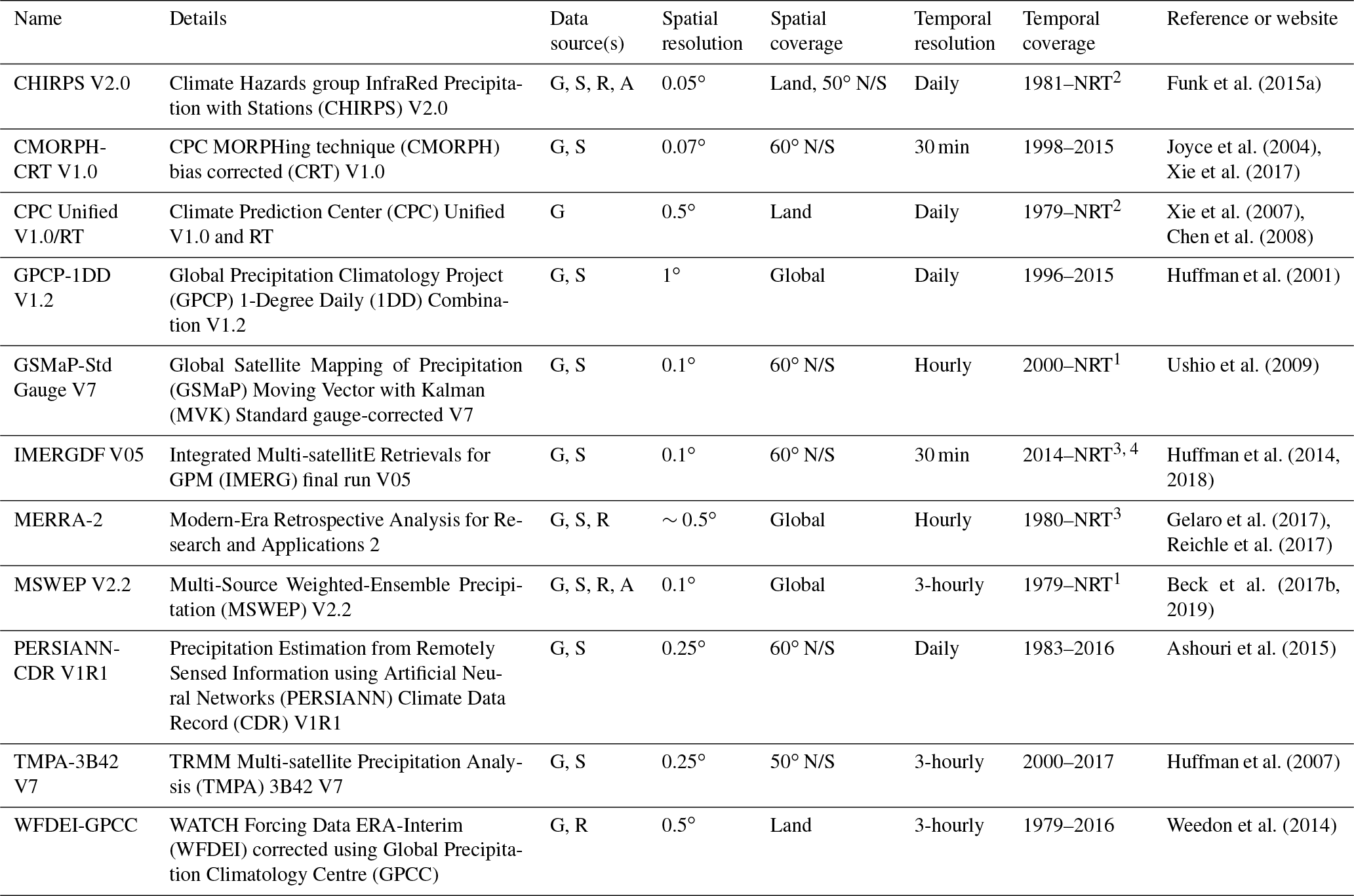
1 Available until the present with a delay of several hours. 2 Available until the
present with a delay of several days. 3 Available until the present with a delay of several months.
4 2000–NRT
for the next version.
2.1 P datasets
We evaluated the performance of 26 gridded (sub-)daily P datasets (Tables 1 and 2). All datasets are either fully or near global, with the exception of WRF, which is limited to the CONUS. The datasets are classified as either uncorrected, which implies that temporal variations depend entirely on satellite and/or (re)analysis data, or corrected, which implies that temporal variations depend to some degree on gauge observations. We included seven datasets exclusively based on satellite data (CMORPH V1.0, GSMaP-Std V6, IMERGHHE V05, PERSIANN, PERSIANN-CCS, SM2RAIN-CCI V2, and TMPA-3B42RT V7), six fully based on (re)analyses (ERA-Interim, ERA5-HRES, ERA5-EDA, GDAS-Anl, JRA-55, and NCEP-CFSR, although ERA5 assimilates radar and gauge data over the CONUS), one incorporating both satellite and (re)analysis data (CHIRP V2.0), and one based on a regional convection-permitting climate model (WRF).
Among the gauge-based P datasets, six combined gauge and satellite data (CMORPH-CRT V1.0, GPCP-1DD V1.2, GSMaP-Std Gauge V7, IMERGDF V05, PERSIANN-CDR V1R1, and TMPA-3B42 V7), one combined gauge and reanalysis data (WFDEI-GPCC), three combined gauge, satellite, and (re)analysis data (CHIRPS V2.0, MERRA-2, and MSWEP V2.2), while one was fully based on gauge observations (CPC Unified V1.0/RT). For transparency and reproducibility, we report dataset version numbers throughout the study for the datasets for which this information was provided. For the P datasets with a sub-daily temporal resolution, we calculated daily accumulations for 00:00–23:59 UTC. P datasets with spatial resolutions <0.1∘ were resampled to 0.1∘ using bilinear averaging, whereas those with spatial resolutions >0.1∘ were resampled to 0.1∘ using bilinear interpolation.
2.2 Stage-IV gauge-radar data
As a reference, we used the NCEP Stage-IV dataset, which has a 4 km spatial and hourly temporal resolution and covers the period 2002 until the present, and merges data from 140 radars and ∼5500 gauges over the CONUS (Lin and Mitchell, 2005). Stage-IV provides highly accurate P estimates and has therefore been widely used as a reference for the evaluation of P datasets (e.g., AghaKouchak et al., 2011, 2012; Habib et al., 2009; Hong et al., 2006; Nelson et al., 2016; Zhang et al., 2018b). Daily Stage-IV data are available, but they represent an accumulation period that is incompatible with the datasets we are evaluating (12:00–11:59 UTC instead of 00:00–23:59 UTC). We therefore calculated daily accumulations for 00:00–23:59 UTC from 6-hourly Stage-IV accumulations. The Stage-IV dataset was reprojected from its native 4 km polar stereographic projection to a regular geographic 0.1∘ grid using bilinear averaging.
The Stage-IV dataset is a mosaic of regional analyses produced by 12 CONUS River Forecast Centers (RFCs) and is thus subject to the gauge correction and quality control performed at each individual RFC (Eldardiry et al., 2017; Smalley et al., 2014; Westrick et al., 1999). To reduce systematic biases, the Stage-IV dataset was rescaled such that its long-term mean matches that of the PRISM dataset (Daly et al., 2008) for the evaluation period (2008–2017). To this end, the PRISM dataset was upscaled from ∼800 m to 0.1∘ using bilinear averaging. The PRISM dataset has been derived from gauge observations using a sophisticated interpolation approach that accounts for topography. It is generally considered the most accurate monthly P dataset available for the US and has been used as a reference in numerous studies (e.g., Liu et al., 2017; Mizukami and Smith, 2012; Prat and Nelson, 2015). However, the dataset has not been corrected for wind-induced gauge undercatch and thus may underestimate P to some degree (Groisman and Legates, 1994; Rasmussen et al., 2012).
2.3 Evaluation approach
The evaluation was performed at a daily temporal and 0.1∘ spatial resolution by calculating, for each grid cell, KGE scores from daily time series for the 10-year period from 2008 to 2017. KGE is an objective performance metric combining correlation, bias, and variability. It was introduced in Gupta et al. (2009) and modified in Kling et al. (2012) and is defined as follows:
where the correlation component r is represented by (Pearson's) correlation coefficient, the bias component β by the ratio of estimated and observed means, and the variability component γ by the ratio of the estimated and observed coefficients of variation:
where μ and σ are the distribution mean and standard deviation, respectively, and the subscripts s and o indicate estimate and reference, respectively. KGE, r, β, and γ values all have their optimum at unity.
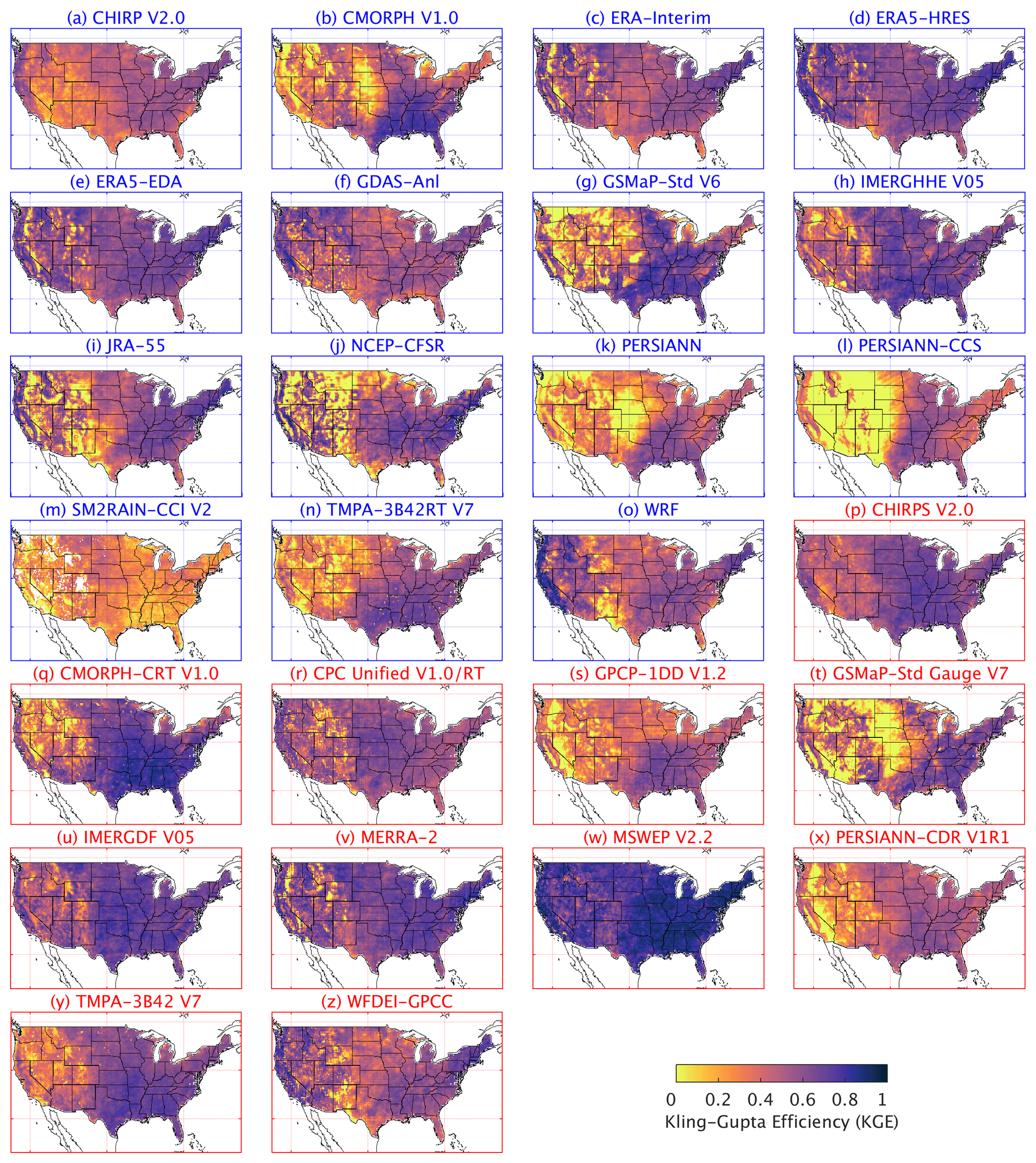
Figure 1KGE scores for the 26 gridded P datasets using the Stage-IV gauge-radar dataset as a reference. White indicates missing data. Higher KGE values correspond to better performance. Uncorrected datasets are listed in blue, whereas gauge-corrected datasets are listed in red. Details on the datasets are provided in Tables 1 and 2. Maps for the correlation, bias, and variability components of the KGE are presented in the Supplement.

Figure 2Box-and-whisker plots of KGE scores for the 26 gridded P datasets using the Stage-IV gauge-radar dataset as a reference. The circles represent the median value, the left and right edges of the box represent the 25th and 75th percentile values, respectively, while the “whiskers” represent the extreme values. The statistics were calculated for each dataset from the distribution of grid-cell KGE values (no area weighting was performed). The datasets are sorted in ascending order of the median KGE. Uncorrected datasets are indicated in blue, whereas gauge-corrected datasets are indicated in red. Details on the datasets are provided in Tables 1 and 2.
3.1 What is the most important factor determining a high KGE score?
Figure 2 presents box-and-whisker plots of KGE scores for the 26 P datasets. The mean median KGE score over all datasets is 0.54. The mean median scores for the correlation, bias, and variability components of the KGE, expressed as , , and , are 0.34, 0.18, and 0.16, respectively (see Eq. 1). The datasets thus performed considerably worse in terms of correlation, which makes sense given that long-term climatological P statistics are easier to estimate than day-to-day P dynamics. Due to the squaring of the three components in the KGE equation (see Eq. 1), the correlation values exert the dominant influence on the final KGE scores. Indeed, the performance ranking in terms of KGE corresponds well to the performance ranking in terms of correlation (Fig. 2). These results suggest that in order to get an improved KGE score, the most important component score to improve is the correlation. This in turn suggests that, for existing daily P datasets, improvements to the timing of P events at the daily scale (dominating the correlation scores) are more valuable than improvements to P totals (dominating bias scores) or the intensity distribution (dominating variability scores).
3.2 How do the uncorrected P datasets perform?
Among the uncorrected P datasets, the (re)analyses performed better overall than the satellite-based datasets (Figs. 1 and 2). The best performance was obtained by ECMWF's fourth-generation reanalysis ERA5-HRES (median KGE of 0.63), with NASA's most recent satellite-based dataset IMERGHHE V05 and the ensemble average ERA5-EDA coming a close equal second (median KGE of 0.62). These results underscore the substantial advances in earth system modeling and satellite-based P estimation over the last decade. The third-generation, coarser-resolution reanalyses (ERA-Interim, JRA-55, and NCEP-CFSR) performed slightly worse overall (median KGE of 0.55, 0.52, and 0.52, respectively). ERA-Interim performed slightly better than other third-generation reanalyses, consistent with earlier studies focusing on P (Beck et al., 2017c; Bromwich et al., 2011; Palerme et al., 2017; Peña Arancibia et al., 2013) and other atmospheric variables (Bracegirdle and Marshall, 2012; Jin-Huan et al., 2014; Zhang et al., 2016). All (re)analyses, including the new ERA5-HRES, underestimated the variability (Figs. 2 and S3 in the Supplement), reflecting the tendency of (re)analyses to overestimate P frequency (Beck et al., 2017c; Lopez, 2007; Skok et al., 2015; Stephens et al., 2010; Sun et al., 2006; Zolina et al., 2004). The additional variability underestimation by ERA5-EDA compared to ERA5-HRES probably reflects the variance loss induced by the averaging.
Among the uncorrected satellite-based P datasets, the new IMERGHHE V05 performed best overall by a substantial margin (median KGE of 0.62; Figs. 1 and 2), reflecting the quality of the new IMERG P retrieval algorithm (Huffman et al., 2014, 2018). The other passive-microwave-based datasets (CMORPH V1.0, GSMaP-Std V6, and TMPA-3B42RT V7) obtained median KGE scores ranging from 0.44 to 0.52. CHIRP V2.0, which combines infrared- and reanalysis-based estimates, performed similarly to some of the passive-microwave datasets (median KGE of 0.47). The datasets exclusively based on infrared data (PERSIANN and PERSIANN-CCS) performed markedly worse (median KGE of 0.34 and 0.32, respectively), consistent with previous P dataset evaluations (e.g., Beck et al., 2017c; Cattani et al., 2016; Hirpa et al., 2010; Peña Arancibia et al., 2013). This has been attributed to the indirect nature of the relationship between cloud-top temperatures and surface rainfall (Adler and Negri, 1988; Scofield and Kuligowski, 2003; Vicente et al., 1998). The infrared-based datasets generally exhibited a much larger spatial variability in performance for all four metrics (Figs. 1 and S1–S3).
The (uncorrected) satellite soil moisture-based SM2RAIN-CCI V2 dataset performed comparatively poorly (median KGE of 0.28; Figs. 1 and 2). The dataset strongly underestimated the variability (Fig. S3), due to the noisiness of satellite soil moisture retrievals and the inability of satellite soil moisture-based algorithms to detect rainfall exceeding the soil water storage capacity (Ciabatta et al., 2018; Tarpanelli et al., 2017; Wanders et al., 2015; Zhan et al., 2015). At high latitudes and elevations, the presence of snow and frozen soils may have hampered performance (Brocca et al., 2014), while in arid regions, irrigation may have been misinterpreted as rainfall (Brocca et al., 2018). In addition, approximately 25 % (in the eastern CONUS) to 50 % (over the mountainous west) of the daily rainfall values were based on temporal interpolation, to fill gaps in the satellite soil moisture data (Dorigo et al., 2017). Despite these limitations, the SM2RAIN datasets may provide new possibilities for evaluation (Massari et al., 2017) and correction (Massari et al., 2018) of other P datasets, since they constitute a fully independent, alternative source of rainfall data.
All uncorrected P datasets exhibited lower overall performance in the western CONUS (Figs. 1, 2, and S1–S3), in line with previous studies (e.g., AghaKouchak et al., 2012; Beck et al., 2017c; Chen et al., 2013; Ebert et al., 2007; Gebregiorgis et al., 2018; Gottschalck et al., 2005; Tian et al., 2007). This is attributable to the more complex topography and greater spatio-temporal heterogeneity of P in the west (Daly et al., 2008), which affects the quality of both the evaluated datasets and the reference (Eldardiry et al., 2017; Smalley et al., 2014; Westrick et al., 1999). With the exception of CHIRP V2.0 (which has been corrected for systematic biases using gauge observations; Funk et al., 2015b) and WRF (the high-resolution climate simulation; Liu et al., 2017), the (uncorrected) datasets exhibited large P biases over the mountainous west (Fig. S2), which is in agreement with earlier studies using other reference datasets (Adam et al., 2006; Beck et al., 2017a, c; Kauffeldt et al., 2013) and reflects the difficulty of retrieving and simulating orographic P (Roe, 2005). We initially expected bias values to be higher than unity since PRISM, the dataset used to correct systematic biases in Stage-IV (see Sect. 2.2), lacks explicit gauge undercatch corrections (Daly et al., 2008), but this did not appear to be the case (Figs. 2 and S2).
3.3 How do the gauge-based P datasets perform?
Among the gauge-based P datasets, the best overall performance was obtained by MSWEP V2.2 (median KGE of 0.81), followed at some distance by IMERGDF V05 (median KGE of 0.67) and MERRA-2 (median KGE of 0.66; Figs. 1 and 2). IMERGDF V05 exhibited a small negative bias, while MERRA-2 slightly underestimated the variability. The good performance obtained by MSWEP V2.2 underscores the importance of incorporating daily gauge data and accounting for reporting times (Beck et al., 2019). While CMORPH-CRT V1.0, CPC Unified V1.0/RT, GSMaP-Std Gauge V7, and MERRA-2 also incorporate daily gauge data, they did not account for reporting times, resulting in temporal mismatches and hence lower KGE scores (Fig. 2). Reporting times in the CONUS range from midnight −12 to +9 h UTC for the stations in the comprehensive GHCN-D gauge database (Menne et al., 2012; Fig. 2c in Beck et al., 2019), suggesting that up to half of the daily P accumulations may be assigned to the wrong day. In addition, CMORPH-CRT V1.0, GSMaP-Std Gauge V7, and MERRA-2 applied daily gauge corrections using CPC Unified (Chen et al., 2008; Xie et al., 2007), which has a relatively coarse 0.5∘ resolution, whereas MSWEP V2.2 applied corrections at 0.1∘ resolution based on the five nearest gauges for each grid cell (Beck et al., 2019). The good performance of IMERGDF V05 is somewhat surprising, given the use of monthly rather than daily gauge data, and attests to the quality of the IMERG P retrieval algorithm (Huffman et al., 2014, 2018).
Similar to the uncorrected datasets, the corrected estimates consistently performed worse in the west (Figs. 1, 2, and S1–S3), due not only to the greater spatio-temporal heterogeneity in P (Daly et al., 2008), but also the lower gauge network density (Kidd et al., 2017). It should be kept in mind that the performance ranking may differ across the globe depending on the amount of gauge data ingested and the quality control applied for each dataset. Thus, the results found here for the CONUS do not necessarily directly generalize to other regions.
3.4 How do the P datasets perform in summer versus winter?
Figure 3 presents KGE values for summer and winter for the 26 P datasets. The following observations can be made.
-
The spread in median KGE values among the datasets is much greater in winter than in summer. In addition, almost all datasets exhibit a greater spatial variability in KGE values in winter, as indicated by the wider boxes and whiskers. This is probably at least partly attributable to the lower quality of the Stage-IV dataset in winter (Eldardiry et al., 2017; Smalley et al., 2014; Westrick et al., 1999).
-
All (re)analyses (with the exception of NCEP-CFSR) including the WRF regional climate model consistently performed better in winter than in summer. This is because predictable large-scale stratiform systems dominate in winter (Adler et al., 2001; Coiffier, 2011; Ebert et al., 2007), whereas unpredictable small-scale convective cells dominate in summer (Arakawa, 2004; Prein et al., 2015).
-
All satellite P datasets (with the exception of PERSIANN) consistently performed better in summer than in winter. Satellites are ideally suited to detect the intense, localized convective storms which dominate in summer (AghaKouchak et al., 2011; Wardah et al., 2008). Conversely, there are major challenges associated with the retrieval of snowfall (Kongoli et al., 2003; Liu and Seo, 2013; Skofronick-Jackson et al., 2015; You et al., 2017) and light rainfall (Habib et al., 2009; Kubota et al., 2009; Lu and Yong, 2018; Tian et al., 2009), affecting the performance in winter.
-
The datasets incorporating both satellite and reanalysis estimates (CHIRP V2.0, CHIRPS V2.0, and MSWEP V2.2) performed similarly in both seasons, taking advantage of the accuracy of satellite retrievals in summer and reanalysis outputs in winter (Beck et al., 2017b; Ebert et al., 2007). The fully gauge-based CPC Unified V1.0/RT also performed similarly in both seasons.
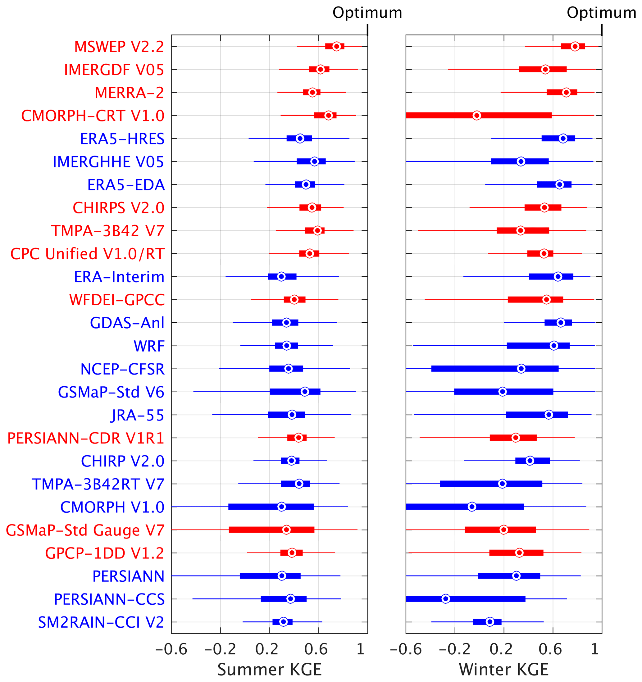
Figure 3Box-and-whisker plots of KGE scores for summer (June–August) and winter (December–February) using the Stage-IV gauge-radar dataset as a reference. The circles represent the median value, the left and right edges of the box represent the 25th and 75th percentile values, respectively, while the “whiskers” represent the extreme values. The statistics were calculated for each dataset from the distribution of grid-cell KGE values (no area weighting was performed). The datasets are sorted in ascending order of the overall median KGE (see Fig. 2). Uncorrected datasets are indicated in blue, whereas gauge-corrected datasets are indicated in red. Details on the datasets are provided in Tables 1 and 2.
3.5 What is the impact of gauge corrections?
Differences in median KGE values between uncorrected and gauge-corrected versions of P datasets ranged from −0.07 (GSMaP-Std Gauge V7) to +0.20 (CMORPH-CRT V1.0; Table 3). GSMaP-Std Gauge V7 shows a large positive bias in the west (Fig. S2), suggesting that its gauge-correction methodology requires re-evaluation. The substantial improvements in median KGE for CHIRPS V2.0 (+0.13) and CMORPH-CRT V1.0 (+0.20) reflect the use of sub-monthly gauge data (5-day and daily, respectively). Conversely, the datasets incorporating monthly gauge data (IMERGDF V05 and WFDEI-GPCC) exhibited little to no improvement in median KGE (+0.05 and −0.01, respectively), suggesting that monthly corrections provide little to no benefit at the daily timescale of the present evaluation (Tan and Santo, 2018). These results, combined with the fact that several uncorrected P datasets outperformed gauge-corrected ones (Fig. 2), suggest that a P dataset labeled as “gauge-corrected” is not necessarily always the better choice.

Figure 4(a) KGE scores obtained by IMERGHHE V05 minus those obtained by TMPA-3B42RT V7. (b) KGE scores obtained by ERA5-HRES minus those obtained by ERA-Interim. (c) Correlations (r) obtained by ERA5-EDA minus those obtained by ERA5-HRES. (d) KGE scores obtained by IMERGHHE V05 minus those obtained by ERA5-HRES. Note the different color scales. The Stage-IV gauge-radar dataset was used as a reference. The KGE and correlation values were calculated from daily time series.

3.6 What is the improvement of IMERG over TMPA?
IMERG (Huffman et al., 2014, 2018) is NASA's latest satellite P dataset and is foreseen to replace the TMPA dataset (Huffman et al., 2007; Table 1). The following main improvements were implemented in IMERG compared to TMPA: (i) forward and backward propagation of passive microwave data using CMORPH-style motion vectors (Joyce et al., 2004); (ii) infrared-based rainfall estimates derived using the PERSIANN-CCS algorithm (Hong et al., 2004); (iii) calibration of passive microwave-based P estimates to the Combined GMI-DPR P dataset (available up to almost 70∘ latitude) during the GPM era and the Combined TMI-PR P dataset (available up to 40∘ latitude) during the TRMM era; (iv) adjustment of the Combined estimates by GPCP monthly climatological values (Adler et al., 2018) to ameliorate low biases at high latitudes; (v) merging of infrared- and passive microwave-based P estimates using a CMORPH-style Kalman filter; (vi) use of passive microwave data from recent instruments (DMSP-F19, GMI, and NOAA-20); (vii) a 30 min temporal resolution (instead of 3-hourly); (viii) a 0.1∘ spatial resolution (instead of 0.25∘); and (ix) greater coverage (essentially complete up to 60∘ instead of 50∘ latitude).
These changes have resulted in considerable performance improvements: IMERGHH V05 performed better overall than TMPA-3B42RT V7 in terms of median KGE (0.62 versus 0.46), correlation (0.69 versus 0.59), bias (0.99 versus 1.09), and variability (1.05 versus 1.07; Figs. 1, 2, and 4a). The improvement is particularly pronounced over the northern Great Plains (Fig. 4a), where TMPA-3B42RT V7 exhibits a large positive bias (Fig. S2). In the west, however, there are still some small regions over which TMPA-3B42RT V7 performed better (Fig. 4a). Overall, our results indicate that there is considerable merit in using IMERGHHE V05 instead of TMPA-3B42RT V7 over the CONUS. Previous studies comparing (different versions of) the same two datasets over the CONUS (Gebregiorgis et al., 2018), Bolivia (Satgé et al., 2017), mainland China (Tang et al., 2016a), southeast China (Tang et al., 2016b), Iran (Sharifi et al., 2016), India (Prakash et al., 2016), the Mekong River basin (Wang et al., 2017), the Tibetan Plateau (Ran et al., 2017), and the northern Andes (Manz et al., 2017) reached largely similar conclusions.
3.7 What is the improvement of ERA5 over ERA-Interim?
ERA5 (Hersbach et al., 2018) is ECMWF's recently released fourth-generation reanalysis and the successor to ERA-Interim, generally considered the most accurate third-generation reanalysis (Beck et al., 2017c; Bracegirdle and Marshall, 2012; Bromwich et al., 2011; Jin-Huan et al., 2014; Table 1). ERA5 features several improvements over ERA-Interim, such as (i) a more recent model and data assimilation system (IFS Cycle 41r2 from 2016 versus IFS Cycle 31r2 from 2006), including numerous improvements in model physics, numerics, and data assimilation; (ii) a higher horizontal resolution (∼0.28∘ versus ∼0.75∘); (iii) more vertical levels (137 versus 60); (iv) assimilation of substantially more observations, including gauge (Lopez, 2013) and ground radar (Lopez, 2011) P data (from 17 July 2009 onwards); (v) a longer temporal span once production has completed (1950–present versus 1979–present) and a near-real-time release of the data; (vi) outputs with a higher temporal resolution (hourly versus 3-hourly); and (vii) corresponding uncertainty estimates.
As a result of these changes ERA5-HRES performed markedly better than ERA-Interim in terms of P across most of the CONUS, especially in the west (Figs. 1 and 4b). ERA5-HRES obtained a median KGE of 0.63, whereas ERA-Interim obtained a median KGE of 0.55 (Fig. 2). Improvements were evident for all three KGE components (correlation, bias, and variability). It is difficult to say how much of the performance improvement of ERA5 is due to the assimilation of gauge and radar P data. We suspect that the performance improvement is largely attributable to other factors, given that (i) the impact of the P data assimilation is limited overall due to the large amount of other observations already assimilated (Lopez, 2013); (ii) radar data were discarded west of 105∘ W for quality reasons (Lopez, 2011); and (iii) performance improvements were also found in regions without assimilated gauge observations (e.g., Nevada; Fig. 4b; Lopez, 2013, their Fig. 3). Nevertheless, we expect the performance difference between ERA5 and ERA-Interim to be less in regions with fewer or no assimilated gauge observations (i.e., outside the US, Canada, Argentina, Europe, Iran, and China; Lopez, 2013, their Fig. 3).
So far, only three other studies have compared the performance of ERA5 and ERA-Interim. The first study compared the two reanalyses for the CONUS by using them to drive a land surface model (Albergel et al., 2018). The simulations using ERA5 provided substantially better evaporation, soil moisture, river discharge, and snow depth estimates. The authors attributed this to the improved P estimates, which is supported by our results. The second and third studies evaluated incoming shortwave radiation and precipitable water vapor estimates from the two reanalyses, respectively, with both studies reporting that ERA5 provides superior performance (Urraca et al., 2018; Zhang et al., 2018a).
3.8 How does the ERA5-EDA ensemble average compare to the ERA5-HRES deterministic run?
Ensemble modeling involves using outputs from multiple models or from different realizations of the same model; it is widely used in climate, atmospheric, hydrological, and ecological sciences to improve accuracy and quantify uncertainty (Beck et al., 2013, 2017a; Cheng et al., 2012; Gneiting and Raftery, 2005; Nikulin et al., 2012; Strauch et al., 2012). Here, we compare the P estimation performance of a high-resolution (∼0.28∘) deterministic reanalysis (ERA5-HRES) to that of a reduced-resolution (∼0.56∘) ensemble average (ERA5-EDA; Table 1). The ensemble consists of 10 members generated by perturbing the assimilated observations (Zuo et al., 2017) as well as the model physics (Leutbecher et al., 2017; Ollinaho et al., 2016). The ensemble average was derived by equal weighting of the members.
Compared to ERA5-HRES, we found ERA5-EDA to perform similarly in terms of median KGE (0.62 versus 0.63), better in terms of median correlation (0.72 versus 0.69) and bias (0.96 versus 0.93), but worse in terms of median variability (0.80 versus 0.90; Figs. 1, 2, and 4c). The deterioration of the variability is probably at least partly due to the averaging, which shifts the distribution toward medium-sized events. The improvement in correlation is evident over the entire CONUS (Fig. 4c), and corresponds to a 9 % overall increase in the explained temporal variance, demonstrating the value of ensemble modeling. We expect the improvement to increase with increasing diversity among ensemble members (Brown et al., 2005; DelSole et al., 2014).
3.9 How do IMERG and ERA5 compare?
IMERGHHE V05 (Huffman et al., 2014, 2018) and ERA5-HRES (Hersbach et al., 2018) represent the state-of-the-art in terms of satellite P retrieval and reanalysis, respectively (Table 1). Although the datasets exhibited similar performance overall (median KGE of 0.62 and 0.63, respectively; Figs. 1 and 2), regionally there were considerable differences (Fig. 4d). Compared to ERA5-HRES, IMERGHHE V05 performed substantially worse over regions of complex terrain (including the Rockies and the Appalachians), in line with previous evaluations focusing on India (Prakash et al., 2018) and western Washington state (Cao et al., 2018). In contrast, ERA5-HRES performed worse across the southern–central US, where P predominantly originates from small-scale, short-lived convective storms which tend to be poorly simulated by reanalyses (Adler et al., 2001; Arakawa, 2004; Ebert et al., 2007). The patterns in relative performance between IMERGHHE V05 and ERA5-HRES (Fig. 4d) correspond well to those found between TMPA 3B42RT and ERA-Interim (Beck et al., 2017b, their Fig. 4) and between CMORPH and ERA-Interim (Beck et al., 2019, their Fig. 3d), suggesting that our conclusions can be generalized to other satellite- and reanalysis-based P datasets. Our findings suggest that topography and climate should be taken into account when choosing between satellite and reanalysis datasets. Furthermore, our results demonstrate the potential to improve continental- and global-scale P datasets by merging satellite- and reanalysis-based P estimates (Beck et al., 2017b, 2019; Huffman et al., 1995; Sapiano et al., 2008; Xie and Arkin, 1996; Zhang et al., 2018b).
3.10 How well does a regional convection-permitting climate model perform?
In addition to the (quasi-)global P datasets, we evaluated the performance of a state-of-the-art climate simulation for the CONUS (WRF; Liu et al., 2017; Table 1). The WRF simulation has the potential to produce highly accurate P estimates since it has a high 4 km resolution, which allows it to account for the influence of mesoscale orography (Doyle, 1997), and is “convection-permitting”, which means it does not rely on highly uncertain convection parameterizations (Kendon et al., 2012; Prein et al., 2015). In terms of variability, WRF performed third best, being outperformed only (and very modestly) by the gauge-based CPC Unified V1.0/RT and MSWEP V2.2 datasets (Figs. 1 and 2). In terms of bias, the simulation produced mixed results. WRF is the only uncorrected dataset that does not exhibit large biases over the mountainous west (Fig. S2). However, large positive biases were obtained over the Great Plains region, as also found by Liu et al. (2017) using the same reference data. In terms of correlation, WRF performed worse than third-generation reanalyses (ERA-Interim, JRA-55, and NCEP-CFSR; Figs. 2 and S1). This is probably because WRF is forced entirely by lateral and initial boundary conditions from ERA-Interim (Liu et al., 2017), whereas the reanalyses assimilate vast amounts of in situ and satellite observations (Dee et al., 2011; Kobayashi et al., 2015; Saha et al., 2010). Overall, there appears to be some merit in using high-resolution, convection-permitting models to obtain climatological P statistics.
To shed some light on the strengths and weaknesses of different precipitation (P) datasets and on the merit of different technological and methodological innovations, we comprehensively evaluated the performance of 26 gridded (sub-)daily P datasets for the CONUS using Stage-IV gauge-radar data as a reference. The evaluation was carried out at a daily temporal and 0.1∘ spatial scale for the period 2008–2017 using the KGE, an objective performance metric combining correlation, bias, and variability. Our findings can be summarized as follows.
-
Across the range of KGE scores for the datasets examined the most important component is correlation (reflecting the identification of P events). Of secondary importance are the P totals (determining the bias score) and the distribution of P intensity (affecting the variability score).
-
Among the uncorrected P datasets, the (re)analyses performed better on average than the satellite-based datasets. The best performance was obtained by ECMWF's fourth-generation reanalysis ERA5-HRES, with NASA's most recent satellite-derived IMERGHHE V05 and the ensemble average ERA5-EDA coming a close equal second.
-
Among the gauge-based P datasets, the best overall performance was obtained by MSWEP V2.2, followed by IMERGDF V05 and MERRA-2. The good performance of MSWEP V2.2 highlights the importance of incorporating daily gauge observations and accounting for gauge reporting times.
-
The spread in performance among the P datasets was greater in winter than in summer. The spatial variability in performance was also greater in winter for most datasets. The (re)analyses generally performed better in winter than in summer, while the opposite was the case for the satellite-based datasets.
-
The performance improvement gained after applying gauge corrections differed strongly among P datasets. The largest improvements were obtained by the datasets incorporating sub-monthly gauge data (CHIRPS V2.0 and CMORPH-CRT V1.0). Several uncorrected P datasets outperformed gauge-corrected ones.
-
IMERGHH V05 performed better than TMPA-3B42RT V7 for all metrics, consistent with previous studies and attributable to the many improvements implemented in the new IMERG algorithm.
-
ERA5-HRES outperformed ERA-Interim for all metrics across most of the CONUS, demonstrating the significant advances in climate and earth system modeling and data assimilation during the last decade.
-
The reduced-resolution ERA5-EDA ensemble average showed higher correlations than the high-resolution ERA5-HRES deterministic run, supporting the value of ensemble modeling. However, a side effect of the averaging is that the P distribution shifted toward medium-sized events.
-
IMERGHHE V05 and ERA5-HRES showed complementary performance patterns. The former performed substantially better in regions dominated by convective storms, while the latter performed substantially better in regions of complex terrain.
-
Regional convection-permitting climate model WRF performed best among the uncorrected P datasets in terms of variability. This suggests there is some merit in employing high-resolution, convection-permitting models to obtain climatological P statistics.
Our findings provide some guidance to decide which P dataset should be used for a particular application. We found evidence that the relative performance of different datasets is to some degree a function of topographic complexity, climate regime, season, and rain gauge network density. Therefore, care should be taken when extrapolating our results to other regions. Additionally, results may differ when using another performance metric or when evaluating other timescales or aspects of the datasets. Similar evaluations should be carried out with other performance metrics and in other regions with ground radar networks (e.g., Australia and Europe) to verify and supplement the present findings. Of particular importance in the context of climate change is the further evaluation of P extremes.
The P datasets are available via the respective websites of the dataset producers.
The supplement related to this article is available online at: https://doi.org/10.5194/hess-23-207-2019-supplement.
HB conceived the study, performed the analysis, and wrote the paper. The other authors commented on the paper and helped with the writing.
The authors declare that they have no conflict of interest.
We gratefully acknowledge the P dataset developers for producing and making
available their datasets. We thank Marie-Claire ten Veldhuis, Dick Dee, Christa Peters-Lidard, Jelle ten Harkel, Luca Brocca, and an anonymous
reviewer for their
thoughtful evaluation of the manuscript. Hylke E. Beck was supported through
IPA support from the U.S. Army Corps of Engineers' International Center for
Integrated Water Resources Management (ICIWaRM), under the auspices of
UNESCO. Graham P. Weedon was supported by the Joint DECC and Defra
Integrated Climate Program – DECC/Defra (GA01101).
Edited by: Marie-Claire ten Veldhuis
Reviewed by: Dick Dee and one anonymous referee
Adam, J. C., Clark, E. A., Lettenmaier, D. P., and Wood, E. F.: Correction of global precipitation products for orographic effects, J. Climate, 19, 15–38, https://doi.org/10.1175/JCLI3604.1, 2006. a
Adler, R. F. and Negri, A. J.: A satellite infrared technique to estimate tropical convective and stratiform rainfall, J. Appl. Meteorol., 27, 30–51, 1988. a
Adler, R. F., Kidd, C., Petty, G., Morissey, M., and Goodman, H. M.: Intercomparison of global precipitation products: The third precipitation intercomparison project (PIP-3), B. Am. Meteorol. Soc., 82, 1377–1396, 2001. a, b
Adler, R. F., Sapiano, M. R. P., Huffman, G. J., Wang, J.-J., Gu, G., Bolvin, D., Chiu, L., Schneider, U., Becker, A., Nelkin, E., Xie, P., Ferraro, R., and Shin, D.-B.: The Global Precipitation Climatology Project (GPCP) monthly analysis (new version 2.3) and a review of 2017 global precipitation, Atmosphere, 9, 138, https://doi.org/10.3390/atmos9040138, 2018. a
AghaKouchak, A., Behrangi, A., Sorooshian, S., Hsu, K., and Amitai, E.: Evaluation of satellite retrieved extreme precipitation rates across the central United States, J. Geophys. Res.-Atmos., 116, https://doi.org/10.1029/2010JD014741, 2011. a, b
AghaKouchak, A., Mehran, A., Norouzi, H., and Behrangi, A.: Systematic and random error components in satellite precipitation data sets, Geophys. Res. Lett., 39, https://doi.org/10.1029/2012GL051592, 2012. a, b
Albergel, C., Dutra, E., Munier, S., Calvet, J.-C., Munoz-Sabater, J., de Rosnay, P., and Balsamo, G.: ERA-5 and ERA-Interim driven ISBA land surface model simulations: which one performs better?, Hydrol. Earth Syst. Sci., 22, 3515–3532, https://doi.org/10.5194/hess-22-3515-2018, 2018. a
Arakawa, A.: The cumulus parameterization problem: past, present, and future, J. Climate, 17, 2493–2525, 2004. a, b
Ashouri, H., Hsu, K., Sorooshian, S., Braithwaite, D. K., Knapp, K. R., Cecil, L. D., Nelson, B. R., and Pratt, O. P.: PERSIANN-CDR: daily precipitation climate data record from multisatellite observations for hydrological and climate studies, B. Am. Meteorol. Soc., 96, 69–83, 2015. a
Beck, H. E., van Dijk, A. I. J. M., Miralles, D. G., de Jeu, R. A. M., Bruijnzeel, L. A., McVicar, T. R., and Schellekens, J.: Global patterns in baseflow index and recession based on streamflow observations from 3394 catchments, Water Resour. Res., 49, 7843–7863, 2013. a
Beck, H. E., van Dijk, A. I. J. M., de Roo, A., Dutra, E., Fink, G., Orth, R., and Schellekens, J.: Global evaluation of runoff from 10 state-of-the-art hydrological models, Hydrol. Earth Syst. Sci., 21, 2881–2903, https://doi.org/10.5194/hess-21-2881-2017, 2017a. a, b
Beck, H. E., van Dijk, A. I. J. M., Levizzani, V., Schellekens, J., Miralles, D. G., Martens, B., and de Roo, A.: MSWEP: 3-hourly 0.25∘ global gridded precipitation (1979–2015) by merging gauge, satellite, and reanalysis data, Hydrol. Earth Syst. Sci., 21, 589–615, https://doi.org/10.5194/hess-21-589-2017, 2017b. a, b, c, d
Beck, H. E., Vergopolan, N., Pan, M., Levizzani, V., van Dijk, A. I. J. M., Weedon, G. P., Brocca, L., Pappenberger, F., Huffman, G. J., and Wood, E. F.: Global-scale evaluation of 22 precipitation datasets using gauge observations and hydrological modeling, Hydrol. Earth Syst. Sci., 21, 6201–6217, https://doi.org/10.5194/hess-21-6201-2017, 2017c. a, b, c, d, e, f, g, h
Beck, H. E., Wood, E. F., Pan, M., Fisher, C. K., Miralles, D. M., van Dijk, A. I. J. M., McVicar, T. R., and Adler, R. F.: MSWEP V2 global 3-hourly 0.1∘ precipitation: methodology and quantitative assessment, B. Am. Meteorol. Soc., in press, https://doi.org/10.1175/BAMS-D-17-0138.1, 2019. a, b, c, d, e, f
Bracegirdle, T. J. and Marshall, G. J.: The reliability of Antarctic tropospheric pressure and temperature in the latest global reanalyses, J. Climate, 25, 7138–7146, 2012. a, b
Brocca, L., Ciabatta, L., Massari, C., Moramarco, T., Hahn, S., Hasenauer, S., Kidd, R., Dorigo, W., Wagner, W., and Levizzani, V.: Soil as a natural rain gauge: estimating global rainfall from satellite soil moisture data, J. Geophys. Res.-Atmos., 119, 5128–5141, 2014. a
Brocca, L., Tarpanelli, A., Filippucci, P., Dorigo, W., Zaussinger, F., Gruber, A., and Fernández-Prieto, D.: How much water is used for irrigation? A new approach exploiting coarse resolution satellite soil moisture products, Int. J. Appl. Earth Obs., 73, 752–766, https://doi.org/10.1016/j.jag.2018.08.023, 2018. a
Bromwich, D. H., Nicolas, J. P., and Monaghan, A. J.: An assessment of precipitation changes over Antarctica and the Southern Ocean since 1989 in contemporary global reanalyses, J. Climate, 24, 4189–4209, 2011. a, b
Brown, G., Wyatt, J. L., and Tin̆o, P.: Managing Diversity in Regression Ensembles, J. Mach. Learn. Res., 6, 1621–1650, 2005. a
Cao, Q., Painter, T. H., Currier, W. R., Lundquist, J. D., and Lettenmaier, D. P.: Estimation of Precipitation over the OLYMPEX Domain during Winter 2015/16, J. Hydrometeorol., 19, 143–160, 2018. a
Cattani, E., Merino, A., and Levizzani, V.: Evaluation of monthly satellite-derived precipitation products over East Africa, J. Hydrometeorol., 17, 2555–2573, 2016. a
Chen, M., Shi, W., Xie, P., Silva, V. B. S., Kousky, V. E., Higgins, R. W., and Janowiak, J. E.: Assessing objective techniques for gauge-based analyses of global daily precipitation, J. Geophys. Res., 113, D04110, https://doi.org/10.1029/2007JD009132, 2008. a, b
Chen, S., Hong, Y., Gourley, J. J., Huffman, G. J., Tian, Y., Cao, Q., Yong, B., Kirstetter, P.-E., Hu, J., Hardy, J., Li, Z., Khan, S. I., and Xue, X.: Evaluation of the successive V6 and V7 TRMM multisatellite precipitation analysis over the Continental United States, Water Resour. Res., 49, https://doi.org/10.1002/2012WR012795, 2013. a
Cheng, S., Li, L., Chen, D., and Li, J.: A neural network based ensemble approach for improving the accuracy of meteorological fields used for regional air quality modeling, J. Environ. Manage., 112, 404–414, https://doi.org/10.1016/j.jenvman.2012.08.020, 2012. a
Ciabatta, L., Massari, C., Brocca, L., Gruber, A., Reimer, C., Hahn, S., Paulik, C., Dorigo, W., Kidd, R., and Wagner, W.: SM2RAIN-CCI: a new global long-term rainfall data set derived from ESA CCI soil moisture, Earth Syst. Sci. Data, 10, 267–280, https://doi.org/10.5194/essd-10-267-2018, 2018. a, b
Coiffier, J.: Fundamentals of Numerical Weather Prediction, Cambridge University Press, Cambridge, UK, 2011. a
Daly, C., Halbleib, M., Smith, J. I., Gibson, W. P., Doggett, M. K., Taylor, G. H., Curtis, J., and Pasteris, P. P.: Physiographically sensitive mapping of climatological temperature and precipitation across the conterminous United States, Int. J. Climatol., 28, 2031–2064, 2008. a, b, c, d
Dee, D. P., Uppala, S. M., Simmons, A. J., Berrisford, P., Poli, P., Kobayashi, S., Andrae, U., Balmaseda, M. A., Balsamo, G., Bauer, P., Bechtold, P., Beljaars, A. C. M., van de Berg, L., Bidlot, J., Bormann, N., Delsol, C., Dragani, R., Fuentes, M., Geer, A. J., Haimberger, L., Healy, S. B., Hersbach, H., Hólm, E. V., Isaksen, L., Kallberg, P., Köhler, M., Matricardi, M., McNally, A. P., Monge-Sanz, B. M., Morcrette, J.-J., Park, B.-K., Peubey, C., de Rosnay, P., Tavolato, C., Thépaut, J.-N., and Vitart, F.: The ERA-Interim reanalysis: configuration and performance of the data assimilation system, Q. J. Roy. Meteor. Soc., 137, 553–597, 2011. a, b
DelSole, T., Nattala, J., and Tippett, M. K.: Skill improvement from increased ensemble size and model diversity, Geophys. Res. Lett., 41, 7331–7342, 2014. a
Dorigo, W., Wagner, W., Albergel, C., Albrecht, F., Balsamo, G., Brocca, L., Chung, D., Ert, M., Forkel, M., Gruber, A., Haas, E., Hamer, P. D., Hirschi, M., Ikonen, J., de Jeu, R., Kidd, R., Lahoz, W., Liu, Y. Y., Miralles, D., Mistelbauer, T., Nicolai-Shaw, N., Parinussa, R., Pratola, C., Reimerak, C., van der Schalie, R., Seneviratne, S. I., Smolander, T., and Lecomte, P.: ESA CCI Soil Moisture for improved Earth system understanding: State-of-the art and future directions, Remote Sens. Environ., 203, 185–215, https://doi.org/10.1016/j.rse.2017.07.001, 2017. a
Doyle, J. D.: The Influence of Mesoscale Orography on a Coastal Jet and Rainband, Mon. Weather Rev., 125, 1465–1488, 1997. a
Ebert, E. E., Janowiak, J. E., and Kidd, C.: Comparison of near-real-time precipitation estimates from satellite observations and numerical models, B. Am. Meteorol. Soc., 88, 47–64, 2007. a, b, c, d, e
Eldardiry, H., Habib, E., Zhang, Y., and Graschel, J.: Artifacts in Stage IV NWS real-time multisensor precipitation estimates and impacts on identification of maximum series, J. Hydrol. Eng., 22, E4015003, https://doi.org/10.1061/(ASCE)HE.1943-5584.0001291, 2017. a, b, c
Funk, C., Peterson, P., Landsfeld, M., Pedreros, D., Verdin, J., Shukla, S., Husak, G., Rowland, J., Harrison, L., Hoell, A., and Michaelsen, J.: The climate hazards infrared precipitation with stations – a new environmental record for monitoring extremes, Scientific Data, 2, 150066, https://doi.org/10.1038/sdata.2015.66, 2015a. a, b, c
Funk, C., Verdin, A., Michaelsen, J., Peterson, P., Pedreros, D., and Husak, G.: A global satellite-assisted precipitation climatology, Earth Syst. Sci. Data, 7, 275–287, https://doi.org/10.5194/essd-7-275-2015, 2015b. a, b
Gebregiorgis, A. S., Kirstetter, P.-E., Hong, Y. E., Gourley, J. J., Huffman, G. J., Petersen, W. A., Xue, X., and Schwaller, M. R.: To what extent is the day 1 GPM IMERG satellite precipitation estimate improved as compared to TRMM TMPA-RT?, J. Geophys. Res.-Atmos., 123, 1694–1707, 2018. a, b
Gebremichael, M.: Framework for satellite rainfall product evaluation, in: Rainfall: State of the Science, edited by: Testik, F. Y. and Gebremichael, M., Geophysical Monograph Series, American Geophysical Union, Washington, D.C., https://doi.org/10.1029/2010GM000974, 2010. a
Gelaro, R., McCarty, W., Suárez, M. J., Todling, R., Molod, A., Takacs, L., Randles, C. A., Darmenov, A., Bosilovich, M. G., Reichle, R., Wargan, K., Coy, L., Cullather, R., Draper, C., Akella, S., Buchard, V., Conaty, A., da Silva, A. M., Gu, W., Kim, G.-K., Koster, R., Lucchesi, R., Merkova, D., Nielsen, J. E., Partyka, G., Pawson, S., Putman, W., Rienecker, M., Schubert, S. D., Sienkiewicz, M., and Zhao, N.: The Modern-Era Retrospective Analysis for Research and Applications, Version 2 (MERRA-2), J. Climate, 30, 5419–5454, 2017. a, b
Gneiting, T. and Raftery, A. E.: Weather Forecasting with Ensemble Methods, Science, 310, 248–249, 2005. a
Gottschalck, J., Meng, J., Rodell, M., and Houser, P.: Analysis of Multiple Precipitation Products and Preliminary Assessment of Their Impact on Global Land Data Assimilation System Land Surface States, J. Hydrometeorol., 6, 573–598, 2005. a
Groisman, P. Y. and Legates, D. R.: The accuracy of United States precipitation data, B. Am. Meteorol. Soc., 72, 215–227, 1994. a
Gupta, H. V., Kling, H., Yilmaz, K. K., and Martinez, G. F.: Decomposition of the mean squared error and NSE performance criteria: Implications for improving hydrological modelling, J. Hydrol., 370, 80–91, 2009. a, b
Habib, E., Henschke, A., and Adler, R. F.: Evaluation of TMPA satellite-based research and real-time rainfall estimates during six tropical-related heavy rainfall events over Louisiana, USA, Atmos. Res., 94, 373–388, 2009. a, b
Herold, N., Alexander, L. V., Donat, M. G., Contractor, S., and Becker, A.: How much does it rain over land?, Geophys. Res. Lett., 43, 341–348, 2016. a
Hersbach, H., de Rosnay, P., Bell, B., Schepers, D., Simmons, A., Soci, C., Abdalla, S., Alonso-Balmaseda, M., Balsamo, G., Bechtold, P., Berrisford, P., Bidlot, J.-R., de Boisséson, E., Bonavita, M., Browne, P., Buizza, R., Dahlgren, P., Dee, D., Dragani, R., Diamantakis, M., Flemming, J., Forbes, R., Geer, A. J., Haiden, T., Hólm, E., Haimberger, L., Hogan, R., Horányi, A., Janiskova, M., Laloyaux, P., Lopez, P., Muñoz-Sabater, J., Peubey, C., Radu, R., Richardson, D., Thépaut, J.-N., Vitart, F., Yang, X., Zsótér, E., and Zuo, H.: Operational global reanalysis: progress, future directions and synergies with NWP, ERA Report Series 27, ECMWF, Reading, UK, 2018. a, b, c, d, e
Hirpa, F. A., Gebremichael, M., and Hopson, T.: Evaluation of high-resolution satellite precipitation products over very complex terrain in Ethiopia, J. Appl. Meteorol. Clim., 49, 1044–1051, 2010. a
Hong, Y., Hsu, K.-L., Sorooshian, S., and Gao, X.: Precipitation Estimation from Remotely Sensed Imagery Using an Artificial Neural Network Cloud Classification System, J. Appl. Meteorol., 43, 1834–1853, 2004. a, b
Hong, Y., Hsu, K., Moradkhani, H., and Sorooshian, S.: Uncertainty quantification of satellite precipitation estimation and Monte Carlo assessment of the error propagation into hydrologic response, Water Resour. Res., 42, https://doi.org/10.1029/2005WR004398, 2006. a
Huffman, G. J., Adler, R. F., Rudolf, B., Schneider, U., and Keehn, P. R.: Global precipitation estimates based on a technique for combining satellite-based estimates, rain gauge analysis, and NWP model precipitation information, J. Climate, 8, 1284–1295, 1995. a, b
Huffman, G. J., Adler, R. F., Morrissey, M. M., Bolvin, D. T., Curtis, S., Joyce, R., McGavock, B., and Susskind, J.: Global precipitation at one-degree daily resolution from multi-satellite observations, J. Hydrometeorol., 2, 36–50, 2001. a
Huffman, G. J., Bolvin, D. T., Nelkin, E. J., Wolff, D. B., Adler, R. F., Gu, G., Hong, Y., Bowman, K. P., and Stocker, E. F.: The TRMM Multisatellite Precipitation Analysis (TMPA): quasi-global, multiyear, combined-sensor precipitation estimates at fine scales, J. Hydrometeorol., 8, 38–55, 2007. a, b, c
Huffman, G. J., Bolvin, D. T., Braithwaite, D., Hsu, K., Joyce, R., Kidd, C., Nelkin, E. J., and Xie, P.: NASA Global Precipitation Measurement (GPM) Integrated Multi-satellitE Retrievals for GPM (IMERG), Algorithm Theoretical Basis Document (ATBD), NASA/GSFC, Greenbelt, MD 20771, USA, 2014. a, b, c, d, e, f, g
Huffman, G. J., Bolvin, D. T., and Nelkin, E. J.: Integrated Multi-satellitE Retrievals for GPM (IMERG) Technical Documentation, Tech. rep., NASA/GSFC, Greenbelt, MD 20771, USA, 2018. a, b, c, d, e, f, g, h
Jin-Huan, Z., Shu-Po, M., Han, Z., Li-Bo, Z., and Peng, L.: Evaluation of reanalysis products with in situ GPS sounding observations in the Eastern Himalayas, Atmos. Oceanic Sci. Lett., 7, 17–22, 2014. a, b
Joyce, R. J., Janowiak, J. E., Arkin, P. A., and Xi, P.: CMORPH: A method that produces global precipitation estimates from passive microwave and infrared data at high spatial and temporal resolution, J. Hydrometeorol., 5, 487–503, 2004. a, b, c
Kauffeldt, A., Halldin, S., Rodhe, A., Xu, C.-Y., and Westerberg, I. K.: Disinformative data in large-scale hydrological modelling, Hydrol. Earth Syst. Sci., 17, 2845–2857, https://doi.org/10.5194/hess-17-2845-2013, 2013. a
Kendon, E. J., Roberts, N. M., Senior, C. A., and Roberts, M. J.: Realism of Rainfall in a Very High-Resolution Regional Climate Model, J. Climate, 25, 5791–5806, 2012. a
Kidd, C., Becker, A., Huffman, G. J., Muller, C. L., Joe, P., Skofronick-Jackson, G., and Kirschbaum, D. B.: So, how much of the Earth's surface is covered by rain gauges?, B. Am. Meteorol. Soc., 98, 69–78, 2017. a
Kirschbaum, D. B., Huffman, G. J., Adler, R. F., Braun, S., Garrett, K., Jones, E., McNally, A., Skofronick-Jackson, G., Stocker, E., Wu, H., and Zaitchik, B. F.: NASA's Remotely Sensed Precipitation: A Reservoir for Applications Users, B. Am. Meteorol. Soc., 98, 1169–1184, 2017. a
Kling, H., Fuchs, M., and Paulin, M.: Runoff conditions in the upper Danube basin under an ensemble of climate change scenarios, J. Hydrol., 424–425, 264–277, https://doi.org/10.1016/j.hydrol.2012.01.011, 2012. a, b
Kobayashi, S., Ota, Y., Harada, Y., Ebita, A., Moriya, M., Onoda, H., Onogi, K., Kamahori, H., Kobayashi, C., Endo, H., Miyaoka, K., and Takahashi, K.: The JRA-55 reanalysis: General specifications and basic characteristics, J. Meteorol. Soc. Jpn., 93, 5–48, https://doi.org/10.2151/jmsj.2015-001, 2015. a, b
Kongoli, C., Pellegrino, P., Ferraro, R. R., Grody, N. C., and Meng, H.: A new snowfall detection algorithm over land using measurements from the Advanced Microwave Sounding Unit (AMSU), Geophys. Res. Lett., 30, https://doi.org/10.1029/2003GL017177, 2003. a
Kubota, T., Ushio, T., Shige, S., Kida, S., Kachi, M., and Okamoto, K.: Verification of high-resolution satellite-based rainfall estimates around Japan using a gauge-calibrated ground-radar dataset, J. Meteorol. Soc. Jpn., 87A, 203–222, 2009. a
Kucera, P. A., Ebert, E. E., Turk, F. J., Levizzani, V., Kirschbaum, D., Tapiador, F. J., Loew, A., and Borsche, M.: Precipitation from space: Advancing Earth system science, B. Am. Meteorol. Soc., 94, 365–375, 2013. a
Leutbecher, M., Lock, S.-J., Ollinaho, P., Lang, S. T., Balsamo, G., Bechtold, P., Bonavita, M., Christensen, H. M., Diamantakis, M., Dutra, E., English, S., Fisher, M., Forbes, R. M., Goddard, J., Haiden, T., Hogan, R. J., Juricke, S., Lawrence, H., MacLeod, D., Magnusson, L., Malardel, S., Massart, S., Sandu, I., Smolarkiewicz, P. K., Subramanian, A., Vitart, F., Wedi, N., and Weisheimer, A.: Stochastic representations of model uncertainties at ECMWF: state of the art and future vision, Q. J. Roy. Meteor. Soc., 143, 2315–2339, 2017. a
Lin, Y. and Mitchell, K. E.: The NCEP stage II/IV hourly precipitation analyses: development and applications, in: 19th Conf. Hydrology, available at: https://ams.confex.com/ams/pdfpapers/83847.pdf (August 2018), 2005. a, b
Liu, C., Ikeda, K., Rasmussen, R., Barlage, M., Newman, A. J., Prein, A. F., Chen, F., Chen, L., Clark, M., Dai, A., Dudhia, J., Eidhammer, T., Gochis, D., Gutmann, E., Kurkute, S., Li, Y., Thompson, G., and Yates, D.: Continental-scale convection-permitting modeling of the current and future climate of North America, Clim. Dynam., 49, 71–95, 2017. a, b, c, d, e, f, g
Liu, G. and Seo, E.-K.: Detecting snowfall over land by satellite high-frequency microwave observations: The lack of scattering signature and a statistical approach, J. Geophys. Res.-Atmos., 118, 1376–1387, 2013. a
Lopez, P.: Cloud and precipitation parameterizations in modeling and variational data assimilation: a review, J. Atmos. Sci., 64, 3766–3784, 2007. a
Lopez, P.: Direct 4D-Var Assimilation of NCEP Stage IV Radar and Gauge Precipitation Data at ECMWF, Mon. Weather Rev., 139, 2098–2116, 2011. a, b, c
Lopez, P.: Experimental 4D-Var Assimilation of SYNOP Rain Gauge Data at ECMWF, Mon. Weather Rev., 141, 1527–1544, 2013. a, b, c, d, e
Lu, D. and Yong, B.: Evaluation and hydrological utility of the latest GPM IMERG V5 and GSMaP V7 precipitation products over the Tibetan Plateau, Remote Sens., 10, https://doi.org/10.3390/rs10122022, 2018. a
Maggioni, V., Meyers, P. C., and Robinson, M. D.: A review of merged high resolution satellite precipitation product accuracy during the Tropical Rainfall Measuring Mission (TRMM)-era, J. Hydrometeorol., 17, 1101–1117, https://doi.org/10.1175/JHM-D-15-0190.1, 2016. a
Manz, B., Páez-Bimos, S., Horna, N., Buytaert, W., Ochoa-Tocachi, B., Lavado-Casimiro, W., and Willems, B.: Comparative Ground Validation of IMERG and TMPA at Variable Spatiotemporal Scales in the Tropical Andes, J. Hydrometeorol., 18, 2469–2489, 2017. a
Massari, C., Crow, W., and Brocca, L.: An assessment of the performance of global rainfall estimates without ground-based observations, Hydrol. Earth Syst. Sci., 21, 4347–4361, https://doi.org/10.5194/hess-21-4347-2017, 2017. a, b
Massari, C., Camici, S., Ciabatta, L., and Brocca, L.: Exploiting Satellite-Based Surface Soil Moisture for Flood Forecasting in the Mediterranean Area: State Update Versus Rainfall Correction, Remote Sens., 10, https://doi.org/10.3390/rs10020292, 2018. a
Mega, T., Ushio, T., Kubota, T., Kachi, M., Aonashi, K., and Shige, S.: Gauge adjusted global satellite mapping of precipitation (GSMaP_Gauge), in: 2014 XXXIth URSI General Assembly and Scientific Symposium (URSI GASS), 1–4, Beijing, China, https://doi.org/10.1109/URSIGASS.2014.6929683, 2014. a
Menne, M. J., Durre, I., Vose, R. S., Gleason, B. E., and Houston, T. G.: An overview of the Global Historical Climatology Network-Daily database, J. Atmos. Ocean. Tech., 29, 897–910, 2012. a
Mizukami, N. and Smith, M. B.: Analysis of inconsistencies in multi-year gridded quantitative precipitation estimate over complex terrain and its impact on hydrologic modeling, J. Hydrol., 428–429, 129–141, 2012. a
Nelson, B. R., Prat, O. P., Seo, D.-J., and Habib, E.: Assessment and implications of NCEP Stage IV quantitative precipitation estimates for product intercomparisons, Weather Forecast., 31, 371–394, 2016. a
Nikulin, G., Jones, C., Giorgi, F., Asrar, G., Büchner, M., Cerezo-Mota, R., Christensen, O. B., Déqué, M., Fernandez, J., Hänsler, A., van Meijgaard, E., Samuelsson, P., Sylla, M. B., and Sushama, L.: Precipitation Climatology in an Ensemble of CORDEX-Africa Regional Climate Simulations, J. Climate, 25, 6057–6078, 2012. a
Ollinaho, P., Lock, S.-J., Leutbecher, M., Bechtold, P., Beljaars, A., Bozzo, A., Forbes, R. M., Haiden, T., Hogan, R. J., and Sandu, I.: Towards process-level representation of model uncertainties: stochastically perturbed parametrizations in the ECMWF ensemble, Q. J. Roy. Meteor. Soc., 143, 408–422, 2016. a
Palerme, C., Claud, C., Dufour, A., Genthon, C., Wood, N. B., and L'Ecuyer, T.: Evaluation of Antarctic snowfall in global meteorological reanalyses, Atmos. Res., 190, 104–112, 2017. a
Peña Arancibia, J. L., van Dijk, A. I. J. M., Renzullo, L. J., and Mulligan, M.: Evaluation of precipitation estimation accuracy in reanalyses, satellite products, and an ensemble method for regions in Australia and South and East Asia, J. Hydrometeorol., 14, 1323–1333, 2013. a, b
Prakash, S., Mitra, A. K., Pai, D. S., and AghaKouchak, A.: From TRMM to GPM: How well can heavy rainfall be detected from space?, Adv. Water Resour., 88, 1–7, https://doi.org/10.1016/j.advwatres.2015.11.008, 2016. a
Prakash, S., Mitra, A. K., AghaKouchak, A., Liu, Z., Norouzi, H., and Pai, D. S.: A preliminary assessment of GPM-based multi-satellite precipitation estimates over a monsoon dominated region, J. Hydrol., 556, 865–876, https://doi.org/10.1016/j.jhydrol.2016.01.029, 2018. a
Prat, O. P. and Nelson, B. R.: Evaluation of precipitation estimates over CONUS derived from satellite, radar, and rain gauge data sets at daily to annual scales (2002–2012), Hydrol. Earth Syst. Sci., 19, 2037–2056, https://doi.org/10.5194/hess-19-2037-2015, 2015. a
Prein, A. F. and Gobiet, A.: Impacts of uncertainties in European gridded precipitation observations on regional climate analysis, Int. J. Climatol., 37, 305–327, 2017. a
Prein, A. F., Langhans, W., Fosser, G., Ferrone, A., Ban, N., Goergen, K., Keller, M., Tölle, M., Gutjahr, O., Feser, F., Brisson, E., Kollet, S., Schmidli, J., van Lipzig, N. P. M., and Leung, R.: A review on regional convection-permitting climate modeling: demonstrations, prospects, and challenges, Rev. Geophys., 53, 323–361, 2015. a, b
Ran, X., Fuqiang, T., Long, Y., Hongchang, H., Hui, L., and Aizhong, H.: Ground validation of GPM IMERG and TRMM 3B42V7 rainfall products over southern Tibetan Plateau based on a high-density rain gauge network, J. Geophys. Res.-Atmos., 122, 910–924, 2017. a
Rasmussen, R. M., Baker, B., Kochendorfer, J., Meyers, T., Landolt, S., Fischer, A. P., Black, J., Thériault, J. M., Kucera, P., Gochis, D., Smith, C., Nitu, R., Hall, M., Ikeda, K., and Gutmann, E.: How well are we measuring snow: The NOAA/FAA/NCAR winter precipitation test bed, B. Am. Meteorol. Soc., 93, 811–829, https://doi.org/10.1175/BAMS-D-11-00052.1, 2012. a
Reichle, R. H., Liu, Q., Koster, R. D., Draper, C. S., Mahanama, S. P. P., and Partyka, G. S.: Land surface precipitation in MERRA-2, J. Climate, 30, 1643–1664, 2017. a, b
Roe, G. H.: Orographic precipitation, Annu. Rev. Earth Pl. Sc., 33, 645–671, 2005. a
Saha, S., Moorthi, S., Pan, H.-L., Wu, X., Wang, J., Nadiga, S., Tripp, P., Kistler, R., Woollen, J., Behringer, D., Liu, H., Stokes, D., Grumbine, R., Gayno, G., Wang, J., Hou, Y.-T., Chuang, H.-Y., Juang, H.-M. H., Sela, J., Iredell, M., Treadon, R., Kleist, D., Van Delst, P., Keyser, D., Derber, J., Ek, M., Meng, J., Wei, H., Yang, R., Lord, S., Van Den Dool, H., Kumar, A., Wang, W., Long, C., Chelliah, M., Xue, Y., Huang, B., Schemm, J.-K., Ebisuzaki, W., Lin, R., Xie, P., Chen, M., Zhou, S., Higgins, W., Zou, C.-Z., Liu, Q., Chen, Y., Han, Y., Cucurull, L., Reynolds, R. W., Rutledge, G., and Goldberg, M.: The NCEP climate forecast system reanalysis, B. Am. Meteorol. Soc., 91, 1015–1057, 2010. a, b
Sapiano, M. R. P., Smith, T. M., and Arkin, P. A.: A new merged analysis of precipitation utilizing satellite and reanalysis data, J. Geophys. Res.-Atmos., 113, https://doi.org/10.1029/2008JD010310, 2008. a
Satgé, F., Xavier, A., Zolá, R. P., Hussain, Y., Timouk, F., Garnier, J., and Bonnet, M.-P.: Comparative assessments of the latest GPM mission's spatially enhanced satellite rainfall products over the main Bolivian watersheds, Remote Sens., 9, https://doi.org/10.3390/rs9040369, 2017. a
Scofield, R. A. and Kuligowski, R. J.: Status and Outlook of Operational Satellite Precipitation Algorithms for Extreme-Precipitation Events, Weather Forecast., 18, 1037–1051, 2003. a
Sharifi, E., Steinacker, R., and Saghafian, B.: Assessment of GPM-IMERG and Other Precipitation Products against Gauge Data under Different Topographic and Climatic Conditions in Iran: Preliminary Results, Remote Sens., 8, https://doi.org/10.3390/rs8020135, 2016. a
Skofronick-Jackson, G., Hudak, D., Petersen, W., Nesbitt, S. W., Chandrasekar, V., Durden, S., Gleicher, K. J., Huang, G.-J., Joe, P., Kollias, P., Reed, K. A., Schwaller, M. R., Stewart, R., Tanelli, S., Tokay, A., Wang, J. R., and Wolde, M.: Global Precipitation Measurement Cold Season Precipitation Experiment (GCPEX): for measurement's sake, let it snow, B. Am. Meteorol. Soc., 96, 1719–1741, 2015. a
Skok, G., Žagar, N., Honzak, L., Žabkar, R., Rakovec, J., and Ceglar, A.: Precipitation intercomparison of a set of satellite- and raingauge-derived datasets, ERA Interim reanalysis, and a single WRF regional climate simulation over Europe and the North Atlantic, Theor. Appl. Climatol., 123, 217–232, 2015. a
Smalley, M., L'Ecuyer, T., Lebsock, M., and Haynes, J.: A comparison of precipitation occurrence from the NCEP Stage IV QPE product and the CloudSat Cloud Profiling Radar, J. Hydrometeorol., 15, 444–458, 2014. a, b, c
Sorooshian, S., Hsu, K.-L., Gao, X., Gupta, H. V., Imam, B., and Braithwaite, D.: Evaluation of PERSIANN system satellite-based estimates of tropical rainfall, B. Am. Meteorol. Soc., 81, 2035–2046, 2000. a
Stephens, G. L., L'Ecuyer, T., Forbes, R., Gettelmen, A., Golaz, J.-C., Bodas-Salcedo, A., Suzuki, K., Gabriel, P., and Haynes, J.: Dreary state of precipitation in global models, J. Geophys. Res.-Atmos., 115, https://doi.org/10.1029/2010JD014532, 2010. a, b
Strauch, M., Bernhofer, C., Koide, S., Volk, M., Lorz, C., and Makeschin, F.: Using precipitation data ensemble for uncertainty analysis in SWAT streamflow simulation, J. Hydrol., 414–415, 413–424, https://doi.org/10.1016/j.jhydrol.2011.11.014, 2012. a
Sun, Q., Miao, C., Duan, Q., Ashouri, H., Sorooshian, S., and Hsu, K.-L.: A review of global precipitation datasets: data sources, estimation, and intercomparisons, Rev. Geophys., 56, 79–107, 2018. a, b
Sun, Y., Solomon, S., Dai, A., and Portmann, R. W.: How often does it rain?, J. Climate, 19, 916–934, 2006. a
Tan, M. L. and Santo, H.: Comparison of GPM IMERG, TMPA 3B42 and PERSIANN-CDR satellite precipitation products over Malaysia, Atmos. Res., 202, 63–76, https://doi.org/10.1016/j.atmosres.2017.11.006, 2018. a
Tang, G., Ma, Y., Long, D., Zhong, L., and Hong, Y.: Evaluation of GPM Day-1 IMERG and TMPA Version-7 legacy products over Mainland China at multiple spatiotemporal scales, J. Hydrol., 533, 152–167, 2016a. a
Tang, G., Zeng, Z., Long, D., Guo, X., Yong, B., Zhang, W., and Hong, Y.: Statistical and Hydrological Comparisons between TRMM and GPM Level-3 Products over a Midlatitude Basin: Is Day-1 IMERG a Good Successor for TMPA 3B42V7?, J. Hydrometeorol., 17, 121–137, 2016b. a
Tapiador, F. J., Turk, F. J., Petersen, W., Hou, A. Y., García-Ortega, E., Machado, L. A. T., Angelis, C. F., Salio, P., Kidd, C., Huffman, G. J., and de Castro, M.: Global precipitation measurement: Methods, datasets and applications, Atmos. Res., 104–105, 70–97, 2012. a
Tarpanelli, A., Massari, C., Ciabatta, L., Filippucci, P., Amarnath, G., and Brocca, L.: Exploiting a constellation of satellite soil moisture sensors for accurate rainfall estimation, Adv. Water Resour., 108, 249–255, 2017. a
Tian, Y. and Peters-Lidard, C. D.: A global map of uncertainties in satellite-based precipitation measurements, Geophys. Res. Lett., 37, https://doi.org/10.1029/2010GL046008, 2010. a, b
Tian, Y., Peters-Lidard, C. D., Choudhury, B. J., and Garcia, M.: Multitemporal analysis of TRMM-based satellite precipitation products for land data assimilation applications, J. Hydrometeorol., 8, 1165–1183, 2007. a
Tian, Y., Peters-Lidard, C. D., Eylander, J. B., Joyce, R. J., Huffman, G. J., Adler, R. F., Hsu, K., Turk, F. J., Garcia, M., and Zeng, J.: Component analysis of errors in satellite-based precipitation estimates, J. Geophys. Res.-Atmos., 114, https://doi.org/10.1029/2009JD011949, 2009. a
Urraca, R., Huld, T., Gracia-Amillo, A., de Pison, F. J. M., Kaspar, F., and Sanz-Garcia, A.: Evaluation of global horizontal irradiance estimates from ERA5 and COSMO-REA6 reanalyses using ground and satellite-based data, Sol. Energy, 164, 339–354, 2018. a
Ushio, T., Kubota, T., Shige, S., Okamoto, K., Aonashi, K., Inoue, T., Takahashi, N., Iguchi, T., Kachi, M., Oki, R., Morimoto, T., and Kawasaki, Z.: A Kalman filter approach to the Global Satellite Mapping of Precipitation (GSMaP) from combined passive microwave and infrared radiometric data, J. Meteorol. Soc. Jpn., 87A, 137–151, 2009. a, b
Vicente, G. A., Scofield, R. A., and Menzel, W. P.: The operational GOES infrared rainfall estimation technique, B. Am. Meteorol. Soc., 79, 1883–1898, 1998. a
Wanders, N., Pan, M., and Wood, E. F.: Correction of real-time satellite precipitation with multi-sensor satellite observations of land surface variables, Remote Sens. Environ., 160, 206–221, https://doi.org/10.1016/j.rse.2015.01.016, 2015. a
Wang, W., Lu, H., Zhao, T., Jiang, L., and Shi, J.: Evaluation and comparison of daily rainfall from latest GPM and TRMM products over the Mekong River Basin, IEEE J.-STARS, 10, 2540–2549, 2017. a
Wardah, T., Abu Bakar, S. H., Bardossy, A., and Maznorizan, M.: Use of geostationary meteorological satellite images in convective rain estimation for flash-flood forecasting, J. Hydrol., 356, 283–298, 2008. a
Weedon, G. P., Balsamo, G., Bellouin, N., Gomes, S., Best, M. J., and Viterbo, P.: The WFDEI meteorological forcing data set: WATCH Forcing Data methodology applied to ERA-Interim reanalysis data, Water Resour. Res., 50, 7505–7514, 2014. a, b
Westrick, K. J., Mass, C. F., and Colle, B. A.: The limitations of the WSR-88D radar network for quantitative precipitation measurement over the coastal western United States, B. Am. Meteorol. Soc., 80, 2289–2298, 1999. a, b, c
Xie, P. and Arkin, P. A.: Analyses of global monthly precipitation using gauge observations, satellite estimates, and numerical model predictions, J. Climate., 9, 840–858, 1996. a
Xie, P., Chen, M., Yang, S., Yatagai, A., Hayasaka, T., Fukushima, Y., and Liu, C.: A gauge-based analysis of daily precipitation over East Asia, J. Hydromteorol., 8, 607–626, 2007. a, b
Xie, P., Joyce, R., Wu, S., Yoo, S.-H., Yarosh, Y., Sun, F., and Lin, R.: Reprocessed, bias-corrected CMORPH global high-resolution precipitation estimates from 1998, J. Hydrometeorol., 18, 1617–1641, 2017. a, b, c
You, Y., Wang, N.-Y., Ferraro, R., and Rudlosky, S.: Quantifying the snowfall detection performance of the GPM microwave imager channels over land, J. Hydrometeorol., 18, 729–751, 2017. a
Zhan, W., Pan, M., Wanders, N., and Wood, E. F.: Correction of real-time satellite precipitation with satellite soil moisture observations, Hydrol. Earth Syst. Sci., 19, 4275–4291, https://doi.org/10.5194/hess-19-4275-2015, 2015. a
Zhang, Q., Ye, J., Zhang, S., and Han, F.: Precipitable water vapor retrieval and analysis by multiple data sources: ground-based GNSS, radio occultation, radiosonde, microwave satellite, and NWP reanalysis data, J. Sensors, 3428303, https://doi.org/10.1155/2018/3428303, 2018a. a
Zhang, X., Liang, S., Wang, G., Yao, Y., Jiang, B., and Cheng, J.: Evaluation of the Reanalysis Surface Incident Shortwave Radiation Products from NCEP, ECMWF, GSFC, and JMA Using Satellite and Surface Observations, Remote Sens., 8, https://doi.org/10.3390/rs8030225, 2016. a
Zhang, X., Anagnostou, E. N., and Schwartz, C. S.: NWP-based adjustment of IMERG precipitation for flood-inducing complex terrain storms: evaluation over CONUS, Remote Sens., 10, 642, https://doi.org/10.3390/rs10040642, 2018b. a, b
Zolina, O., Kapala, A., Simmer, C., and Gulev, S. K.: Analysis of extreme precipitation over Europe from different reanalyses: a comparative assessment, Global Planet. Change, 44, 129–161, 2004. a
Zuo, H., Alonso-Balmaseda, M., de Boisseson, E., Hirahara, S., Chrust, M., and de Rosnay, P.: A generic ensemble generation scheme for data assimilation and ocean analysis, ECMWF Technical Memorandum 795, ECMWF, Reading, UK, 2017. a