the Creative Commons Attribution 4.0 License.
the Creative Commons Attribution 4.0 License.
 | 10 May 2019
Using a coupled agent-based modeling approach to analyze the role of risk perception in water management decisions
Jin-Young Hyun
Shih-Yu Huang
Vincent Tidwell
Jordan Macknick
Managing water resources in a complex adaptive natural–human system is a challenge due to the difficulty of modeling human behavior under uncertain risk perception. The interaction between human-engineered systems and natural processes needs to be modeled explicitly with an approach that can quantify the influence of incomplete/ambiguous information on decision-making processes. In this study, we two-way coupled an agent-based model (ABM) with a river-routing and reservoir management model (RiverWare) to address this challenge. The human decision-making processes is described in the ABM using Bayesian inference (BI) mapping joined with a cost–loss (CL) model (BC-ABM). Incorporating BI mapping into an ABM allows an agent's psychological thinking process to be specified by a cognitive map between decisions and relevant preceding factors that could affect decision-making. A risk perception parameter is used in the BI mapping to represent an agent's belief on the preceding factors. Integration of the CL model addresses an agent's behavior caused by changing socioeconomic conditions. We use the San Juan River basin in New Mexico, USA, to demonstrate the utility of this method. The calibrated BC-ABM–RiverWare model is shown to capture the dynamics of historical irrigated area and streamflow changes. The results suggest that the proposed BC-ABM framework provides an improved representation of human decision-making processes compared to conventional rule-based ABMs that do not take risk perception into account. Future studies will focus on modifying the BI mapping to consider direct agents' interactions, up-front cost of agent's decision, and upscaling the watershed ABM to the regional scale.
- Article
(7432 KB) -
Supplement
(899 KB) - BibTeX
- EndNote


Managing water resources for growing demands of energy and food while sustaining the environment is a grand challenge of our time, especially when we are dealing with a complex adaptive natural–human system that is subject to various sources of uncertainty. Nowadays, almost every major basin in the world can be considered as a coupled natural–human system (CNHS) where heterogeneous human activities are affecting the natural hydrologic cycle and vice versa (Liu et al., 2007). The interaction between human activity and the natural environment needs to be explicitly addressed and the uncertainty within this complex system characterized according to a formal approach if benefits toward improved water resource management (Brown et al., 2015) are to be realized.
Recently, agent-based modeling (ABM) has become a commonly used tool in the scientific community to address CNHS issues. An ABM framework identifies individual actors as unique and autonomous “agents” that operate according to a distinct purpose. Agents follow certain behavioral rules and interact with each other in a shared environment. By explicitly representing the interaction between human agents (e.g., farmers) and the environment (e.g., a watershed) where they are located, ABM provides a natural bottom-up setting to study transdisciplinary issues in CNHS. Applying the ABM approach in water resources management began a decade ago and became a popular topic in CNHS analyses (Berglund, 2015; Giuliani et al., 2015; Giuliani and Castelletti, 2013; Hu et al., 2017; Khan et al., 2017; Mulligan et al., 2014; Schlüter et al., 2009; Yang et al., 2009, 2012; Zechman, 2011).
However, one major challenge of applying the ABM approach to water management decisions is the difficulty of characterizing human decision-making processes and meeting the real-world management intuition. The traditional approach through, for example, survey or interview with local decision makers, is extremely limited (e.g., Manson and Evans, 2007) in space and time. This study introduces the theory of planned behavior (TPB), a well-known theory in psychology used to predict human behavioral intention and actual behavior (Ajzen, 1991), into the ABM framework to quantify human decision-making processes. The TPB states that an individual's beliefs and behaviors can be expressed in terms of a combination of attitude toward behavior, subjective norms, and perceived behavioral control. Attitude toward behavior and subjective norms specify an individual's perceptions of performing a behavior affected by their internal thinking processes and social normative pressures, while perceived behavioral control describes the effects from external uncontrollable factors (e.g., socioeconomic conditions). If an individual has high belief about making a specific decision, then it has an increased confidence that she/he can perform the specific behavior successfully. On the other hand, the tendency of a person for making a specific decision increases/decreases if social normative pressures decrease/increase.
Implementing the TPB into ABM requires that all the three components be modeled explicitly. In this study, we adapt the Bayesian inference (BI) mapping (Pope and Gimblett, 2015; Kocabas and Dragicevic, 2012) and the cost–loss model (CL) (Thompson, 1952) for this task. The BI mapping (also called Bayesian networks, belief networks, Bayesian belief networks, causal probabilistic networks, or causal networks), built on the Bayesian probability theory and cognitive mapping, calculates the likelihood that a specific decision will be made (Sedki and de Beaufort, 2012 via Pope and Gimblett, 2015) while sequentially updating beliefs of specific preceding factors (model parameters) as new information is acquired (Dorazio and Johnson, 2003). By applying the BI mapping, an individual's beliefs affected by their internal thinking processes and perceptions of social normative pressures can be described as a cognitive map between decisions and relevant preceding factors. Ng et al. (2011) developed an ABM using BI to model the farmer's adaptation of their expectations (or belief) and uncertainties of future crop yield, cost, and weather. Yet the preceding factors were assumed to be independent of each other, which is not always true, especially if two preceding factors are spatially related (e.g., downstream reservoir elevation, and upstream precipitation). More importantly, the internal thinking processes of all farmers were assumed to be the same (i.e., no spatial heterogeneity is modeled). As a result, a more realistic framework of applying BI to ABM is still needed to improve representation of human decision-making processes.
While BI mapping specifies the human psychological decision-making process, the CL model addresses the effect of external socioeconomic conditions on an individual's decision-making (i.e., perceived behavioral control in the TPB). The CL model is frequently used as a simple decision-making model in economic analysis to quantify human decision-making according to economic theory (Thompson, 1952). CL modeling has been widely used in estimating the economic value of weather forecasts (Keeney, 1982; Lee and Lee, 2007; Murphy, 1976; Murphy et al., 1985). Tena and Gómez (2008) and Matte et al. (2017) incorporated the constant absolute risk aversion theory in CL modeling to evaluate risk perception of decision makers since the original CL model assumes a risk-neutral decision maker. They used a parameter, the Arrow–Pratt coefficient, to represent risk-averse and risk-seeking decision makers but did not specify how this parameter could be determined. They also did not clarify what will happen if different decision makers in the system have different perceptions of risk (again, no spatial heterogeneity).
To address these aforementioned research gaps, we developed an ABM based on the BI mapping and the CL model as an implementation of the TPB (referred to as the “BC-ABM” hereafter). The BC-ABM is two-way coupled with a river-routing and reservoir management model: RiverWare (details in Sect. 2.1). The four objectives of this study are listed as follows: (1) use the BC-ABM to quantify human decisions considering uncertain risk perception, (2) demonstrate the improvement of BC-ABM compared to conventional agent behavior rules, (3) use the coupled BC-ABM–RiverWare model to explicitly model the feedback loop between human and nature systems, and (4) test the BC-ABM–RiverWare for different scenarios. The San Juan River basin in New Mexico, USA, is used as the demonstration basin for this effort. The calibrated BC-ABM–RiverWare model is used to evaluate the impacts of changing risk perception from all agents to the water management in this basin. In this study, multiple comparative experiments of a conventional rule-based ABM (i.e., without using the BI and CL) are conducted to demonstrate the advantages of the proposed BC-ABM framework in modeling human decision-making processes. We also evaluate the effect of changing external economic conditions on an agent's decisions.
The paper is structured as follows. We introduce our methodology in Sect. 2. The background of the case study area, the San Juan River basin, and calibration of the BC-ABM–RiverWare are presented in Sect. 3. We show different scenario results of the model in Sect. 4 (Results). The generalization of the framework and current model limitations are discussed in Sect. 5 (Discussion) followed by the Conclusion section.
2.1 Develop a two-way coupled ABM–RiverWare model
River-routing and reservoir management modeling is designed to simulate the deliveries of water within a regulated river system (Johnson, 2014). Many river-reservoir management models have been developed to address different objectives within a geographic region such as MODSIM, RiverWare, CALSIM (Draper et al., 2004), IQQM (Hameed and O'Neill, 2005), and WEAP (Yates et al., 2005). These models use a node–link structure to represent the entire river network where “nodes” are important natural (sources, lakes, and confluences) or human (water infrastructures and water withdrawals) components and “links” represent river channel elements.
RiverWare, developed in 1986 by the University of Colorado Boulder, is a model of water resource engineering systems for operational scheduling and forecasting, planning, policy evaluation, and other operational analysis and decision processes (Zagona et al., 2001). It couples watershed and reach models that describe the physical hydrologic processes with routing and reservoir management models that account for water use for water resources assessment. RiverWare has a graphic user interface and uses an object-oriented framework to define every node in the model as an “object.” Each object is assigned a unique set of attributes. These attributes are captured as “slots” in RiverWare. There are two basic types of slots: time series and table slots for each object to store either time series or characteristic data. Details of the RiverWare structure and algorithm can be found at Zagona et al. (2001) and the following website: http://www.riverware.org/ (last access: 7 May 2019).
There is an emerging research topic in Earth system modeling (Di Baldassarre et al., 2015; Troy et al., 2015) and water resources system analysis (Denaro et al., 2017; Giuliani et al., 2016; Khan et al., 2017; Li et al., 2017; Mulligan et al., 2014) to couple models together. Coupling an ABM with a process-based model has been done before but mostly focused on groundwater models such as Hu et al. (2017) and Mulligan et al. (2014). One of the few examples that involve coupling with a surface water model, Khan et al. (2017) developed a simple ABM that coupled with a physically based hydrologic model, the Soil and Water Assessment Tool. In this paper, we perform a two-way coupling (or sometimes called “tight” coupling) of models which means data/information will be transferred back and forth between the ABM and RiverWare, where selected objects in RiverWare are defined as agents. To facilitate the two-way coupling, we utilize a convenient built-in tool within RiverWare: the data management interface (DMI) utility which allows automatic data imports and exports from/to any external data source (RiverWare Technical Documentation, 2017; see also Fig. S1 in the Supplement).
2.2 Quantify planned behavior with BI mapping and CL model
The ABM developed in this paper, as an implementation of the TPB, consists of two components: the Bayesian inference mapping and the cost–loss modeling. This unique setup allows us to explicitly describe human decision-making processes and associated uncertainty caused by information ambiguity in water management decisions. We describe the details in this section.
2.2.1 The Bayesian inference (BI) mapping
In this study, the Bayesian inference (BI) mapping is applied to specify a decision maker's (or agent's) internal thinking processes by building a cognitive map (also called a causal structure) between decisions (or specific management behaviors) and relevant preceding factors that could affect decision-making (Dorazio and Johnson, 2003; Pope and Gimblett, 2015; Schlüter et al., 2017). In this setting, the goal of an agent is to develop a decision rule (or management strategy) that prescribes management behaviors for each time step that are optimal with respect to its objective function. The uncertainty associated with these management behaviors is specified by a risk perception parameter (Baggett et al., 2006; Pahl-Wostl et al., 2008) representing the extent to which decision makers explicitly consider limited knowledge or belief about (future) information in their decision-making process (Müller et al., 2013; Groeneveld et al., 2017). This is the definition of Knightian uncertainty which comes from the economics literature where risk is immeasurable or the probabilities are not known (Knight, 1921).
In the field of water resource management, a decision is often made based on whether the preceding factor is larger (or smaller) than a prescribed threshold (i.e., exceedance). A simple example is that a farmer's belief of changing the irrigation area will be affected by the forecast of snowpack in the coming water year or water availability in an upstream reservoir at the beginning of the growing season. The probability of a preceding factor f (a random variable) exceeding its threshold given a specific management behavior (or making a decision) θ:P(f|θ) can be expressed using the conditional probability equation shown in Eq. (1):
The probability of θ being made when the preceding factor exceeds the given threshold: P(θ|f) can be derived using Eq. (1) and the equations of marginal probability (see Supplement S1 for the derivation details).
where is the probability of not taking the management behavior θ. In our case, the information of f is coming from RiverWare to ABM, and θ is the result the ABM sends back to RiverWare. Similarly, θ being made when the preceding factor does not exceed the threshold (fc) may be expressed as
The overall probability of taking a management behavior P(θ) relying on the preceding factor f can be expressed by the law of total probability:
A solution of P(θ) can be obtained by substituting Eqs. (2) and (3) into Eq. (4):
In this study, we rename the variables in Eq. (5) as follows (Shafiee-Jood et al., 2017):
where Γpr represents the decision maker or agent's prior belief of θ, Γpd the probabilistic forecast of preceding factor f, and λ the rate of acceptance of new information which represents a decision maker's belief about the received information from f (belief of the forecast/measurement accuracy representing the degree of ambiguity of f). By applying the BI theory to Eq. (5) with the expressions in Eq. (6), the agent's prior belief of θ, at time t can be expressed as
In Eq. (7), the agent's prior belief of θ at timestep t, , is updated based on the prior belief at a previous timestep t−1, , and new incoming information or forecast at time t, . lies in between and Γpd. Two extreme cases are described here. When λ=1, Eq. (7) reduces to , which indicates that the agent's belief of taking management behavior is purely based on the new incoming information, which corresponds to a risk-seeking decision maker. In contrast, when λ=0.5, Eq. (7) becomes , suggesting that a decision is made based on an agent's previous experiences alone (i.e., the decision maker's most recent experience). This means that we have a risk-averse decision maker who does not trust the new incoming information because it could be uncertain and rather sticks with her/his own experience. In other words, these agents are not taking any risk by changing their behavior. In this study, the in Eq. (7) at each time step is updated by applying the Bayesian probability theory to Γpr between two consecutive time steps to take the temporal causality between the two decisions into account.
In most water resources management cases, multiple preceding factors affect the probability of a single management decision. In this paper, we assume that agents will make a decision based on the most highly recognized preceding factor following the suggestion from Sharma et al. (2013). The fundamental assumption is that a decision maker will pay the closest attention to the most abnormal of any preceding factors, such as the severity of droughts or floods, historic low or high water levels of an upstream reservoir, or an extreme upstream water diversion. The way we represent this tendency is by calculating the “extremity” factors (V) of preceding factors:
where fi is the ith preceding factor and fmax is the maximal value of fi. After the extremities of all preceding factors have been calculated, the agent will select the preceding factor with the highest Vi to update the prior belief of management actions based on Eq. (7). In this study, the extremity of each preceding factor is examined independently assuming each preceding factor is independent of each other (consider one not-joint probability of multiple factors in the BI mapping). Taking winter precipitation, a common preceding factor used by farmers as well as in this study to determine the irrigated water demand for the coming year, as an example, fi represents the winter precipitation of year i, while fmax is the maximum historical winter precipitation until the current year in Eq. (8).
2.2.2 The cost–loss (CL) model
The BI mapping method described in Sect. 2.2.1 characterizes an agent's behavioral intentions related to their internal (psychological) decision-making processes. According to the TPB, a real-world management decision or action also depends on external uncontrollable factors such as socioeconomic conditions. The CL model is applied in this study to address this concern. The CL model measures the probability of an adverse event affecting the decision of whether to take costly precautionary action to protect oneself against losses from that event. Based on the theory of cost–benefit analysis, the probability of taking an action p is related to the expected cost of taking action C and opportunity loss of not taking the action L:
where z is defined as the cost–loss ratio, and the precautionary action will be taken only when this value is less than the probability of the event occurring.
To fit the CL model into the proposed ABM framework, we modify the above CL model following the concept of Tena and Gómez (2008) and Matte et al. (2017) which added the perception of risk into the decision-making process. We define “C” as the expected cost of taking management action that will potentially increase the gross economic profit and “L” as the expected opportunity loss of not taking such management action. The CL ratio (z), as a measure of probability, can be compared with the prior belief of an agent for taking a management decision ( in Eq. 7). When is greater than z, this decision will become real-world management action since it makes economic sense.
When z increases, it means the cost of taking management action goes up or the opportunity loss of not taking management action goes down. In either case, agents are less likely to take action due to reduced profits. When z decreases, following the same logic, agents are more likely to take action.
Figure 1 summarizes the methodology in Sect. 2.2 applied to this study. An agent's decision-making and action process will start when receiving information () from RiverWare, and the conditional probability of the agent's decision will be computed after the most highly recognized preceding factor is decided by the Vi values. This probability of an agent's decision will be compared with the CL ratio (z) to account for the external economic conditions where the agent is located. The final management action from the agent will depend on whether the probability of making a decision for an agent is greater (take the action) or smaller (do not take the action) than the CL ratio. This process is repeated annually throughout the entire simulation period. We will use the case study to demonstrate the capability of this proposed method and diagnose the model with the historical data.
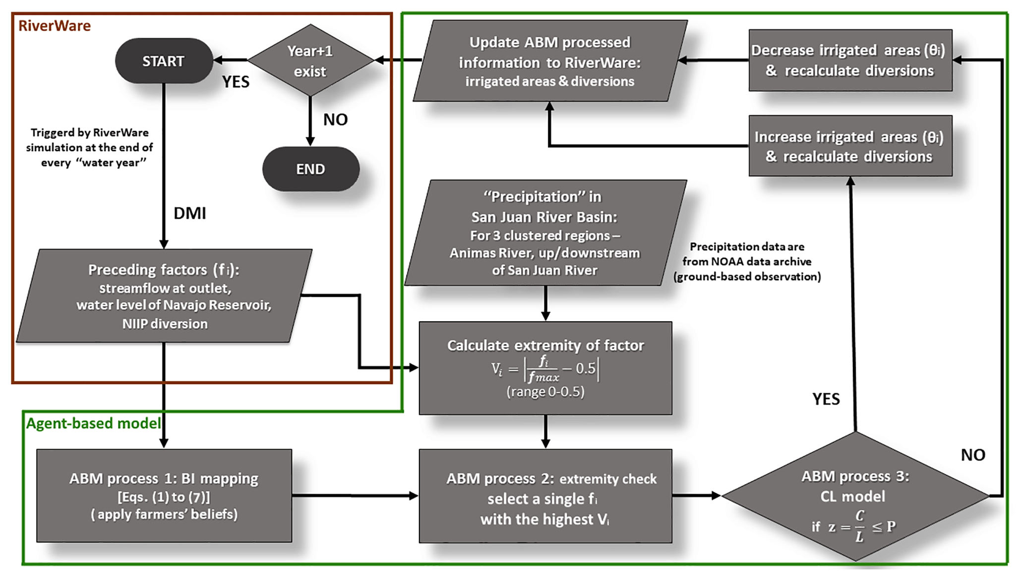
Figure 1The flow chart of agent decision-making process inside the two-way coupled ABM–RiverWare model (ABM.exe in Fig. S1). Agents make their decisions with uncertainty based on the method developed in this paper (joint BI mapping and CL model), and RiverWare runs the simulation based on these decisions.
3.1 Background of the study area
The San Juan River basin (Fig. 2) is the largest tributary of the Colorado River basin with a drainage area of 64 570 km2. Originating as snowmelt in the San Juan Mountains (part of the Rocky Mountains) of Colorado, the San Juan River flows 616 km through the deserts of northern New Mexico and southeastern Utah to join the Colorado River at Glen Canyon. Most water use activities are located in the upper part of the San Juan River basin in the states of New Mexico and Colorado. There are 16 major irrigation ditches, four cities, and two power plants (Fig. 2) located in this basin, for which the San Juan River is the primary water source. Major crops grown in the basin include hay, corn, and vegetables, and the main planting season runs from May to October (Census of Agriculture – San Juan County, New Mexico, 2012). The Navajo Reservoir, located 70 km upstream of the City of Farmington, NM, is the main water infrastructure in the basin (Fig. 2) which is used for flood control, irrigation, domestic and industrial water supply, and environmental flows. The reservoir is designed and operated by the US Bureau of Reclamation (USBR) following the rules in the Colorado River Storage Project (Annual Operating Plan for Colorado River Reservoirs, 2017). The active storage of the reservoir is 1.3 million acre-feet (1.6 billion cubic meters). The maximum release rate is limited to 5000 cubic feet per second (ft3 s−1) or 141.58 cubic meters per second (m3 s−1).

Figure 2The upper San Juan River basin. Different colors of the basin represent the geographical regions that this paper used to group major irrigation districts (agents, marked as dots). The location of the Navajo Reservoir is marked as a triangle.
The Navajo Indian Irrigation Project (NIIP) is another major water consumer within the basin beside the 16 major irrigation ditches. The NIIP supplies water to Native American tribes in the region. San Juan-Chama Project manages transbasin water transfers into the Rio Grande Basin, augmenting supply for Albuquerque, NM, irrigation and instream flow needs. Finally, the San Juan River Basin Recovery Implementation Program (SJRIP) implemented by the Fish and Wildlife Service manages environmental flows within the basin, dictating timing and magnitude of releases from the Navajo Reservoir and maintenance of a daily 500 ft3 s−1 (14.15 m3 s−1) minimum streamflow requirement (Behery, 2017).
To improve water planning and management in the basin, several state and federal agencies established a steering committee with the main responsibility of overseeing the institutional complexity for the water plans operated under the 1922 Colorado River Compact and 1948 Upper Colorado River Basin Compact. Although a regional water plan report (RWP) was updated in 2016 (State of New Mexico Interstate Stream Commission, 2016) by interested stakeholders, issues still exist under the terms of the 1948 Upper Colorado River Basin Compact. For example, New Mexico's entitled 642 380 ac-ft (0.793 billion cubic meters) consumptive use is substantially greater than the corresponding consumptive use.
The RWP summarizes the related information of water planning such as water rights, future water supply and demand projections, and newly available data. For example, 10 of the largest water users have cooperated to develop a shortage sharing agreement to keep the Navajo Reservoir from drawing down the reservoir pool elevation below 5990 ft (2041 m), which is the elevation required for NIIP diversion. The agreement stipulates that all parties share equally in shortages caused by drought (2013–2016 shortage agreement is available at https://www.fws.gov/southwest/sjrip/DR_SS03.cfm, last access: 2 May 2019). The RWP also projected that the total water demand in the basin is expected to increase due to the authorized expansion of the NIIP irrigation area, while a reduction of future water supply is possible due to climate change (State of New Mexico Interstate Stream Commission, 2016). Since irrigation activities are the most consumptive components of water demand among others (74.8 % of total water demand, State of New Mexico Interstate Stream Commission, 2016), collective adaptive actions of farmers will significantly affect the water planning and management in the San Juan Basin and become a suitable test bed for our methodology.
3.2 The BC-ABM–RiverWare model setup
USBR developed a RiverWare model for the San Juan River basin to support water management and resource planning efforts. RiverWare includes 19 irrigation ditch objects, 21 domestic and industrial use objects, 2 power plant objects, and 3 reservoir objects. Input data for the RiverWare model include historical tributary inflows, evapotranspiration rates for each irrigation ditch limited by the crop water requirement, historic water diversion for NIIP and the San Juan-Chama Project, and reservoir operation rules. Ungauged local inflows were determined by the simple closure of the local water budget. The model operates on a daily time step from 1 October 1928 to 30 September 2013 (85 years) with four cycles of simulation. Each cycle is a complete model run for the entire modeling period to fulfill part of the necessary information (e.g., some downstream water requirements need to be precalculated for the Navajo Reservoir to set up the release pattern). In this study, farmers that can make management decisions are quantified as 16 major irrigation ditch objects in RiverWare. They are defined as agents in the study and will decide whether to expand or reduce their irrigated area (e.g., management behavior, θ in Sect. 2) for the coming year at the end of every water year. We categorized the 16 agents into three groups based on their location (colored in Fig. 2). Agents in group 1 (light blue) were located upstream of the Navajo Reservoir, agents in group 2 (light green) were located on the Animas River (a major tributary of the San Juan River), and agents in group 3 (orange) were located downstream of the Navajo Reservoir.
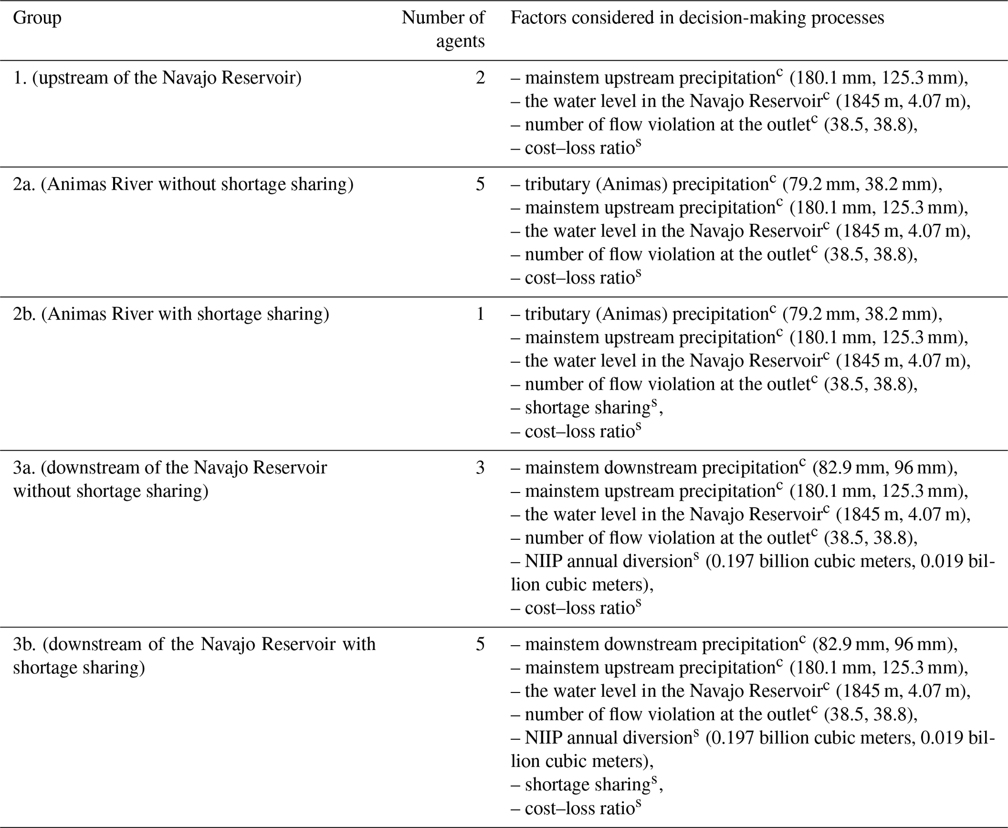
The BI mapping was applied to each group with different causal structures. The climatic preceding factors considered in this study include the mainstem (Navajo) upstream winter precipitation, the tributary (Animas River) winter precipitation, the mainstem downstream winter precipitation, the water level in the Navajo Reservoir, and the flow violations at the basin outlet (days below 500 ft3 s−1 or 14.15 m3 s−1 in a water year). The social preceding factors considered in this study include the cost–loss ratio, the NIIP diversions, and the shortage sharing. Table 1 summarizes the number of agents in each group and the proceeding factors they are considering. Given that agents are located at different places, the preceding factors that affect agents' decisions will also be different. This is an advantage of using ABM to incorporate spatial heterogeneity in the model.
Table 1Name of agent groups, number of agents in each group, and the proceeding factors considered in decision-making processes. Superscript “c” means climatic factors and superscript “s” means social factors. Numbers in the bracket are mean and standard deviation if applicable.
In this study, the information of winter precipitation was taken from NOAA ground-based rainfall monitoring gauges where we used the coming year's winter precipitation as a proxy for the snowpack forecast in the causal structure. Winter precipitation has a positive effect on snowpack but there is an uncertainty about how much snow will be accumulated. Therefore, when agents expect more winter precipitation, if they believe it will lead to a lot more snowpack, they will be more aggressive in the irrigated area expansion. Flow violation at the basin outlet and water level of the Navajo Reservoir are two system-wide preceding factors that are considered by all the three groups. When flow violation is too frequent or water level is too low, agents tend to be more conservative in the irrigated area expansion. If a shortage were declared, the RiverWare model would reduce the targeted streamflow at the basin outlet to 250 ft3 s−1 (7.08 m3 s−1) and the participating six agents would adjust their water diversion to achieve this newly targeted streamflow. Under the current model setting, agents follow the backward-looking, forward-acting mode, which means that agents make decisions based on their own past/current experiences (water level in the Navajo Reservoir, stream flow violations at the basin outlet, NIIP water diversion, and the previous decision on the irrigated area) and their belief of the winter precipitation forecast in the coming year. The detailed causal structure of BI mapping for each type of agent is given in the Supplement, where a standard Overview, Design concepts, and Details+Decision (ODD+D) protocol for ABM development is followed (Grimm et al., 2010).
To summarize, the data transfer from RiverWare to ABM at the end of a water year included (1) irrigation areas for the 16 irrigation agents, (2) the basin outflow, (3) water level in the Navajo Reservoir, and (4) the NIIP water diversion. After the completion of the ABM simulation, data transfer from ABM to RiverWare included (1) updated irrigated areas and (2) the corresponding water diversion of each agent. The next section will demonstrate the capability of the proposed model to recreate historical patterns in the San Juan Basin.
3.3 The BC-ABM–RiverWare model diagnostics
One of the major criticisms of ABM development is that ABM results are difficult to verify or validate (Parker et al., 2003; An et al., 2005, 2014; National Research Council, 2014). In this study, we address this concern by calibrating the coupled BC-ABM–RiverWare model to recreate the historical trend of (1) an individual agent's irrigated area and (2) San Juan River discharge. USBR provides the observed irrigated acreage for all 16 ditches and the flow measurements at two different locations along the San Juan River (at the outlet of the San Juan River basin and directly downstream of the Navajo Reservoir) for the calibration purpose. The calibrated parameters are the risk perception parameters (λ) and CL ratio (z) of each individual agent. Each agent has four λ's characterized by the relative geographical location with considered preceding factors. Unique values of λ are assigned to each preceding factor for each agent (through calibration) as different agents should have different levels of risk tolerance for different preceding factors. Different values of z are assigned to each agent representing the spatial heterogeneity of socioeconomic conditions. z is assumed to be constant for each agent throughout the model period as relative up-front cost information is unavailable. We also calibrate the irrigated areal increment of each agent to quantify the capability of different farmers for expanding or reducing their farmland. The actual irrigation area change at each year for each farmer is specified by the calibrated irrigated areal increment with an added uncertainty of 30 % representing the execution uncertainty of farmers. The thresholds of each preceding factor are also calibrated for calculating the extremities. A total of 102 parameters are manually calibrated (trial and error) with details explained in the Supplement (Supplement S2). In general, we calibrated the parameters sequentially from upstream and tributary agents (i.e., groups 1 and 2) to downstream (i.e., group 3). Within a group, we calibrated agents with the largest irrigated areas first to capture a better system-wide result.
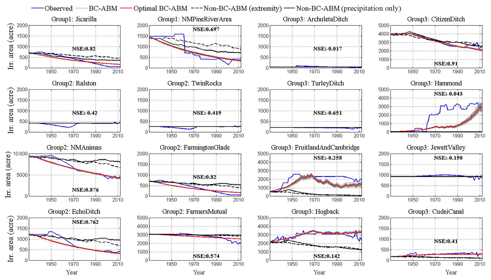
Figure 3The calibration results of the ABM–RiverWare model: individual agents' irrigated area changes from 1928 to 2013 organized by irrigation ditch and region (see groups in Fig. 3). Each figure includes the simulated irrigated area change from the best-fit BC-ABM (solid red) and the corresponding Nash–Sutcliffe efficiency (NSE), multiple runs of BC-ABM (solid gray) to visualize the stochasticity (30 runs) of agents' random behavior, non-BC-ABM with extremity (dashed black), and non-BC-ABM using precipitation only (solid black) against historical record (solid blue). 1 ac = 4046 m2.
The calibration results of irrigated areas are given in Fig. 3 and arranged by group (region). The blue curves are the historical irrigated area. The red curves are the best-fit result among multiple (30) modeling runs (shown by the gray curves, which represents the stochasticity) of each agent. In general, BC-ABM captures the pattern and trend of irrigated area for all agents, and we particularly focus on agents with the largest irrigated areas since their decision can dominate the basin. A figure showing the time variations of extremity values for each group of agents is given in the Supplement (see Fig. S2) to illustrate the preceding factors adopted by different groups of agents for making decisions at each time step.
The overall (area) weighted Nash–Sutcliffe efficiency (NSE, Nash and Sutcliffe, 1970) of the best-fit result is 0.55, which represents a reasonable calibration result. There are a few cases where structural changes occurred with some of the ditches that the model does not capture. Specifically, construction of the Navajo Reservoir in the 1960s inundated the New Mexico Pine River Ditch, while construction of the dam made it possible to expand the Hammond Irrigation Ditch (located directly downstream of the Navajo Reservoir). Similar structural changes are evident with the Echo, New Mexico, Animas, and Fruitland-Cambridge ditches. The model limitation associated with the use of BI mapping in ABM is discussed in the Discussion section.
To demonstrate the enhanced performance of the proposed BC-ABM framework in representing human decision-making processes, we conducted comparative experiments with conventional rule-based, deterministic ABMs (such as our previous work in Khan et al., 2017), referred to as the non-BC-ABMs. In the non-BC-ABMs, agents make decisions based on either past experience (e.g., flow violation or NIIP diversion) or future forecast (winter precipitation) alone, implying that agents have perfect foresight in terms of received information. Using precipitation as an example, an agent will expand irrigation area if the precipitation forecast is greater than the given threshold, and vice versa. Excluding BI mapping implies that the agents make decisions purely based on the forecast or new incoming information and fully ignore the information from past experience, while excluding the CL model means that the agents do not take socioeconomic factors into account when making decisions. Two non-BC-ABMs were tested and results are also shown in Fig. 3. The black solid curve represents the non-BC-ABM simulation still utilizing extremity for selecting the reference preceding factor, while the black dashed curve is the non-BC-ABM using only the precipitation in the decision-making processes. The better performance of the proposed BC-ABM framework, compared to the non-BC-ABMs, is evidenced by the closer agreements between the simulated and historical patterns of irrigated area from BC-ABM as well as weighted NSE (0.55 for BC-ABM vs. −1.25 for the non-BC-ABM with extremity and −1.39 for the non-BC-ABM with precipitation alone). Different non-BC-ABM simulations are also compared with the BC-ABM simulations as shown in Fig. S3.
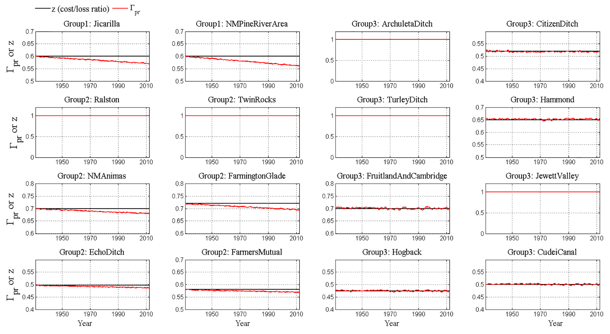
Figure 4Calibrated probability of expanding area (Γpr) and cost–loss ratio (z) for each agent.
The time variations of and calibrated z for each agent are shown in Fig. 4 to illustrate the characteristics of different agents, in terms of risk perception. The results show that the agents in group 1 and 2 have a consistently lower willingness to adjust irrigation area (Γpr shown in red) compared to the corresponding CL ratio (z shown in black). In contrast, group-3 agents adjust irrigation area more often as evidenced by the frequent crossover between red and black curves, which suggest that agents in group 3 are relatively risk-neutral compared to those in group 1 and 2. The calibration results of basin outflow and the Navajo Reservoir inflow are given in Fig. 5. The results show that the simulated values agree closely with the historical observations evidenced by the NSEs of 0.60 and 0.54, respectively. We do notice that our coupled BC-ABM–RiverWare model misses peaks of streamflow possibly due to the lower input streamflow data of RiverWare. However, since our focus is the water-scarce situation in this case study, this underestimation does not significantly affect our following analysis.
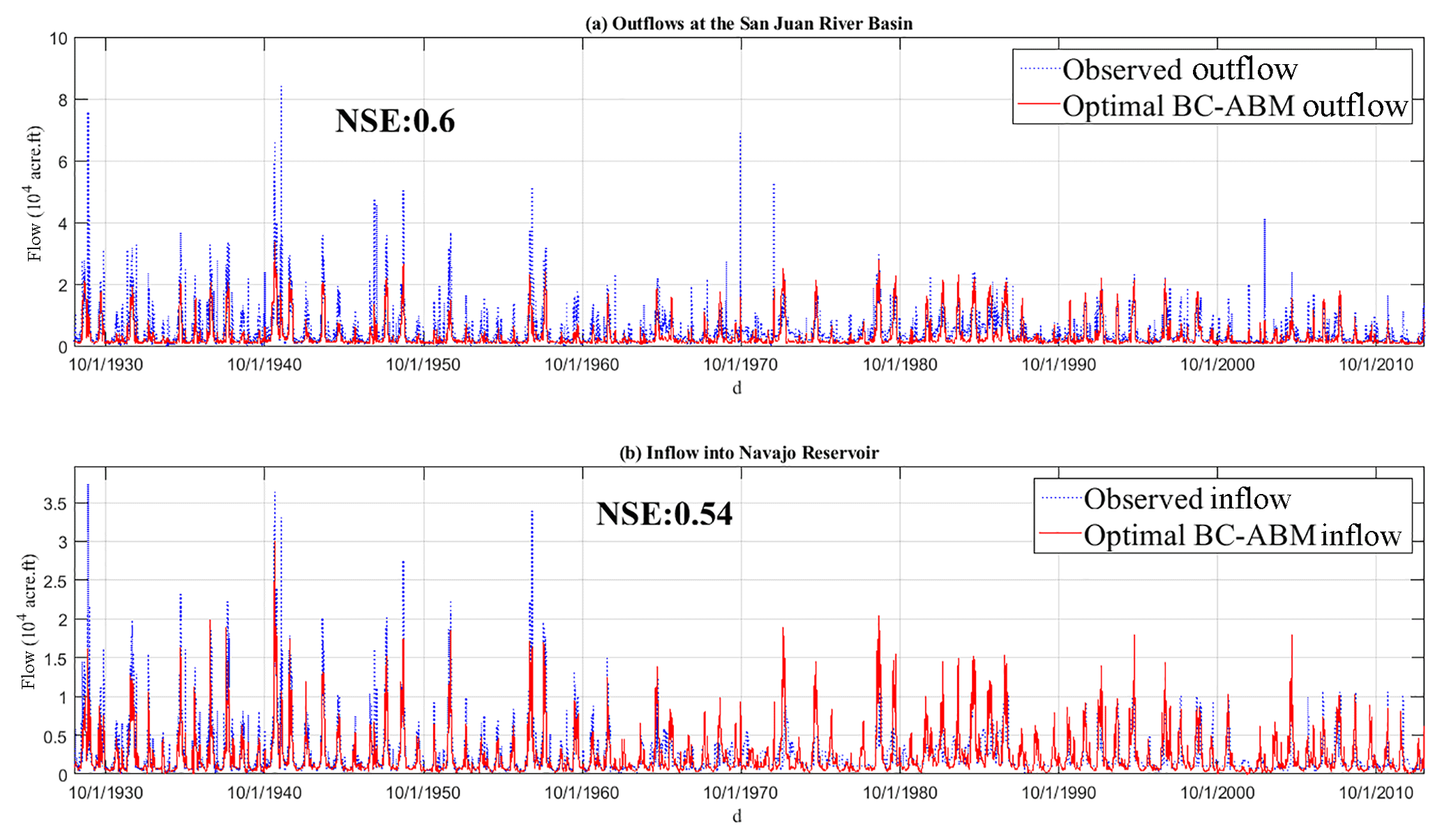
Figure 5The calibration results of the ABM–RiverWare model: (a) the basin outflow to the Colorado River; (b) inflow to the Navajo Reservoir. Blue lines are historical data and red lines are modeling results. 1 ac-ft = 1234 m3.
The calibration results in Sect. 3.3 demonstrate the credibility of the coupled BC-ABM–RiverWare model in representing human psychological, uncertain decision-making processes. The encouraging results suggest that we can apply the proposed BC-ABM framework to test some extreme conditions to perform different scenario analyses. Two scenarios are tested in this section: the effect of changing agents' risk perception and the effect of changing socioeconomic condition.
4.1 The effect of changing agents' risk perception
Different risk perception scenarios are tested by making a stepwise change in all agents' λ values from 0.5 (risk-averse) to 1 (risk-seeking). The basin-wide results are summarized in Fig. 6, which shows the key measure quantities including the cumulative probability distribution of annual total irrigated area, the Navajo Reservoir water level in December, annual total downstream flow violation frequency, and volume. The simulations under extreme risk-averse (λ=0.5) and risk-seeking (λ=1) scenarios are shown in blue and green, while those with calibrated historical risk perceptions for each agent are shown in red, referred to as the baseline. The gray curves lying between blue and green are the results corresponding to different λ values. The total irrigation area generally increases with an increasing λ, indicating that the agents become more risk-seeking if they are more confident about new incoming information.

Figure 6The cumulative density frequency throughout the entire simulation period of (a) the basin-wide irrigated area, (b) the Navajo Reservoir end-of-year water level, (c) basin outlet annual streamflow violation days, and (d) basin outlet annual streamflow violation volume. Results are given for the calibrated (green curves), risk-averse (blue curves), and risk-seeking (red curves) cases. The simulation results with different values of agents' risk perceptions (λ) between 0.5 and 1 are shown in gray.
There are two interesting observations. First, it is clear that when all agents become risk-seeking, their emerging actions will result in a larger irrigated area in the basin (Fig. 6a). Since all agents want to expand their irrigated area, the Navajo Reservoir will reserve more water at the end of each year, resulting in slightly higher water levels (Fig. 6b). Streamflow violations show a somewhat counterintuitive result. The volume of violation under risk-seeking scenarios increases as expected (green curve shifts to right in Fig. 6d), but the frequency of violation decreases (green curve shifts to left in Fig. 6c). This is due to the fact that the Navajo Reservoir holds more water for irrigation season to satisfy downstream increasing water demand, which results in much fewer streamflow violation days during the irrigation season. Although this operation slightly increases streamflow violation days in the following season, the total number of violation days still decreases (Fig. S4). Second, the baseline results (red curves) are closer to the “all agents risk-averse” scenario results (blue curves). This is consistent with the findings from previous studies (e.g., Tena and Gómez, 2008), which suggest that farmers are commonly risk-averse when the stakes are high (Matte et al., 2017).

Figure 7Individual agents' irrigated area changes under calibrated (green curves), risk-averse (blue curves), and risk-seeking (red curves) scenarios. The simulation results with different values of agents' risk perceptions (λ) between 0.5 and 1 are shown in gray. 1 ac = 4046 m2.
We also look at the time variations of individual irrigated area changes for characterizing risk perceptions of different agents. Figure 7 shows the simulated irrigation area changes for four selected large irrigation ditched since they are the major players in the basin. The results clearly show that Jicarilla (group 1) and NMAnimas (group 2) are historically risk-averse agents (red curves overlap with blue curves). In contrast, Hammond and Hogback (group 3) are relatively risk-neutral, compared to agents in group 1 and 2, as the red curves lie in between the green and blue curves. Group-3 agents are located downstream of the Navajo Reservoir and most of them consider the Navajo Reservoir as a steady water source, so they can have relatively more aggressive attitudes toward risk compared to their upstream counterparts. Also, note that Jicarilla, Hammond, and Hogback under the risk-seeking scenario eventually reach their maximum available irrigated area. Therefore, their irrigated area flattens out at the end of the simulation. The gray curves in Fig. 7 represent the simulated irrigation area changes for agents corresponding to different agents' risk perceptions. It shows that the irrigation area generally increases with an increasing λ for all the four agents.
4.2 The effect of changing socioeconomic condition
The proposed BC-ABM framework allows us to quantify the influences of external socioeconomic factors on human decision-making processes by adjusting the CL ratio. In this study, we conducted a sensitivity analysis on the cost–loss ratio to test what happens if economic conditions change and it becomes more expensive or cheaper to expand the irrigated area by systematically increasing (+10 % and +20 %) or decreasing (−10 % and −20 %) z values for all agents. When the z value goes up, it means that the cost of increasing irrigated area goes up, or the opportunity loss of not increasing irrigated area goes down. In either case, the situation should become harder for agents to expand their irrigated area. When the z value goes down, following the same logic, the economic conditions become easier for agents to expand their irrigated area. The modeling results shown in Fig. 8 fit with this intuition quite well. All blue and cyan curves (increasing z values) are located below, and purple and magenta curves (decreasing z values) are located above red curves (baseline). Modeling results also show that, in the basin, groups 1 and 2 are less sensitive to the changes in economic conditions but agents in group 3 are more sensitive to the economic conditions. Of course, individual differences exist inside each group.
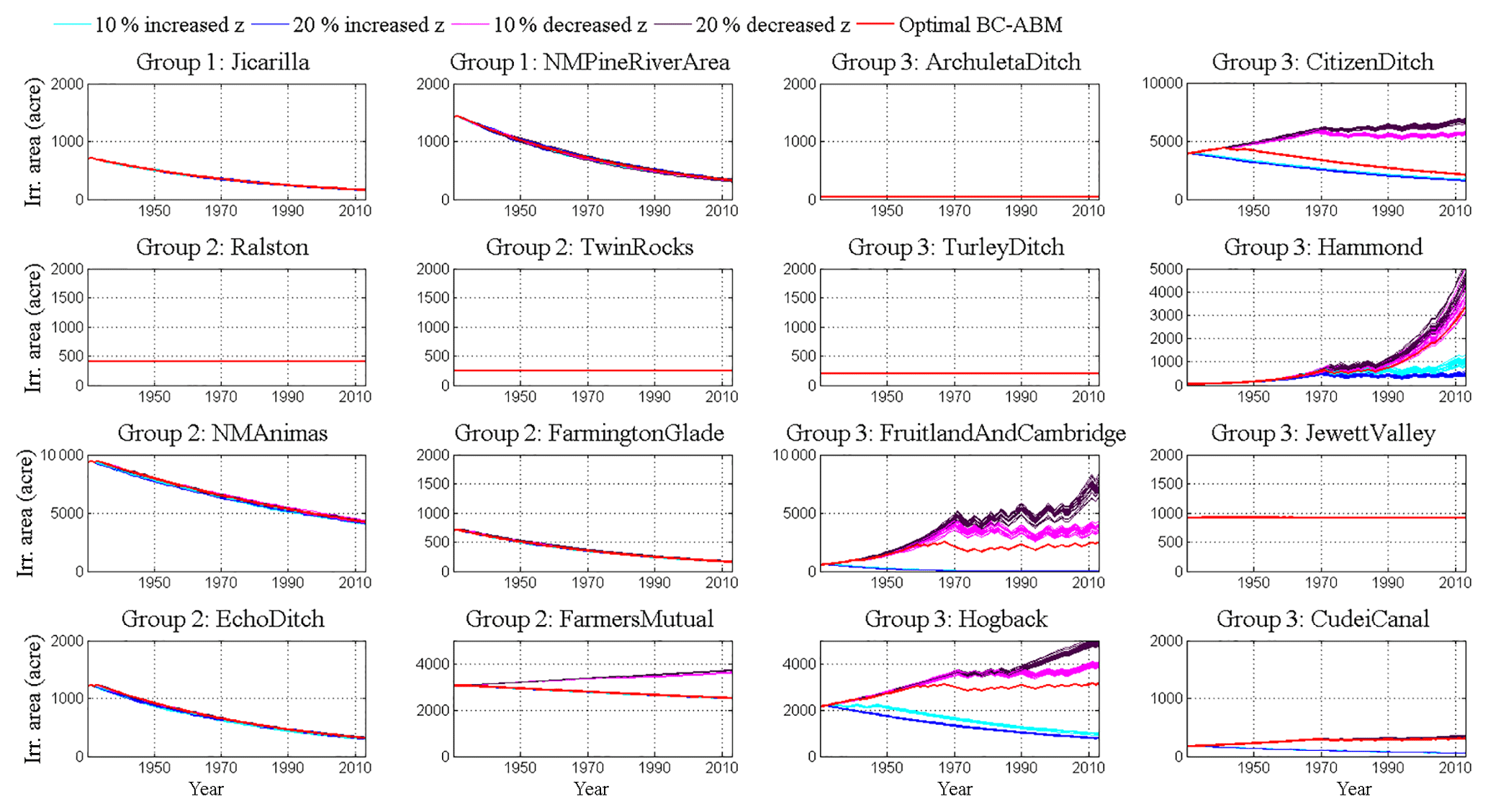
Figure 8The sensitivity analysis of changing economic conditions on an agent's decision on irrigated areas. Blue (+20 %) and cyan (+10 %) curves represent increasing z values which make area expansion more expensive. Purple (−20 %) and magenta (−10 %) lines represent decreasing z values which make area expansion cheaper. 1 ac = 4046 m2.
According to the San Juan River basin regional water plan, several strategies and constructions such as on-farm and canal improvements and the municipal and irrigation pipeline from the Navajo Reservoir will be authorized for meeting the future water demand (State of New Mexico Interstate Stream Commission, 2016). These strategies and constructions could lead to a change in future socioeconomic conditions, in terms of the cost of water usage and changing irrigated area (e.g., up-front cost) for stakeholders. In this study, we quantify the effects of up-front cost on the changes of irrigation area (i.e., irrigation water demand) using the proposed BC-ABM framework. We can look at the influence of up-front cost on human decision-making processes from two perspectives. First, it directly changes the socioeconomic condition of an agent (change of CL ratio). Second, it influences an agent's decision-making processes by introducing more information (change of causal network in BI mapping). As a result, the proposed BC-ABM framework can take up-front costs into account without theoretical and technical difficulties if related information is available. Two scenarios assuming a general increasing and decreasing up-front cost for agents over time are tested in the study. For each agent, a time varied z is generated by adding a positive/negative trend with a small random fluctuation to the calibrated z to mimic the spatial and temporal heterogeneity of up-front costs. Note that we did not include up-front costs into the current BI mapping as real-world stakeholders' inputs are needed to recalibrate all the model parameters.
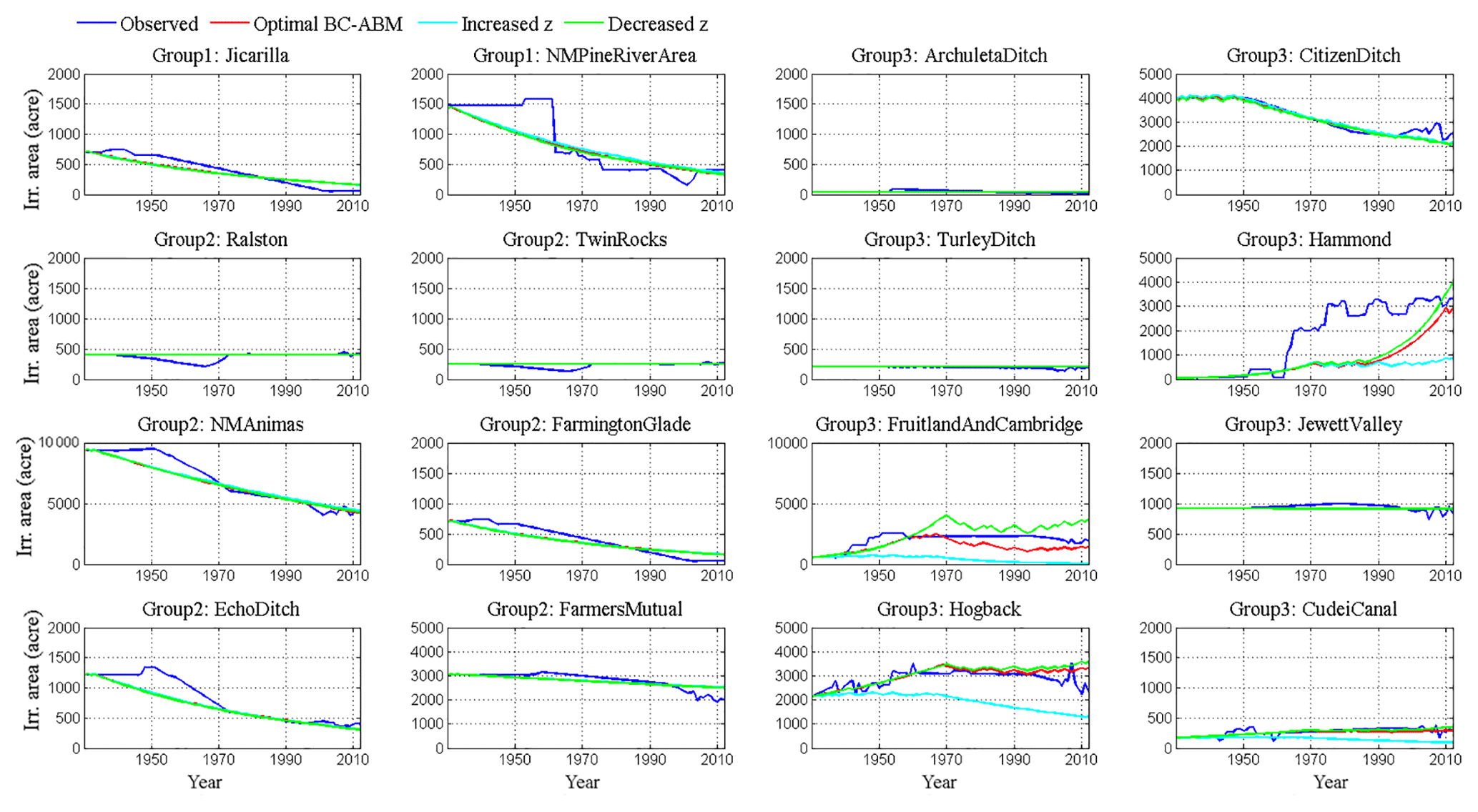
Figure 9Irrigation area changes of each agent under the scenario of increasing (cyan) and decreasing (green) z. The calibrated results (baseline simulation) are shown in red and observations are shown in blue. 1 ac = 4046 m2.
The time variation of irrigated area for all 16 agents under different up-front cost trends is shown in Fig. 9. The cyan and green curves are the irrigated area change under an increasing and decreasing z, respectively, while red curves are the baseline which uses calibrated z values. The results show that the influence of changing z on group-3 agents is relatively significant compared to group 1 and group 2. A consistently higher (lower) green (cyan) curve as compared to the baseline is observed. These preliminary results are expected as they fit the economic intuition. In this specific case, farmers tend to expand their irrigation area earlier (by comparing cyan and red curves) if they expect a corresponding increased cost in the future. In contrast, if the cost of expanding irrigation area in the future is expected to go down, farmers will defer the actions to pursue a lower cost.
5.1 Generalized modeling framework and policy implementation for other basins
The proposed BC-ABM framework in this paper is intended to be a generalizable approach in water resources management and other fields that need to quantify human decisions. This framework directly addresses the four challenges summarized by Scalco et al. (2018) about how to apply the TPB in an agent-based setting. The model diagnostic process and the use of the historical irrigated area answer the first challenge: data and preliminary model assessment. Applying the BI mapping provides a stochastic representation of the decision-making process which eliminates the concern of working with a static model. Combing with the CL model, we can mathematically calculate when does intention become behavior. Finally, coupling the ABM with RiverWare is our solution to address the feedback mechanisms challenge in a CNHS. The method can be applied to other basins given that the required input data for BI mapping are publically available, such as the precipitation from NOAA and the streamflow from USGS, and risk perception (λ) and CL ratio (z) are calibrated parameters. However, the data required for the model diagnostic and calibration, such as long-term historical irrigated area time series, might not be available in every basin. In this situation, if one intends to duplicate the proposed method in other basins, some alternative data source, such as land use and land cover change data from USGS, can be used as a proxy of calibration targets.
The modeling results can be used to inform water management policy. For example, the sensitivity analysis (see Fig. 8) suggests that the collective action of farmers has the potential to influence the irrigation of 4.5×10⁴ to 6.1×10⁴ ac (182.1 to 246.9 km2) of cropland with 9000 to 12 000 ac-ft (11.1 to 14.8 million cubic meters) of water demand, which is about 30 % to 39 % of the average annual water usage under changing economic conditions (i.e., 20 % increase or decrease in up-front cost). A potential increase/decrease in future irrigation cost could also influence farmers' decisions. Understanding such behavior is also critical to future water resource planning and management in the San Juan River basin as (1) threat of climate change will lead to a shift in timing of flows associated with a mean decrease in future water supply resulting from an anticipated reduced precipitation and/or increased evaporation, and (2) there are several settlement agreements with the tribal communities along the San Juan River basin where their committed allotment of water has yet to be put to full use (e.g., Navajo-Gallup pipeline and Navajo Indian Irrigation Project that both require construction and/or expansion of existing water delivery infrastructure to make full use of water rights).
5.2 Model limitations
Here we discuss two areas of limitation of the current study: data availability and model structure. The lack of historical data to serve as the calibration target is mentioned in the above section. Another data limitation is the CL ratio calculation and the up-front cost. Currently, the CL ratio is treated as a calibrated parameter in BC-ABM framework. The value of the CL ratio can be estimated directly by acquiring relevant data, if available. For example, the farm production expense data provided by the US Department of Agriculture could be used as an approximation of the expected cost of changing irrigation area (C in Eq. 10), while the farm income and wealth statistics estimated from crop production may be considered as a major part of opportunity loss (L in Eq. 10). The third data limitation is the necessary data to create the precise causal structure of BI mapping (Cheng et al., 2002; Premchaiswadi et al., 2010). In general, an accurate causal structure of BI mapping can be obtained by detailed interviews with decision makers (O'Keeffe et al., 2016) or learned from a dataset (Sutheebanjard and Premchaiswadi, 2010).
Regarding the model structure limitation, the farmer's belief is currently calculated using one single preceding factor in the cognitive map that has the most extremity. The use of extremity from a single preceding factor in the decision-making processes assumes that the joint probability of decision-making from multiple preceding factors is not taken into account (the agent may not respond to the cumulative effects of environmental conditions). Finally, the current method does not explicitly consider direct interaction among agents in the BI mapping. We do model agents as interacting indirectly through irrigated water withdrawal (i.e., upstream agents' water uses will affect downstream agents' water availability). However, effects like peer pressure, word of mouth, and potential water markets are not currently considered in the model.
Making water resources management decisions in a complex adaptive natural–human system subject to uncertain information is a challenging issue. The interaction between human and natural systems needs to be modeled explicitly with associated uncertainties quantified and managed in a formal manner. This study applies a two-way coupled agent-based model (ABM) with a river-reservoir management model (RiverWare) to address the interaction between human and natural systems. The proposed ABM framework characterizes human decision-making processes by adopting a perspective of the theory of planned behavior implemented using Bayesian inference (BI) mapping joined with cost–loss (CL). The advantage of ABM is that, by defining different agents, various human activities can be represented explicitly while the coupled water system provides a solid basis to simulate the feedback between the environment and agents.
Combining BI mapping and CL modeling allows us to (1) explicitly describe human decision-making processes, (2) quantify the associated decision uncertainty caused by incomplete/ambiguous information, and (3) examine the adaptive water management in response to a changing natural environment as well as socioeconomic conditions. Calibration results for this coupled BC-ABM–RiverWare model, as demonstrated in the San Juan River basin, show that this methodology can capture the historical pattern of both human activities (irrigated area changes) and natural dynamics (streamflow changes) while quantifying the risk perception of each agent via risk perception parameters (λ). The scenario results also show that the majority of agents in the basin are risk-averse, which confirms the conclusion of Tena and Gómez (2008). The improved representation of the proposed BC-ABM is evidenced by the closer agreement of BC-ABM simulations against observations, compared to those from an ABM without using BI mapping and CL ratio. Changing economic conditions also yield intuitive agent behavior; that is, when crop area expansion is more expensive/cheaper, fewer/more agents will do it.
Future work can target further methodology development to include direct agent interaction into the BI mapping. For example, agents' decisions can be affected by observing their neighbors' actions, and this information will always be treated with λ=1. This means agents will always believe their own observations (i.e., to see is to believe). In addition, we only defined groups of farmers as agents in this study. Future work can seek to add power plants, cities/municipalities, and reservoirs as agents. The direct and indirect interaction among these different types of agents (such as farmers and power plants, who may or may not have to compete for water from the reservoir) will provide a more comprehensive picture in the entire food–energy–water–environment nexus.
The input data and modeling results of the ABM-RiverWare model are available at https://dx.doi.org/10.25584/data.2019-05.722/1510802 (Hyun et al., 2019).
The supplement related to this article is available online at: https://doi.org/10.5194/hess-23-2261-2019-supplement.
YCEY led the entire project. JYH, SYH, and YCEY developed the ABM. VT prepared RiverWare. JM reviewed the model coupling. SYH and YCEY prepared the manuscript with contributions from all co-authors.
The authors declare that they have no conflict of interest.
This research was supported by the Office of Science of the US Department of Energy as part of research in the Multi-Sector Dynamics, Earth and Environmental System Modeling Program. We want to thank the editor and anonymous reviewers, who helped us improve the quality of this paper. Special thanks are given to Susan Behery in USBR for providing historical data on the San Juan Basin and Majid Shafiee-Jood in the University of Illinois, who discussed the methods of BI mapping and CL modeling with us in the earlier version of the manuscript. All data used for both the RiverWare model (inflow, crop ET, and water diversion, etc.) and the agent-based model (winter precipitation, historical basin outflow, and historical irrigated area, etc.) are explicitly cited in the reference list.
This paper was edited by Pieter van der Zaag and reviewed by Andres Baeza and one anonymous referee.
Ajzen, I.: The theory of planned behavior, Organ. Behav. Hum. Decis. Process., 50, 179–211, https://doi.org/10.1016/0749-5978(91)90020-T, 1991.
An, L., Linderman, M., Qi, J., Shortridge, A., and Liu, J.: Exploring complexity in a human environment system: an agent-based spatial model for multidisciplinary and multi-scale Integration, Ann. Assoc. Am. Geogr., 95, 54–79, https://doi.org/10.1111/j.1467-8306.2005.00450.x, 2005.
An, L., Zvoleff, A., Liu, J., and Axinn, W.: Agent-based modeling in coupled human and natural systems (CHANS): Lessons from a comparative analysis, Ann. Assoc. Am. Geogr, 104, 723–745, https://doi.org/10.1080/00045608.2014.910085, 2014.
Annual Operating Plan for Colorado River Reservoirs: US Department of the Interior Bureau of Reclamation, available at: https://www.usbr.gov/uc/water/rsvrs/ops/aop/ (last access: 7 May 2019), 2017.
Baggett, S., Jeffrey, P., and Jefferson, B.: Risk perception in participatory planning for water reuse, Desalination, 187, 149–158, https://doi.org/10.1016/j.desal.2005.04.075, 2006.
Behery, S.: Current status of Navajo Reservoir, available at: https://www.usbr.gov/uc/water/crsp/cs/nvd.html (last access: 7 May 2019), 2017.
Berglund, E. Z.: Using agent-based modeling for water resources planning and management, J. Water Res. Plan. Man., 141, 04015025, https://doi.org/10.1061/(ASCE)WR.1943-5452.0000544, 2015.
Brown, C. M., Ghile, Y., Laverty, M., and Li, K.: Decision scaling: Linking bottom-up vulnerability analysis with climate projections in the water sector, Water Resour. Res., 48, W09537, https://doi.org/10.1029/2011WR011212, 2012.
Brown, C. M., Lund, J. R., Cai, X., Reed, P. M., Zagona, E. A., Ostfeld, A., Hall, J., Characklis, G. W., Yu, W., and Brekke, L.: The future of water resources systems analysis: toward a scientific framework for sustainable water management, Water Resour. Res., 51, 6110–6124, https://doi.org/10.1002/2015WR017114, 2015.
Census of Agriculture (county profile) – San Juan County, New Mexico: National Agricultural Statistics Service, US Department of Agriculture, New Mexico Field Office, Las Cruces, NM, USA, 70 pp., 2012.
Cheng, J., Greiner, R., Kelly, J., Bell, D., and Liu, W.: Learning Bayesian Networks from Data: An Information-Theory Based Approach, Artif. Intell., 137, 43–90, https://doi.org/10.1016/S0004-3702(02)00191-1, 2002.
Denaro, S., Castelletti, A., Giuliani, M., and Characklis, G. W.: Fostering cooperation in power asymmetrical water systems by the use of direct release rules and index-based insurance schemes, Adv. Water Resour., 115, 301–314, https://doi.org/10.1016/j.advwatres.2017.09.021, 2017.
Di Baldassarre, G., Viglione, A., Carr, G., Kuil, L., Yan, L., Brandimarte, K., and Blöschl, G.: Debates–Perspectives on socio-hydrology: Capturing feedbacks between physical and social processes, Water Resour. Res., 51, 4770–4781, https://doi.org/10.1002/2014WR016416, 2015.
Dorazio, R. M. and Johnson, F. A.: Bayesian inference and decision theory – a framework for decision making in natural resource management, Ecol. Appl., 13, 556–563, 2003.
Draper, A. J., Munévar, A., Arora, S., Reyes, E., Parker, N., Chung, F., and Peterson, L.: CalSim: A generalized model for reservoir system analysis, J. Water Res. Plan. Man., 130, 480–489, https://doi.org/10.1061/(ASCE)0733-9496(2004)130:6(480), 2004.
Giuliani, M. and Castelletti, A.: Assessing the value of cooperation and information exchange in large water resources systems by agent-based optimization, Water Resour. Res., 49, 3912–3926, https://doi.org/10.1002/wrcr.20287, 2013.
Giuliani, M., Castelletti, A., Amigoni, F., and Cai, X.: Multiagent systems and distributed constraint reasoning for regulatory mechanism design in water management, Water Res. Plan. Man., 141, 04014068, https://doi.org/10.1061/(ASCE)WR.1943-5452.0000463, 2015.
Giuliani, M., Li, Y., Castelletti, A., and Gandolfi, C.: A coupled human-natural systems analysis of irrigated agriculture under changing climate, Water Resour. Res., 52, 6928–6947, https://doi.org/10.1002/2016WR019363, 2016.
Grimm, V., Berger, U., DeAngelis, D. L., Polhill, J. G., Giske, J., and Railsback, S. F.: The ODD protocol: A review and first update, Ecol. Model., 221, 2760–2768, https://doi.org/10.1016/j.ecolmodel.2010.08.019, 2010.
Groeneveld, J., Müller, B., Buchmann, C., Dressler, G., Guo, C., Hase, N., Homann, F., John, F., Klassert, C., Lauf, T., Liebelt, V., Nolzen, H., Pannicke, N., Schulze, J., and Weise, H.: Theoretical foundations of human decision-making in agent-based land use models – A review, Environ. Model. Softw., 87, 39–48, https://doi.org/10.1016/j.envsoft.2016.10.008, 2017.
Hameed, T. and O'Neill, R.: River Management Decision Modeling in IQQM, Melbourne, Australia, available at: https://www.mssanz.org.au/modsim05/papers/hameed.pd (last access: 7 May 2019), 2005.
Hu, Y., Quinn, C. J., Cai, X., and Garfinkle, N. W.: Combining human and machine intelligence to derive agents' behavioral rules for groundwater irrigation, Adv. Water Resour., 109, 29–40, https://doi.org/10.1016/j.advwatres.2017.08.009, 2017.
Hyun, J. Y., Huang, S. Y., Yang, Y. C. E., Tidwell, V., and Macknick J.: San Juan ABM-RiverWare Input and Result Data, IM3 Data Repository, https://doi.org/10.25584/data.2019-05.722/1510802, last access: 8 May 2019.
Johnson, J.: MODSIM versus RiverWare: A comparative analysis of two river reservoir modeling tools, Report 2014.3669, US Department of the Interior-Bureau of Reclamation, Pacific Northwest Region, Boise, Idaho, 2014.
Keeney, R. L.: Decision analysis: an overview, Oper. Res., 30, 803–838, https://doi.org/10.1287/opre.30.5.803, 1982.
Khan, H. F., Yang, Y. C. E., Xie, H., and Ringer, C.: A coupled modeling framework for sustainable watershed management in transboundary river basins, Hydrol. Earth Syst. Sci., 21, 6275–6288, https://doi.org/10.5194/hess-21-6275-2017, 2017.
Knight, F. H.: Risk, Uncertainty, and Profit. Houghton Miffin, New York, 1921.
Kocabas, V. and Dragicevic, S.: Bayesian networks and agent-based modeling approach for urban land-use and population density change: A BNAS model, J. Geogr. Syst., 36, 1–24, https://doi.org/10.1007/s10109-012-0171-2, 2012.
Lee, K.-K. and Lee, J.-W.: The economic value of weather forecasts for decision-making problems in the profit/loss situation, Met. Apps., 14, 455–463, https://doi.org/10.1002/met.44, 2007.
Li, Y., Giuliani, M., and Castelletti, A.: A coupled human–natural system to assess the operational value of weather and climate services for agriculture, Hydrol. Earth Syst. Sci., 21, 4693–4709, https://doi.org/10.5194/hess-21-4693-2017, 2017.
Liu, J., Dietz, T., Carpenter, S. R., Alberti, M., Folke, C., Moran, E., Pell, A. N., Deadman, P., Kratz, T., Lubchenco, J., Ostrom, E., Ouyang, Z., Provencher, W., Redman, C. L., Schneider, S. H., and Taylor, W. W.: Complexity of coupled human and natural systems, Science, 317, 1513–1516, https://doi.org/10.1126/science.1144004, 2007.
Manson, S. M. and Evans, T.: Agent-based modeling of deforestation in southern Yucatán, Mexico, and reforestation in the Midwest United States, P. Natl. Acad. Sci. USA, 104, 20678–20683, https://doi.org/10.1073/pnas.0705802104, 2007.
Matte, S., Boucher, M.-A., Boucher, V., and Filion, T.-C. F.: Moving beyond the cost-loss ratio: economic assessment of streamflow forecasts for a risk-averse decision maker, Hydrol. Earth Syst. Sci., 21, 2967–2986, https://doi.org/10.5194/hess-21-2967-2017, 2017.
Müller, B., Bohn, F., Dreßler, G., Groeneveld, J., Klassert, C., Martin, R., Schlüter, M., Schulze, J., Weise, H., and Schwarz, N.: Describing human decisions in agent-based models – ODD+D, an extension of the ODD protocol, Environ. Model. Softw., 48, 37–48, https://doi.org/10.1016/j.envsoft.2013.06.003, 2013.
Mulligan, K., Brown, C. M., Yang, Y. C. E., and Ahlfeld, D.: Assessing groundwater policy with coupled economic-groundwater hydrologic modeling, Water Resour. Res., 50, 2257–2275, https://doi.org/10.1002/2013WR013666, 2014.
Murphy, A. H.: Decision-making models in the cost-loss ratio situation and measures of the value of probability forecasts, Mon. Weather Rev., 104, 1058–1065, https://doi.org/10.1175/1520-0493(1976)104<1058:DMMITC>2.0.CO;2, 1976.
Murphy, A. H., Katz, R. W., Winkler, R. L., and Hsu, W.-R.: Repetitive decision making and the value of forecasts in the cost-loss ratio situation: a dynamic model, Mon. Weather Rev., 113, 801–813, https://doi.org/10.1175/1520-0493(1985)113<0801:RDMATV>2.0.CO;2, 1985.
Nash, J. E. and Sutcliffe, J. V.: River flow forecasting through conceptual models part I – A discussion of principles, J. Hydrol., 10, 282–290, 1970.
National Research Council: Advancing Land Change Modeling: Opportunities and Research Requirements, National Academies Press, Washington, DC, 2014.
Ng, T. L., Eheart, J. W., Cai, X., and Braden, J. B.: An agent-based model of farmer decision making and water quality impacts at the watershed scale under markets for carbon allowances and a second-generation biofuel crop, Water Resour. Res., 47, W09519, https://doi.org/10.1029/2011WR010399, 2011.
O'Keeffe, J., Buytaert, W., Mijic, A., Brozović, N., and Sinha, R.: The use of semi-structured interviews for the characterization of farmer irrigation practices, Hydrol. Earth Syst. Sci., 20, 1911–1924, https://doi.org/10.5194/hess-20-1911-2016, 2016.
Pahl-Wostl, C., Távara, D., Bouwen, R., Craps, M., Dewulf, A., Mostert, E., Ridder, D., and Taillieu, T.: The importance of social learning and culture for sustainable water management, Ecol. Econ., 64, 484–495, https://doi.org/10.1016/j.ecolecon.2007.08.007, 2008.
Parker, D. C., Manson, S. M., Janssen, M. A., Hoffmann, M. J., and Deadman, P.: Multi agent systems for the simulation of land-use and land-cover change: A review, Ann. Assoc. Am. Geogr., 93, 314–337, https://doi.org/10.1111/1467-8306.9302004, 2003.
Pope, A. J. and Gimblett, R.: Linking Bayesian and agent-based models to simulate complex social-ecological systems in semi-arid regions, Front. Environ. Sci., 3, https://doi.org/10.3389/fenvs.2015.00055, 2015.
Premchaiswadi, W., Jongsawat, N., and Romsaiyud, W.: Bayesian Network Inference with Qualitative Expert Knowledge for Group Decision Making. In: 5th IEEE International Conference on Intelligent Systems (IS), IEEE Press, New York, 126–131, 2010.
RiverWare Technical Documentation – Data Management Interface: Center for Advanced Decision Support for Water and Environmental Systems, University of Colorado, Boulder, CO, 2017.
Scalco, A., Ceschi, A., and Sartori, R.: Application of Psychological Theories in Agent-Based Modeling: The Case of the Theory of Planned Behavior, Nonlin. Dynam. Psychol., 22, 15–33, 2018
Schlüter, M., Leslie, H., and Levin, S.: Managing water-use trade-offs in a semi-arid river delta to sustain multiple ecosystem services: a modeling approach, Ecol. Res., 24, 491–503, https://doi.org/10.1007/s11284-008-0576-z, 2009.
Schlüter, M., Baeza, A., Dressler, G., Frank, K., Groeneveld, J., Jager, W., Janssen, M. A., McAllister, R. R. J., Müller, B., Orach, K., Schwarz, N., and Wijermans, N.: A framework for mapping and comparing behavioural theories in models of social-ecological systems, Ecol. Econ., 131, 21–35, https://doi.org/10.1016/j.ecolecon.2016.08.008, 2017.
Sedki, K. and de Beaufort, L. B.: Cognitive maps for knowledge representation and reasoning, Tools with Artificial Intelligence (ICTAI), in: 24th International Conference, Athens, Greece, November 2012, 1035–1040, https://doi.org/10.1109/ICTAI.2012.175, 2012.
Shafiee-Jood, M., Cai, X., and Deryugina, T.: A theoretical method to investigate the role of farmers' behavior in adopting climate forecasts, World Environmental and Water Resources Congress 2017 – Creative Solution for a Changing Environment, Sacramento, CA, 2017.
Sharma, L. K., Kohl, K., Margan, T. A., and Clark, L. A.: Impulsivity: relations between self-report and behavior, J. Pers. Soc. Psychol., 104, 559–575, https://doi.org/10.1037/a0031181, 2013.
State of New Mexico Interstate Stream Commission: San Juan Basin Regional Water Plan, available at: http://www.ose.state.nm.us/Planning/RWP/region_02.php (last access: 7 May 2019), 2016.
Sutheebanjard, P. and Premchaiswadi, W.: Analysis of calendar effects: Day-of-the-week effect on the stock exchange of Thailand (SET). International Journal of Trade, Int. P. Econ. Dev. Res., 1, 57–62, https://doi.org/10.7763/IJTEF.2010.V1.11, 2010.
Tena, E. C. and Gómez, S. Q.: Cost-Loss decision models with Risk Aversion, Working paper 01/08, Universidad Complutense de Madrid, 2008.
Thompson, J. C.: On the operational deficiencies in categorical weather forecasts, B. Am. Meleorol. Soc., 33, 223–226, 1952.
Troy, T. J., Pavao-Zuckerman, M., and Evans, T. P.: Debates n– Perspectives on socio-hydrology: Socio-hydrologic modeling: Tradeoffs, hypothesis testing, and validation, Water Resour. Res., 51, 4806–4814, https://doi.org/10.1002/2015WR017046, 2015.
Yang, Y. C. E., Cai, X., and Stipanović, D. M.: A decentralized optimization algorithm for multi-agent system based watershed management, Water Resour. Res., 45, W08430, https://doi.org/10.1029/2008WR007634, 2009.
Yang, Y. C. E., Zhao, J., and Cai, X.: A decentralized method for water allocation management in the Yellow River Basin, J. Water Res. Plan. Man., 138, 313–325, https://doi.org/10.1061/(ASCE)WR.1943-5452.0000199, 2012.
Yates, D., Purkey, D., Sieber, J., Huber-Lee, A., and Galbraith, H.: WEAP21: A demand, priority, and preference driven water planning model: part 2, aiding freshwater ecosystem service evaluation, Water Int., 30, 501–512, https://doi.org/10.1080/02508060508691894, 2005.
Zagona, E. A., Fulp, T. J., Shane, R., Magee, T., and Goranflo, H. M.: RiverWare: A generalized tool for complex reservoir system modeling, J. Am. Water. Resour. As., 37, 913–929, https://doi.org/10.1111/j.1752-1688.2001.tb05522.x, 2001.
Zechman, E. M.: Agent-based modeling to simulate contamination events and evaluate threat management strategies in water distribution systems, Risk Anal., 31, 758–772, https://doi.org/10.1111/j.1539-6924.2010.01564.x, 2011.