the Creative Commons Attribution 4.0 License.
the Creative Commons Attribution 4.0 License.
 | 01 Jul 2019
Seasonal behaviour of tidal damping and residual water level slope in the Yangtze River estuary: identifying the critical position and river discharge for maximum tidal damping
Huayang Cai
Hubert H. G. Savenije
Erwan Garel
Xianyi Zhang
Leicheng Guo
Min Zhang
Feng Liu
Qingshu Yang
As a tide propagates into the estuary, river discharge affects tidal damping, primarily via a friction term, attenuating tidal motion by increasing the quadratic velocity in the numerator, while reducing the effective friction by increasing the water depth in the denominator. For the first time, we demonstrate a third effect of river discharge that may lead to the weakening of the channel convergence (i.e. landward reduction of channel width and/or depth). In this study, monthly averaged tidal water levels (2003–2014) at six gauging stations along the Yangtze River estuary are used to understand the seasonal behaviour of tidal damping and residual water level slope. Observations show that there is a critical value of river discharge, beyond which the tidal damping is reduced with increasing river discharge. This phenomenon is clearly observed in the upstream part of the Yangtze River estuary (between the Maanshan and Wuhu reaches), which suggests an important cumulative effect of residual water level on tide–river dynamics. To understand the underlying mechanism, an analytical model has been used to quantify the seasonal behaviour of tide–river dynamics and the corresponding residual water level slope under various external forcing conditions. It is shown that a critical position along the estuary is where there is maximum tidal damping (approximately corresponding to a maximum residual water level slope), upstream of which tidal damping is reduced in the landward direction. Moreover, contrary to the common assumption that larger river discharge leads to heavier damping, we demonstrate that beyond a critical value tidal damping is slightly reduced with increasing river discharge, owing to the cumulative effect of the residual water level on the effective friction and channel convergence. Our contribution describes the seasonal patterns of tide–river dynamics in detail, which will, hopefully, enhance our understanding of the nonlinear tide–river interplay and guide effective and sustainable water management in the Yangtze River estuary and other estuaries with substantial freshwater discharge.
- Article
(6123 KB) -
Supplement
(860 KB) - BibTeX
- EndNote


Tide–river interactions and resulting residual water level profiles play a crucial role in large-scale river deltas (e.g. the Mississippi River delta in the US, the Rhine–Meuse delta in the Netherlands, the Pearl River delta and the Yangtze River delta in China and the Ganges–Brahmaputra delta in Bangladesh, among others) because tide–river dynamics exert a tremendous impact on delta morphodynamics, salt intrusion and deltaic ecosystems (Hoitink and Jay, 2016; Hoitink et al., 2017; Zhou et al., 2017). However, it has only been in recent years that substantial effort has been devoted to the nonlinear interaction between tidal waves and riverine flow in estuaries (e.g. Kukulka and Jay, 2003a; Buschman et al., 2009; Lamb et al., 2012; Sassi and Hoitink, 2013; Guo et al., 2014, 2015, 2016; Cai et al., 2014a, b, 2016, 2018; Leonardi et al., 2015; Zhou et al., 2018). Hence, many aspects of tide–river interactions (e.g. seasonal behaviour of tidal damping and residual water level slope) deserve further exploration.
The impact of river discharge on tidal wave propagation, especially on tidal damping, in estuaries has long been the subject of intensive scientific interest (e.g. Dronkers, 1964; LeBlond, 1979; Godin, 1985, 1999; Jay, 1991; Horrevoets et al., 2004; Kukulka and Jay, 2003b; Cai et al., 2012b, 2014b, 2016; Guo et al., 2015; Leonardi et al., 2015; Alebregtse and de Swart, 2016; Zhang et al., 2018a). It is worth noting that traditional methods for analysing tidal signals (e.g. harmonic and Fourier analysis) are restricted due to the assumption of stationary signals. To correctly understand tidal wave behaviour under the influence of river discharge, non-stationary tidal harmonic analysis has been developed to better account for the nonlinear tide–river interactions (e.g. Jay and Flinchem, 1997, 1999; Kukulka and Jay, 2003a; Jay et al., 2011, 2015; Matte et al., 2013, 2014). Generally, it has been shown that river discharge tends to attenuate tidal energy and, therefore, to enhance tidal damping primarily through bottom friction (e.g. Godin, 1985, 1999; Guo et al., 2015). Recently, building on a variety of previous studies on tidal damping (e.g. Horrevoets et al., 2004; Savenije et al., 2008; Cai et al., 2012b, a; Savenije, 2012), Cai et al. (2014b, 2016) proposed an analytical hydrodynamic model to investigate the underlying mechanism of tide–river interaction by means of an envelope method, where an analytical expression for tidal damping can be obtained by subtracting high-water and low-water envelopes. It is important to note that the river discharge primarily impacts tidal damping via the friction term in the momentum equation: on the one hand, attenuating the tidal motion by increasing the quadratic velocity in the numerator; and on the other hand, reducing the effective friction by increasing the residual water level (hence water depth) in the denominator. This effect is well illustrated in extreme cases where dredging along the upper estuary has significantly increased the mean water depth resulting in strong tidal amplification for a given discharge (e.g. Jay et al., 2011). However, little effort has been devoted to exploring the effect of river discharge on channel convergence (represented by the gradient of cross-sectional area), which is the other control factor for tide–river dynamics (e.g. Matte et al., 2018, 2019). In particular, the river discharge affects the channel convergence, primarily through the residual water level, and hence water depth and cross-sectional area (Cai et al., 2014b, 2016).
Although the important role played by the residual water level on estuarine hydrodynamics has been recognised for some time (e.g. LeBlond, 1979; Godin and Martinez, 1994), only a few studies have explored the effects of a dynamic residual water level slope on tide–river dynamics (e.g. Buschman et al., 2009; Sassi and Hoitink, 2013; Cai et al., 2014b, 2016). It is well known that the steady gradient of residual water level is mainly induced by a residual frictional effect (e.g. Cai et al., 2014b, 2016), a density effect (e.g. Savenije, 2005, 2012) and nonlinear advective acceleration. However, it should be noted that the effects of density and advective acceleration are generally minor when compared with the frictional effect (this is expanded upon in Sect. 3.1). In addition, the nonlinear tide–river interactions can be linearised by decomposing the friction term into different components contributed by tidal forcing, river flow and tide–river interaction alone (e.g. Buschman et al., 2009; Sassi and Hoitink, 2013; Cai et al., 2016). This was carried out using the Chebyshev polynomials approach to approximate the quadratic velocity in the friction term (Dronkers, 1964; Godin, 1991, 1999). In general, in the tide-dominated reach, the residual water level is primarily determined by tide–river interaction, whereas it is mainly controlled by the river flow alone in the river-dominated reach (Cai et al., 2016).
The tide–river dynamics in the Yangtze River estuary, located on the east coast of China, have received increasing attention in recent years owning to intensive climate change and human intervention (e.g. the Three Gorges Dam construction or the Deep Waterway Project) on both riverine and marine processes (e.g. Cai et al., 2014b, a, 2016; Guo et al., 2015; Zhang et al., 2015a, b; Alebregtse and de Swart, 2016; Kuang et al., 2017; Shi et al., 2018; Zhang et al., 2018a). Traditionally, a time-series analysis method (such as harmonic analysis in a non-stationary mode and continuous wavelet transforms) has been adopted to identify the non-stationary tide–river behaviour along the estuary axis based on observed data or results from numerical models, meaning that the impacts of river discharge on different tidal constituents can be quantified separately (e.g. Guo et al., 2015; Zhang et al., 2015a, b; Shi et al., 2018; Zhang et al., 2018a). Although the tide–river dynamics in terms of elevation and velocity fields can be accurately simulated using fully nonlinear numerical models (e.g. Zhang et al., 2015a, b, 2018a), the cause–effect relations (e.g. the impact of river discharge on tidal damping) cannot be explicitly identified by single realisations of numerical runs. For this reason, analytical models are valuable instruments that can provide a straightforward insight. Additionally, analytical models only require a minimum amount of data, and can explicitly provide estimates of integral quantities (e.g. tidal amplitude, velocity amplitude, wave celerity and phase lag), whereas numerical models need to reconstruct them from temporal and spatial time series. Recently, idealised (or analytical) models with a strongly simplified geometry and flow characteristics have been applied to the Yangtze River estuary in order to reproduce the first-order features of tide–river dynamics (e.g. Cai et al., 2014b, a, 2016; Alebregtse and de Swart, 2016). It is important to note that the idealised model proposed by Alebregtse and de Swart (2016) adopted a uniform depth for each channel, thereby neglecting the residual water level caused by the strong tide–river interaction. As a result, their model is only applicable to the lower region of the Yangtze River estuary, where the tide dominates the river flow. In contrast, the analytical model proposed by Cai et al. (2014b, 2016), which accounts for the effects of residual water level, can reasonably reproduce the first-order tide–river dynamics (only considering a predominant tidal constituent, e.g. M2) in the Yangtze River estuary for a wide range of tide and river discharge conditions. Although many studies have been undertaken to understand the tide–river interactions in the Yangtze River estuary, previous studies have mainly focused on the tidal properties near the estuary mouth (e.g. Lu et al., 2015; Alebregtse and de Swart, 2016; Zhang et al., 2017); therefore, investigations of tide–river dynamics are limited for the whole estuary, especially in the transitional zone where there are strongly nonlinear tide–river interactions. In this study, we adopt the analytical model proposed by Cai et al. (2014b, 2016) to quantify the impacts of river discharge on the seasonal behaviour of tide–river dynamics (e.g. tidal damping) and the residual water level slope.
The remainder of this paper is constructed as follows. An overview of the study area and the datasets used to study the seasonal behaviour of tidal damping and residual water level slope is given in Sect. 2. Section 3 introduces the analytical hydrodynamic model for reproducing tide–river dynamics in estuaries. The main results illustrating the seasonal behaviour of tidal damping and the residual water level slope are presented in Sect. 4, after which a discussion is presented in Sect. 5. Finally, some conclusions are drawn in Sect. 6.
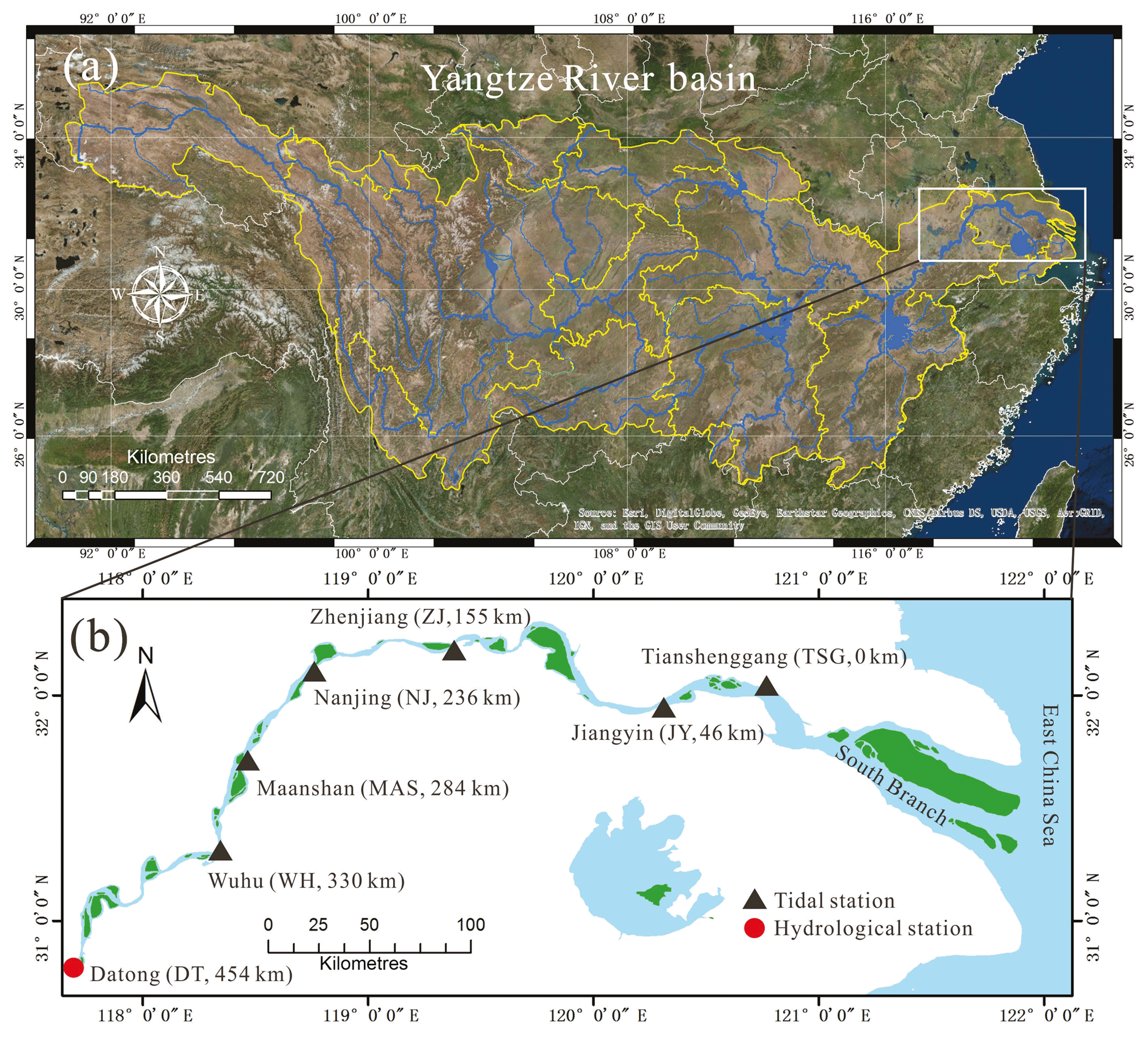
Figure 1Sketch map of the Yangtze River basin (a) and the Yangtze River estuary (b) displaying the location of gauging (triangle) and hydrological (circle) stations.
2.1 Description of the study site
The Yangtze River estuary, located on the east coast of China, extends ∼630 km from the Datong hydrological station (DT; the location of the tidal limit) to its mouth near the seaward end of the “South Branch” (Fig. 1). Both tidal waves and river flow are the major sources of energy for the hydrodynamics along the Yangtze River estuary. Specifically, the estuary is a meso-tidal coastal area with a maximum and mean tidal range of 4.62 and 2.67 m near the estuary mouth, respectively. The tide has an irregular semi-diurnal character with average flood and ebb durations of 5 and 7.5 h, respectively (Zhang et al., 2012). According to the observed data at DT (1950–2012), the annual mean river discharge is approximately 28 200 m3 s−1, and the monthly average river discharge reaches a maximum value of 49 500 m3 s−1 in July and a minimum value of 11 300 m3 s−1 in January. Unlike previous studies focusing on the tidal hydrodynamics near the estuary mouth, here we mainly concentrate on the tide–river dynamics in the mainstream of the Yangtze River estuary, extending from Tianshenggang gauging station to DT.
2.2 Datasets
Monthly averaged hydrological data (including tidal range and water level) from the following six tidal gauging stations along the Yangtze River estuary were collected from the Yangtze Hydrology Bureau of the People's Republic of China for the period from 2003 to 2014: Tianshenggang (TSG); Jiangyin (JY), located 46 km upstream of TSG; Zhenjiang (ZJ), located 155 km upstream of TSG; Nanjing (NJ), located 236 km upstream of TSG; Maanshan (MAS), located 284 km upstream of TSG; and Wuhu (WH), located 330 km upstream of TSG. The tidal amplitude was defined as half of the tidal range either during the flood or the ebb period, and we determined the mean value by averaging the tidal amplitudes during flood and ebb periods. To correctly calculate the residual water level slope, measured water levels from the gauging stations were corrected to the Yellow Sea 1985 vertical datum of local mean sea level. Figure 2 illustrates the temporal variation of the monthly averaged tidal range H and residual water level observed at the six gauging stations in addition to the monthly averaged river discharge observed at DT. In Fig. 2, we observe a strongly seasonal variation in H (except for TSG and JY) and due to the strongly fluctuating river discharge. For the residual water level, we also note that the further upstream the station, the more evident the seasonal change is.
3.1 Reproducing the residual water level profile in estuaries
The dynamics of the residual water level can be derived from the one-dimensional momentum equation (e.g. Savenije, 2005, 2012):
where U is the cross-sectional averaged velocity, Z is free surface elevation, h is water depth, g is the acceleration of gravity, t is time, ρ is water density, x is the longitudinal coordinate directed landward, and K is the Manning–Strickler friction coefficient. Assuming a periodic variation of flow velocity, the integration of Eq. (1) over a tidal cycle leads to an expression for the residual water level slope (e.g. Vignoli et al., 2003; Cai et al., 2014b, 2016):
where the over bars and the subscript zero indicate the tidal average and the value at the seaward boundary, respectively. As shown in Eq. (2), the residual water level slope is caused by three contributions made by residual friction, advective acceleration and density effects that correspond to the three terms on the right-hand side of Eq. (2). Note that the contribution from advective acceleration to the residual water level slope,
can be easily integrated to:
where we introduced the Froude number, , computed with the averaged variables. In this case, the correction is local (not cumulative) and proportional to the flow depth via a coefficient that is negligible as long as the velocity does not change significantly, and Fr is small, as is common for most tidal flows. With regard to the contribution from the density effect, it has been shown by Savenije (2005, 2012) that the induced value of the residual water level only amounts to around 1.25 % of the estuary depth over the salt intrusion length. Hence, in this study we neglect the impact of density on the dynamics of residual water level.
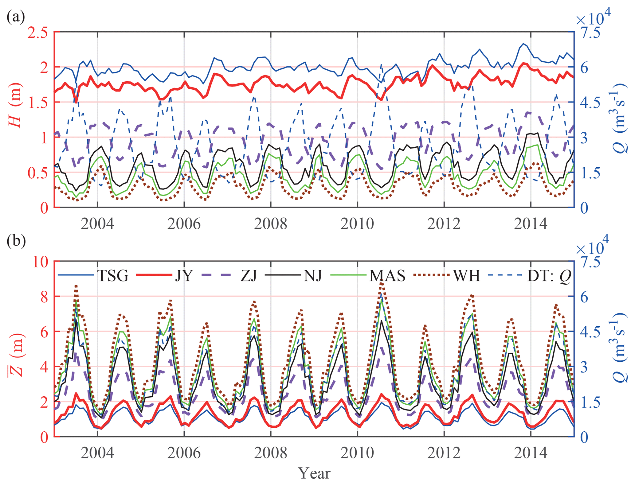
Figure 2Temporal (monthly averaged) variations of the observed tidal range, H, (a) and residual water level, , (b) at different gauging stations along the Yangtze River estuary and the observed river discharge at DT.
Assuming a negligible advective acceleration influence and density effect, integration of Eq. (2) leads to an expression for the residual water level:
if we assume at the estuary mouth (where x=0).
3.2 Analytical solution for tide–river dynamics
To correctly reproduce the residual water level profile in estuaries, an iterative procedure is required to properly calculate the friction term as presented in Eq. (5) as the velocity amplitude and water depth are unknown a priori. This is carried out using the analytical hydrodynamic model proposed by Cai et al. (2016). In the analytical model, the fundamental assumption made for the geometry of the estuary is that the tidally averaged cross-sectional area () and width () can be approximated by the following exponential functions (e.g. Cai et al., 2016):
where and are the respective cross-sectional area and width at the estuary mouth, and represent the respective asymptotic riverine cross-sectional area and width, and a and b denote the convergence lengths of the cross-sectional area and width, respectively. The tidally averaged depth () can be computed directly following the assumption of a mostly rectangular cross-section, i.e. . The possible impact of the lateral storage areas (e.g. tidal flats or salt marshes) can be described by the storage width ratio , defined as the ratio of the storage width BS and the tidally averaged stream width .
Table 1Dimensionless parameters adopted in the analytical model for tide–river dynamics.

Concentrating on a predominantly tidal constituent (e.g. M2) with frequency ω, it was shown by Cai et al. (2016) that tide–river dynamics are mainly determined by four externally defined, dimensionless parameters (see Table 1), i.e. the dimensionless tidal amplitude ζ defined as the ratio of the tidal amplitude to the depth, the estuary shape number γ (describing the cross-sectional area convergence), the friction number χ (representing the role of frictional dissipation), and the dimensionless river discharge φ (indicating the influence of freshwater discharge Q imposed at the upstream boundary), where η is the tidal amplitude, υ is the velocity amplitude, is the river flow velocity and c0 is the classical wave celerity in a prismatic frictionless channel, defined as .
The analytical solutions for the main tide–river dynamics can be obtained by solving a set of four implicit equations: the damping/amplification equation,
the phase lag equation,
the scaling equation,
and the celerity equation,
The main dependent dimensionless parameters in Eqs. (8)–(11) are presented in Table 1. They include the amplification/damping number δ, describing the rate of increase (δ>0) or decrease (δ<0) of the tidal wave amplitude along the channel axis; the velocity number μ, indicating the ratio of the actual velocity amplitude to the reference value in a prismatic frictionless channel; λ, the celerity number denoting the ratio of the classical wave celerity (c0) to the actual wave celerity (c), and ε, the phase lag between high water (HW) and high water slack (HWS) or between low water (LW) and low water slack (LWS), where ϕZ and ϕU are the water level phase and velocity, respectively. The unknown parameters θ, β and Γ in the damping/amplification equation account for the impact of river discharge, where θ and β are defined in Table 1, and Γ is given by
which is a friction factor derived by means of a Chebyshev polynomials approach (Cai et al., 2016). In Eq. (12), pi (i=0, 1, 2, 3) are the Chebyschev coefficients (see Dronkers, 1964, p.301), which are functions of the dimensionless river discharge φ through :
The set of Eqs. (8)–(11) can be regarded as a consistent analytical framework for understanding tide–river dynamics in estuaries. For more details about the computation procedure, readers can refer to Cai et al. (2014a, b, 2016).
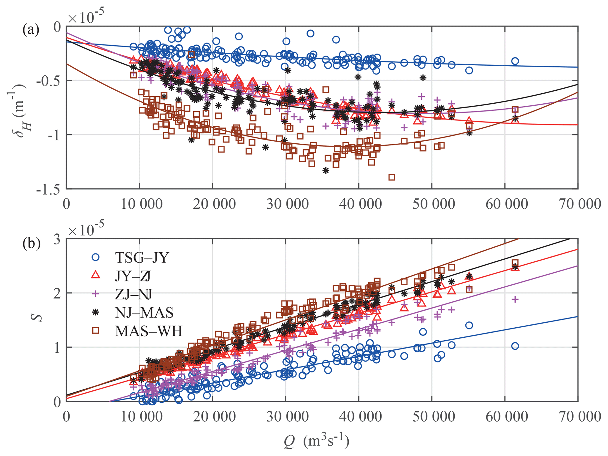
Figure 3Scatterplot and liner regression line of tidal damping rate, δH, (a) and residual water level slope, S, (b) for different reaches in the Yangtze River estuary as a function of river discharge observed at the DT hydrological station. Panel (a) also presents the quadratic regression lines, whereas panel (b) presents the linear regression lines.
4.1 Seasonal variation in tidal damping rate and residual water level slope
To understand the importance of seasonal changes in river discharge on tide–river dynamics, we first explore the seasonal variation of the tidal damping rate and the residual water level slope (Fig. 3). Here, the tidal damping rate (δH) and the residual water level slope (S) can be estimated for a reach of length Δx:
where η1 and are the tidal amplitude and residual water level on the seaward side, respectively, and η2 and are the corresponding values at a distance Δx upstream, respectively.
The study period covers tide–river dynamics under both low and high flow conditions, where the monthly average river discharge observed at DT ranges from approximately 9174 to 61 400 m3 s−1 so that the nonlinear interaction between tidal wave and river flow varies considerably. It has been previously shown that river discharge primarily impacts the tidal damping rate and residual water level slope via the friction term (Cai et al., 2014b, 2016). It can be clearly seen from Fig. 3 that both the tidal damping rate and residual water level slope vary strongly with river discharge. Remarkably, it appears that there is a threshold, corresponding to a critical value of river discharge, beyond which the relationship between the tidal damping rate and river discharge switches from negatively to positively correlated (Fig. 3a). This is particularly the case in the upper reach between the MAS and WH stations when the river discharge threshold is approximately 35 000 m3 s−1. The underlying mechanism will be elaborated upon further in Sect. 5.2. In Fig. 3b, it appears that the residual water level slope is linearly correlated with river discharge.
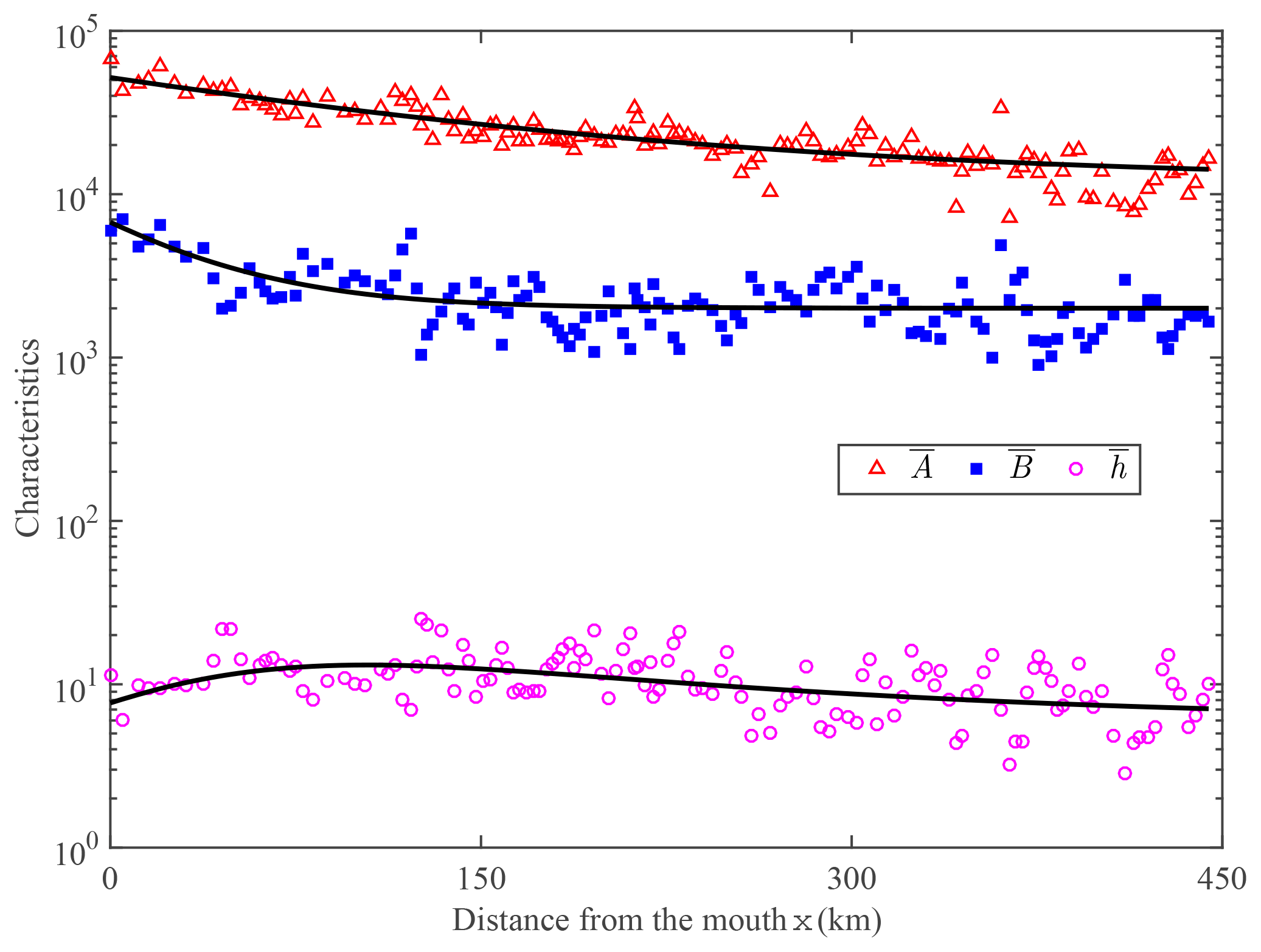
Figure 4Longitudinal variation of the main geometric characteristics (cross-sectional area, width and depth) along the Yangtze River estuary. The thick black lines represent the best-fitting curves.
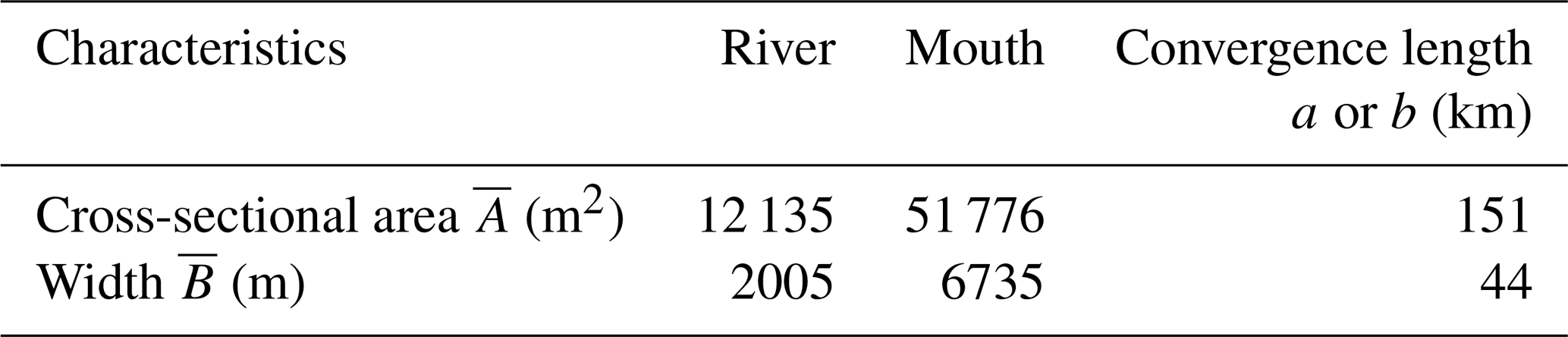
Table 2Characteristics of geometric parameters in the Yangtze River estuary.
4.2 Performance of the analytical model
The main geometric characteristics (including the tidally averaged cross-sectional area, width and depth) used in this paper were extracted from a digital elevation model (DEM) produced from Yangtze River estuary navigation charts surveyed in 2007. The elevations have been corrected to the local mean sea level of the Yellow Sea 1985 vertical datum. Figure 4 displays the longitudinal geometric quantities along the Yangtze River estuary axis, in combination with the best-fitting curves reproduced by Eqs. (6) and (7). Table 2 shows the calibrated geometric characteristics, where we observe a relatively large value of cross-sectional area convergence length (151 km), with a relatively small value for width (44 km), suggesting a fast transition from a funnel shaped reach to a prismatic reach in terms of width.
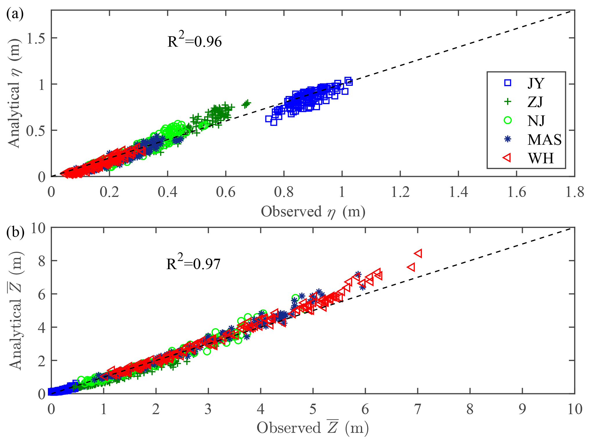
Figure 5Comparison of analytically computed tidal amplitude, η, (a) and residual water level, , (b) against the observations in the Yangtze River estuary during the study period (2003–2014).
The analytical model was calibrated and verified against the observed tidal amplitude and residual water level along the Yangtze River estuary on the basis of the monthly averaged hydrological data during the 2003–2014 period. The adopted seaward tidal amplitude (at TSG) and upward river discharge (at DT) in the analytical model are displayed in Fig. 2. As the Yangtze River estuary features a typical semi-diurnal character, for the sake of simplification, we used a typical M2 tidal period (i.e. 12.42 h). The only calibrated parameter in the analytical model is the Manning–Strickler friction coefficient K. The storage width ratio rS was assumed to be rS=1. The calibrated value of K was 80 m1∕3s−1 in the seaward region (x=0–32 km), whereas a smaller value of K=55 m1∕3s−1 was used in the river-dominated region (x=52–450 km). Meanwhile, in order to avoid a discontinuous jump caused by the adoption of different friction coefficients, we adopted a friction coefficient of K=80–55 m1∕3 s−1 (indicating a linear reduction of the friction coefficient) over the transitional reach (x=32–52 km). Figure 5 shows a comparison between the observed and computed tidal amplitude and residual water level at different gauging stations along the Yangtze River estuary for a wide range of tide and river discharge conditions. We observe that the correspondence between analytically computed results and observations is good with a high value for the coefficient of determination (R2>0.96), suggesting a reasonable performance of the analytical model for reproducing the first-order tide–river dynamics along the Yangtze River estuary. However, we note an overestimation of the analytically computed residual water level at upstream stations (i.e. MAS and WH) for values >5 m, which is likely due to the oversimplification of the geometry and flow characteristics (e.g. neglecting the M4 and M6 overtides) in the analytical model.
4.3 Seasonal behaviour of tide–river dynamics
The calibrated analytical model is subsequently used to explore the response of the main tide–river dynamics (represented by the damping/amplification number δ, the velocity number μ, the celerity number λ and the phase lag ε) to the seasonal variation of river discharge (Figs. 6 and S1–S3 in the Supplement). Figure 6a shows the spatial–temporal patterns of the damping number δ for the studied period (2003–2014), along with its minimum value δmin, which indicates the maximum tidal damping. The most noticeable feature of the spatial–temporal pattern of tidal damping is the seasonal variation with river discharge, which is clearly illustrated by the temporal variation of the tidal damping critical value δmin (see the red line in Fig. 6a, varying between 233 and 500 km in the Yangtze River estuary). To be more specific, in Fig. 6b, it can be observed that the critical value of tidal damping and its position along the estuary are negatively correlated with the corresponding river discharge. Generally, the critical value of tidal damping δmin reaches its minimum in December or January when the monthly average river discharge is minimum, and reaches its maximum in July with maximum river discharge throughout the year. Similarly, we observe that the position along the estuary with the critical δmin reaches its maximum value for minimum river discharge, and minimum value for maximum river discharge. Similar seasonal behaviour of velocity amplitude (denoted by the velocity number μ), wave celerity (denoted by the celerity number λ) and phase lag (denoted by ε) can also be reproduced using the calibrated analytical model (see Figs. S1–S3). In general, we observe a negatively correlated relation between μ, ε and Q, and a positively correlated relation between λ and Q.
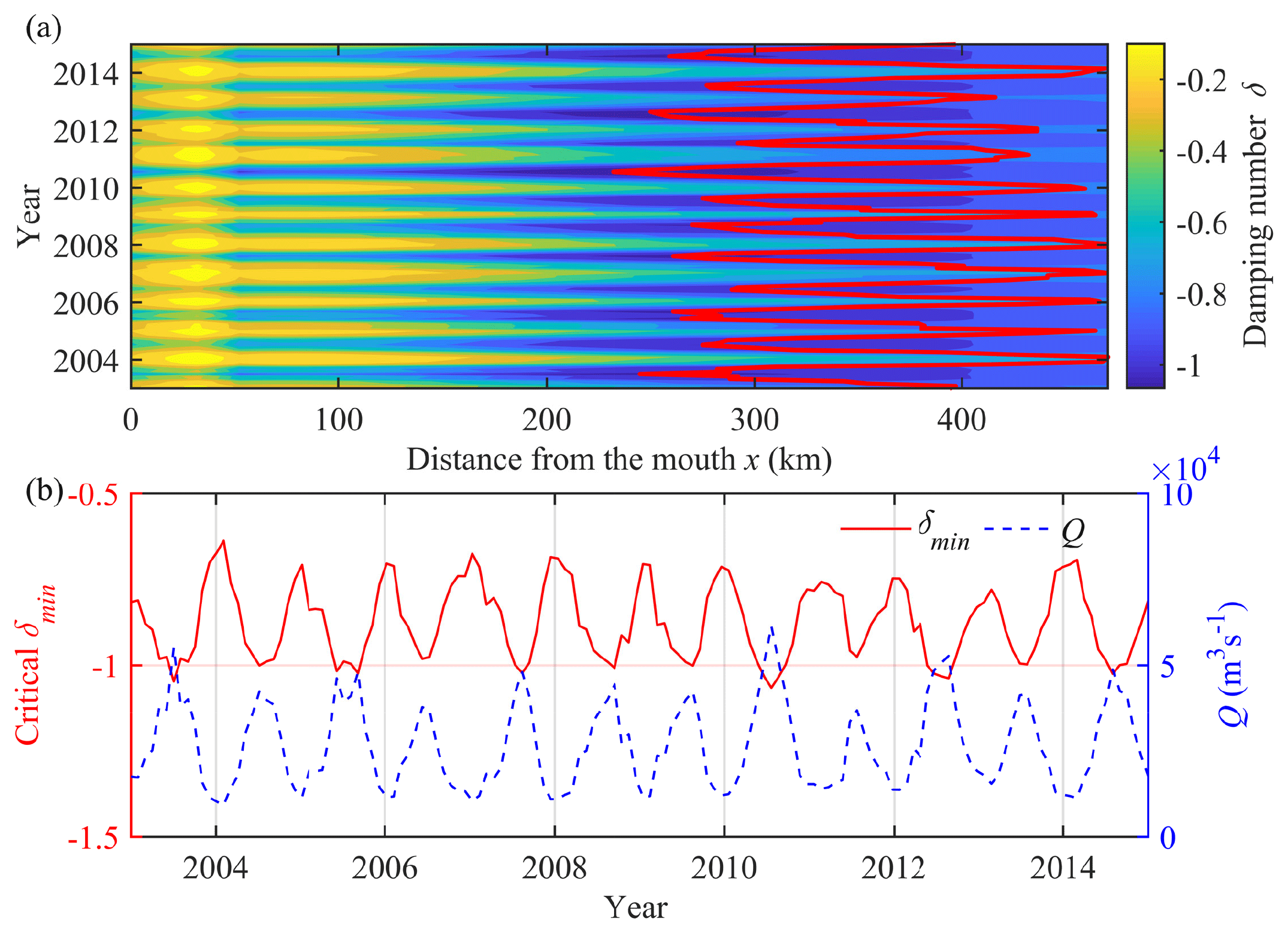
Figure 6Contour plot of the damping number δ and its minimum value δmin (indicated by the red line) for each month (a), and the relation between the critical value and river discharge Q (b).
4.4 Seasonal behaviour of the residual water level slope
For a typical tidal river, it is usually observed that the tidal range is reduced when the residual water level rises in the landward direction owing to the residual water level slope, which is mainly balanced by the residual frictional effect (Cai et al., 2014b, 2016). To understand the underlying mechanism of tidal wave propagation under the influence of river discharge, we adopted a decomposition method that can be used to quantify the contributions of tide, river and tide–river interaction to the residual water level slope S (see detailed derivation in Cai et al., 2016), computed as:
Equation (19) can be decomposed into three components contributing to the increase of the residual water level: a tidal component,
a riverine component,
and tide–river interaction component,
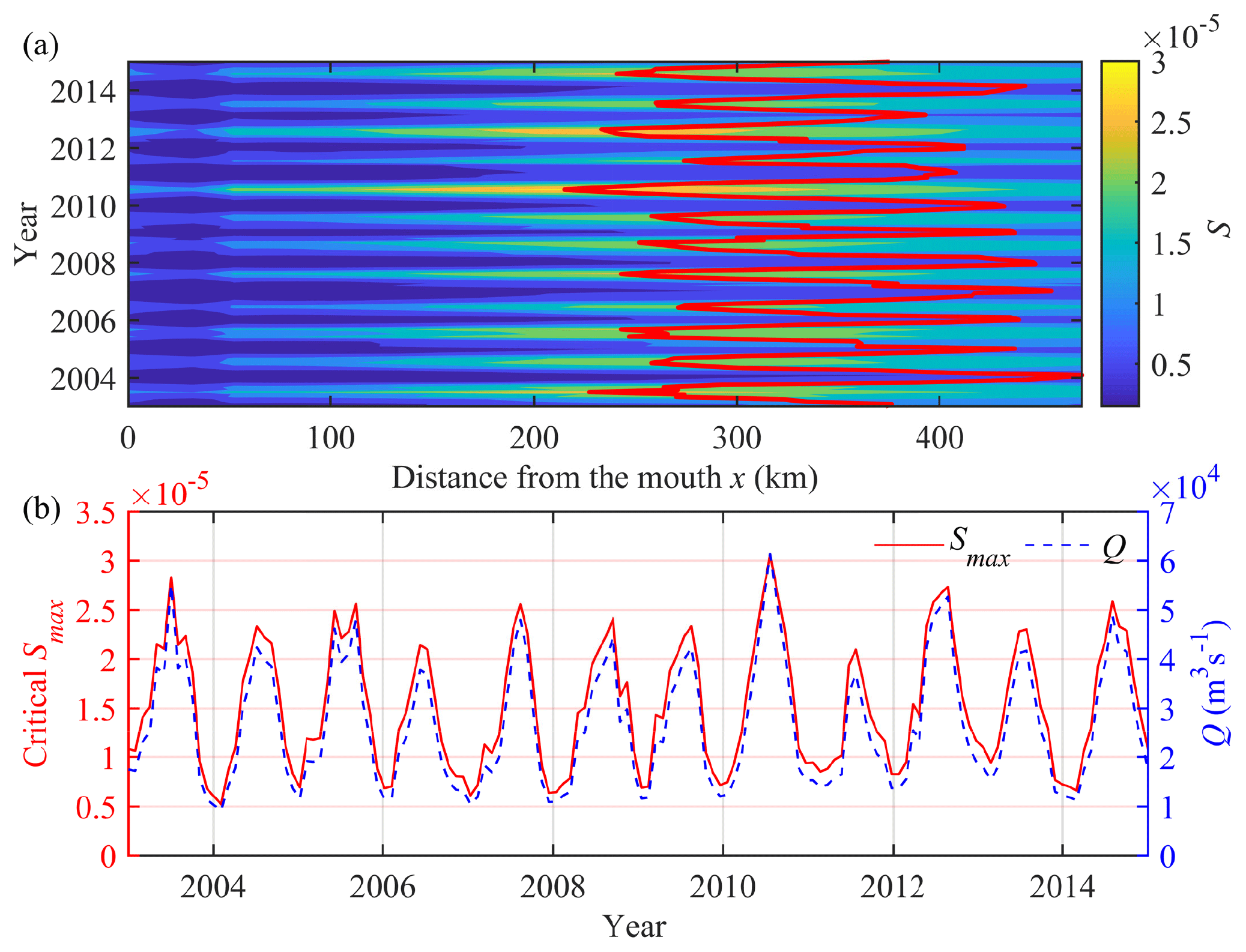
Figure 7Contour plot of the residual water level slope S and its minimum value Smax (indicated by the red line) for each month (a), and the relation between the critical value and river discharge Q (b).
Figure 7 shows the seasonal variation of the residual water level slope S, exhibiting a positively correlated relationship with the river discharge. It can be seen from Fig. 7a that the temporal variation of critical value Smax (maximum value) is quite similar to the tidal damping (see Fig. 6a), which suggests that the development of tide–river dynamics (e.g. tidal damping) is closely related to the residual water level slope. This indicates that both the maximum value of the residual water slope Smax (Fig. 7b) and its position along the estuary (Fig. 7a) are positively correlated with river discharge. To further understand the relative importance of tidal forcing alone, river flow alone and tide–river interactions, Eqs. (20)–(22) were used to quantify the contributions made by both tidal and riverine forcing. The results of these separate components are presented in Fig. S4, where we observe that the main contribution lies in the riverine component Sr. In addition, we note that the position of the maximum riverine component Sr is landward of the corresponding maximum values of the other two contributions (St and Str), which is mainly due to the relatively larger residual frictional effect introduced by the riverine forcing.
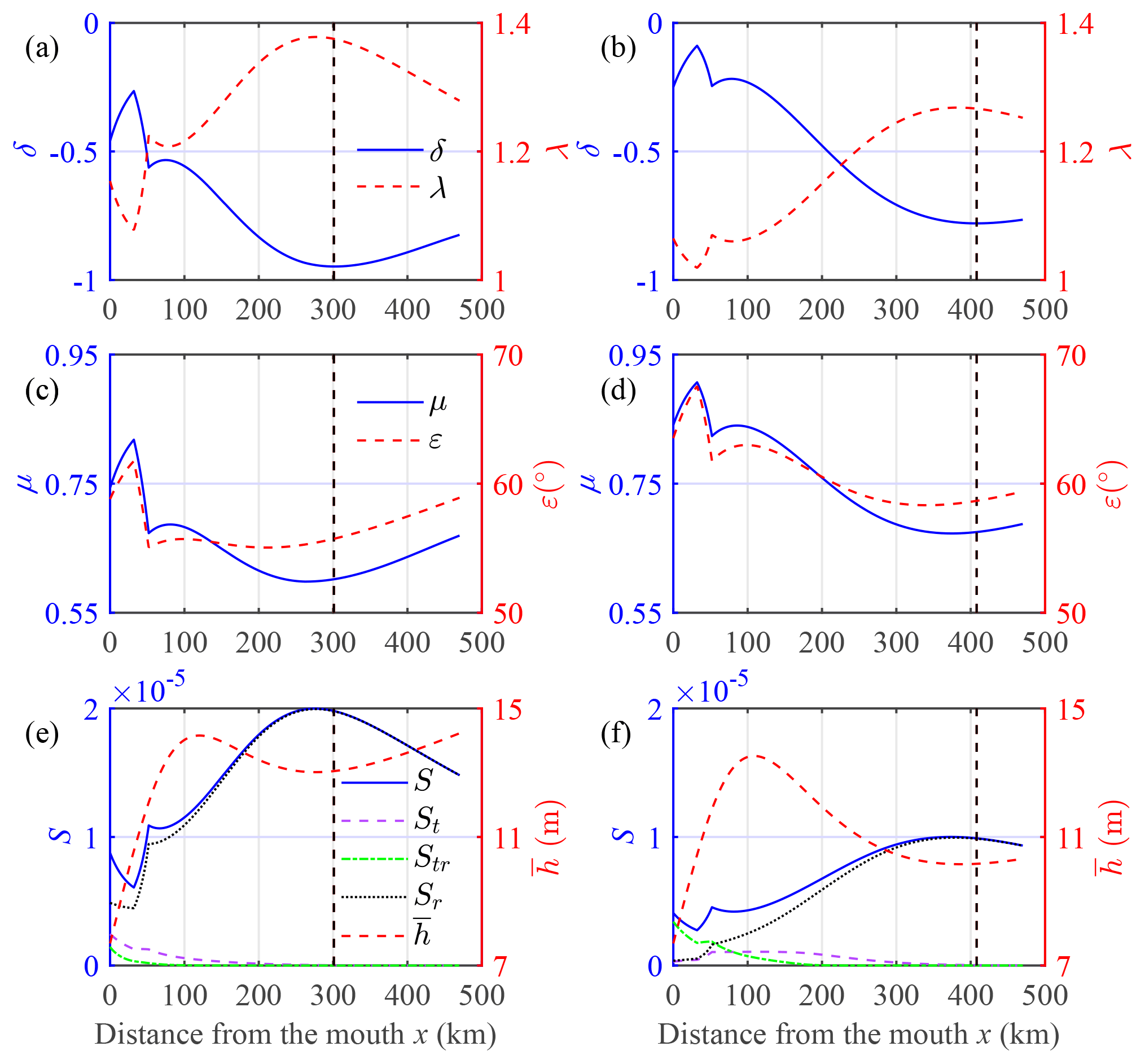
Figure 8Longitudinal variation of the main tide–river dynamics (a, b, c, d), as well as the contributions of tidal and riverine forcing to the residual water level slope and the water depth (e, f) for the wet (a, c, e) and dry seasons (b, d, f) in the Yangtze River estuary. The dashed lines in each sub-plot represent the critical position for maximum tidal damping (corresponding to the minimum value of damping number δ).
5.1 Critical position of maximum tidal damping (corresponding to the minimum value of damping number δ)
To understand the main processes that control the development of a maximum tidal damping, we used the average values of the observed tidal amplitude at TSG and the river discharge at DT as model inputs and reproduced the main tide–river dynamics along the Yangtze River estuary. Figure 8 shows the longitudinal variation of the main tidal dynamics (δ, λ, μ and ε) in addition to the contributions made by both tidal and riverine forcing to the residual water level slope and the water depth for both the wet (Fig. 8a, c, e) and dry (Fig. 8b, d, f) seasons. The discontinuous jump occurring at x=42 km depends on the adoption of different friction coefficients in the analytical model. Apparently, the critical position of maximum tidal damping is closer to the sea side during the wet season (around x=305 km) than during the dry season (around x=410 km) owing to the river discharge flush. In addition, the position of maximum tidal damping (corresponding to the minimum value of the damping number δ, indicated by the dashed black line) is almost coincident with the maximum value of the celerity number λ and the minimum value of the velocity number μ. The slightly lagged responses of λ and μ to δ are due to nonlinear interaction between these main tide–river dynamics parameters, as described by the set of nonlinear equations, Eqs. (8)–(11). This also indicates the significantly nonlinear effect caused by estuary shape, bottom friction and river discharge as the tidal wave propagates upriver. The change in phase lag ε directly follows from the phase lag equation (see Eq. 9). As can be seen from Fig. 8a–d, in general the phase lag ε is positively correlated with the damping number δ and the velocity number μ, whereas it is negatively correlated with the celerity number λ. Unlike tide-dominated estuaries with a negligible residual water level, the key parameter that determines the nonlinear relationship between the phase lag ε and the other variables (δ μ, λ) in tidal rivers lies in the water depth, which is controlled by the dynamics of the residual water level. The underlying mechanism generating the maximum tidal damping can be clearly shown in Fig. 8e and f, where we observe that the residual water level slope S and its dominant river component Sr increase to a maximum value near the critical position of maximum tidal damping, beyond which it is reduced. This means that the main tide–river dynamics are driven by the residual water level slope and that the critical position of maximum tidal damping is primarily controlled by the riverine forcing component. Furthermore, we also note that the maximum value of S corresponds to the local minimum , which suggests a dominant impact of residual water level (and hence water depth) on tide–river dynamics in the Yangtze River estuary.
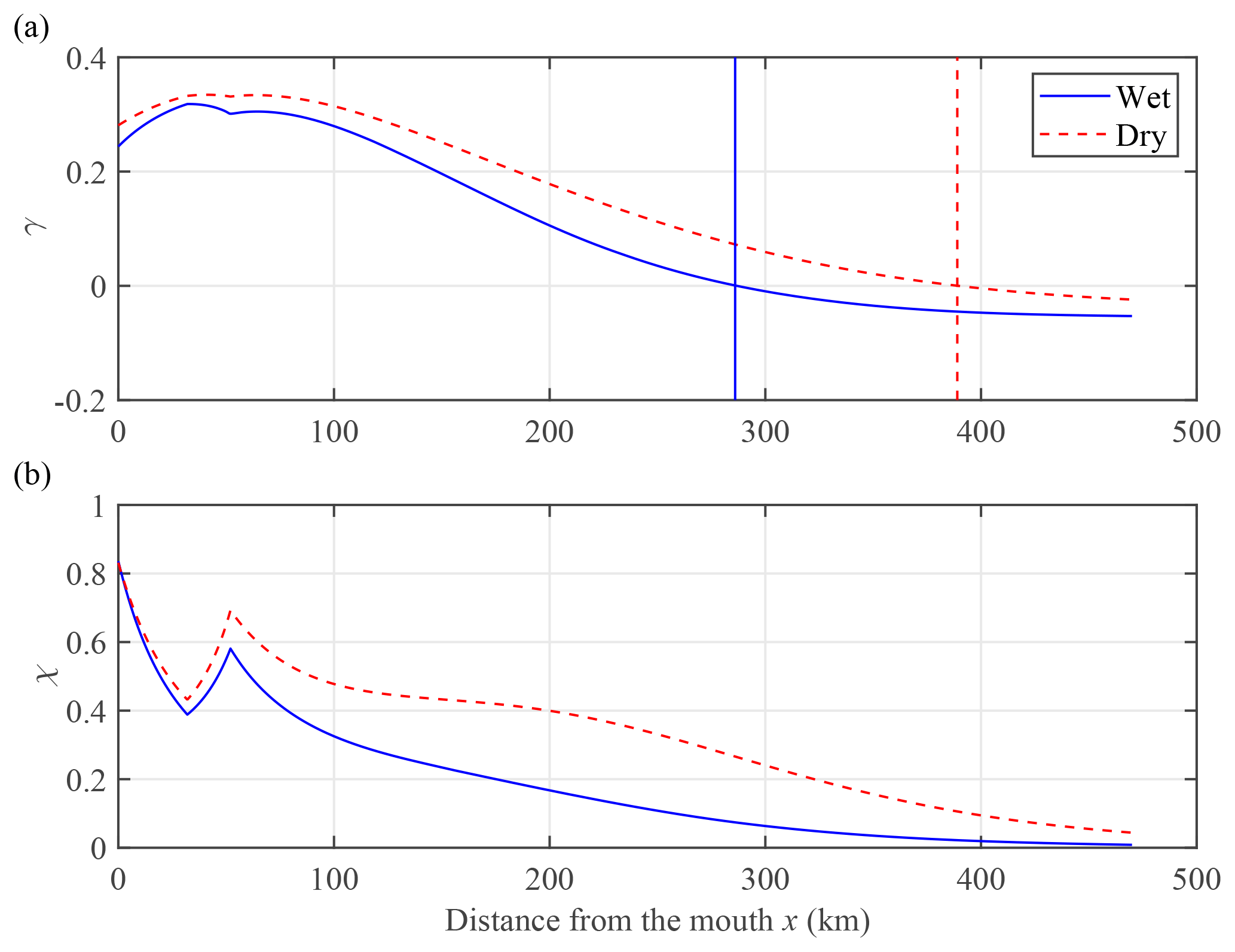
Figure 9Longitudinal variation of the estuary shape number γ (a) and the friction number χ (b) for the wet and dry seasons in the Yangtze River estuary. Panel (a) also indicates the position of the critical value of channel convergence (i.e. γ=0) using the corresponding lines for the wet and dry seasons.
It is also worth examining the longitudinal and seasonal variations of the two controlling parameters represented by the estuary shape number γ and the friction number χ (see Fig. 9), which are closely related to the strength of tidal damping δ. Remarkably, it is important to note that the effect of channel convergence (represented by γ) is stronger during the dry season (larger value of γ) than during the wet season. This indicates that river discharge also tends to reduce the channel convergence via the generation of the residual water level slope. In addition, we observe a switch of γ from positive to negative at x=290 km and x=394 km for the wet and dry seasons, respectively (Fig. 9a). The cause of the negative value for γ is that the cross-sectional area increases in the landward direction (hence ) owing to the increasing residual water level and depth. In Fig. 9b, we observe a larger value for the friction number χ during the dry season than during the wet season, which is mainly due to the relatively larger tidal amplitude during the dry season and the residual water level (hence the water depth) increasing with river discharge (see the definition of χ in Table 1). Furthermore, it is also noted that χ asymptotically approaches zero with distance. This means that in the upstream part of the estuary tide–river dynamics are primarily determined by the geometric effect (i.e. the divergence of the cross-sectional area) and the residual frictional effect caused by riverine forcing Sr (see Eq. 21).
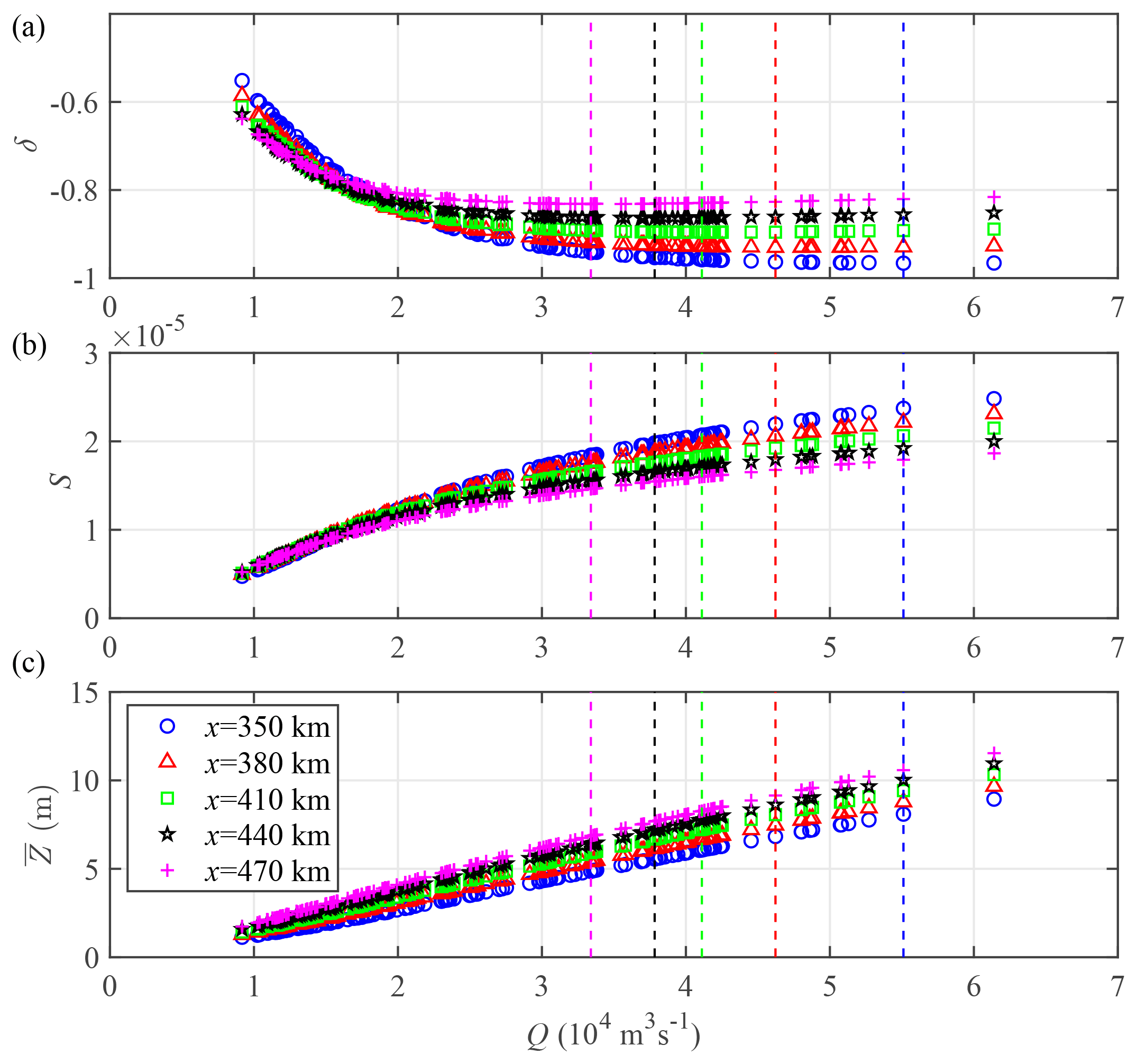
Figure 10Relationship between the tidal damping number δ (a), the residual water level slope S (b), the residual water level (c) and the corresponding river discharge Q imposed at DT for different positions, indicated by different symbols. The dashed lines that are the same colour as the symbols are used to identify the critical river discharge for the maximum tidal damping (corresponding to the minimum value of δ in a).
5.2 Critical river discharge for maximum tidal damping
Based on the analytical results, in Fig. 10 we display how the tidal damping δ, the residual water level slope S and the residual water level develop as a function of river discharge Q for different positions in the upstream river-dominated region, where the maximum tidal damping occurs. Figure 10a shows the tidal damping at different positions with different river discharges. It also displays the critical value of river discharge corresponding to maximum tidal damping. As expected, more river discharge is required to change tidal damping from a negative gradient (indicating a strengthening damping with respect to river discharge Q) to a positive gradient (indicating a weakening damping with respect to river discharge Q) for the seaward positions where tide exerts more influence. The critical river discharge is approximately 34 000 m3 s−1 at x=470 km, and it gradually increases to 55 000 m3 s−1 at x=350 km. In Fig. 10a, we also note that beyond the critical value of maximum damping the δ appears to slightly increase until an asymptotic value is approached. Figure 10b and c show the relation between S, and Q. It is noticeable that the curves for residual water level appear as straight lines, corresponding to a consistent increase of the residual water level slope S with river discharge Q. Unlike the longitudinal variation of the maximum S value (see Fig. 8e, f), both S and monotonously increase with Q. In addition, it can be seen from Fig. 10a that a threshold of approximately 15 000 m3 s−1 exists for the tidal damping with respect to the position along the estuary. At lower river discharges (Q<15 000 m3 s−1), the damping number δ tends to decrease (indicating a strengthening damping) in the landward direction, whereas opposite is seen at higher river discharges (Q>15 000 m3 s−1).
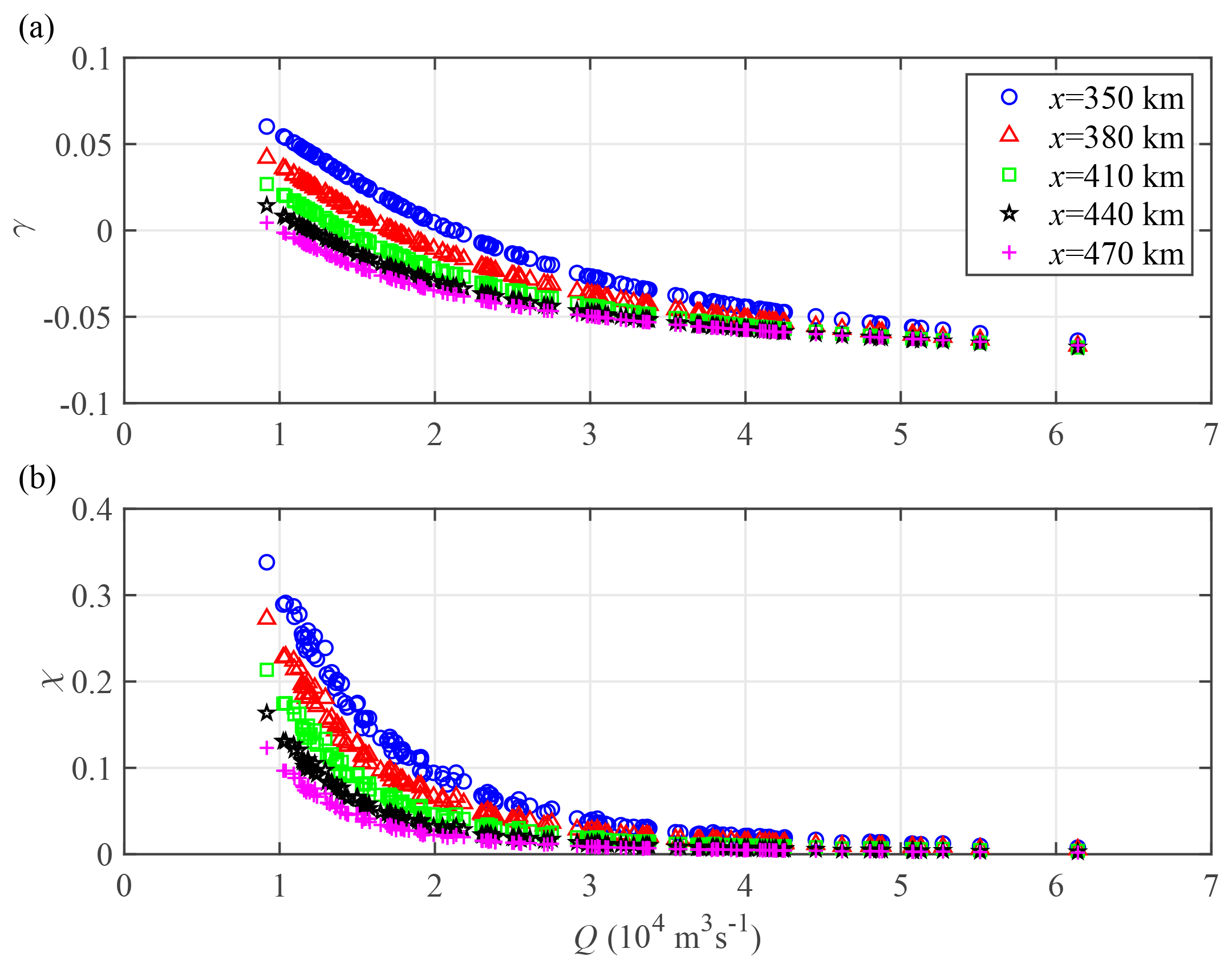
Figure 11Relationship between the estuary shape number γ (a), the friction number χ (b) and the river discharge Q.
The underlying mechanism for achieving a critical river discharge for maximum tidal damping can be primarily attributed to the cumulative effect of the residual water level altering the water depth and hence the channel convergence and effective friction, according to the definitions of the estuary shape number γ and the friction number χ in Table 1. Figure 11 presents these two controlling parameters (γ and χ) as a function of river discharge Q. It can be clearly seen in Fig. 11a that there is an apparent switch of the estuary shape number γ from positive (indicating a reduction of cross-sectional area in the landward direction) to negative (indicating an increase of cross-sectional area in the landward direction). In addition, more river discharge is required to achieve a switch in the estuary shape number γ for the seaward positions where tide exerts more influence. The main reason for such a switch is the consistent increase of the residual water level and, in turn, the water depth and cross-sectional area with river discharge. Conversely, the effective friction induced by tidal forcing (represented by χ) asymptotically approaches zero with the river discharge (see Fig. 11b), which suggests that the estuarine system is primarily controlled by the divergence of the cross-sectional area and the residual frictional effect caused by riverine forcing (represented by Sr in Eq. 21) for high river discharge conditions. Additionally, we can conclude that the asymptotic behaviour of tidal damping δ with high river discharge (as shown in Fig. 10a) is due to the corresponding asymptotic behaviour of the estuary shape number γ and the friction number χ (and hence the residual frictional effect indicated by S as presented in Fig. 10b).
5.3 Model limitation and transferability
Although the current analytical model can reproduce the first-order tide–river dynamics well, it also has some limitations. The fundamental assumption is that the tidal wave can be described by a combination of a steady residual term (generated by the river discharge) and a time-dependent harmonic wave (introduced by the tidal flow). Thus, the proposed model can only capture the tidal asymmetry caused by tide–river interaction while it neglects the tidal asymmetry introduced by astronomical tides (e.g. nonlinear interactions among K1, O1 and M2), overtides (e.g. M4) and compound tides (e.g. MSf). Consequently, the proposed analytical method is preferably applied to tidal rivers with a predominant tidal constituent (e.g. M2 or K1).
It is assumed that both the tidally averaged cross-sectional area and channel width can be approximated by exponential functions following Eqs. (6)–(7). However, this is not a restrictive assumption as the model can, in principle, be applied to an arbitrary estuarine shape (i.e. bed elevation and channel width), as long as the variation of the cross-section is gradual. The proposed model can also be used to quantify the spring–neap variability of the tide–river dynamics based on daily averaged tidal amplitude and river discharge conditions (see example in Cai et al., 2016). However, the model cannot be used to explore the tide–river dynamics within a tidal cycle as it is based on a tidally averaged scale. This means that it may not be applicable to the cases with rapidly varying river discharge.
5.4 Implications for sustainable water management and sediment transport
Knowledge of the development and evolution of tide–river dynamics that determine the behaviour of tidal damping and residual water level slope under external forcing (e.g. tidal and riverine flow) and geometry changes (e.g. deepening and land reclamation) are essential for improving the sustainable water management in estuaries. Adopting the method proposed in this study, one can evaluate the influence of human intervention on the estuarine system (such as large-scale sand excavation, dredging for navigational channels or freshwater withdrawal), on flood control structures (e.g. storm surge barriers, flood gates) and on the aquatic environment (e.g. such as salt intrusion and the related water quality). For instance, Cai et al. (2019) explored how the freshwater regulation of the Three Gorges Dam (the world's largest hydroelectric station in terms of installed power capacity) may affect the alteration of the tidal limit in the Yangtze River estuary using the analytical model proposed in this paper. It was shown that the largest change of the tidal limit of around 75 km occurred in October owing to the substantial increase in freshwater discharge. When combined with ecological or salt intrusion models, the analytical approach presented in this study is particularly useful for a quick computation of the longitudinal distribution of the salinity (e.g. Cai et al., 2015). Using salinity as a general predictor, it is possible to assess the potential impacts of human intervention on the aquatic ecosystem health in general (e.g., water quality, water utilisation and agricultural development in the estuarine area).
As tide propagates into an estuary, it is distorted and becomes asymmetric due to significant nonlinear interactions with geometry and river flow. Tidal asymmetry is regarded as one of the most important mechanisms generating residual sediment transport (e.g. Friedrichs and Aubrey, 1988; Parker, 1991; Guo et al., 2014, 2015, 2016; Zhang et al., 2018b). Although the current analytical method can only deal with tide–river interaction for a single predominant tidal constituent (e.g. M2), the model does capture the major tidal asymmetry induced by geometric effect and riverine flow (e.g. the tidal asymmetry caused by the residual river flow) and can reproduce the seasonal behaviour of tidal damping and residual water level slope well. It was shown by Lamb et al. (2012) that the erosion and deposition patterns along an estuary are strongly related to the shape of the residual water level profile, which we have shown to be linked to the tide–river dynamics and the geometry of the estuary. The successful reproduction of the seasonal behaviour of tide–river dynamics and residual water level slope in the Yangtze River estuary suggests that the proposed analytical approach can be used as a tool for detecting the evolution of estuarine morphology under various external forcing conditions. However, further studies are required to quantify the relationship between the residual water level slope and the estuarine morphology.
Both observations and analytical model results show a critical value of river discharge that causes maximum tidal damping in the upstream part of the tidal river, challenging the concept of how river discharge dampens tidal waves. The residual water level slope, mainly balanced by the residual frictional effect, plays a key role in determining the evolution of tide–river dynamics under a wide range of tidal and riverine forcing conditions. A critical position along the estuary is where there is maximum tidal damping, upstream of which the residual water level slope is reduced. The location of this position moves seaward with an increase in river discharge. From that position landwards, the effect of river discharge on tidal damping becomes weaker instead of stronger, indicating a weakening of the backwater effect induced by the residual frictional effect. It is worth noting that the underlying mechanism of generating critical position along the estuary is similar to that of generating critical river discharge due to the fact that for a given (constant) river discharge, the effect caused by river discharge becomes stronger with distance upstream in a tidal river, which is analogous to a river discharge increase at a given (fixed) location.
Moreover, analytical model results show that more river discharge is required to change the maximum tidal damping critical value from a negative to a positive gradient for the seaward positions where the tide exerts stronger impact. The underlying mechanism has to do with the fact that river discharge affects tidal damping: on the one hand, attenuating tidal motion by increasing the quadratic velocity in the numerator, and on the other hand, reducing the effective friction by increasing the water depth in the denominator. The occurrence of critical river discharge suggests the cumulative effect of the residual water level (increasing the water depth and the cross-sectional area) that exceeds the threshold of tide–river dynamics, beyond which tidal damping weakens with river discharge. To the best of our knowledge, this is one of the few studies that shows the gradient switch of the cross-sectional area (i.e. ) and tidal damping (i.e. dδ∕dx) with the river discharge, shedding new light on the impact of river discharge on tidal damping in alluvial estuaries (see also Matte et al., 2018, 2019). Moreover, the results obtained in this study will, hopefully, provide scientific guidelines for water resources management (e.g. flood control and salt intrusion prevention) in the Yangtze River estuary and other tidal rivers worldwide.
All of the data used in this study were obtained from the source mentioned in Sect. 2.
The supplement related to this article is available online at: https://doi.org/10.5194/hess-23-2779-2019-supplement.
All authors contributed to the design and development of the work. The experiments were originally carried out by HC. XZ, LG and MZ carried out the data analysis. FL and HC prepared the paper with contributions from all co-authors. HHGS, EG and QY reviewed the paper.
The authors declare that they have no conflict of interest.
The authors thank the two anonymous referees for their constructive comments and suggestions, which have greatly improved the quality of this paper.
This research has been supported by the Open Research Fund of the State Key Laboratory of Estuarine and Coastal Research (grant no. SKLEC-KF201809), the National Natural Science Foundation of China (grant nos. 51709287, 41106015, 41476073, 41506105 and 41876091), the Basic Research Program of Sun Yat-Sen University (grant no. 17lgzd12) and the Guangdong Provincial Natural Science Foundation of China (grant no. 2017A030310321). The work of Erwan Garel was supported by a FCT research contract (IF/00661/2014/CP1234).
This paper was edited by Insa Neuweiler and reviewed by two anonymous referees.
Alebregtse, N. C. and de Swart, H. E.: Effect of river discharge and geometry on tides and net water transport in an estuarine network, an idealized model applied to the Yangtze Estuary, Cont. Shelf. Res., 123, 29–49, https://doi.org/10.1016/j.csr.2016.003.028, 2016. a, b, c, d, e
Buschman, F. A., Hoitink, A. J. F., van der Vegt, M., and Hoekstra, P.: Subtidal water level variation controlled by river flow and tides, Water Resour. Res., 45, W10420, https://doi.org/10.1029/2009WR008167, 2009. a, b, c
Cai, H., Savenije, H. H. G., and Toffolon, M.: A new analytical framework for assessing the effect of sea-level rise and dredging on tidal damping in estuaries, J. Geophys. Res., 117, C09023, https://doi.org/10.1029/2012JC008000, 2012a. a
Cai, H., Savenije, H. H. G., Yang, Q., Ou, S., and Lei, Y.: Influence of river discharge and dredging on tidal wave propagation: Modaomen Estuary case, J. Hydraul. Eng., 138, 885–896, https://doi.org/10.1061/(ASCE)HY.1943-7900.0000594, 2012b. a, b
Cai, H., Savenije, H. H. G., and Jiang, C.: Analytical approach for predicting fresh water discharge in an estuary based on tidal water level observations, Hydrol. Earth Syst. Sci., 18, 4153–4168, https://doi.org/10.5194/hess-18-4153-2014, 2014a. a, b, c, d
Cai, H., Savenije, H. H. G., and Toffolon, M.: Linking the river to the estuary: influence of river discharge on tidal damping, Hydrol. Earth Syst. Sci., 18, 287–304, https://doi.org/10.5194/hess-18-287-2014, 2014b. a, b, c, d, e, f, g, h, i, j, k, l, m, n
Cai, H., Savenije, H. H. G., Zuo, S., Jiang, C., and Chua, V.: A predictive model for salt intrusion in estuaries applied to the Yangtze estuary, J. Hydrol., 529, 1336–1349, https://doi.org/10.1016/j.jhydrol.2015.08.050, 2015. a
Cai, H., Savenije, H. H. G., Jiang, C., Zhao, L., and Yang, Q.: Analytical approach for determining the mean water level profile in an estuary with substantial fresh water discharge, Hydrol. Earth Syst. Sci., 20, 1177–1195, https://doi.org/10.5194/hess-20-1177-2016, 2016. a, b, c, d, e, f, g, h, i, j, k, l, m, n, o, p, q, r, s, t, u
Cai, H., Yang, Q., Zhang, Z., Guo, X., Liu, F., and Ou, S.: Impact of river-tide dynamics on the temporal-spatial distribution of residual water levels in the Pearl River channel networks, Estuar. Coast, 41, 1885–1903, https://doi.org/10.1007/s12237-018-0399-2, 2018. a
Cai, H., Zhang, X., Zhang, M., Guo, L., Liu, F., and Yang, Q.: Impacts of Three Gorges Dam's operation on spatial–temporal patterns of tide–river dynamics in the Yangtze River estuary, China, Ocean Sci., 15, 583–599, https://doi.org/10.5194/os-15-583-2019, 2019. a
Dronkers, J. J.: Tidal computations in River and Coastal Waters, Elsevier, New York, 1–518, 1964. a, b, c
Friedrichs, C. T. and Aubrey, D. G.: Non-linear tidal distortion in shallow well-mixed estuaries: A synthesis, Estuar. Coast Shelf S., 27, 521–545, https://doi.org/10.1016/0272-7714(88)90082-0, 1988. a
Godin, G.: Modification of River Tides by the Discharge, J. Waterw. Port C-Asce, 111, 257–274, https://doi.org/10.1061/(ASCE)0733-950X(1985)111:2(257), 1985. a, b
Godin, G.: Compact Approximations to the Bottom Friction Term, for the Study of Tides Propagating in Channels, Cont. Shelf. Res., 11, 579–589, https://doi.org/10.1016/0278-4343(91)90013-V, 1991. a
Godin, G.: The propagation of tides up rivers with special considerations on the upper Saint Lawrence river, Estuar. Coast Shelf S., 48, 307–324, https://doi.org/10.1006/ecss.1998.0422, 1999. a, b, c
Godin, G. and Martinez, A.: Numerical Experiments to Investigate the Effects of Quadratic Friction on the Propagation of Tides in a Channel, Cont. Shelf. Res., 14, 723–748, https://doi.org/10.1016/0278-4343(94)90070-1, 1994. a
Guo, L., van der Wegen, M., Roelvink, J. A., and He, Q.: The role of river flow and tidal asymmetry on 1-D estuarine morphodynamics, J. Geophys. Res., 119, 2315–2334, https://doi.org/10.1002/2014JF003110, 2014. a, b
Guo, L., van der Wegen, M., Jay, D. A., Matte, P., Wang, Z. B., Roelvink, D. J., and He, Q.: River-tide dynamics: Exploration of non-stationary and nonlinear tidal behavior in the Yangtze River estuary, J. Geophys. Res., 120, 3499–3521, https://doi.org/10.1002/2014JC010491, 2015. a, b, c, d, e, f
Guo, L. C., van der Wegen, M., Wang, Z. B., Roelvink, D., and He, Q.: Exploring the impacts of multiple tidal constituents and varying river flow on long-term, large-scale estuarine morphodynamics by means of a 1-D model, J. Geophys. Res., 121, 1000–1022, https://doi.org/10.1002/2016JF003821, 2016. a, b
Hoitink, A. J. F. and Jay, D. A.: Tidal river dynamics: Implications for deltas, Rev. Geophys., 54, 240–272, https://doi.org/10.1002/2015RG000507, 2016. a
Hoitink, A. J. F., Wang, Z. B., Vermeulen, B., Huismans, Y., and Kastner, K.: Tidal controls on river delta morphology, Nat. Geosci., 10, 637–645, https://doi.org/10.1038/ngeo3000, 2017. a
Horrevoets, A. C., Savenije, H. H. G., Schuurman, J. N., and Graas, S.: The influence of river discharge on tidal damping in alluvial estuaries, J. Hydrol., 294, 213–228, https://doi.org/10.1016/j.jhydrol.2004.02.012, 2004. a, b
Jay, D. A.: Green Law Revisited – Tidal Long-Wave Propagation in Channels with Strong Topography, J. Geophys. Res., 96, 20585–20598, https://doi.org/10.1029/91JC01633, 1991. a
Jay, D. A. and Flinchem, E. P.: Interaction of fluctuating river flow with a barotropic tide: A demonstration of wavelet tidal analysis methods, J. Geophys. Res., 102, 5705–5720, https://doi.org/10.1029/96JC00496, 1997. a
Jay, D. A. and Flinchem, E. P.: A comparison of methods for analysis of tidal records containing multi-scale non-tidal background energy, Cont. Shelf. Res., 19, 1695–1732, https://doi.org/10.1016/S0278-4343(99)00036-9, 1999. a
Jay, D. A., Leffler, K., and Degens, S.: Long-Term Evolution of Columbia River Tides, J. Waterw. Port C-Asce, 137, 182–191, https://doi.org/10.1061/(ASCE)WW.1943-5460.0000082, 2011. a, b
Jay, D. A., Leffler, K., Diefenderfer, H. L., and Borde, A. B.: Tidal-Fluvial and Estuarine Processes in the Lower Columbia River: I. Along-Channel Water Level Variations, Pacific Ocean to Bonneville Dam, Estuar. Coast, 38, 415–433, https://doi.org/10.1007/s12237-014-9819-0, 2015. a
Kuang, C., Chen, W., Gu, J., Su, T., Song, H., Ma, Y., and Dong, Z.: River discharge contribution to sea-level rise in the Yangtze River Estuary, China, Cont. Shelf. Res., 134, 63–75, https://doi.org/10.1016/j.csr.2017.01.004, 2017. a
Kukulka, T. and Jay, D. A.: Impacts of Columbia River discharge on salmonid habitat: 1. A nonstationary fluvial tide model, J. Geophys. Res., 108, 3293 https://doi.org/10.1029/2002JC001382, 2003a. a, b
Kukulka, T. and Jay, D. A.: Impacts of Columbia River discharge on salmonid habitat: 2. Changes in shallow-water habitat, J. Geophys. Res., 108, 3294 https://doi.org/10.1029/2003JC001829, 2003b. a
Lamb, M. P., Nittrouer, J. A., Mohrig, D., and Shaw, J.: Backwater and river plume controls on scour upstream of river mouths: Implications for fluvio-deltaic morphodynamics, J. Geophys. Res., 117, F01002, https://doi.org/10.1029/2011JF002079, 2012. a, b
LeBlond, P. H.: Forced fortnightly tides in shallow waters, Atmos. Ocean, 17, 253–264, https://doi.org/10.1080/07055900.1979.9649064, 1979. a, b
Leonardi, N., Kolker, A. S., and Fagherazzi, S.: Interplay between river discharge and tides in a delta distributary, Adv. Water Resour., 80, 69–78, https://doi.org/10.1016/j.advwatres.2015.03.005, 2015. a, b
Lu, S., Tong, C., Lee, D. Y., Zheng, J., Shen, J., Zhang, W., and Yan, Y.: Propagation of tidal waves up in Yangtze Estuary during the dry season, J. Geophys. Res., 120, 6445–6473, https://doi.org/10.1002/2014JC010414, 2015. a
Matte, P., Jay, D. A., and Zaron, E. D.: Adaptation of Classical Tidal Harmonic Analysis to Nonstationary Tides, with Application to River Tides, J. Atmos. Ocean Tech., 30, 569–589, https://doi.org/10.1175/Jtech-D-12-00016.1, 2013. a
Matte, P., Secretan, Y., and Morin, J.: Temporal and spatial variability of tidal-fluvial dynamics in the St. Lawrence fluvial estuary: An application of nonstationary tidal harmonic analysis, J. Geophys. Res., 119, 5724–5744, https://doi.org/10.1002/2014JC009791, 2014. a
Matte, P., Secretan, Y., and Morin, J.: Reconstruction of Tidal Discharges in the St. Lawrence Fluvial Estuary: The Method of Cubature Revisited, J. Geophys. Res., 123, 5500–5524, https://doi.org/10.1029/2018JC013834, 2018. a, b
Matte, P., Secretan, Y., and Morin, J.: Drivers of residual and tidal flow variability in the St. Lawrence fluvial estuary: Influence on tidal wave propagation, Cont. Shelf. Res., 174, 158–173, https://doi.org/10.1016/j.csr.2018.12.008, 2019. a, b
Parker, B. B.: The relative importance of the various nonlinear mechanisms in a wide range of tidal interactions, in: Tidal Hydrodynamics, edited by: Parker, B., John Wiley and Sons, Hoboken, N. J., 237–268, 1991. a
Sassi, M. G. and Hoitink, A. J. F.: River flow controls on tides and tide-mean water level profiles in a tidal freshwater river, J. Geophys. Res., 118, 4139–4151, https://doi.org/10.1002/Jgrc.20297, 2013. a, b, c
Savenije, H. H. G.: Salinity and Tides in Alluvial Estuaries, Elsevier, New York, 1–194, 2005. a, b, c
Savenije, H. H. G.: Salinity and Tides in Alluvial Estuaries, completely revised 2 Edn, https://salinityandtides.com/ (last access: 10 June 2015), 2012. a, b, c, d
Savenije, H. H. G., Toffolon, M., Haas, J., and Veling, E. J. M.: Analytical description of tidal dynamics in convergent estuaries, J. Geophys. Res., 113, C10025, https://doi.org/10.1029/2007JC004408, 2008. a
Shi, S., Cheng, H., Xuan, X., Hu, F., Yuan, X., Jiang, Y., and Zhou, Q.: Fluctuations in the tidal limit of the Yangtze River estuary in the last decade, Sci. China Earth Sci., 8, 1136–1147, https://doi.org/10.1007/s11430-017-9200-4, 2018. a, b
Vignoli, G., Toffolon, M., and Tubino, M.: Non-linear frictional residual effects on tide propagation, in: Proceedings of XXX IAHR Congress, Vol. A, 24–29 August 2003, Thessaloniki, Greece, 291–298, 2003. a
Zhang, E. F., Savenije, H. H. G., Chen, S. L., and Mao, X. H.: An analytical solution for tidal propagation in the Yangtze Estuary, China, Hydrol. Earth Syst. Sci., 16, 3327–3339, https://doi.org/10.5194/hess-16-3327-2012, 2012. a
Zhang, F., Sun, J., Lin, B., and Huang, G.: Seasonal hydrodynamic interactions between tidal waves and river flows in the Yangtze Estuary, J. Mar. Syst., 186, 17–28, https://doi.org/10.1016/j.jmarsys.2018.05.005, 2018a. a, b, c, d
Zhang, M., Townend, I., Cai, H., and Zhou, Y.: Seasonal variation of tidal prism and energy in the Changjiang River estuary: A numerical study, Chin. J. Oceanol. Limn., 34, 219–230, https://doi.org/10.1007/s00343-015-4302-8, 2015a. a, b, c
Zhang, M., Townend, I., Cai, H., and Zhou, Y.: Seasonal variation of river and tide energy in the Yangtze estuary, China, Earth Surf. Proc. Land., 41, 98–116, https://doi.org/10.1002/esp.3790, 2015b. a, b, c
Zhang, W., Feng, H. C., Hoitink, A. J. F., Zhu, Y. L., and Gong, F.: Tidal impacts on the subtidal flow division at the main bifurcation in the Yangtze River Delta, Eastuar. Coast. Shelf S., 196, 301–314, https://doi.org/10.1016/j.ecss.2017.07.008, 2017, 2017. a
Zhang, W., Cao, Y., Zhu, Y., Zheng, J., Ji, X., Xu, Y., Wu, Y., and Hoitink, A.: Unravelling the causes of tidal asymmetry in deltas, J. Hydrol., 564, 588–604, https://doi.org/10.1016/j.jhydrol.2018.07.023, 2018b. a
Zhou, Z., Coco, G., Townend, I., Olabarrieta, M., van der Wegen, M., Gong, Z., D'Alpaos, A., Gao, S., Jaffe, B. E., Gelfenbaum, G., He, Q., Wang, Y., Lanzoni, S., Wang, Z. B., Winterwerp, H., and Zhang, C.: Is “Morphodynamic Equilibrium” an oxymoron, Earth-Sci. Rev., 165, 257–267, https://doi.org/10.1016/j.earscirev.2016.12.002, 2017. a
Zhou, Z., Coco, G., Townend, I., Gong, Z., Wang, Z. B., and Zhang, C. K.: On the stability relationships between tidal asymmetry and morphologies of tidal basins and estuaries, Earth Surf. Proc. Land., 43, 1943–1959, https://doi.org/10.1002/esp.4366, 2018. a