the Creative Commons Attribution 4.0 License.
the Creative Commons Attribution 4.0 License.
 | 05 Jul 2019
Lidar-based approaches for estimating solar insolation in heavily forested streams
Jeffrey J. Richardson
Christian E. Torgersen
L. Monika Moskal
Methods to quantify solar insolation in riparian landscapes are needed due to the importance of stream temperature to aquatic biota. We have tested three lidar predictors using two approaches developed for other applications of estimating solar insolation from airborne lidar using field data collected in a heavily forested narrow stream in western Oregon, USA. We show that a raster methodology based on the light penetration index (LPI) and a synthetic hemispherical photograph approach both accurately predict solar insolation, explaining more than 73 % of the variability observed in pyranometers placed in the stream channel. We apply the LPI-based model to predict solar insolation for an entire riparian system and demonstrate that no field-based calibration is necessary to produce an unbiased prediction of solar insolation using airborne lidar alone.


Accurately quantifying solar insolation, defined as the amount of solar radiation incident on a specific point on the Earth's surface for a given period of time, is important to many fields of study such as solar energy, glacier dynamics, and climate modeling. In this study, we focus on the importance of solar insolation for ecological applications. In forested ecosystems, trees interact with solar radiation through shading, and thus solar insolation at fine spatial scales in these systems can vary widely. Understanding the heterogeneous patterns of insolation below tree canopies has been important for numerous applications, such as understanding the importance of sun flecks for understory photosynthesis, gaining insight into the patterns of seedling regeneration in dense forests (Nicotra et al., 1999), and explaining patterns of snowmelt (Hock, 2003) and soil moisture (Breshears et al., 1997).
The relationship between stream temperature and solar insolation is of particular interest in this study, as high amounts of solar energy irradiating a stream can cause adverse ecological effects due to directly increasing the temperature of the streams. In northwestern North America, a large amount of research has focused on the relationship between forest practices, stream temperature, and the corresponding effect on river salmonid fishes (Holtby, 1988; Leinenbach et al., 2013; Moore et al., 2005a, b). Direct measurement of stream temperature with in-stream thermographs can be used to quantify thermal diversity (Torgersen et al., 2007, 2012), but ground-based measurements are time consuming, expensive, and impractical for large areas. In addition, stream temperature measurements can only show the effect of forest management practices if taken before and after trees are removed. In order to predict the potential effect of forest management practices on stream temperature, models are often employed to estimate the amount of solar insolation irradiating streams using remotely sensed data (Forney et al., 2013).
Several different methods have been utilized for measuring or predicting solar insolation on the ground. Pyranometers are the most direct method for measuring insolation, capturing the solar radiation flux density above a hemisphere as an electrical signal and cataloguing those signals in a datalogger (Kerr et al., 1967). Once calibrated, these signals give a measure of the total direct and diffuse solar radiation irradiating a point for a given period of time (Bode et al., 2014; Forney et al., 2013; Musselman et al., 2015). While pyranometers give direct measurement of solar insolation for a defined period of time, hemispherical photographs allow indirect estimation of solar insolation for any point in time (Bode et al., 2014; Breshears et al., 1997; Rich et al., 1994). Plotting the path of the sun in the area of sky captured by the hemispherical photograph allows for calculation of direct solar radiation through identified canopy gaps, while gap fraction across the entire hemisphere allows for calculation of diffuse radiation. Analysis of hemispherical photographs requires assumptions of extra-terrestrial solar radiation and sky conditions in order to produce solar insolation estimates. Understory light conditions can also be modeled by creating a three-dimensional reconstruction of a forest from field-based biophysical measurements (Ameztegui et al., 2012) or terrestrial laser scanning (Ni-Meister et al., 2008). Ground-based measurements are limited by the time and cost required to collect data, and thus solar insolation can only be calculated for relatively small spatial extents.
Airborne and satellite remote sensing methods provide a means for estimating solar insolation over large spatial extents. Satellite-based methods utilizing passive remote sensing data can provide coarse-scale estimates of solar radiation absorbed by tree canopies through radiative transfer models based on spectral indices (Field et al., 1995; Asrar et al., 1992), but these methods are not suitable for fine-scale application such as modeling stream temperature. Airborne lidar is the preferred method for characterizing three-dimensional structure of forest canopies and thus is also used to assess the shading effect of those canopies. Below we discuss three different approaches that have been used in previous studies to quantify solar insolation at ground level using aerial lidar.
1.1 Raster approaches
Lidar data can be used to create raster datasets by selecting various attributes of lidar points within a defined spatial neighborhood around a raster cell. One of the most common raster products for assessing canopy structure is the light penetration index (LPI), the ratio of ground first return points (typically less than 2 m in elevation above ground) to the total number of lidar first return points within a given raster cell. This ratio has been shown to be useful for characterizing light extinction in canopies according to the Beer–Lambert law (Richardson et al., 2009) and thus has been explored as a predictor of understory light conditions (Musselman et al., 2013; Alexander et al., 2013; Bode et al., 2014). Solar radiation calculators in GIS software can also be used to compute solar insolation on a lidar-derived digital elevation model (DEM). Bode et al. (2014) combined an r.sun solar insolation model for the GRASS GIS software based on a DEM with LPI to produce estimates of ground-level solar insolation that showed high accuracy compared to pyranometer-collected field data in a mixed forest in northern California, USA.
1.2 Lidar point reprojection
Lidar point returns can be reprojected from the x, y, z Cartesian coordinate system in which they are most often delivered by a vendor into a spherical coordinate system which centers the point cloud around a specific location on the ground. This reprojection allows for a circular graph of the lidar point returns to be created around a point at ground level. Alexander et al. (2013) created a canopy closure metric from these projected point graphs based on gap fraction and found that this metric was correlated to Ellenburg indicator values (which relate plants to their ecological niche along an environmental gradient) of understory light availability. Moeser et al. (2014) created synthetic hemispherical photographs from reprojected lidar returns, and solar irradiance at ground level was calculated using traditional hemispherical photograph analysis software. The processed synthetic hemispherical photographs showed good correlation to pyranometer measured solar irradiance at three field sites in eastern Switzerland.
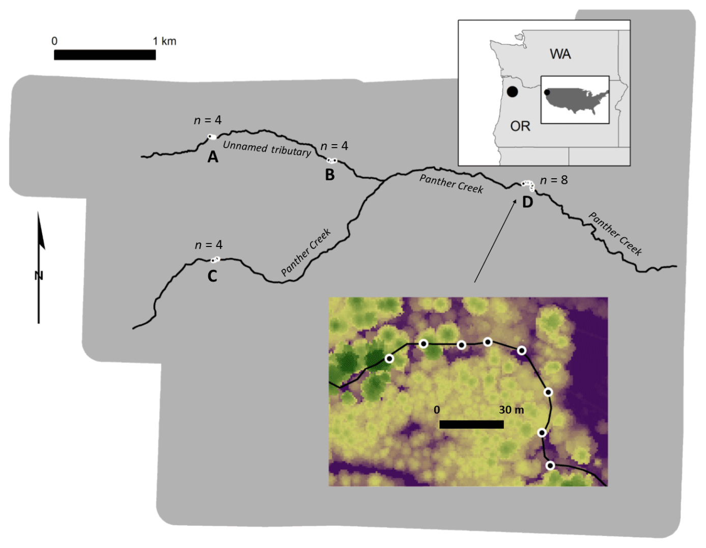
Figure 1Study area in northwestern Oregon (USA). The grey polygon is the extent of the 2015 lidar acquisition. The black circles surrounded by white circles represent the 19 point locations. The letters A–D denote the four transects. The inset shows transect D and the background raster in the inset is the lidar-derived canopy height model with green representing tall trees and purple representing the lowest heights. The direction of flow is from west to east.
1.3 Point cloud approaches
Because lidar point clouds are typically represented in a three-dimensional Cartesian coordinate system, it is possible to model the sun's position in relation to that three-dimensional space. The number of lidar returns that are reflected from a defined volume between the direction of the sun and the ground can then be calculated. These methods are computationally intensive, but have shown promise for providing the most direct measure of understory light availability. Lee et al. (2008) calculated the number of points within a conical field of view directed at the sun's location and created a model to relate this to ceptometer measurements of photosynthetically active understory solar radiation at specific times and locations in a pine forest in northern Florida, USA. This method is limited by its reliance on raw lidar point counts specific to the actual and relative point densities within their lidar acquisition. Raw point counts are affected by both changes in flight characteristics between missions and the patterns of flight line overlap within a mission. A different point cloud approach involves a linear tracing of the sun's rays along their path to the ground, and Martens et al. (2000) demonstrated how a ray-tracing algorithm could be used to characterize understory light conditions in a computer-simulated forest. Peng et al. (2014) combined a lidar-based ray tracing algorithm with field-collected canopy base heights to produce an estimate of understory solar insolation based on the Beer–Lambert law that compared well to field-collected pyranometer data but is limited in practical application because of its reliance on field-measured data in its model. Musselman et al. (2013) used a ray-tracing algorithm to produce highly detailed estimates of direct beam solar transmittance in 5-minute increments by voxelizing the lidar data and summing the number of voxels that a ray intercepted between the point of origin and the sun. The algorithm relied on site-specific pyranometer measurements to calibrate and adjust the beam transmittance, and therefore we were restricted from testing this method in this study.
Our objectives were to test the accuracy and precision of established methods of quantifying solar insolation from aerial lidar within areas of narrow, heavily forested streams. We utilized two raster approaches and one lidar point reprojection approach, three methodologies that had not been previously applied and tested using high-quality field data collected in heavily forested streams. We evaluated the three methodologies using simple linear regressions that compared lidar-derived metrics to field-based pyranometer measurements of solar insolation and hemispherical photograph-based measures of shade in western Oregon, USA. Further, we sought to apply this method to quantify solar insolation throughout a small headwater stream network.
2.1 Study site
All field locations were located within the wetted channel of Panther Creek and a tributary (Fig. 1) in narrow streams (1–6 m in width) located in the east side of the Coast Range of Oregon, USA, within a larger research area in which lidar has been used to quantify forest canopy structure (Flewelling and McFadden, 2011). All field sites were within a mature Douglas fir (Pseudotsuga menziesii) forest, with other dominant trees including red alder (Alnus rubra), western red-cedar (Thuja plicata), and western hemlock (Tsuga heterophylla). The elevation profile and description of the stream can be found in Richardson and Moskal (2014). The center of the channel was manually digitized as a polyline in ArcGIS using a combination of aerial imagery and the vendor-provided lidar DEM.
Four transects were installed in late June 2015 using a Leica Builder Total Station and georeferenced using a Javad Maxor GPS unit. The locations of the transects can be seen in Fig. 1, with the 19 point locations used for capturing field data denoted by black dots surrounded by white circles (A contains 3 points, B and C contain 4 points, and D contains 8 points). Transect locations were chosen manually in order to maximize variability in forest shade while allowing for safe access by the field crew. Each point location was located within the stream channel and marked by driving rebar into the substrate until only 1 m was exposed above the water surface. Point locations were approximately 15 m apart within a transect in order to allow data from multiple point locations to be collected by a single datalogger.
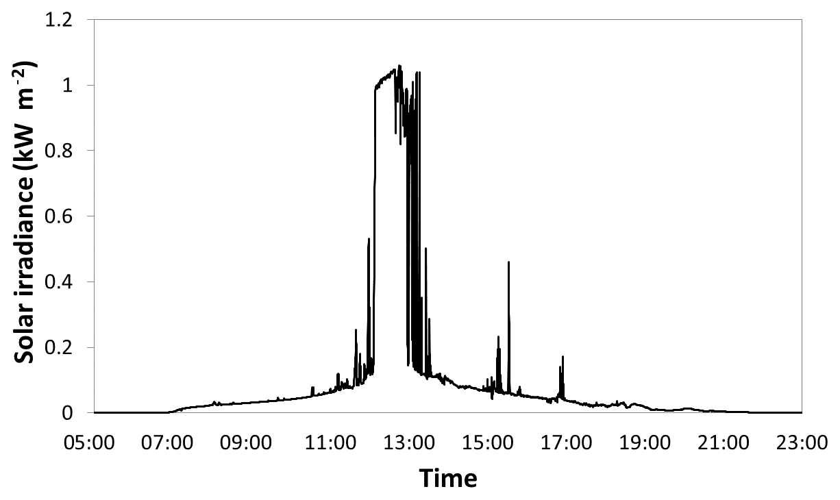
Two datasets were collected at each point location during the last 2 weeks of June in 2015. A hemispherical photograph was collected using a Nikon CoolPix 4500 digital camera leveled on a tripod 1 m above the ground under uniform sky conditions (Fig. 2) utilizing a method to find the optimum light exposure (Zhang et al., 2005). Each hemispherical photograph was analyzed using the Gap Light Analyzer (GLA) program (Frazer et al., 1999) in order to produce estimates of percent transmittance for diffuse and direct sunlight. An Apogee Instruments SP-110 self-powered silicon-cell pyranometer, leveled and mounted to the rebar pole at 1 m height (Fig. 3), was used to collect a full day's solar output at each point location using the datalogger. The raw voltage values collected by the datalogger were calibrated to solar irradiance using the closest publicly available meteorological data. All pyranometer datasets were collected on cloudless days, except for transect A, and pyranometer data from transect A were not used in this study. The calibrated pyranometer data from a point location from transect D are shown in Fig. 4. Note that the silicon-cell photodiodes, such as the SP-110 can, produce erroneous readings under conifer canopies. A black body thermopile pyranometer would have been more appropriate for this study but was not available to the authors.
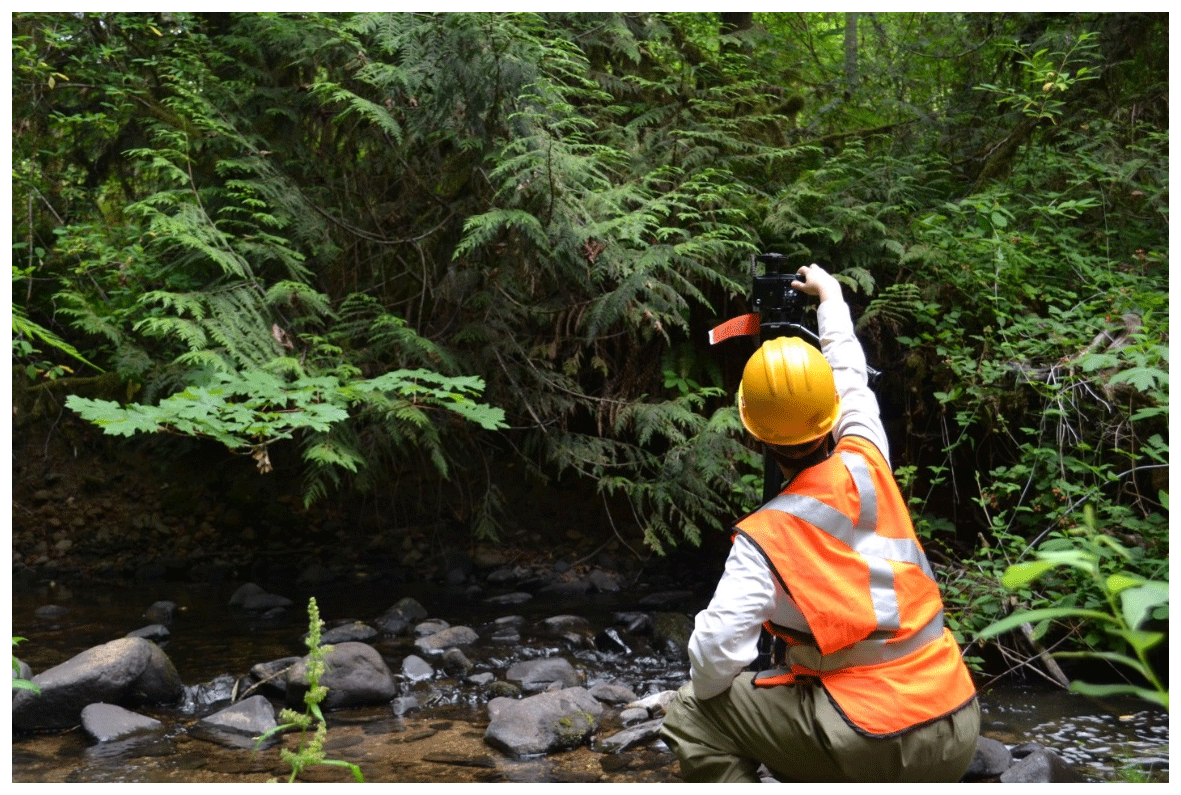
Figure 2Example of hemispherical photograph acquisition at a plot location in transect D.
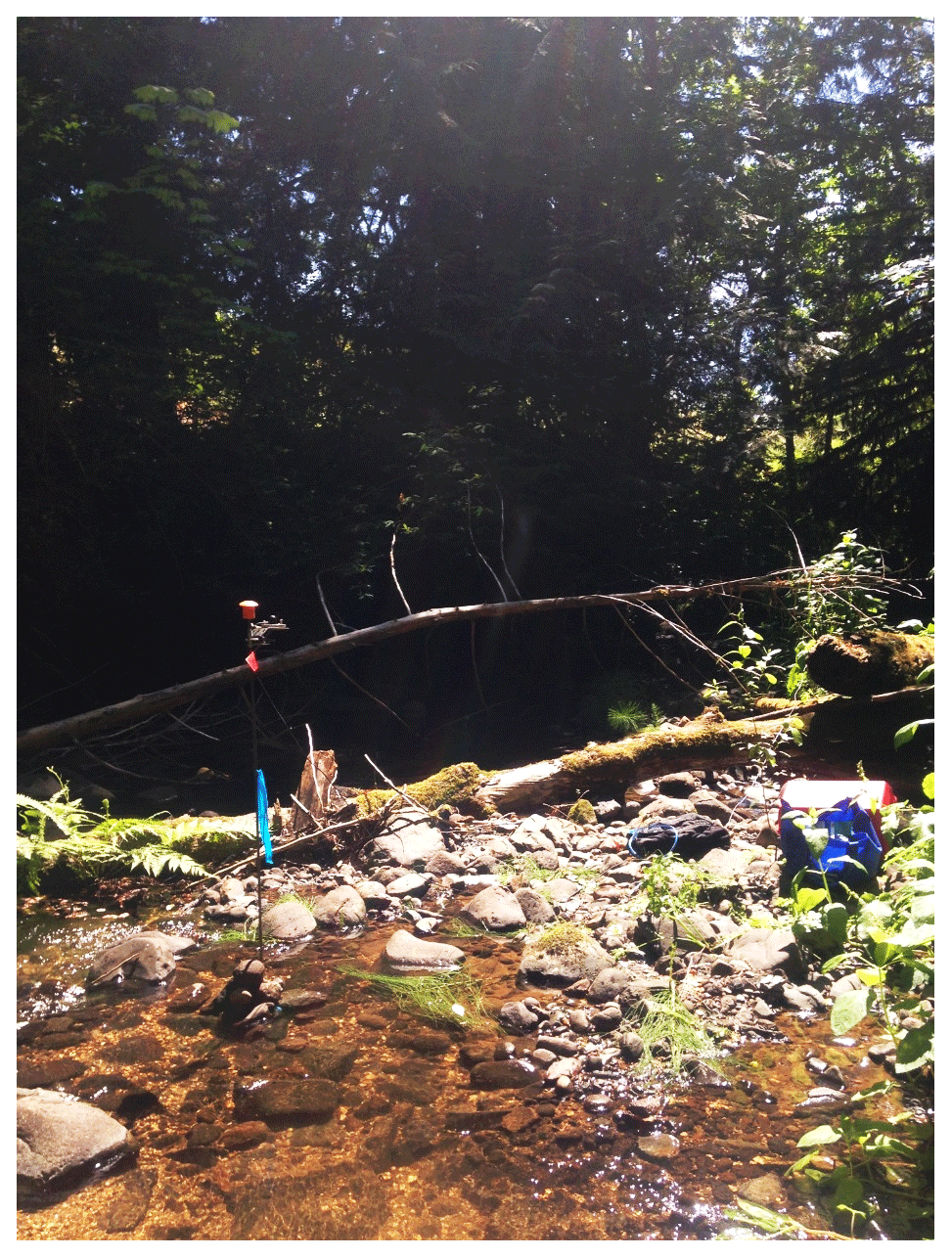
Figure 3Example of pyranometer installation at transect D (note that pyranometer is mounted on south side of pole at a height of 1 m).
2.2 Lidar data and analysis
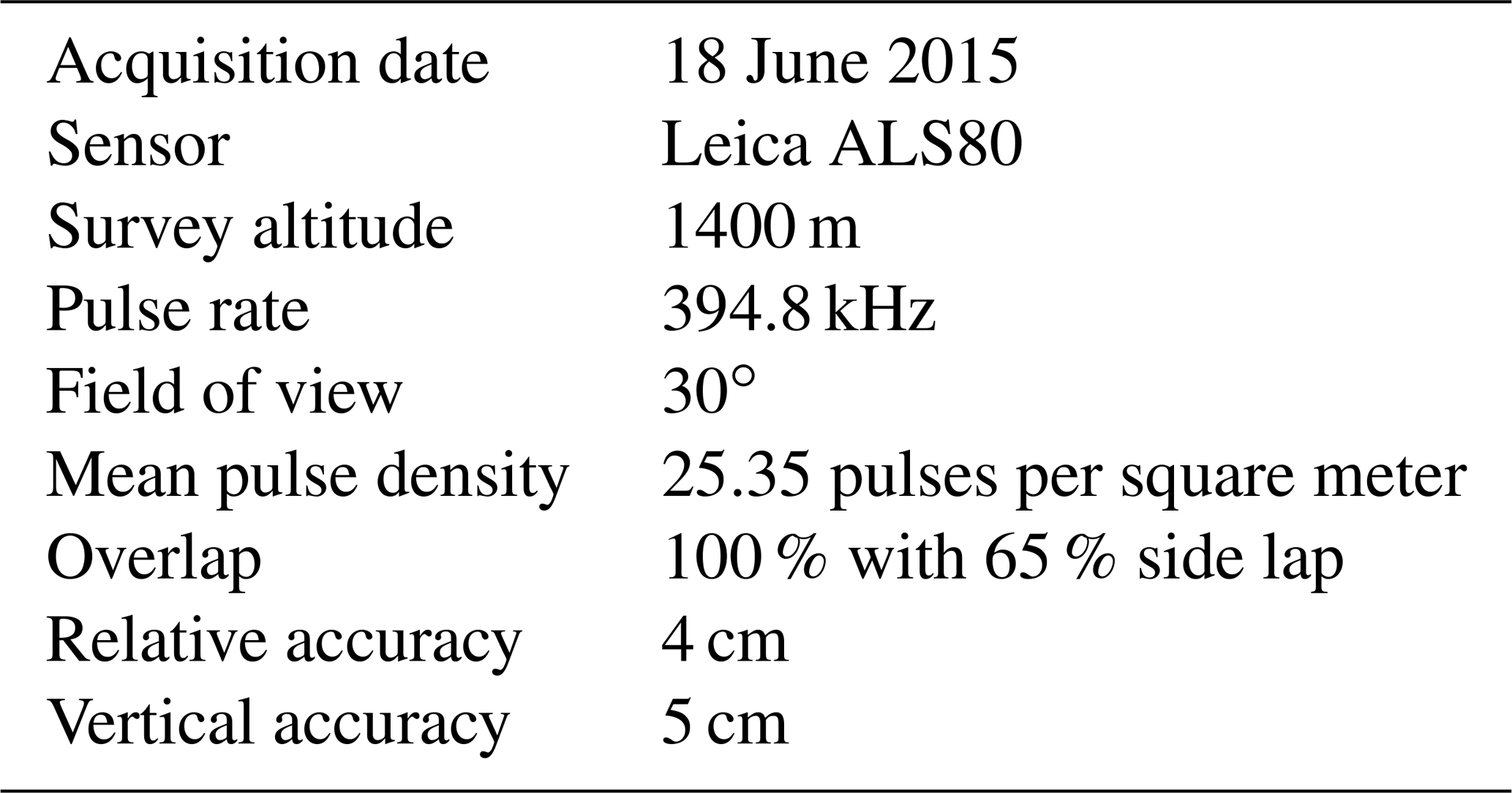
Airborne discrete-return lidar was acquired in June of 2015 according to the specifications described in Table 1. The vendor provided processed discrete lidar point returns as well as a lidar DEM and highest hit model at a pixel resolution of 1 m. The highest hit model was subtracted from the DEM to create a canopy height model (CHM) describing the vegetation height normalized to the ground surface. In addition, FUSION (McGaughey, 2009) was used to subtract the elevations of the raw lidar points from the ground elevation in the DEM to produce a normalized point cloud dataset (NPCD). Note that the perspective of the lidar analyses is in reference to ground height while the field data were collected at 1 m above the ground. While this is a small difference, it could be a source of error in comparisons, especially at low solar angles.
LPI was computed as follows:
LPI was computed in ArcGIS using a circular buffer with radius 10 m around each field point location mirroring the radius used in Richardson et al. (2009). LPI was also computed using a shifted square buffer modified from the method of Bode et al. (2014) where the buffer side length (s) was calculated based on the following:
where h is equal to the modal tree height across all our plots (34 m), and θ is equal to the maximum lidar scan angle subtracted from 90∘ (75∘), resulting in a buffer side length of 9.12 m. The square buffer was shifted south to account for the seasonal solar angle in the Northern Hemisphere according to the following:
where σ is equivalent to the solar angle at noon on the date of interest. A solar angle of 68∘ was used in this study, resulting in a southern shift of 3.42 m. The buffer tool, zonal statistics tool, and move command were used to achieve the shift in ArcGIS. We also computed topographically influenced solar radiation using the lidar DEM and the solar radiation function in ArcGIS, but found that there was no significant difference across the plot locations and thus did not use these results in subsequent analysis.
Synthetic hemiphotos were created in MATLAB using the method of Moeser et al. (2014) and analyzed for diffuse and direct light transmittance in GLA. All statistical analyses were performed in R (version 3.4).
Longitudinal profiles of stream shading were created in ArcGIS in 1 m increments based on the intersections of the stream polyline center line with the raster output of modeled solar insolation.
3.1 Comparison between pyranometers and hemispherical photographs
Figure 5 shows the correlation between field-collected pyranometer data and processed hemispherical photographs, with data from transect A removed. These data are highly correlated (r2=0.87), but these data are also not equally distributed across a range of solar insolation. Many more plot locations were at low levels of solar insolation than in areas of relatively low shade. This is very typical of the heavily forested streams in northwestern North America. Note that none of our plot locations contained transmittance greater than 40 %.
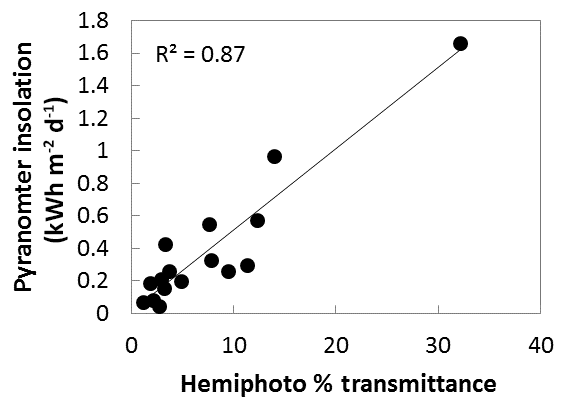
Figure 5Comparison between pyranometer-measured solar insolation and daily diffuse and direct radiation canopy transmittance calculated from hemispherical photographs.
3.2 Linear regressions
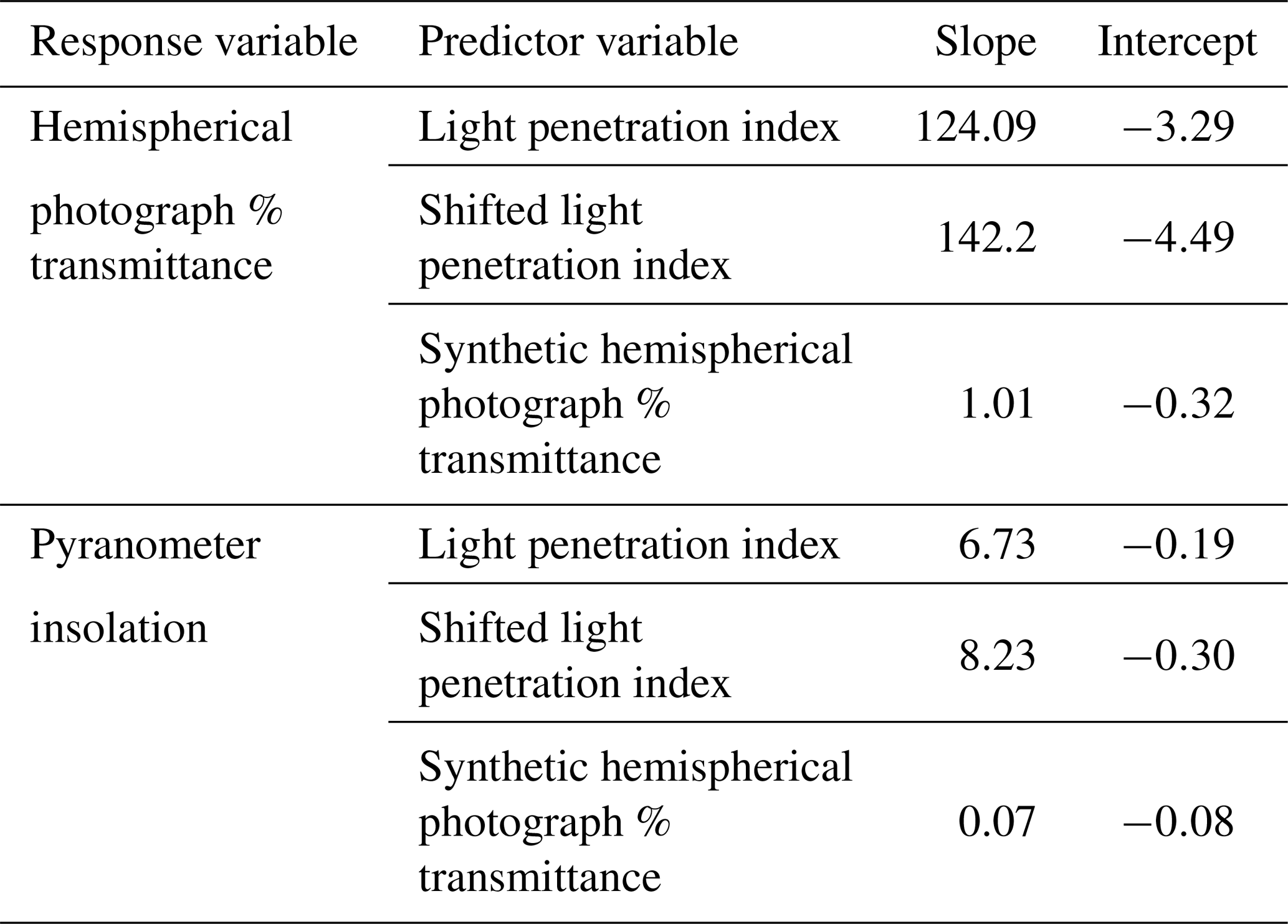
Pyranometer-based solar insolation and hemispherical photograph percent diffuse and direct radiation transmittance calculated at all point locations except transect A were compared to three lidar predictors using simple linear regression. These results are shown in Fig. 6. The LPI calculated using a 10 m circle centered on the point location explained about 55 % of the variability in both response variables, but the prediction accuracy improved when LPI was calculated using the shifted square buffer. Shifted LPI explained 74 % of the variability in solar insolation and 64 % of the variability in percent transmittance. Synthetic hemispherical photographs explained 77 % of the variability in solar insolation and 60 % of the variability in percent transmittance. Figure 6 shows comparisons between transects B and D to make interpretation easier, but Table 2 shows the results of linear regressions between predicted variables and hemispherical photograph transmittance for all plot locations resulting in small reductions in the amount of variability explained. Table 3 gives parameters of slope and intercept resulting from the simple linear regression.
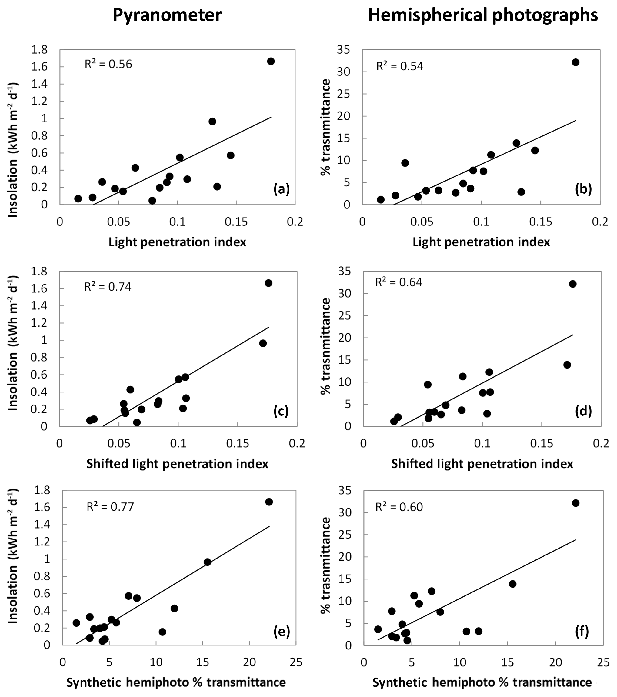
Figure 6Simple linear regressions between lidar predictor variables and field-measured pyranometer solar insolation (a, c, e) and hemispherical photograph percentage transmittance (b, d, f) omitting data from transect A.
Table 2Coefficients of determination for the simple linear regression between predictor variables and hemispherical photograph transmittance using three additional point locations from transect A.
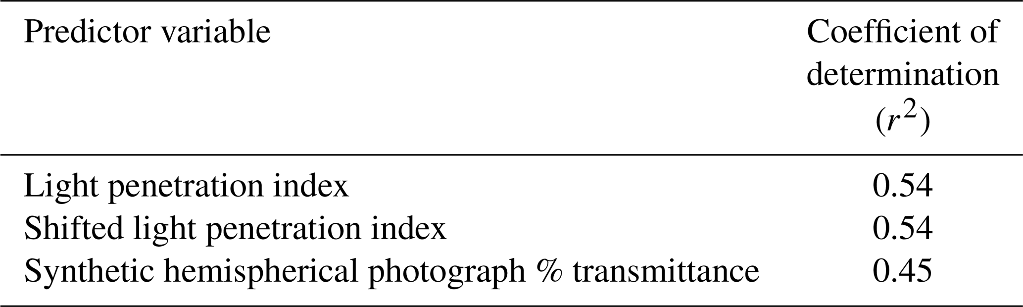
Table 3Parameters from simple linear regressions. Note that all regressions are significant (p<0.05). Data from transect A are excluded.
While both the raster-based shifted LPI approach and the lidar point reprojection synthetic hemispherical photograph approach explained more than 60 % of the variability in the field data, the limited range of solar insolation conditions at the point locations in our study may limit some of the conclusions that can be drawn. Excluding transect A, 14 of the 16 point locations received less than 0.8 kWh m−2 d−1, leading the other two point locations to exert a large degree of leverage on the results. Note that these two point locations received less than 35 % of the maximum solar insolation. The three points in transect A all received less than 0.8 kWh m−2 d−1 and their inclusion in Table 2 did not improve coefficients of determination, suggesting that all methods are not as effective at predicting field-measured values in areas of high canopy cover. The constraints of the study design requiring point locations to be located in the stream made it impossible to achieve a greater range in solar insolation. It is reasonable to expect that including more point locations receiving larger amounts of insolation would have led to improved accuracy and greater coefficients of determination, as previous studies have shown that accuracy increases as canopy cover decreases (Moeser et al., 2014; Musselman et al., 2013; Richardson and Moskal, 2014).
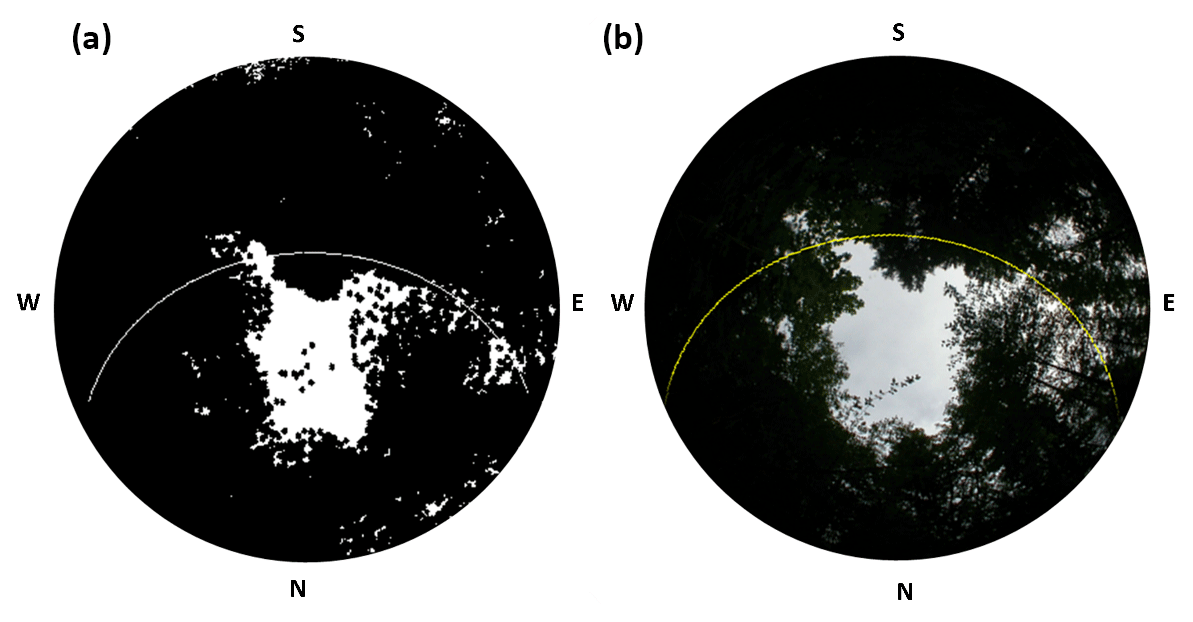
Figure 7Sun path superimposed on a synthetic hemispherical photograph (a) and a field-acquired hemispherical photograph (b) at a point location in Transect D. The letters represent the four cardinal directions.
One explanation of the decrease in variability at high canopy cover in regressions E and F shown in figure is demonstrated in Fig. 7. Here, a synthetic hemispherical photograph from transect D is compared to a field-captured hemispherical photograph with the GLA modeled sun path superimposed. This sun path is critical for determining the quantity of direct light, but very small differences in the center location of the two images can produce large differences in the modeled direct light. The sun path passes through a modeled canopy gap near solar noon on the synthetic hemispherical photograph, while it intersects only canopy and misses the gap on the field-collected hemispherical photograph. Very small registration errors can cause differences in transmittance at low light levels, and we suggest that these errors are likely to cause the errors observed in the regressions. The daily pyranometer output for the same point location is shown in Fig. 8 to further aid comparison. The pyranometer is only briefly exposed to full sunlight, highlighting the contribution of small gaps in the canopy.
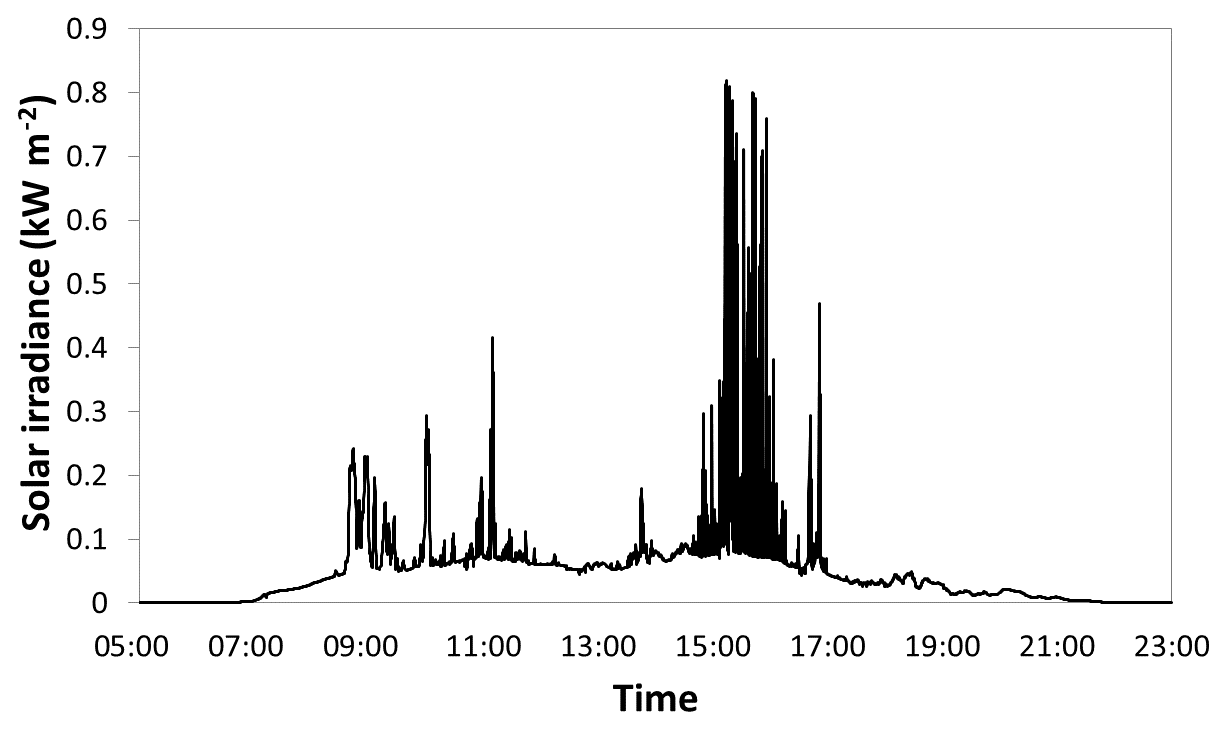

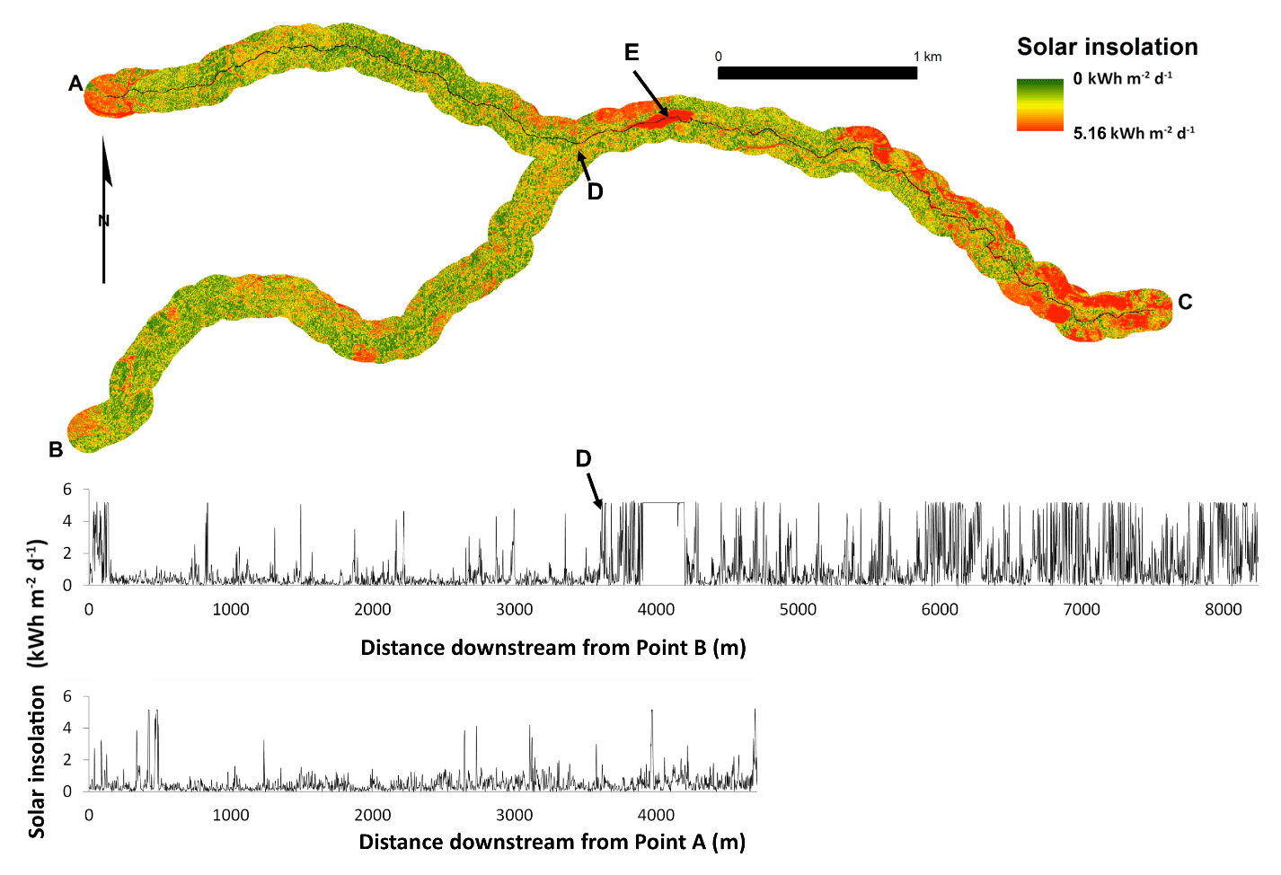
Figure 10Map of model-derived solar insolation for Panther Creek (top) and graph of model-derived solar insolation for reach A–C (middle) and reach B–D (bottom). Point E is a dammed reservoir. Note the direction of flow is toward point C.
Understory vegetation is another likely cause of observed errors, as airborne lidar is inherently limited in its ability to fully sample multi-layered canopies (Richardson and Moskal, 2011). We noticed several points with differences between lidar predictors and field data that contained understory vegetation in close proximity to the field instruments. The ideal scenario would be for the lidar scan angles to precisely match the range of potential solar angles at each plot location, but this is currently impractical, leading to an incomplete sample of the canopy light environment which contributes to the observed errors.
3.3 Modeled solar insolation
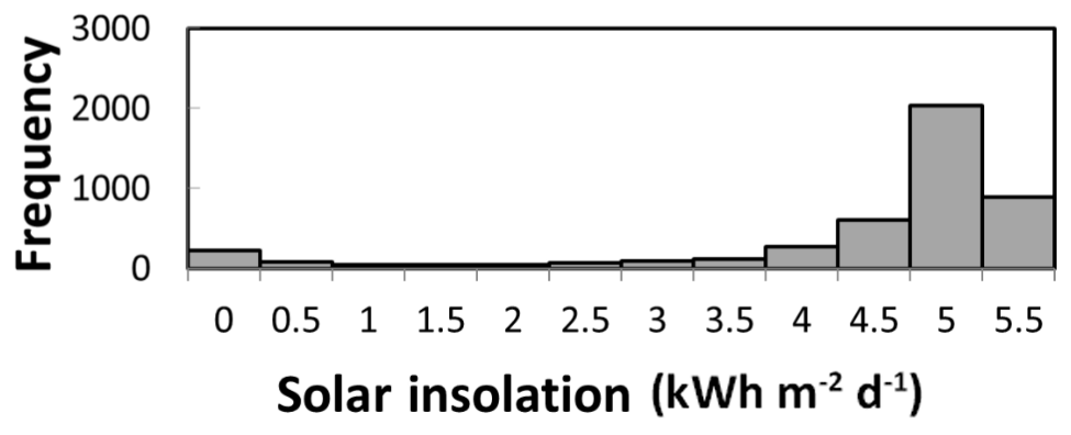
The correlations between lidar predictors and field data were strongest in Fig. 6c and e, and these lidar predictors are both appropriate to use as the basis for estimating solar insolation across the study area. Implementation of shifted LPI was the simplest and least time-intensive method, and we chose to model solar radiation by multiplying shifted LPI by the maximum above-canopy solar insolation for 20 June 2015 and then computing a non-intercept linear regression (Fig. 9). Removing the intercept from the model lowered the coefficient of determination but provided a model that did not estimate negative values of solar insolation. Figure 10 shows the model applied across the study area. The graphs show the pattern of solar insolation across the two reaches in the study, highlighting the utility of these methods for predicting solar insolation in heavily forested streams across wide spatial extents. Figure 11 shows the relative frequency of binned solar insolation values, highlighting the dominance of heavily shaded areas (note that a dammed reservoir, point D on the map, contributes the majority of the points in full sun).
The relatively unbiased results shown in Fig. 9 show that field calibration is not required to produce accurate estimates of solar insolation. However, information is still needed on local above-canopy meteorological conditions, which can either be modeled from known solar outputs or collected from a nearby meteorological station. Little bias was observed in comparisons between synthetic hemispherical photograph transmittance and field-based hemispherical photograph transmittance (Table 3). Therefore, both approaches tested in this study should not require field calibration.
We tested two approaches for estimating solar insolation from airborne lidar using field data collected in a heavily forested narrow stream, showing that an LPI-based raster approach and a synthetic hemispherical photograph approach can predict solar insolation and light transmittance. These results should be interpreted with the caveat that our point locations contained few areas with high insolation. We showed that the LPI-based model can be applied across the landscape, and we demonstrated that no field-based calibration was necessary to produce unbiased prediction of solar insolation.
This study lays the groundwork for additional research on remote sensing methods for quantifying light conditions in riparian areas over heavily forested streams. One method that we were unable to test is ray-tracing, and future research should continue to develop this approach. Second, research should focus on exploring the limit of matching ground-based measurements to lidar-predicted solar insolation. Lastly, the limitation of aerial lidar to quantify understory light conditions in multi-layered canopies should be explored in more detail to better understand when and if airborne sensors are inappropriate for these particular applications. In these circumstances, other sensors such as terrestrial lidar or ground-based digital photographs utilizing structure from motion may provide additional useful information.
The GPS data, pyranometer data, processed hemispherical photograph data, spreadsheets used for data analysis, and access to the lidar data can be found at https://doi.org/10.17632/vwmxw4hcj7.1 (Richardson, 2018).
JJR, LLM, and CET designed the study design. LLM and CET secured funding. JJR performed the data analysis and prepared a draft of the manuscript. CET provided review and editing of the manuscript.
The authors declare that they have no conflict of interest.
We are grateful to Dave Moeser for sharing his MATLAB code for creating synthetic hemispherical photographs and to Keith Musselman for advising on the applicability of ray-tracing methods. Guang Zheng also assisted with research into ray-tracing methods. Caileigh Shoot and Natalie Gray coordinated field data collection. This work was supported by the Precision Forestry Cooperative, the Bureau of Land Management, and the US Geological Survey. Any use of trade, product or firm names is for descriptive purposes only and does not imply endorsement by the US government.
This paper was edited by Martijn Westhoff and reviewed by Collin Bode, Caleb Buahin, and one anonymous referee.
Alexander, C., Moeslund, J. E., Bocher, P. K., Arge, L., and Svenning, J. C.: Airborne laser scanner (LiDAR) proxies for understory light conditions, Remote Sens. Environ., 134, 152–161, https://doi.org/10.1016/j.rse.2013.02.028, 2013.
Ameztegui, A., Coll, L., Benavides, R., Valladares, F., and Paquette, A.: Understory light predictions in mixed conifer mountain forests: Role of aspect-induced variation in crown geometry and openness, Forest Ecol. Manage., 276, 52–61, https://doi.org/10.1016/j.foreco.2012.03.021, 2012.
Asrar, G., Myneni, R. B., and Choudhury, B. J.: Spatial heterogeneity in vegetation canopies and remote sensing of absorbed photosynthetically active radiation: A modeling study, Remote Sens. Environ., 41, 85–103, https://doi.org/10.1016/0034-4257(92)90070-Z, 1992.
Bode, C. A., Limm, M. P., Power, M. E., and Finlay, J. C.: Subcanopy Solar Radiation model: Predicting solar radiation across a heavily vegetated landscape using LiDAR and GIS solar radiation models, Remote Sens. Environ., 154, 387–397, https://doi.org/10.1016/j.rse.2014.01.028, 2014.
Breshears, D. D., Rich, P. M., Barnes, F. J., and Campbell, K.: Overstory-imposed heterogeneity in solar radiation and soil moisture in a semiarid woodland, Ecol. Appl., 7, 1201–1215, https://doi.org/10.2307/2641208, 1997.
Field, C. B., Randerson, J. T., and Malmström, C. M.: Global net primary production: Combining ecology and remote sensing, Remote Sens. Environ., 51, 74–88, https://doi.org/10.1016/0034-4257(94)00066-V, 1995.
Flewelling, J. W. and McFadden, G.: LiDAR data and cooperative research at Panther Creek, Oregon, in: SilviLaser, 16–20 October 2011, Hobart, Australia, 2011.
Forney, W. M., Soulard, C. E., and Chickadel, C. C.: Salmonids, stream temperatures, and solar loading–modeling the shade provided to the Klamath River by vegetation and geomorphology, US Geological Survey Scientific Investigations Report 2013-5022, p. 25, available at: http://pubs.usgs.gov/sir/2013/5022/ (last access: July 2019), 2013.
Frazer, G. W., Canham, C. D., and Lertzman, K. P.: Gap Light Analyzer (GLA), Version 2.0, Simon Fraser University, Burnaby, British Columbia, 1999.
Hock, R.: Temperature index melt modelling in mountain areas, J. Hydrol., 282, 104–115, https://doi.org/10.1016/S0022-1694(03)00257-9, 2003.
Holtby, L. B.: Effects of logging on stream temperatures in Carnation Creek British Columbia, and associated impacts on the coho salmon (Oncorhynchus kisutch), Can. J. Fish. Aquat. Sci., 45, 502–515, https://doi.org/10.1139/f88-060, 1988.
Kerr, J. P., Thurtell, G. W., and Tanner, C. B.: An integrating pyranometer for climatological observer stations and mesoscale networks, J. Appl. Meteorol., 6, 688–694, https://doi.org/10.1175/1520-0450(1967)006<0688:AIPFCO>2.0.CO;2, 1967.
Lee, H., Slatton, K. C., Roth, B. E., and Cropper, W. P.: Prediction of forest canopy light interception using three-dimensional airborne LiDAR data, Int. J. Remote Sens., 30, 189–207, https://doi.org/10.1080/01431160802261171, 2008.
Leinenbach, P., McFadden, G., and Torgersen, C. E.: Effects of riparian management strategies on stream temperature, Interagency Coordinating Subgroup, Seattle, WA, 22 pp., 2013.
Martens, S. N., Breshears, D. D., and Meyer, C. W.: Spatial distributions of understory light along the grassland/forest continuum: effects of cover, height, and spatial pattern of tree canopies, Ecol. Model., 126, 79–93, https://doi.org/10.1016/S0304-3800(99)00188-X, 2000.
McGaughey, R. J.: FUSION/LDV: software for LIDAR data analysis and visualization, 2.51 Edn., United States Department of Agriculture, Forest Service, Pacific Northwest Research Station, Seattle, WA, 2009.
Moeser, D., Roubinek, J., Schleppi, P., Morsdorf, F., and Jonas, T.: Canopy closure, LAI and radiation transfer from airborne LiDAR synthetic images, Agr. Forest Meteorol., 197, 158–168, https://doi.org/10.1016/j.agrformet.2014.06.008, 2014.
Moore, R. D., Spittlehouse, D. L., and Story, A.: Riparian microclimate and stream temperature response to forest harvesting: a review, JAWRA J. Am. Water Resour. Assoc., 41, 813–834, 2005a.
Moore, R. D., Sutherland, P., Gomi, T., and Dhakal, A.: Thermal regime of a headwater stream within a clear-cut, coastal British Columbia, Canada, Hydrol. Process., 19, 2591–2608, https://doi.org/10.1002/hyp.5733, 2005b.
Musselman, K. N., Margulis, S. A., and Molotch, N. P.: Estimation of solar direct beam transmittance of conifer canopies from airborne LiDAR, Remote Sens. Environ., 136, 402–415, https://doi.org/10.1016/j.rse.2013.05.021, 2013.
Musselman, K. N., Pomeroy, J. W., and Link, T. E.: Variability in shortwave irradiance caused by forest gaps: measurements, modelling, and implications for snow energetics, Agr. Forest Meteorol., 207, 69–82, https://doi.org/10.1016/j.agrformet.2015.03.014, 2015.
Nicotra, A. B., Chazdon, R. L., and Iriarte, S. V. B.: Spatial heterogeneity of light and woody seedling regneration in tropical wet forests, Ecology, 80, 1908–1926, https://doi.org/10.1890/0012-9658(1999)080[1908:SHOLAW]2.0.CO;2, 1999.
Ni-Meister, W., Strahler, A. H., Woodcock, C. E., Schaaf, C. B., Jupp, D. L. B., Yao, T., Zhao, F., and Yang, X.: Modeling the hemispherical scanning, below-canopy lidar and vegetation structure characteristics with a geometric-optical and radiative-transfer model, Can. J. Remote Sens., 34, S385–S397, https://doi.org/10.5589/m08-047, 2008.
Peng, S. Z., Zhao, C. Y., and Xu, Z. L.: Modeling spatiotemporal patterns of understory light intensity using airborne laser scanner (LiDAR), ISPRS J. Photogramm. Remote Sens., 97, 195–203, https://doi.org/10.1016/j.isprsjprs.2014.09.003, 2014.
Rich, P., Dubayah, R., Hetrick, W., and Saving, S.: Using viewshed models to calculate intercepted solar radiation: applications in ecology, American Society for Photogrammetry and Remote Sensing Technical Papers, American Society of Photogrammetry and Remote Sensing, Reno, NV, 524–529, 1994.
Richardson, J. J.: Lidar-based modelling approaches for estimating solar insolation in heavily forested streams, Mendeley Data, https://doi.org/10.17632/vwmxw4hcj7.1, 2018.
Richardson, J. J. and Moskal, L. M.: Strengths and limitations of assessing forest density and spatial configuration with aerial LiDAR, Remote Sens. Environ., 115, 2640–2651, https://doi.org/10.1016/j.rse.2011.05.020, 2011.
Richardson, J. J. and Moskal, L. M.: Assessing the utility of green LiDAR for characterizing bathymetry of heavily forested narrow streams, Remote Sens. Lett., 5, 352–357, https://doi.org/10.1080/2150704X.2014.902545, 2014.
Richardson, J. J., Moskal, L. M., and Kim, S.-H.: Modeling approaches to estimate effective leaf area index from aerial discrete-return LIDAR, Agr. Forest Meteorol., 149, 1152–1160, https://doi.org/10.1016/j.agrformet.2009.02.007, 2009.
Torgersen, C. E., Hockman-Wert, D. P., Bateman, D. S., Leer, D. W., and Gresswell, R. E.: Longitudinal patterns of fish assemblages, aquatic habitat, and water temperature in the Lower Crooked River, Oregon, United States Geological Survey, Reston, VA, 37 pp., https://doi.org/10.3133/ofr20071125, 2007.
Torgersen, C. E., Ebersole, J. L., and Keenan, D. M.: Primer for identifying cold-water refuges to protect and restore thermal diversity in riverine landscapes, Seattle, WA, Document number: EPA 910-C-12-001, US Environmental Protection Agency, Seattle, WA, 91 pp., 2012.
Zhang, Y. Q., Chen, J. M., and Miller, J. R.: Determining digital hemispherical photograph exposure for leaf area index estimation, Agr. Forest Meteorol., 133, 166–181, 2005.