the Creative Commons Attribution 4.0 License.
the Creative Commons Attribution 4.0 License.
 | 10 Jul 2019
Bayesian performance evaluation of evapotranspiration models based on eddy covariance systems in an arid region
Guoxiao Wei
Xiaoying Zhang
Ming Ye
Ning Yue
Fei Kan
Evapotranspiration (ET) is a major component of the land surface process involved in energy fluxes and energy balance, especially in the hydrological cycle of agricultural ecosystems. While many models have been developed as powerful tools to simulate ET, there is no agreement on which model best describes the loss of water to the atmosphere. This study focuses on two aspects, evaluating the performance of four widely used ET models and identifying parameters, and the physical mechanisms that have significant impacts on the model performance. The four tested models are the Shuttleworth–Wallace (SW) model, Penman–Monteith (PM) model, Priestley–Taylor and Flint–Childs (PT–FC) model, and advection–aridity (AA) model. By incorporating the mathematically rigorous thermodynamic integration algorithm, the Bayesian model evidence (BME) approach is adopted to select the optimal model with half-hourly ET observations obtained at a spring maize field in an arid region. Our results reveal that the SW model has the best performance, and the extinction coefficient is not merely partitioning the total available energy into the canopy and surface but also including the energy imbalance correction. The extinction coefficient is well constrained in the SW model and poorly constrained in the PM model but not considered in PT–FC and AA models. This is one of the main reasons that the SW model outperforms the other models. Meanwhile, the good fitting of SW model to observations can counterbalance its higher complexity. In addition, the detailed analysis of the discrepancies between observations and model simulations during the crop growth season indicate that explicit treatment of energy imbalance and energy interaction will be the primary way of further improving ET model performance.


Surface energy fluxes are an important component of Earth's global energy budget and a primary determinant of surface climate. Evapotranspiration (ET), as a major energy flux process for energy balance, accounts for about 60 %–65 % of the average precipitation over the surface of the Earth (Brutsaert, 2005). In agricultural ecosystems, more than 90 % of the total water losses are due to ET (Morison et al., 2008). Therefore, robust ET estimation is crucial to a wide range of problems in hydrology, ecology, and global climate change (Xu and Singh, 1998). In practice, mtuch of our understanding of how land surface processes and vegetation affect weather and climate is based on numerical modeling of surface energy fluxes and the atmospherically coupled hydrological cycle (Bonan, 2008). Several models are commonly used in agricultural systems to evaluate ET. The Penman–Monteith (PM) and Shuttleworth–Wallace (SW) models are physically sound and rigorous (Zhu et al., 2013) and thus widely used to simulate ET for seasonally varied vegetation. The models consider the relationships between net radiation, all kinds of heat flux (such as latent heat, sensible heat, and heat from soil and canopy), and surface temperature. The Priestley–Taylor and Flint–Childs (PT–FC) model (based on radiation) and the advection–aridity (AA) model (based on meteorological variables) have also been widely used because they only require a small number of ground-based measurements to set up the models (Ershadi et al., 2014).
Comparing the performance of the competing ET models and evaluating and understanding the discrepancies between simulations of the models and corresponding observed surface–atmosphere water flux remain challenging problems (Legates and McCabe, 1999). Both non-Bayesian analysis (Szilagyi and Jozsa, 2008; Vinukollu et al., 2011; Li et al., 2013; Ershadi et al., 2015) and Bayesian analysis have been used to evaluate the performance of ET models (Zhu et al., 2014; Chen et al., 2015; Liu et al., 2016; Zhang et al., 2017; Elshall et al., 2018; Samani et al., 2018;). Li et al. (2013) compared the ET simulations of the PM, SW and adjusted SW models under film-mulching conditions of maize growth in an arid region of China. They found that the half-hourly ET was overestimated by 17 % in the SW model. In contrast, the PM and adjusted SW models underestimated the daily ET by 6 % and 2 %, respectively. Therefore, the performances of PM and adjusted SW models are better than those of the SW model in their case study. Ershadi et al. (2014) evaluated the surface energy balance system (SEBS), PM, PT–JPL (JPL is the Priestley–Taylor Propulsion Laboratory Model; a modified Priestley–Taylor model), and AA models. Based on the average value of model efficiency (EF) and RMSE, the model ranking from worst to best was AA, PM, SEBS, and PT–JPL. Ershadi et al. (2015) also compared the response of the models to different formulations of aerodynamic and surface resistances with global FLUXNET data. Their results showed considerable variability in model performance among and within biome types. Currently, ET model selection and comparison have been still conducted using traditional error metrics. It is known that error metrics are not adequate for providing a reasonable result of model ranking for disregarding model complexity (Marshall et al., 2005; Samani et al., 2018). The focus of this study is to use a Bayesian approach to evaluate the performance of the PM, SW, PT–FC, and AA models, which is a novelty contribution of this study. In ET models, the land surface energy system is governed by presumably infinitely dimensional physics. However, considering the ET models to be finitely dimensional can be more precise by covering all relevant relations. Therefore, employing consistent criteria for model selection might be justified when the aim is to better understand the processes involved (Höge et al., 2018). When using consistent model selection, Bayesian model evidence (BME), also known as marginal likelihood, measures the average fit of model simulations to their corresponding observations over a model's prior parameter space. This feature enables BME to consider model complexity (in terms of the number of model parameters) for model performance evaluation. When comparing several alternative conceptual models, the model with the largest marginal likelihood is selected as the best model (Lartillot and Philippe, 2006). BME can thus be used for evaluating the model fit (over the parameter space) and for comparing alternative models. In previous studies, the Bayesian information criterion (BIC; Schwarz, 1978) and the Kashyap information criterion (KIC; Kashyap, 1982) have been used to approximate BME by using maximum likelihood theories to reduce the computational cost of evaluating BME (Ye et al., 2004). However, these approximations have theoretical and computational limitations (Ye et al., 2008; Xie et al., 2011; Schöniger et al., 2014), and a numerical evaluation (not a likelihood approximation) of BME is necessary, especially for complex models (Lartillot and Philippe, 2006). Lartillot and Philippe (2006) advocated the use of thermodynamic integration (TI) for estimating BME, also known as path sampling (Gelman and Meng, 1998; Neal, 2000), in order to avoid sampling solely in the prior or posterior parameter space. TI uses samples that are systematically generated from the prior to the posterior parameter space by conducting path sampling with several discrete power coefficient values (Liu et al., 2016). It is more numerically accurate than the generally used harmonic mean method (Xie et al., 2011).
Most applications of Bayesian methods have focused on the calibration of individual models, while the comparison of alternative models continues to be performed using traditional error metrics. More generally, Bayesian approaches to model calibration, comparison, and analysis have been used far less in the evaluation of ET models than in other areas of environmental science. In this study, the Bayesian approach is used to calibrate and evaluate the four ET models (PM, SW, PT–FC, and AA) based on an experiment over a spring maize field in an arid area of northwestern China from 3 June to 27 September 2014. The objectives of the study are as follows: (1) to calibrate ET model parameters using the DiffeRential Evolution Adaptive Metropolis (DREAM) algorithm (Vrugt et al., 2008, 2009), (2) to identify which parameters had a greater impact on the model performance and to explain why the selected optimal model performed best, (3) to evaluate the performance of the models using traditional error metrics and BME, and (4) to analyze discrepancies between model simulations and observation data in order to better understand model performance and identify ways to improve these models. We expect that the study will not only boost the development of model parameterization and model selection but also contribute to the improvement of the ET models.
2.1 Description of the study area
The experiment of maize growth was conducted at the Daman Superstation, located in Zhangye, Gansu province, northwestern China. Daman oasis is located in the middle Heihe River basin, which is the second largest inland river basin in the arid region of northwestern China. The midstream area of the Heihe River basin is characterized by oases with irrigated agriculture and is a region that consumes a large amount of water for both domestic and agricultural uses. The annual average precipitation and temperature are 125 mm and 7.2∘ (1960–2000), respectively. The annual accumulated temperature (>10∘) is 3234∘, and the annual average potential evaporation is about 2290 mm. The average annual duration of sunshine is 3106 h, with 148 frost-free days. The predominant soil type is silty-clay loam, and the depth of the frozen layer is about 143 mm. The study area is a typical irrigated agricultural region, and the major source of water is snowmelt from the Qilian Mountains. Maize and spring wheat are the principal crops grown in the region. Maize is generally sown in late April and harvested in mid-September and is planted with a row spacing of 40 cm and a plant spacing of 30 cm. The plant density is about 66 000 plants ha−1 in the study area.
2.2 Measurements and data processing
Our data were collected from the field observation systems of the Heihe Watershed Allied Telemetry Experimental Research (HiWATER) project as described in Li et al. (2013). The observation period was from DOY (day of the year) 154 to DOY 270 in 2014. An open-path eddy covariance (EC) system was installed in a maize field, with the sensors at a height of 4.5 m. Maize is the main crop in the study region and thus covers sufficient planting area to set the EC measurements. The EC data were logged at a frequency of 10 Hz and then processed with an average time interval of 30 min. Sensible and latent heat fluxes were computed by the EC approach of Baldocchi (2003). Flux data measured by EC were controlled by traditional methods, including three-dimensional rotation (Aubinet et al., 2000); Webb–Penman–Leuning (WPL) density fluctuation correction (Webb et al., 1980); frequency response correction (Xu et al., 2014); and spurious data removal caused by rainfall, water condensation, and system failure. About 85 % of the energy balance closure was observed in the EC data (Liu et al., 2011).
Standard hydro-meteorological variables, including rainfall, air temperature, wind speed, and wind direction, were continuously measured at the heights of 3, 5, 10, 15, 20, 30, and 40 m above the ground. Soil temperature and moisture were measured at heights of 2, 4, 10, 20, 40, 80, 120, and 160 cm. Photosynthetically active radiation was measured at a height of 12 m. Net radiation, including downward, upward, and longwave radiation, was measured by a four-component net radiometer. An infrared thermometer was installed at a height of 12 m. The leaf area index (LAI) was measured approximately every 10 d during the growing season.
2.3 Model description
In this section, we summarize the mathematical definitions forming the basis of each of the four models. Appendix A contains a summary of the names and physical meanings of the model parameters.
2.3.1 Penman–Monteith (PM) model
The PM model can be formulated in the following way (Monteith, 1965):
where , and A is defined as .
In the present study, ga is parameterized in the way suggested by Leuning et al. (2008), and gs is defined as
where 1−τ and τ are the fractions of the total available energy absorbed by the canopy and by the soil, τ=exp (KaLAI), and gi and are defined in Eqs. (3) and (4), respectively (Monteith, 1965),
where f(θ) represents water stress and is expressed as
and θa is set as θa=0.75 θb. Aerodynamic conductance ga is calculated as
where the quantities d, z0 m, and z0 v are calculated using , z0 m=0.123 h, and (Allen et al., 1998).
2.3.2 Shuttleworth–Wallace (SW) model
The SW model comprises a one-dimensional model of plant transpiration and a one-dimensional model of soil evaporation. The two terms are calculated by the following equations:
where the available energy input above the soil surface is defined as .
Rns can be calculated using the Beer's law relationship:
The coefficients Cs and Cc are obtained as follows:
where
Soil surface resistance is expressed as
In this study, we consider the reciprocal of bulk stomatal resistance, known as canopy conductance. The calculation of is the same as in the PM model. The two aerodynamic resistances ( and ) and the boundary layer resistance () are modeled following the approach proposed by Shuttleworth and Gurney (1990).
2.3.3 Priestley–Taylor and Flint–Childs (PT–FC) model
The Priestley–Taylor model (Priestley and Taylor, 1972) was introduced to estimate evaporation from an extensive wet surface under conditions of minimum advection (Stannard, 1993; Sumner and Jacobs, 2005). The ET is expressed as
where αPT is a unitless coefficient. The Priestley–Taylor model was modified by Flint and Childs (1991) in order to scale the Priestley–Taylor potential ET to actual ET for nonpotential conditions (hereafter the PT–FC model):
where α is as a function of the environmental variables, which could be related to any process that limits ET (e.g., soil hydraulic resistance, aerodynamic resistance, and stomatal resistance); however, only soil moisture status was considered for simplifying ET estimation in the PT–FC model (Flint and Childs, 1991). In this model, α is defined as
where .
2.3.4 Advection–aridity (AA) model
The AA model was first proposed by Brutsaert and Stricker (1979) and further improved by Parlange and Katul (1992). The model relies on the feedback between actual ET (λET) and potential ET, which assumes that actual potential ET should converge to wet surface ET at wet surface conditions. Its general form is
where αPT is the Priestley–Taylor coefficient, usually taken as 1.26 (Priestley and Taylor, 1972), and ra is similar to that used for the Penman–Monteith model (Brutsaert and Stricker, 1979; Brutsaert, 2005; Ershadi et al., 2014). This model is based mainly on meteorological variables and does not require any information related to soil moisture, canopy resistance, or other measures of aridity (Ershadi et al., 2014). In this study, we changed αPT to α, which is calculated using the same equation as in the PT–FC model.
2.4 BME Estimation
The Bayesian model evidence (BME) of a model, M, is defined as (Schöniger et al., 2014)
where D is observed or estimated data, θ is the vector of parameters associated with model M, and p(θ|M) is the prior density of θ under model M; is the joint likelihood of model M and its parameters θ. Estimating BME using power posterior estimators such as thermodynamic integration (Lartillot and Philippe, 2006) depends mainly on the calculation of the marginal likelihood p(D|M). The main idea of power posterior sampling is to define a path that links the prior to the unnormalized posterior. Thus, using an unnormalized power posterior density,
the power coefficient β∈[0, 1] is a scalar parameter for discretizing a continuous and differentiable path linking two unnormalized power posterior densities. The unnormalized power posterior density qβ(θ) in Eq. (22) uses the normalizing constant Zβ to yield the normalized power posterior density,
such that
The above integral takes a simplified form by the potential
Thus, the integral can be directly estimated in the following way:
The one-dimensional integral with respect to β is evaluated by using numerical methods by discretizing β into a set of βk values. Since there is no theoretical method for selecting βk values (Liu et al., 2016), we determined these values using an empirical but straightforward method. Following Xie et al. (2011), a schedule of the power posterior coefficients βk is generated by
for k=0, 1, 2 …, K. Using ε=0.3 and K=20 is a reasonable initial choice. By using the trapezoidal rule of numerical integration, Eq. (26) is evaluated via
such that
and
where n is the number of random samples of θk corresponding to βk, and θk,i is the ith sample.
The random samples, θk,i, are drawn by using the Markov chain Monte Carlo (MCMC) method implemented in the DREAM code. See Appendix B for further details on Bayesian inference and the DREAM algorithm. In the DREAM-based calculation, the Metropolis acceptance ratio is with the power posterior ratio given by . The prior probability ratio is the ratio of the probability of the newly proposed sample θk,new and the probability of the previously accepted sample θk,old. The posterior probability ratio , M) is the likelihood ratio of samples θk,new and θk,old, and βk is the power posterior coefficient. Thus, to use the DREAM algorithm to sample any power posterior distribution, the regular Metropolis acceptance ratio is changed to in DREAM.
2.5 Traditional statistical metrics of evaluating model performance
The traditional error metrics for evaluating model performance include R2 and slope (correlation-based measures), the index of agreement (IA) and EF (relative error measures), and the root-mean-square error (RMSE) and mean bias error (MBE; Poblete-Echeverria and Ortega-Farias, 2009). The definitions of the listed metrics are
where O(t) is the observation and is the mean observation at time t, M(t) is the modeled value and is the mean modeled value estimated by the posterior median parameter values, and n is the total number of the observed values.
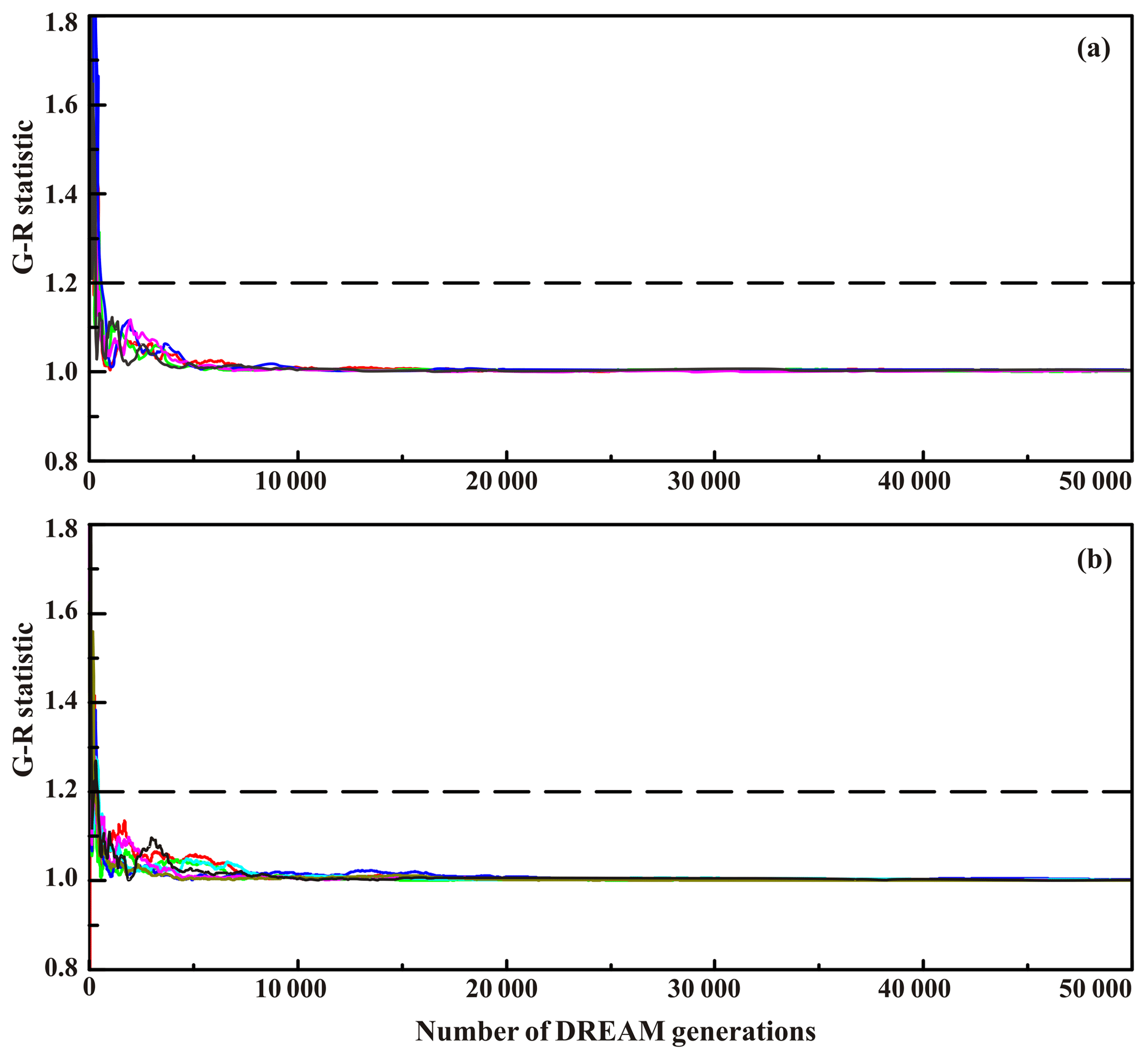
Figure 1Trace plots of the G–R statistic using DREAM for the PM model (a) and (b) the SW model. Different parameters are coded with different colors. The dashed line denotes the default threshold used to diagnose convergence to a limiting distribution.
Table 1Prior distributions and parameter limits for the PM, SW, PT–FC and AA models. The values are derived from the literature.
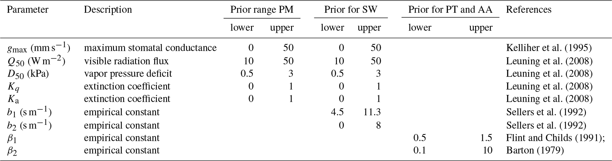
3.1 Parameter estimation
The PM model has five parameters, gmax, D50, Q50, Kq, and Ka; the SW model has seven parameters – the five used in the PM model and parameters b1 and b2. The PT–FC and AA models each include two parameters, denoted by β1 and β2 (Table 1). The prior probability density of each parameter is specified as an uniform distribution with the ranges listed in Table 1. A total of 50 000 realizations were generated with the DREAM algorithm, which was used to estimate the posterior probability density function of each parameter with the calibration period data from DOY 154 to DOY 202. In the calculations, the chain number, N, was equal to the number of parameters in the associated model. Therefore, N is equal to 5, 7, 2, and 2 for the PM, SW, PT–FC, and AA models, respectively. For each model, the first 10 000 samples were discarded as burn-in data, and the remaining 40 000 samples were used for calibration. In total, 40 000×N realizations were used to set up posterior density functions for each model. To illustrate the efficiency and convergence of DREAM for the ET models, Fig. 1 shows the trace plots of the G–R (Gelman and Rubin, 1992) statistic for each of the different parameters in the PM and SW models using a different color. The algorithm required about 8000 generations to make the G–R statistic close to 1.0 for the two models. The acceptance rates for the PM and SW models were about 15.3 % and 18.9 %, respectively.
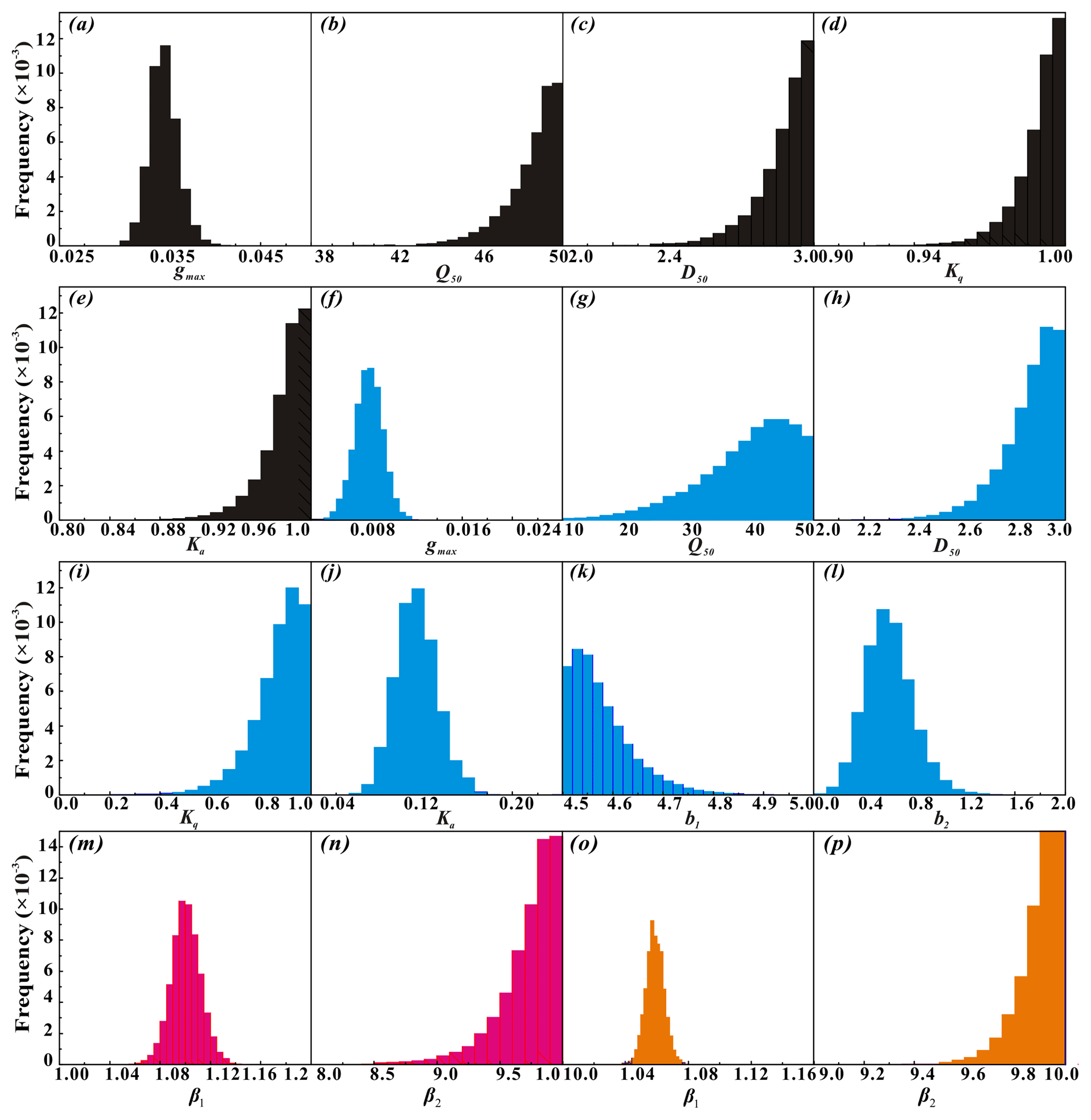
Figure 2(a–e), (f–l), (m–n), and (o–p) show histograms for the PM (black), SW (cyan), PT–FC (magenta), and AA (orange) models, respectively. These histograms are constructed from all chains for each model, and a total of 40 000×N realizations are simulated using DREAM. The x axes represent the prespecified limits of the parameters.
Table 2Maximum likelihood estimates (MLEs), mean estimates, 95 % high-probability intervals (lower limit, upper limit).
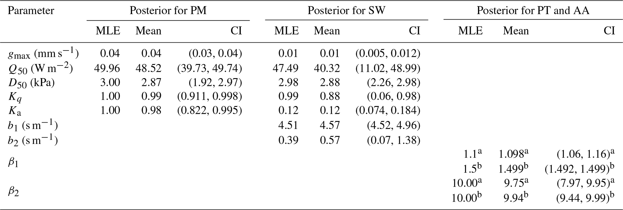
a PT–FC model; b AA model.
Histograms of the DREAM-derived marginal distributions of the parameters are presented in Fig. 2 and summarized in Table 2 by maximum likelihood estimates (MLEs), posterior medians, and 95 % probability intervals. Figure 2a–e, f–l, m–n, and o–p show histograms of the PM, SW, PT–FC, and AA models, respectively. Parameter gmax (Fig. 2a) in the PM model; parameters gmax, Ka, and b2 (Fig. 2f, j, l) in the SW model; and parameter β1 (Fig. 2m) in the PT–FC model and AA model (Fig. 2o) were well constrained and occupied a relatively small range. These parameters displayed a unimodal distribution and appeared approximately Gaussian. In contrast, the distributions of the other parameters differed significantly from a Gaussian distribution, as shown by the corresponding histograms. The distributions of all but one of these parameters concentrated most of the probability mass at their upper limits. The exception was parameter b1 for the SW model (Fig. 2k), which clearly does not follow a normal distribution, with most of the mass concentrated in the lower bounds. In contrast, Q50 was not only poorly constrained (Fig. 2g) but was also the upper-edge-hitting parameter in the SW model. Moreover, the corresponding distributions of the same parameter in different models were slightly different. For example, the mean of gmax in the PM model (0.04 mm s−1) was less than that in the SW model (0.01 mm s−1; Fig. 2a and f; Table 2) except that D50 in the PM and SW models and β2 in the PT–FC and AA models exhibited similar regions. It is interesting to observe that the distribution of Ka in the PM model (Fig. 2e) has a truncated distribution with highest probability mass at the upper bound, whereas the distribution of Ka in the SW model (Fig. 2j) tends to become approximately normal. Overall, the marginal posterior probability density function of most of the individual parameters occupied only a relatively small region compared with the uniform prior distributions and exhibited relatively large uncertainty reduction.
3.2 Performance of the models
The performance of each of the four ET models was evaluated over the course of the whole season in 2014. The calibrated parameters of the four models were used, and individual ET models were run to estimate the half-hourly λET values. Table 3 summarizes the statistical results for the performance of the models using the regression line slope, R2, RMSE, MBE, IA, and EF. The regressions between measured and modeled λET values and the MBE are shown in Figs. 3 and 4, respectively.
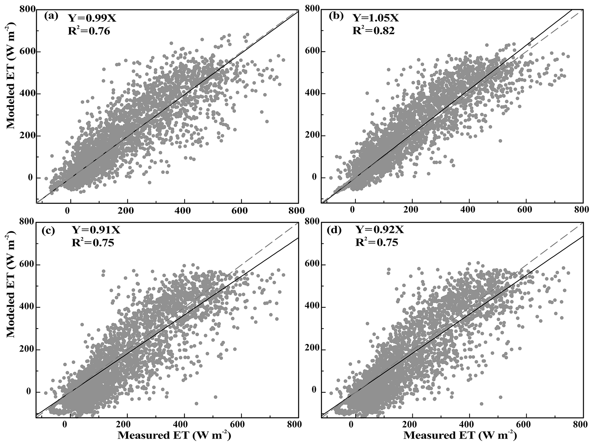
Figure 3Regressions between measured and modeled half-hourly ET values produced by different models from DOY 154 to DOY 270: (a) PM, (b) SW, (c) PT–FC, and (d) AA. The regressions are Y=0.99X (R2=0.76), Y=1.05X (R2=0.82), Y=0.91X (R2=0.75), and Y=0.92X (R2=0.75) for the PM, SW, PT–FC, and AA models, respectively.
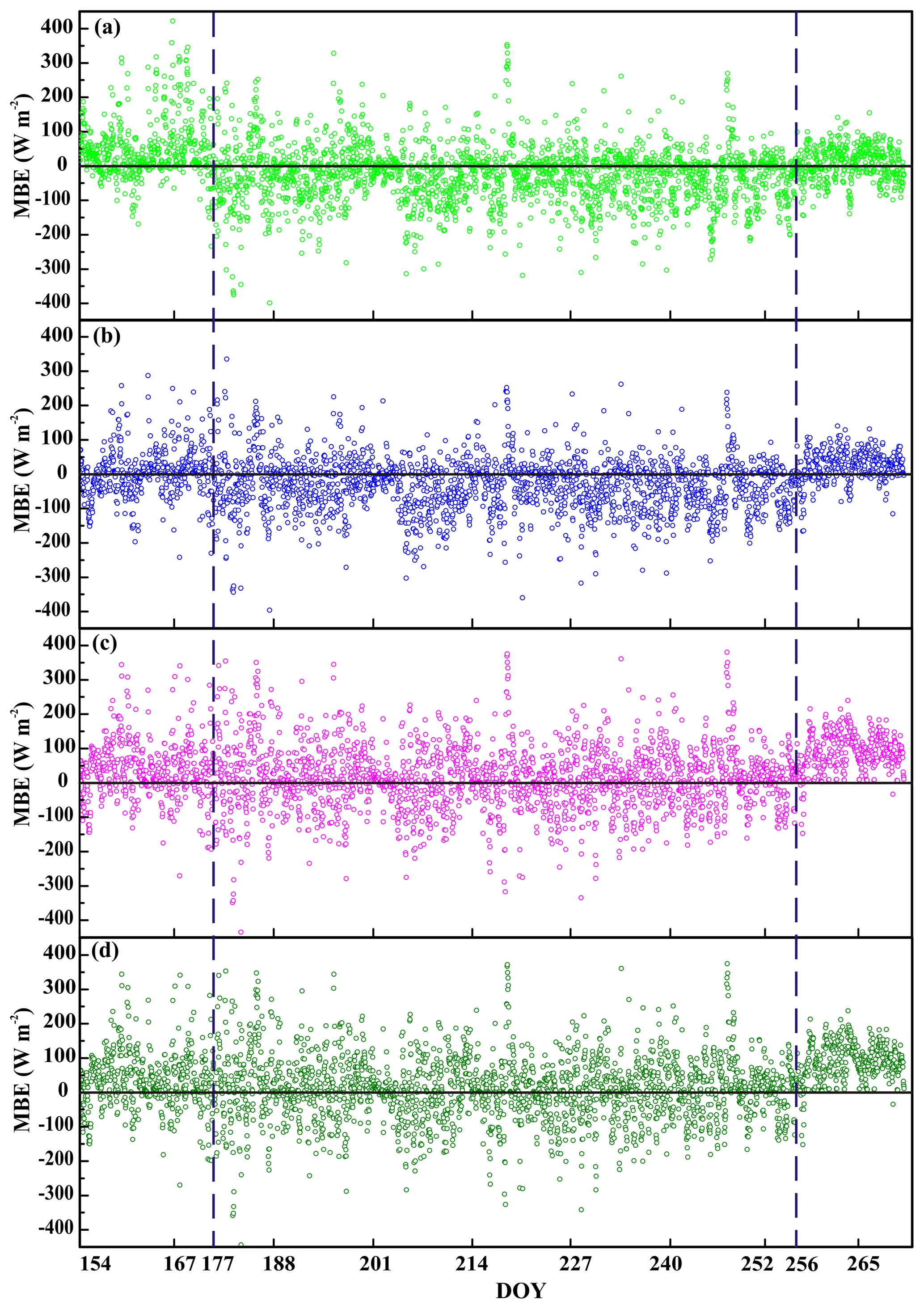
Figure 4Mean bias error (MBE) of predicted and observed ET values for (a) PM, (b) SW, (c) PT–FC, and (d) AA models from DOY 154 to DOY 270. Parameters used for prediction are estimated by DREAM with the dataset for the calibration period from DOY 154 to DOY 202.
Table 3Slope and coefficient of determination (R2) of regression between measured and modeled half-hourly evapotranspiration values, and statistics of root mean square error (RMSE), mean bias error (MBE), index of agreement (IA), model efficiency (EF) and Logarithm of BME for the four ET models.
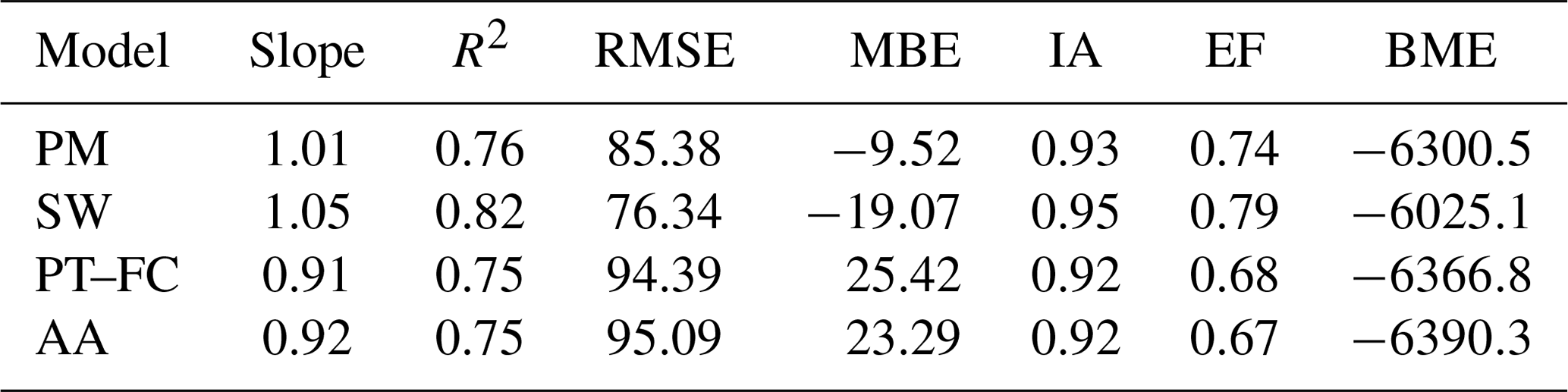
In general, the four models produced slightly better fits to the measured λET for all the seasons with R2 larger than 0.75 (Fig. 3). However, obvious discrepancies in the predictions made by the models were detected by comparing measured and modeled λET. According to the regression line slope and MBE, the PM model overestimated ET by 1 %, with an MBE of −9.52 W m−2, and the SW model overestimated ET by 5 %, with a relatively higher MBE of −19.07 W m−2 compared to the PM model. The PT–FC and AA models tended to underestimate λET by 9 % and 8 %, with an MBE of 25.42 and 23.29 W m−2, respectively. From a comparison between the slope and MBE, the PM model performance was higher than that of the other three models, with a slope almost equal to 1 and a relatively lower MBE. The SW model was ranked second, while the performance of the AA model was slightly higher than that of the PT–FC model. However, if R2, RMSE, IA, and EF were used to evaluate performance, the SW model had the best overall performance, with R2=0.83, RMSE = 76.34 W m−2, IA = 0.95, and EF = 0.79. The second-best model was the PM model, the PT–FC model was ranked third, and the AA model ranked fourth. Based on the analysis of these traditional error metrics, the PT–FC and AA models yielded similar results. The observed and modeled λET for the four ET models were tightly grouped along the regression lines (Fig. 3), and the PT–FC and AA models had similar modeled ET values with a similar degree of point scattering along the regression lines (Fig. 3 and d).
Figure 4 shows that large seasonal variations arise in the MBE for the four ET models. From the variations in the MBE, the estimated λET values for all models were generally lower than the measured values before the early jointing stage of maize growth (DOY 154–177; left dashed line) and after the late maturity stage (DOY 256–265; right dashed line) with the corresponding LAI < 2.5 m2 m−2. More positive MBE values for the PT–FC and AA models after the late maturity stage indicate their underestimated performances; however, these estimations appeared to be even more consistent, with a symmetrical scattering of points along the 0–0 line (Fig. 4c and d) during DOY 177–256 and with LAI > 2.5 m2 m−2.
3.3 Comparison of the models using BME
Since there is currently no theoretical method for selecting power posterior β values, we determined these values using empirical but straightforward methods. For any power coefficient of β∈[0, 1], a sample was drawn from the distribution pβ (Eq. 23) through running DREAM. Although adding more βk values might improve the BME estimation, this was not done because of the computational cost. For each βk value, at least 150 000 DREAM simulations were large enough to ensure convergence. Figure 5 shows the evolution of ln p(D|θ, M) for the four models as a function of β for a dataset covering the entire period. The BME for the SW model was substantially larger than that for the other three models, and the BME for the AA model was the smallest. The BME-based model ranking (from the best to the worst) is SW, PM, PT–FC, and AA. The PT–FC and AA models, which consist of the same number of parameters, had similar potential patterns of evolution with respect to the coefficient βk. The results illustrate that with the addition of parameters, the model complexity and the model performance are both increased.

Figure 5Variation of the mean posterior expectation of the potential yk with βk for the PM, SW, PT–FC, and AA models.
4.1 Parameter uncertainty analysis
With regard to the efficiency of the DREAM algorithm, the acceptance rates of the PM (15.3 %) and SW (18.9 %) models were much higher than those obtained by some MCMC algorithms that have been used in previous studies (Sadegh and Vrugt, 2014). The posterior parameter bounds exhibit a larger reduction using the DREAM algorithm compared with other studies using the Metropolis–Hastings algorithm. This demonstrates that DREAM could efficiently handle problems involving high dimensionality, multimodality, and nonlinearity.
The results showed that the assumed prior uncertainty ranges from most parameters in the four models were significantly reduced. This indicates that the observed ET data contained sufficient information for estimating these parameters. Surface conductance gs and modeled ET in the PM model are relatively insensitive to Q50, D50, and Kq. Hence, these parameters could not be well constrained, and further relaxing the ranges for these parameters could not result in physically realistic behavior of the model. The calculation of in the SW model is the same as in the PM model, and thus and modeled ET in the SW model are also insensitive to the parameters of Q50, D50, and Kq. Therefore, these three parameters were also not well constrained in the SW model. In addition, the uncertainties present in the edge-hitting parameters may be the outcome of model biases or EC-measured ET data errors or the characteristic timescale of parameters governing the processes affecting ET being not exactly on the order of half-hours (Braswell et al., 2005). For example, Q50 and D50 govern changes in visible radiation flux and the humidity deficit at which stomatal conductance is half its maximum value, respectively, and these parameters may change over a shorter or longer timescale than half-hours.
The ecophysiological parameter gmax is a variable in the equation in both the PM and SW models, but this parameter is sensitive to and has a significant impact on the evaluated ET. Its effect is relatively independent compared to the other meteorological parameters in the models, and therefore this parameter was well specified in the PM and SW models. The posterior mean value of gmax (0.04 m s−1) in the PM model from our study was close to that (0.05 m s−1) reported in northwestern China (Li et al., 2013; Zhu et al., 2014), but gmax (0.01 m s−1) in the SW model was less than the reported value. Parameter β1 was well constrained in the PT–FC and AA models because it was relatively independent and did not directly relate to other observed variables.
Parameter Ka implicitly appears in the surface conductance equation (Eq. 2) in the PM model, and Ka is insensitive to gs and modeled ET (Leuning et al., 2008). In contrast, Ka is contained in the equation of net radiation flux into the substrate (Eq. 10) in the SW model. This parameter can explicitly partition the total available energy into that absorbed by the canopy and by the soil in the SW model. An analysis of Eq. (10) found that the variation of Ka could not only account for the extinction effect but also correct the energy forcing data errors. This also meant that the estimated value of Ka using calibration data was actually not just the true extinction coefficient but also included the energy imbalance correction in the SW model. From this analysis, we could see that Ka not only involved the distribution of energy between the canopy and the soil surface but also the energy imbalance. Therefore, parameter Ka has a great influence on the performance of the SW model. This is why Ka is poorly constrained in the PM model but well constrained in the SW model. To further illustrate the insights regarding the influence of parameter Ka on the performance of the SW model, we calibrated the SW model again and reran the model with a constant value of Ka. The results showed a significant reduction in model performance when Ka was held constant. This implied that the main reason for the SW model outperforming the PM model in our study was not only the more physically rigorous structure of the SW model but also the key parameter Ka being well constrained in the SW model.
In general, parameters related to soil surface resistance in the SW model were well evaluated, while parameters related to canopy surface resistance in PM and SW models were poorly estimated. Therefore, using a reliable canopy surface resistance equation in the ET model was crucial for improving its performance. In addition, in our study, the traditional approach was used to quantify the uncertainty, which assumed that the uncertainty mainly arose because of the parameter uncertainty. However, this method cannot explicitly consider errors in the input data and model structural inadequacies. This is unrealistic for real applications, and it is desirable to develop a more reliable inference method to treat all sources of uncertainty separately and appropriately (Vrugt et al., 2008). Moreover, simultaneous direct measurement by the micro-lysimeter of sap flow and daily soil evaporation will further help to constrain the model parameters.
4.2 Evaluation and selection of the models
In this study, the traditional statistical measures and BME were chosen to evaluate and compare the performance of four ET models. From the respective composition of these measures, the statistical measures can be divided into residual-based metrics (such as regression slope and MBE) and squared-residual-based measures (such as R2, RMSE, IA, and EF). The rankings of the models obtained using the same type of metric (residual-based or squared-residual-based) are similar. Slope and MBE, for example, which are both residual-based measures, produce identical rankings. However, the rankings produced by metrics of different types are not the same. For example, the PM model outperforms the SW model according to the residual-based metrics, but the performance of the PM model is worse than the SW model based on the squared-residual-based measures. The comparative analysis shows consistency between BME and the squared-residual-based metrics (hence the residual-based metrics disagreed with the BME measures). This reveals that the more complex SW model is the best model based on BME and squared-residual-based statistics. The rank order of overall performance of the models from best to worst is SW, PM, PT–FC, and AA.
Previous studies showed that BME evaluated by TI provided estimates similar to the true values and selected the true model if the true model was included within the candidate models (Marshall et al., 2005; Lartillot and Philippe, 2006). Meanwhile, some have argued that Bayesian analysis would choose the simplest model (Jefferys and Berger, 1992; Xie et al., 2011) because of the best trade-off between good fit with the data and model complexity (Schöniger et al., 2014). In this case, the most complex SW model had the highest BME and was chosen as the model with the best performance. This probably resulted from the fact that the complex SW model is indeed the most reliable model among the alternative ET models and can provide a good fit to justify its higher complexity. The SW model is a two-layer model and simulates soil evaporation and plant transpiration separately, whereas the PM model is a single-layer model in which the plant transpiration and soil evaporation cannot be separated (Monteith, 1965). The PT–FC model is a simplified version of the PM model and only requires meteorological and radiation information (Priestley and Taylor, 1972), whereas the AA model only relies on the feedback between actual ET and potential ET (Brutsaert and Stricker, 1979).
The results indicate that the squared-residual-based measures yielded the same rank order as the BME consistently, which makes the squared-residual-based metrics seem to identify a reasonable rank order. However, this has not been the general case, since the error metrics and BME belong to different types of model selection and because there are differences in the behavior and optimality of the two types of model selection. BME is a consistent model selection that tries to identify which of the models produced the observed data. Conversely, nonconsistent model selection uses the available data to estimate which of the models might be best in predicting future data. In fact, the error metrics are essentially nonparsimonious model selection, which is a special case of nonconsistent model selection. The simple traditional statistical measures were known to usually provide a biased view of the efficacy of a model (Kessler and Neas, 1994; Legates and McCabe, 1999), where only the goodness of fit is used for rating models without penalizing the model complexity, thus lacking consistency for the selected model (Höge et al., 2018). In addition, sensitivity to outliers is associated with these metrics and leads to relatively high values due to the squaring of the residual terms (Willmott, 1981). Furthermore, these traditional statistical metrics ignore the priors, which are in fact used in Bayesian analysis. The PT–FC and AA models provide identical estimates of R2 and IA. This is most likely because both models had the same dimension and a similar model structure. Marshall et al. (2005) argued that EF would provide an incorrect conclusion, and Samani et al. (2018) suggested that RMSE would select the complex model as the best performing model. As for the slope and MBE, the rankings produced by these residual-based metrics were in obvious disagreement with the one based on BME. Part of the lower simulation values could be counterbalanced by the higher values of that in the slope and MBE methods; thus these criteria provide an erroneous and unreliable evaluation of the models. Therefore, the squared-residual-based and residual-based measures were not certain in providing reasonable results in terms of model ranking. The consistency between BME and the squared-residual-based metrics only indicates that the optimal model evaluated by BME would also provide the best predictions, and thus consistent model selection should also be asymptotically efficient (Leeb and Pötscher, 2009; Shao, 1997).
4.3 Analysis of model–data mismatch
Conceptual and structural inadequacies of the hydrological model together with measurement errors of the model input (forcing) and output (calibration) data introduce errors in the estimated parameters and model simulations (Laloy et al., 2015). Hydrological systems are indeed heavily input-driven, and errors in forcing data can dramatically impair the quality of calibration results and model output (Bardossy and Das, 2008; Giudice et al., 2016). Measurement errors occur for a variety of reasons, including unreasonable gap filling in rainy days; dew and fog; inadequate areal coverage of point-scale soil water measurement; mechanical limitations of the EC system; and inaccurate measurements of wind speed, soil water, radiation, and vapor pressure deficit. The ET process is described using equations that can only capture parts of the complex natural processes, and any ET model is an inherent simplification of the real system. These inadequacies can thus lead to biased parameters and implausible predictions.
In our study, the results indicated that the PM and SW models overestimated the half-hourly ET compared to the measured ET. Several studies also indicated that ET was overestimated by the PM model (Fisher et al., 2005; Ortega-Farias et al., 2006; Li et al., 2015) and the SW model (Li et al., 2013, 2015; Zhang et al., 2008). Possible reasons for the inaccurate estimates included the following: (1) anisotropic turbulence with weak vertical and strong horizontal fluctuation leads to energy imbalance. The total turbulent heat flux was lower by ∼10 %–30 % compared to the available energy in many land surface experiments (Tsvang et al., 1991; Beyrich et al., 2002; Oncley et al., 2007; Foken et al., 2010) and influx networks (Franssen et al., 2010). Liang et al. (2017) also showed an energy imbalance result in the semiarid area in China and indicated that the energy balance closure ratio ranged from 0.52 to 0.90 during the day, whereas it was about 0.25 at night. However, the measured ET only included vertical flux and not horizontal flux, leading to the measured ET being lower than that of ET predicted by the PM and SW models using the available energy. (2) The absence of a mechanistic representation of the physiological response to plant hydrodynamics makes it difficult for the available ET models to resolve the dynamics of intradaily hysteresis, producing patterns of diurnal error, while the imbalance or lack of between-leaf water demand and soil water supply imposes hydrodynamic limitations on stomatal conductance (Thomsen et al., 2013; Zhang et al., 2014; Matheny et al., 2014). Li et al. (2015) also concluded that neglecting the restrictive effect of the soil on water transport in empirical canopy resistance equations can result in large errors in the partial canopy stage. However, these equations can estimate ET accurately under the full canopy stage (Alves and Pereira, 2000; Katerji and Rana, 2006; Katerji et al., 2011; Rana et al., 2011). Li et al. (2015) showed that the PM model combined with canopy resistance overestimated maize ET during the partial and dense canopy stages by 16 % and 13 %, respectively. Moreover, in a study of ET in vineyards, Leuning et al. (2008) found that the PM model coupled with canopy resistance overestimated ET during the entire growth stage by 29 %.
The estimates for ET produced by the PT–FC and AA models were generally lower than the measured values during the entire season. In addition, the four models also underestimated ET during periods of partial cover (LAI < 2.5 m2 m−2). The PT–FC and AA models consistently underestimated ET, especially during the late maturity stage. The underestimation probably resulted from the following: (1) nonclassical situations, such as the oasis effect, may occur in the study area. Strong evaporation from the moist ground and plants results in latent heat cooling. However, this upward latent heat flux was opposed by a downward sensible heat flux from the warm air to the cool ground, and thus the latent heat flux was positive while the sensible heat flux is negative. Therefore, the latent heat flux can be greater in magnitude than the solar heating because of the additional energy extracted from the warm air by evaporation (Stull, 1988). (2) The lack of mechanistic representation of rainfall interception in ET models probably led to inaccurate simulation for periods soon after rainy days. Bohn and Vivoni (2016) found that evaporation of canopy interception accounted for 8 % of the annual ET across the North American monsoon region. Comparing the AA and PT–FC models, the former includes forcing data of available radiation, soil water content, and relative humidity, but the PT–FC model only requires available radiation and soil water content and is independent of relative humidity. However, the similar statistical results and similar degrees of MBE scatter indicate that relative humidity has little influence on the AA model simulation. The consistent and consecutive underestimations of ET by the PT–FC and AA models during the late maturity stage show that the model–data disagreement is not caused by regional advection and rainfall interception because atmospheric processes and thermally induced circulation can only occur at certain times and during certain days. Therefore, we think that the consistent underestimation of ET by the PT–FC and AA models results primarily from conceptual and structural inadequacies, energy imbalance, and soil water stress. Although the PM and SW models share a common theoretical basis and the PT–FC model is a simplification of the PM model, these models perform significantly differently. Part of the overestimation of ET by the PM and SW models, caused by coupling with the canopy resistance, may be offset by underestimation caused by energy imbalance and soil water stress. However, underestimation of ET by the PT–FC and AA models cannot be counterbalanced by overestimation during the later maturity stage because the PT–FC and AA models are independent of the canopy resistance. Consequently, the half-hourly patterns of errors in the estimates of ET by the PM and SW models are characterized by symmetry and a low degree of scatter, but the PT–FC and AA models exhibit consistently asymmetrical error patterns. By contrast, other studies showed that the PM model (Kato et al., 2004) and the SW model (Chen et al., 2015) underestimated half-hourly ET. As for the PT–FC and AA models, some studies reported that the PT–JPL (Zhang et al., 2017) and the AA model showed an overall poor performance (Zhang et al., 2017), while other studies have indicated that the AA method performed well for both maize and canola crops (Liu et al., 2012). Therefore, the performance of the four ET models appears to vary not only for different crops and locations but also for different meteorological, physiological, and soil conditions. Moreover, the performance is also related to the stage of crop growth. Note that these conclusions about the ET models evaluation are derived from traditional error metrics rather than those based on BME model selection. It would be desirable to use available data from other study areas or from other crops for BME-based model selection to confirm whether the SW model is the optimal model under other conditions. Overall, combined with the parameter uncertainty analysis described in Sect. 4.1, we conclude that energy imbalance and energy interaction between the canopy and soil surface have a greater impact on the model performance; thus, explicitly treating energy error and incorporating the elements of existing hydrologic theory about energy interaction between the canopy and surface or conceptually correcting the energy interaction are a practicable option for model improvement and application.
This study illustrated the application of the Bayesian approach on the statistical analysis and model selection of four widely used ET models. The results showed that the DREAM algorithm successfully reduced the assumed prior uncertainties for most of the parameters in the four models. In the model calibration, the key parameters which had a significant influence on ET simulations were well constrained. The main reasons for the outperforming of SW model were its physically rigorous structure and the extinction coefficient parameter, which is sensitive and has a significant impact on the performance of the model, being well constrained. BME is a consistent model selection for identifying the best fitting to the observed data. Although the squared-residual-based metrics, including R2, IA, RMSE, and EF, produced a ranking identical to that of BME, it must be noted that these squared-residual-based metrics do not allow using prior information and do not penalize the model complexity when comparing the models. Therefore, some caution is needed when using these statistical methods to compare different models.
The model–data discrepancies were analyzed to facilitate model improvement after Bayesian model calibration and comparison. The results indicate that the discrepancies arose mainly as a result of energy imbalance caused by anisotropic turbulence, additional energy induced by advection processes, the absence of a mechanistic representation of the physiological response to plant hydrodynamics and the energy interaction between the canopy and surface. Among these causes, energy imbalance and additional energy are related to forcing data errors rather than to an unreasonable model structure. Thus, understanding the process of the physiological response to plant hydrodynamics, and the interaction between the canopy and surface is essential for improving the performance of evapotranspiration models. Overall, the applications of Bayesian calibration, Bayesian model evaluation, and analysis of model–data discrepancies in our study provide a promising framework for reducing uncertainty and improving the performance of ET models. It would be desirable to confirm whether the SW model is the optimal model using data of other crops or other climate regions.
The eddy covariance flux, meteorological, and other data used in this study are from Heihe Watershed Allied Telemetry Experimental Research (HiWATER) (http://heihedata.org/hiwater, last access: 6 January 2016).
| A | Available energy for the whole canopy (W m−2) |
| As | Available energy for the soil surface (W m−2) |
| Rn | Net radiation fluxes into the canopy (W m−2) |
| Rns | Net radiation flux into the substrate (W m−2) |
| G | Soil heat flux (W m−2) |
| λET | Sum of the latent heat flux from the crop (λT) and soil (λE; W m−2) |
| ETc | Canopy transpiration (W m−2) |
| ETs | Soil evaporation (W m−2) |
| Cc | Canopy resistance coefficient (dimensionless) |
| Cs | Soil surface resistance coefficient (dimensionless) |
| LAI | Leaf area index |
| Q50 | Visible radiation flux when stomatal conductance is half its maximum value (W m−2) |
| D50 | Vapor pressure deficit at which stomatal conductance is half its maximum value (kPa) |
| Da | Vapor pressure deficit at the reference height (; kPa) |
| Qh | Flux density of visible radiation at the top of the canopy (W m−2) |
| Kq | Extinction coefficient |
| Ka | Extinction coefficient |
| f | Fraction of evaporation soil and total evaporation |
| λ | Latent heat of water evaporation (MJ kg−1) |
| Δ | Slope of the saturated vapor pressure curve (Pa K−1) |
| γ | Psychrometric constant (kPa K−1) |
| ρ | Density of air (kg m−3) |
| k | Karman constant (0.41) |
| es | Saturated vapor pressure (kPa) |
| ea | Actual vapor pressure (kPa) |
| q* | Saturation-specific humidity at air temperature (kg kg−1) |
| q | Specific humidity of the atmosphere (kg kg−1) |
| b1 | Empirical constant (s m−1) |
| b2 | Empirical constant (s m−1) |
| β1 | Empirical constant |
| β2 | Empirical constant |
| θ | Soil water content (m3 m−3) |
| θa | Critical water content at which plant stress starts (m3 m−3) |
| θb | Water content at the wilting point (m3 m−3) |
| θr | Residual soil water content (m3 m−3) |
| θs | Saturated water content (m3 m−3) |
| Θ | Relative water saturation |
| d | Zero-plane displacement height (m) |
| zm | Height of the wind speed and humidity measurements (3 m) |
| z0 m | Roughness length governing the transfer of momentum (m) |
| z0 v | Roughness length governing the transfer of water vapor (m) |
| h | Canopy height (m) |
| uz | Wind speed at height zm (m s−1) |
| ga | Aerodynamic conductance (m s−1) |
| gs | Surface conductance (m s−1) |
| gmax | Maximum stomatal conductance of leaves at the top of the canopy (m s−1) |
| Canopy conductance (m s−1) | |
| ra | Aerodynamic resistance (s m−1) |
| Aerodynamic resistance between canopy source height and a reference level (s m−1) | |
| Aerodynamic resistance between the substrate and the canopy source height (s m−1) | |
| Bulk boundary layer resistance of the vegetation element in the canopy (s m−1) | |
| Surface resistance of the canopy (s m−1); | |
| Bulk stomatal resistance of the canopy (s m−1) |
The posterior probability distribution of the parameter is calculated by Bayes' theorem:
where π(θ|M) represents the prior density of θ under model M, p(D|θ, M) is the joint likelihood of model M and its parameters θ, and the marginal likelihood, or Bayesian model evidence (BME), is
The likelihood function, p(D|θ, M), used for parameter estimation, is specified according to the distributions of observation errors. Error e(t) in each observation D(t) at time t is expressed by
Assuming that e(t) follows a Gaussian distribution with a zero mean, the likelihood function can be expressed as
where n is the number of observations and σ represents the error variances.
In this study, we used the DREAM algorithm (Vrugt et al., 2008, 2009) to explore the ET models' parameter space and to estimate BME. The DREAM sampling scheme is an adaptation of the global optimization algorithm of a shuffled complex evolution Metropolis (SCEM-UA). This algorithm was described in more detail in Vrugt et al. (2008, 2009).
GW and XZ designed the experiments. NY and FK carried them out. MY developed the model selection scheme. GW performed the simulations. GW and XZ prepared the paper, with contributions from all co-authors.
The authors declare that they have no conflict of interest.
We thank Ying Guo, Huihui Dang, Jun Dong for the data collection and analysis. All observed data used in this study are from Heihe Watershed Allied Telemetry Experimental Research (HiWATER). We thank all the staff who participated in HiWATER field campaigns. Considerate and helpful comments by anonymous reviewers have considerably improved the paper.
This research has been supported by the National Natural Science Foundation of China (grant nos. 41471023 and 41702244), the Department of Energy (grant no. DE-SC0019438), and the National Science Foundation – Division of Earth Science grant no. 1552329.
This paper was edited by Bill X. Hu and reviewed by Dan Lu and two anonymous referees.
Allen, R. G., Perista, L. S., Raes, D., and Smith, M.: Crop Evapotranspiration – Guidelines for Computing Crop Water Requirements; FAO Irrigation and Drainage papers 56, FAO – Food and Agriculture Organization of the United Nations, Rome, 1998.
Alves, I. and Pereira, L. S.: Modeling surface resistance from climatic variables?, Agr. Water Manage., 42, 371–385, 2000.
Aubinet, M., Grelle, A., Ibrom, A., Rannik, Ü., Moncrieff, J., and Foken, T.: Estimates of the annual net carbon and water exchange of forests: the euroflux methodology, Adv. Ecol. Res., 30, 113–175, 2000.
Baldocchi, D. D.: Assessing the eddy covariance technique for evaluating carbon dioxide exchange rates of ecosystems: past, present and future, Global Change. Biol., 9, 479–492, 2003.
Bardossy, A. and Das, T.: Influence of rainfall observation network on model calibration and application, Hydrol. Earth Syst. Sci., 12, 77–89, https://doi.org/10.5194/hess-12-77-2008, 2008.
Barton, I. J.: A Parameterization of the Evaporation from Nonsaturated Surfaces, J. Appl. Meteorol., 18, 43–47, 1979.
Beyrich, F., Richter, S. H., Weisensee, U., Kohsiek, W., Lohse, H., de Bruin, H. A. R., Foken, T., Göckede, M., Berger, F., Vogt, R., and Batchvarova, E.: Experimental determination of turbulent fluxes over the heterogeneous litfass area: selected results from the litfass-98 experiment, Theor. Appl. Climatol., 73, 19–34, https://doi.org/10.1007/s00704-002-0691-7, 2002.
Bohn, T. J. and Vivoni, E. R.: Process-based characterization of evapotranspiration sources over the North American monsoon region, Water Resour. Res., 52, 358–384, https://doi.org/10.1002/2015WR017934, 2016.
Bonan, G.: Ecological climatology: concepts and applications, Cambridge University Press, Cambridge, 2008.
Braswell, B. H., Sacks, W. J., Linder, E., and Schimel, D. S.: Estimating diurnal to annual ecosystem parameters by synthesis of a carbon flux model with eddy covariance net ecosystem exchange observations, Global Change Biol., 11, 335–355, 2005.
Brutsaert, W.: Hydrology: An Introduction, Cambridge University Press, Cambridge, 2005.
Brutsaert, W. and Stricker, H.: An advection-aridity approach to estimate actual regional evapotranspiration, Water Resour. Res., 15, 443–450, 1979.
Chen, D. Y., Wang, X., Liu, S. Y., Wang, Y. K., Gao, Z. Y., Zhang, L. L., Wei, X. G., and Wei, X. D.: Using Bayesian analysis to compare the performance of three evapotranspiration models for rainfed jujube (Ziziphus jujuba Mill.) plantations in the Loess Plateau, Agr. Water. Manage., 159, 341–357, 2015.
Elshall, A. S., Ye, M., Pei, Y., Zhang, F., Niu, G. Y., and Barron-Gafford, G. A.: Relative model score: A scoring rule for evaluating ensemble simulations with application to microbial soil respiration modeling, Stoch. Environ. Res. A., https://doi.org/10.1007/s00477-018-1592-3, in press, 2018.
Ershadi, A., Mccabe, M. F., Evans, J. P., Chaney, N. W., and Wood, E. F.: Multi-site evaluation of terrestrial evaporation models using fluxnet data, Agr. Forest Meteorol., 187, 46–61, 2014.
Ershadi, A., McCabe, M .F., Evans, J. P., and Wood, E. F.: Impact of model structure and parameterization on Penman–Monteith type evaporation models, J. Hydrol., 525, 521–535, 2015.
Fisher, J. B., DeBiase, T. A., Qi, Y., Xu, M., and Goldstein, A. H.: Evapotranspiration models compared on a Sierra Nevada forest ecosystem, Environ. Model. Softw., 20, 783–796, 2005.
Flint A. L. and Childs, S. W.: Use of the Priestley–Taylor evaporation equation for soil water limited conditions in a small forest clearcut, Agr. Forest Meteorol., 56, 247–260, 1991.
Foken, T., Mauder, M., Liebethal, C., Wimmer, F., Beyrich, F., Leps, J. P., Raasch, S., DeBruin, H. A. R., Meijninger, W. M. L., and Bange, J.: Energy balance closure for the LITFASS-2003 experiment, Theor. Appl. Climatol., 101, 149–160, https://doi.org/10.1007/s00704-009-0216-8, 2010.
Franssen, H. J. H., Stöckli, R., Lehner, I., Rotenberg, E., and Seneviratne S. I.: Energy balance closure of eddy-covariance data: A multisite analysis for European FLUXNET stations, Agr. Forest Meteorol., 150, 1553–1567, https://doi.org/10.1016/j.agrformet.2010.08.005, 2010.
Gelman, A. and Meng, X. L.: Simulating normalizing constants: From importance sampling to bridge sampling to path sampling, Stat. Sci., 13, 163–185, 1998.
Gelman, A. and Rubin, D. B.: Inference from iterative simulation using multiple sequences, Stat. Sci., 7, 457–472, 1992.
Giudice, D., Albert, C., Rieckermann, J., and Reichert, P.: Describing the catchment-averaged precipitation as a stochastic process improves parameter and input estimation, Water Resour. Res., 52, 3162–3186, https://doi.org/10.1002/2015WR017871, 2016.
Höge, M., Wöhling, T., and Nowak, W.: A primer for model selection: The decisive role of model complexity, Water Resour. Res., 54, 1688–1715, https://doi.org/10.1002/2017WR021902, 2018.
Jefferys, W. H. and Berger, J. O.: Sharpening Ockham's razor on a Bayesian strop, Am. Sci., 89, 64–72, 1992.
Kashyap, R. L.: Optimal choice of AR and MA parts in autoregressive moving average models, IEEE T. Pattern Anal. Mach. Intell., 4, 99–104, 1982.
Katerji, N. and Rana, G.: Modelling evapotranspiration of six irrigated crops under Mediterranean climate conditions, Agr. Forest Meteorol., 138, 142–155, 2006.
Katerji, N., Rana, G., and Fahed, S.: Parameterizing canopy resistance using mechanistic and semi-empirical estimates of hourly evapotranspiration: critical evaluation for irrigated crops in the Mediterranean, Hydrol. Process., 25, 117–129, 2011.
Kato, T., Kimura, R., and Kamichika, M.: Estimation of evapotranspiration, transpiration ratio and water-use efficiency from a sparse canopy using a compartment model, Agr. Water Manage., 65, 173–191, 2004.
Kelliher, F. M., Leunig, R., Raupach, M. R., and Schulze, E. D.: Maximum conductances for evaporation from global vegetation types, Agr. Forest Meteorol., 73, 1–16, 1995.
Kessler, E. and Neas, B.: On correlation, with applications to the radar and raingage measurement of rainfall, Atmos. Res., 34, 217–229, 1994.
Laloy, E., Linde, N., Jacques, D., and Vrugt, J. A.: Probabilistic inference of multi-Gaussian fields from indirect hydrological data using circulant embedding and dimensionality reduction, Water Resour. Res., 51, 4224–4243, https://doi.org/10.1002/2014WR016395, 2015.
Lartillot, N. and Philippe, H.: Computing Bayes factors using thermodynamic integration, Syst. Biol., 55, 195–207, 2006.
Leeb, H. and Pötscher, B. M.: Model selection, Springer, Berlin, Germany, 889–925, https://doi.org/10.1007/978-3-540-71297-8-39, 2009.
Legates, D. R. and McCabe, G. J.: Evaluating the use of “goodnessof-fit” measures in hydrologic and hydroclimatic model validation, Water Resour. Res., 35, 233–241, 1999.
Leuning, R., Zhang, Y. Q., Rajaud, A., Cleugh, H., and Tu, K.: A simple surface conductance model to estimate regional evaporation using MODIS leaf area index and the Penman–Monteith equation, Water Resour. Res., 44, W10419, https://doi.org/10.1029/2007WR006562, 2008.
Liang, J., Zhang, L., Cao, X., Wen, J., Wang, J., and Wang, G.: Energy balance in the semiarid area of the Loess Plateau, China, J. Geophys. Res.-Atmos., 122, 2155–2168, https://doi.org/10.1002/2015JD024572, 2017.
Li, S., Kang, S., Zhang, L., Ortega-Farias, S., Li, F., Du, T., Tong, L., Wang, S., Ingman, M., and Guo, W.: Measuring and modeling maize evapotranspiration under plastic film-mulching condition, J. Hydrol., 503, 153–168, 2013.
Li, S., Zhang, L., Kang, S., Tong, L., Du, T., Hao, X., and Zhao, P.: Comparison of several surface resistance models for estimating crop evapotranspiration over the entire growing season in arid regions, Agr. Forest Meteorol., 208, 1–15, 2015.
Li, X., Cheng, G. D., Liu, S. M., Xiao, Q., Ma, M. G., Jin, R., Che, T., Liu, Q. H., Wang, W. Z., Qi, Y., Wen, J. G., Li, H. Y., Zhu, G. F., Guo, J. W., Ran, Y. H., Wang, S. G., Zhu, Z. L., Zhou, J., Hu, X. L., and Xu, Z. W.: Heihe Watershed Allied Telemetry Experimental Research (HiWATER): Scientific objectives and experimental design, B. Am. Meteorol. Soc., 94, 1145–1160, 2013.
Liu, G., Liu, Y., Hafeez, M., Xu, D., and Vote, C.: Comparison of two methods to derive time series of actual evapotranspiration using eddy covariance measurements in the southeastern Australia, J. Hydrol., 454–455, 1–6, 2012.
Liu, P., Elshall, A. S., Ye, M., Beerli, P., Zeng, X., Lu, D., and Tao, Y.: Evaluating marginal likelihood with thermodynamic integration method and comparison with several other numerical methods, Water Resour. Res., 52, 734–758, https://doi.org/10.1002/2014WR016718, 2016.
Liu, S. M., Xu, Z. W.,Wang,W. Z., Jia, Z. Z., Zhu, M. J., Bai, J., and Wang, J. M.: A comparison of eddy-covariance and large aperture scintillometer measurements with respect to the energy balanceclosure problem, Hydrol. Earth Syst. Sci., 15, 1291–1306, https://doi.org/10.5194/hess-15-1291-2011, 2011.
Marshall, L., Nott, D., and Sharma, A.: Hydrological model selection: A Bayesian alternative, Water Resour. Res., 41, 3092–3100, https://doi.org/10.1029/2004WR003719, 2005.
Matheny, A. M., Bohrer, G., Stoy, P. C., Baker, I. T., Black, A. T., Desai, A. R., Dietze, M. C., Gough, C. M., Ivanov, V. Y., Jassal, R. S., Novick, K. A., Schäfer, K. V. R., and Verbeeck, H.: Characterizing the diurnal patterns of errors in the prediction of evapotranspiration by several land-surface models: An NACP analysis, J. Geophys. Res.-Biogeo., 119, 1458–1473, 2014.
Monteith, J. L.: Evaporation and environment, Symp. Soc. Exp. Biol., 19, 205–234, 1965.
Morison, J. I. L., Baker, N. R., Mullineaux, P. M., and Davies, W. J.: Improving water use in crop production, Philos. T. Roy. Soc. B, 363, 639–658, 2008.
Neal, R. M.: Markov chain sampling methods for Dirichlet process mixture models, J. Comput. Graph. Stat., 9, 249–265, 2000.
Oncley, S. P., Foken, T., Vogt, R., Kohsiek, W., DeBruin, H., Bernhofer, C., Christen, A., Van Gorsel, E., Grantz, D., and Feigenwinter, C.: The energy balance experiment EBEX-2000. Part I: Overview and energy balance, Bound.-Lay. Meteorol., 123, 1–28, https://doi.org/10.1007/s10546-007-9161-1, 2007.
Ortega-Farias, S., Olioso, A., Fuentes, S., and Valdes, H.: Latent heat flux over a furrow-irrigated tomato crop using Penman–Monteith equation with a variable surface canopy resistance, Agr. Water Manage., 82, 421–432, 2006.
Parlange, M. B. and Katul, G. G.: An advection-aridity evaporation model, Water Resour. Res., 28, 127–132, 1992.
Poblete-Echeverria, C. and Ortega-Farias, S.: Estimation of actual evapotranspiration for a drip-irrigated Merlot vineyard using a three-source model, Irrig. Sci., 28, 65–78, 2009.
Priestley, C. H. B. and Taylor, R. J.: On the assessment of surface heat flux and evaporation using large-scale parameters, Mon. Weather Rev., 100, 81–92, 1972.
Rana, G., Katerji, N., Ferrara, R. M., and Martinelli, N.: An operational model to estimate hourly and daily crop evapotranspiration in hilly terrain: validation on wheat and oat crops, Theor. Appl. Climatol., 103, 413–426, 2011.
Sadegh, M. and Vrugt J. A.: Approximate Bayesian Computation using Markov Chain Monte Carlo simulation: DREAM(ABC), Water Resour. Res., 50, 6767–6787, https://doi.org/10.1002/2014WR015386, 2014.
Samani, S., Ye, M., Zhang, F., Pei, Y. Z., Tang, G. P., Elshall, A. S., and Moghaddam, A. A.: Impacts of prior parameter distributions on bayesian evaluation of groundwater model complexity, Water Sci. Eng., 11, 89–100, https://doi.org/10.1016/j.wse.2018.06.001, 2018.
Schöniger, A., Wohling, T., Samaniego, L., and Nowak, W.: Model selection on solid ground: Rigorous comparison of nine ways to evaluate Bayesian model evidence, Water Resour. Res., 50, 9484–9513, https://doi.org/10.1002/2014WR016062, 2014.
Schwarz, G.: Estimating the dimension of a model, Ann. Stat., 6, 461–464, https://doi.org/10.1214/aos/1176344136, 1978.
Sellers, P. J., Heiser, M. D., and Hall, F. G.: Relations between surface conductance and spectral vegetation indices at intermediate (100 m2 to 15 km2) length scales, J. Geophys. Res., 97, 19033–19059, 1992.
Shao, J.: An asymptotic theory for linear model selection, Statist. Sin., 7, 221–242, 1997.
Shuttleworth, W. J. and Gurney, R. J.: The theoretical relationship between foliage temperature and canopy resistance in sparse crops, Q. J. Roy. Meteorol. Soc., 116, 497–519, 1990.
Stannard, D. I.: Comparison of Penman-Monteith, Shuttleworth–Wallace, and modified Priestley-Taylor evapotranspiration models for wildland vegetation in semiarid rangeland, Water Resour. Res., 29, 1379–1392, 1993.
Stull, R. B.: An introduction to boundary layer meteorology, Kluwer Academic Publ., the Netherlands, 255 pp., 1988.
Sumner, D. M. and Jacobs, J. M.: Utility of Penman–Monteith Priestley–Taylor reference evapotranspiration, and pan evaporation methods to estimate pasture evapotranspiration, J. Hydrol., 308, 81–104, 2005.
Szilagyi, J. and Jozsa, J.: New findings about the complementary relationship based evaporation estimation methods, J. Hydrol., 354, 171–186, 2008.
Thomsen, J., Bohrer, G., Matheny, M. V., Ivanov, Y., He, L., Renninger, H., and Schäfer, K.: Contrasting hydraulic strategies during dry soil conditions in Quercus rubra and Acer rubrum in a sandy site in Michigan, Forests, 4, 1106–1120, 2013.
Tsvang, L., Fedorov, M., Kader, B., Zubkovskii, S., Foken, T., Richter, S., and Zeleny, Y.: Turbulent exchange over a surface with chessboardtype inhomogeneities, Bound.-Lay. Meteorol., 55, 141–160, 1991.
Vinukollu R, K., Wood, E. F., Ferguson, C. R., and Fisher, J. B.: Global estimates of evapotranspiration for climate studies using multi-sensor remote sensing data: evaluation of three process-based approaches, Remote Sens. Environ., 115, 801–823, 2011.
Vrugt, J. A., ter Braak, C. J. F., Clark, M. P. J., Hyman, M., and Robinson, B. A.: Treatment of input uncertainty in hydrologic modeling: Doing hydrology backward with Markov chain Monte Carlo simulation, Water Resour. Res., 44, W00B09, https://doi.org/10.1029/2007WR006720, 2008.
Vrugt, J. A., ter Braak, C. J. F., Diks, C. G. H., Higdon, D., Robinson, B. A., and Hyman, J. M.: Accelerating Markov chain Monte Carlo simulation by differential evolution with self-adaptive randomized subspace sampling, Int. J. Nonlin. Sci. Numer. Simul., 10, 273–290, 2009.
Webb, E. K., Pearman, G. I., and Leuning, R.: Correction of flux measurements for density effects due to heat and water-vapor transfer, Q. J. Roy. Meteorol. Soc., 106, 85–100, 1980.
Willmott, C. J.: On the validation of models, Phys. Geogr., 2, 184–194, 1981.
Xie, W., Lewis, P. O., Fan, Y., Kuo, L., and Chen, M. H.: Improving marginal likelihood estimaton for Bayesian phylogenetic model selection, Syst. Biol., 60, 150–160, 2011.
Xu, C. Y. and Singh, V. P.: A review on monthly water balance models for water resources investigations, Water Resour. Manage., 12, 31–50, 1998.
Xu, Z. W., Liu, S. M., Li, X., Shi, S. J.,Wang, J. M., Zhu, Z. L., Xu, T. R., Wang, W. Z., and Ma, M. G.: Intercomparison of surface energy flux measurement systems used during the HiWATERUSOEXE, J. Geophys. Res., 118, 13140–13157, 2014.
Ye, M., Neuman, S. P., and Meyer, P. D.: Maximum likelihood Bayesian averaging of spatial variability models in unsaturated fractured tuff, Water Resour. Res., 40, W05113, https://doi.org/10.1029/2003WR002557, 2004.
Ye, M., Meyer, P. D., and Neuman, S. P.: On model selection criteria in multimodel analysis, Water Resour. Res., 44, W03428, https://doi.org/10.1029/2008WR006803, 2008.
Zhang, B., Kang, S., Li, F.,and Zhang, L.: Comparison of three evapotranspiration models to Bowen ratio-energy balance method for vineyard in an arid desert region of northwest China, Agr. Forest Meteorol., 148, 1629–1640, 2008.
Zhang, K., Ma, J., Zhu, G., Ma, T., Han, T., and Feng, L. L.: Parameter sensitivity analysis and optimization for a satellite-based evapotranspiration model across multiple sites using moderate resolution imaging spectroradiometer and flux data, J. Geophys. Res.-Atmos., 122, 230–245, 2017.
Zhang, X. Y., Liu, C. X., Hu, B. X., and Zhang, G. N.: Uncertainty analysis of multi-rate kinetics of uranium desorption from sediments, J. Contam. Hydrol., 156, 1–15, 2014.
Zhu, G. F., Su, Y. H., Li, X., Zhang, K., and Li, C. B.: Estimating actual evapotranspiration from an alpine grassland on Qinghai–Tibetan plateau using a two-source model and parameter uncertainty analysis by Bayesian approach, J. Hydrol., 476, 42–51, 2013.
Zhu, G. F., Li, X., Su, Y. H., Zhang, K., Bai, Y., Ma, J. Z., Li, C. B., Hu, X. L., and He, J. H.: Simultaneously assimilating multivariate data sets into the two-source evapotranspiration model by Bayesian approach: application to spring maize in an arid region of northwestern China, Geosci. Model Dev., 7, 1467–1482, https://doi.org/10.5194/gmd-7-1467-2014, 2014.
- Abstract
- Introduction
- Data and methodology
- Results
- Discussion
- Conclusions
- Data availability
- Appendix A: List of symbols and physical characteristics in ET models
- Appendix B: Bayesian inference and the DREAM algorithm
- Author contributions
- Competing interests
- Acknowledgements
- Financial support
- Review statement
- References