the Creative Commons Attribution 4.0 License.
the Creative Commons Attribution 4.0 License.
 | 12 Jul 2019
On the uncertainty of initial condition and initialization approaches in variably saturated flow modeling
Danyang Yu
Jinzhong Yang
Liangsheng Shi
Qiuru Zhang
Kai Huang
Yuanhao Fang
Yuanyuan Zha
Soil water movement has direct effects on environment, agriculture and hydrology. Simulation of soil water movement requires accurate determination of model parameters as well as initial and boundary conditions. However, it is difficult to obtain the accurate initial soil moisture or matric potential profile at the beginning of simulation time, making it necessary to run the simulation model from the arbitrary initial condition until the uncertainty of the initial condition (UIC) diminishes, which is often known as “warming up”. In this paper, we compare two commonly used methods for quantifying the UIC (one is based on running a single simulation recursively across multiple hydrological years, and the other is based on Monte Carlo simulations with realization of various initial conditions) and identify the warm-up time twu (minimum time required to eliminate the UIC by warming up the model) required with different soil textures, meteorological conditions and soil profile lengths. Then we analyze the effects of different initial conditions on parameter estimation within two data assimilation frameworks (i.e., ensemble Kalman filter and iterative ensemble smoother) and assess several existing model initializing methods that use available data to retrieve the initial soil moisture profile. Our results reveal that Monte Carlo simulations and the recursive simulation over many years can both demonstrate the temporal behavior of the UIC, and a common threshold is recommended to determine twu. Moreover, the relationship between twu for variably saturated flow modeling and the model settings (soil textures, meteorological conditions and soil profile length) is quantitatively identified. In addition, we propose a warm-up period before assimilating data in order to obtain a better performance for parameter and state estimation.


Understanding the movement of soil water is of great importance due to its direct effects across different disciplines, such as environment, agriculture and hydrology (Doussan et al., 2002). However, modeling of flow in variably saturated soil is complicated by many difficulties, including highly variable and nonlinear physical processes as well as limited information about the soil hydraulic properties, initial conditions and boundary conditions (DeChant, 2014; Rodell et al., 2005; Seck et al., 2014; Bauser et al., 2016; Li et al., 2012). The soil hydraulic parameter uncertainty is identified as a major uncertainty source in vadose zone hydrology, and many studies have been focused on this topic. A highly relevant research area, inverse modeling, has been developed to reduce the uncertainty of the parameter by incorporating observational data (Erdal et al., 2014; Montzka et al., 2011; Wu and Margulis, 2011, 2013). Boundary conditions also introduce uncertainty during the simulation of soil water flow (Ataie-Ashtiani et al., 1999; Forsyth et al., 1995; Szomolay, 2008). For instance, the uncertainty introduced by flawed or noise-contaminated meteorological data or the fluctuating groundwater table has been investigated in the past (Freeze, 1969; French et al., 1999; van Genuchten and Parker, 1984; Ji and Unger, 2001; Xie et al., 2011).
Many publications have addressed the issue of the uncertainty of the initial condition (UIC) in modeling soil water movement. For example, Walker and Houser (2001) compared the simulation with the degraded soil moisture initial condition to that with the true initial condition and found that the discrepancy did not fade away even after 1 month. Then, Mumen (2006) concluded that the initial soil water state was one of the most important factors for estimating soil moisture in the case of bare soil. Chanzy et al. (2008) tested three initial water potential profiles and found that initialization had a strong impact on the soil moisture prediction. These studies showed that the incorrect initial condition may lead to false results. Based on the availability of information, different initialization approaches can be used for constructing initial conditions, e.g., an arbitrary uniform profile (Chanzy et al., 2008; Das and Mohanty, 2006; Varado et al., 2006), a linear interpolation with in situ observation (Bauser et al., 2016) or a steady-state soil moisture profile induced with a constant infiltration flux (Freeze, 1969). All of the approaches involve great uncertainties due to nonlinearity of soil moisture profile, observation error or the inaccurate boundary condition. As a result, it is crucial to explore the effects of the UIC on model outputs and compare the uncertainties inherited from various initialization approaches.
Besides the simple initialization methods referred to above, another common approach is to obtain the initial condition inherited from the warm-up model with preceding meteorological data. Starting from an arbitrary initial condition, this approach runs the model using a certain period (i.e., warm-up time twu) of meteorological data until the model state (e.g., soil moisture) reaches an equilibrium state, which is defined as the state when the uncertainty originating from the UIC is negligible during simulation. The equilibrium state can be obtained by either running Monte Carlo simulations until the states from different initial conditions converge to the same value (hereafter referred to as the Monte Carlo method; Chanzy et al., 2008) or running a single simulation for several years by repeating a 1-year or multiple-year meteorological condition until the state at an arbitrary date ceases to vary from year to year (spin-up method; DeChant and Moradkhani, 2011; Seck et al., 2014). The spin-up method is widely used in large-scale hydrological model due to its smaller computational cost, while the less-common Monte Carlo method has the merit of quantifying the UIC explicitly at arbitrary time, which can be potentially used to construct state covariance matrix for data assimilation. To the best of our knowledge, there is no comparison made between these two methods to date. Finding an equivalency between these two methods is beneficial for linking initialization methods and data assimilation techniques. Moreover, the determination of warm-up time twu is crucial to the success of this approach (Ajami et al., 2014; Rahman and Lu, 2015). An underestimation of twu may bring uncertainty from an arbitrarily specified initial condition prior to initialization, while a large twu leads to higher computational demands (Rodell et al., 2005). A variety of modeling settings, such as soil hydraulic properties, meteorological conditions and soil profile lengths, have strong influences on twu (Ajami et al., 2014; Cosgrove et al., 2003; Lim et al., 2012; Walker and Houser, 2001). Thus, the determination of twu should be investigated thoroughly with different settings.
As well as model predictions, the UIC also has considerable effects on parameter estimation. One of the commonly used inverse methods in the field of vadose zone hydrology is the data assimilation approach (Vereecken et al., 2010; Chirico et al., 2014; Medina et al., 2014a, b). Previous studies showed that a poor initial soil moisture profile can be corrected by assimilating near-surface measurements (Galantowicz et al., 1999; Walker and Houser, 2001; Das and Mohanty, 2006). Oliver and Chen (2009) discussed several possible approaches for improving the performance of data assimilation through improved sampling of the initial ensemble and suggested the use of the pseudo-data. Recently, Tran et al. (2013) found that decreasing assimilation interval could improve the soil moisture profile results induced by the wrong initial condition, and Bauser et al. (2016) addressed the importance of the UIC in the data assimilation framework. However, these preliminary investigations of the influence of the UIC in data assimilation results are degraded by the narrow choice of initialization and data assimilation methods and the lack of comprehensive assessment of the temporal evolution of state or parameter uncertainty when the UIC and the parameter uncertainty coexist. For instance, during data assimilation, the initial ensemble is often assumed to be known without uncertainty (Shi et al., 2015) or created by adding Gaussian noise to the initial estimate (Huang et al., 2008), both of which may result in false outputs. The researches mentioned above are all based on a sequential data assimilation approach (i.e., ensemble Kalman filter or EnKF; Walker and Houser, 2001; Oliver and Chen, 2009), which incorporates observation in a sequential fashion so that the effect of the UIC can be eliminated quickly. Compared to EnKF, an iterative ensemble smoother (IES), which assimilates all data available simultaneously, can obtain reasonably good history-matching results and performs better in strongly nonlinear problems (Chen and Oliver, 2013). However, the IES utilizes all the observation simultaneously at every iteration, and the UIC may have a more persistent effect on the IES. Thus, a systematical analysis for the effects of the UIC and initialization methods within various data assimilation frameworks is necessary and obligatory.
The objectives of this paper, therefore, are to (a) compare the temporal evolution of the UIC with two common methods (spin-up method and Monte Carlo method) and identify the warm-up time twu under different soil hydraulic parameters, meteorological conditions and soil profile lengths; (b) analyze the effects of different initial conditions on parameter estimation during data assimilation with EnKF or the IES; and (c) propose a selection scheme for choosing a suitable approach of initializing variably saturated flow models within different data assimilation frameworks to minimize the influence of the UIC. We first summarize the governing equations of variably saturated flow and methods of the UIC quantification in Sect. 2. Then we present results of synthetic simulations designed to investigate the propagation of the UIC under different scenarios in Sect. 3, which is complemented by the results for field data in Sect. 4. Finally, we present our conclusions in Sect. 5.
2.1 One-dimensional soil water movement
Richards' equation can be used to describe the one-dimensional, vertical soil water movement, which is given as
where h (L) represents the pressure head, θ (–) denotes volumetric soil moisture, t (T) indicates the time, z (L) is the spatial coordinate taken positive upward and K (L T−1) denotes the unsaturated hydraulic conductivity. The solution of the one-dimensional Richards' equation is numerically solved by a noniterative numerical scheme, which was originally proposed in Ross (2003). By using the primary variable switching scheme, this scheme uses the soil moisture as the unknown variable for unsaturated nodes and the pressure head for saturated nodes (Zha et al., 2013). It can greatly reduce the computational cost of variably saturated flow modeling in soils under the atmospheric boundary condition, where alternative drying–wetting conditions are often encountered.
To obtain the solution of Eq. (1), the knowledge of functions K and θ versus h must be required. In this study, we use the van Genuchten–Mualem model (van Genuchten, 1980; Mualem, 1976) to describe these relationships:
where Ks (L T−1) denotes the saturated hydraulic conductivity, θs and θr represent the saturated and residual soil moisture, respectively, parameters α (L−1) and n are related to the measure of the pore-size density functions and (n>1), and the effective saturation degree Se is defined as .
Initial and boundary conditions are needed to solve the one-dimensional Richards' equation. The initial condition could be the state of soil moisture,
where θ0(z) is the initial soil moisture profile.
The state-dependent, atmospheric boundary condition can be described as (Šimůnek et al., 2013)
where q (L T−1) is the Darcian flux at the soil surface, Ep (L T−1) denotes the potential evaporation, Pp (L T−1) represents the precipitation intensity, and hm (L) and hc (L) are maximum and minimum pressure heads allowed at the soil surface, respectively. The value of hm is set to 0, whereas hc is determined as −100 m.
The bottom boundary condition is the free drainage boundary:
where zN is the depth of bottom boundary.
2.2 UIC quantification
The investigation of uncertainty in this study includes model states (e.g., soil moisture) and model parameters, where the UIC is a special case of state uncertainty at t=0. The analysis is twofold. First, we consider a particular situation when the UIC is the only uncertain source and all the model parameters are known. Thus, the choice of initial conditions is solely responsible for the accuracy of the model outputs. In this case, the temporal decay of the UIC can be clearly demonstrated by utilizing the spin-up or Monte Carlo methods. Second, a more complex and realistic situation, including both the uncertain initial condition and model parameters, is considered during the data assimilation of soil moisture observation. The UIC and data assimilation are smoothly combined in our approach, since we choose Monte Carlo-based methods (EnKF and IES). At t=0, we generate an ensemble of soil moisture profiles based on one initialization method (which introduces UIC) and use this ensemble to initiate the data assimilation (assimilate observations and estimate parameter). Finally, we can evaluate our data assimilation performance based on different initializing methods.
2.2.1 The indices of spin-up and Monte Carlo methods
The uncertainty of the initial condition can be measured by the percent change (PC) for the spin-up method (Ajami et al., 2014; Seck et al., 2014) or the ensemble spread Sp for the Monte Carlo method (Reichle and Koster, 2003). Percent change is an index that reflects the deviation of soil moisture between 2 adjacent years in a recursive run after a period of warm-up time twu, which could be calculated as
where M(t) and M(t+12) are the monthly averaged soil moisture after model spin-up for t months and t+12 months (De Goncalves et al., 2006).
The ensemble spread (Sp), calculated as a square root of averaged variance over all interested nodes, is an index for quantifying the difference among various realizations in the Monte Carlo simulation, and it is given as
where is nodal soil moisture value, is the ensemble mean of , i=1, 2, …, N values are the nodes of interest (can be part of the profile), j=1, 2, …, Ne is the ensemble number index and Ne is the ensemble size, which is taken as 300 in this study, based on sensitivity analysis of the ensemble size on the calculated results. When N=1, the concept of Sp(k) is equivalent to the standard deviation of at one location and time tk.
2.2.2 Data assimilation approaches
We employ EnKF and the IES for data assimilation in this study. Figure 1 illustrates the basic ideas and differences of the two methods.
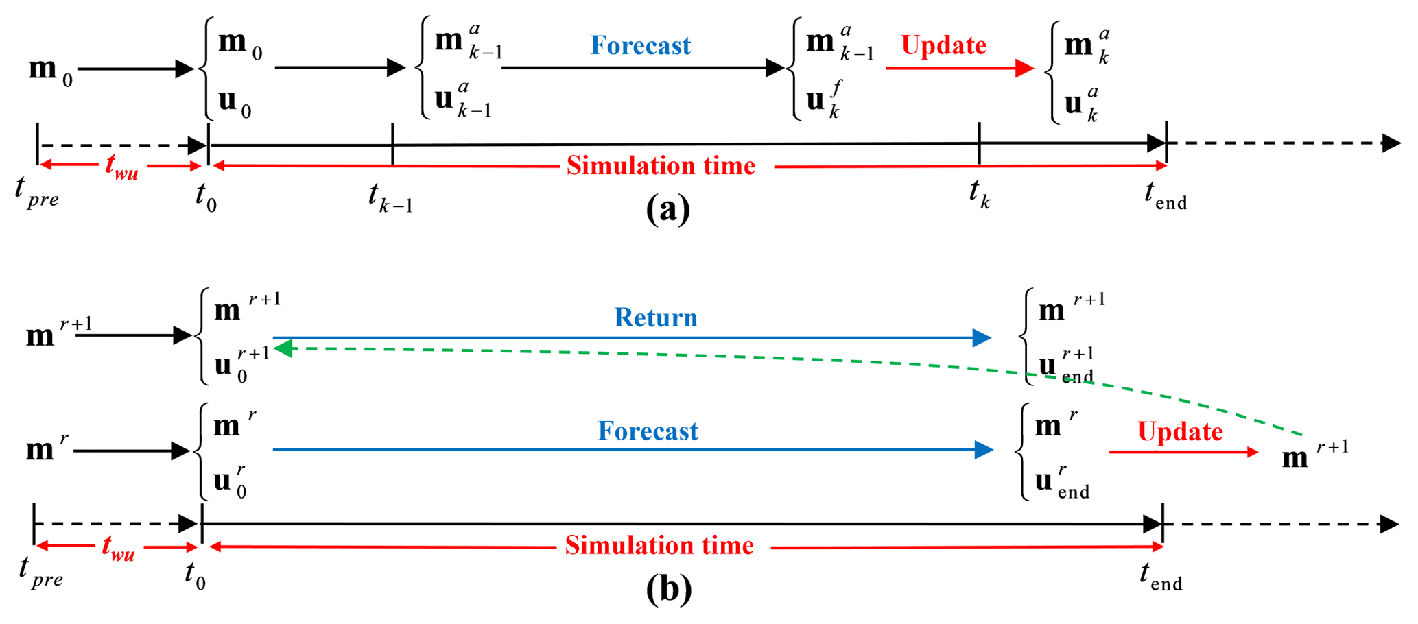
Figure 1Flow charts of simulation period – or data assimilation period with (a) ensemble Kalman filter (EnKF) and (b) iterative ensemble smoother (IES) – and warm-up period. t0 is the initial time, and tend is the end of simulation time. mk and uk are the vectors of model parameters (e.g., hydraulic conductivity) and state variables (e.g., soil moisture), respectively, at time tk, while mr and ur are the vectors at iteration r; the superscripts “a” and “f” refer to model analysis and forecast (or initial guess). Besides this, the period between tpre and t0 donates the process of warming up, and twu is the required warm-up time.
The EnKF approach was first proposed by Evensen (1994) and has been widely used in variably saturated flow problems (Huang et al., 2008; De Lannoy et al., 2007). This approach is a sequential data assimilation method (as shown in Fig. 1a) which incorporates observations into the model in order.
In this part, we assume that hydraulic parameters Ks, α and n are unknown, while the other parameters θr and θs are deterministic. The vector of the parameter and state is described as
where mk is the parameter vector (i.e., Ks, α and n), uk is state variables (i.e., soil moisture) at time tk, the dimension of yk is Ny: , where Nm indicates the amount of the parameters to be estimated, and Nd is the number of nodes of the numerical model. The updated soil moisture ensemble can be converted to the pressure head to drive the model. The observation vector can be defined as
where dk denotes the observations at time tk, εj,k values (j=1, 2, …, Ne) are independent Gaussian noises added to the observations and dj,k is the observation vector for ensemble index j at time tk. Based on the differences of model forecast and observations, the state–parameter vector can be updated to
where denotes the estimated or initially guessed values of parameter and state, while is the updated estimates, and H is an observation operator, linking the relationship between the state–parameter vector and the observation vector. K represents the Kalman gain matrix, which can be calculated as
where indicates the covariance matrix of observed data errors, while is the error covariance matrix of forecast ensemble, given by
where is the ensemble mean of .
Compared to EnKF, the IES gives a better estimate by taking all the available observations into consideration (van Leeuwen and Evensen, 1996), as presented in Fig. 1b. Thus, it can keep the overall consistency of parameters and state variables over time effectively and has been increasingly used to solve the parameter estimation problem in hydrology (Crestani et al., 2013; Emerick and Reynolds, 2013). By calculating iteratively, the nonlinear relationship between observation and parameter is linearized and the information content of the observations can be fully utilized (Chen and Oliver, 2013). In this case, we write the analyzed vector of model parameters as
The notation is similar to the one presented for EnKF, where “r” is the iteration index, is the initially guessed or estimated parameters for realization j at iteration r, and is the updated estimates for realization j by conditioning on the observed information at iteration r. It should be noted that the and denote the total number of observations and predicted data at iteration r, which is different from EnKF. The Kalman gain K is defined as
where is the cross-covariance matrix between the prior vector of model and the vector of predicted data at iteration r, is the auto-covariance matrix of predicted data at iteration r, and CD is the covariance matrix of observed data errors. λ donates a dynamic stability multiplier, which is set as 10 initially and can be adjusted adaptively according to the data misfit at every iteration; diag() is a diagonal matrix with the same diagonal elements as . Mathematically, the dynamic stabilizer term facilitates the solution switching between the Gauss–Newton solution and the steepest-descent method, which is known as the Levenberg–Marquardt approach (Pujol, 2007).
2.2.3 Quantitative index for data assimilation
To assess model parameter and state estimations, the root-mean-square error (RMSE) of estimated parameters (RMSEm) and soil moisture (RMSEobs) and the relative error index (RE) are computed as follows:
where represents the estimated parameter of realization j at the last simulation day (EnKF) or the last iteration (IES) and mT represents the true parameter listed in Table 1. and indicate the predicted and measured soil moisture, respectively. Nobs is the amount of observations. RMSE and RMSE represent the RMSE of the estimated and prior parameters, respectively. RE varies from 0 to positive infinity. As RE approaches 0, the analysis result is close to the truth, but a large value of RE (more than 1) indicates a bad parameter estimation. Compared with the RMSEm, this index can better present the improvement of parameter estimation during data assimilation.

A series of synthetic numerical experiments are performed in this section. In Sect. 3.1, we give a general description of the numerical experiments. In order to gain a better understanding of the propagation of the UIC, all the hydraulic parameters (i.e., Ks, α and n) are deterministic, and the UIC is the only uncertainty source in Sect. 3.2. Finally, the numerical cases are designed to evaluate performances of data assimilation algorithms combined with various initialization methods in Sect. 3.3, in which the parameter uncertainty is taken into consideration in conjunction with the UIC.
3.1 General description of model inputs
As shown in Table 1, four soils (sand, loam, silt and clay loam) are chosen in this study to explore the impacts of soil hydraulic property on the UIC. The values of hydraulic parameters are determined according to Carsel and Parrish (1988). Besides this, the effects of the meteorological condition are also considered: M-AC, M-SC and M-HC in Fig. 2 represent three sets of precipitation and potential evaporation data from three different regions (arid region, semi-arid region and humid region) in China.
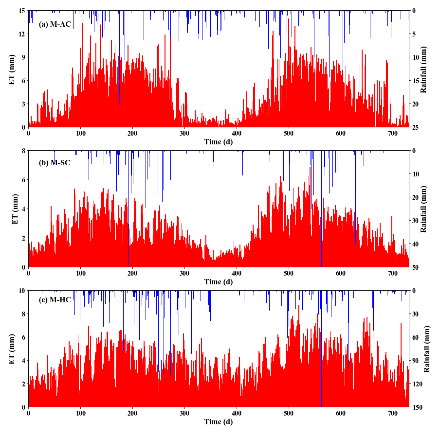
Figure 2Synthetic rainfall (blue bars) and potential evaporation (red bars) of three typical climates: (a) arid climate, (b) semi-arid climate and (c) humid climate. It should be noted that the meteorological data of simulation period are from day 366 to day 730.
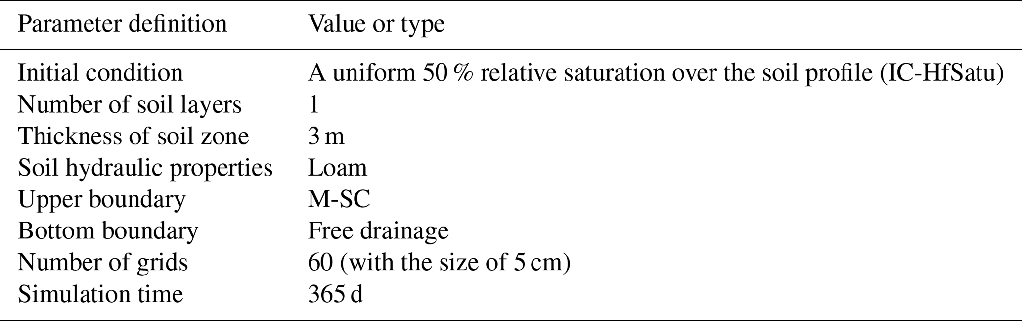
Unless otherwise specified, a uniform soil profile with the 50 % relative saturation (a value of 0.254 for loam) is chosen as the initial condition (IC-HfSatu). The soil profile is set to be 300 cm thick and is filled with loam. The flow domain is discretized into 60 grids with a grid size of 5 cm, which has been proved to be sufficient for evaluating the UIC in our study (results not shown). Besides this, the total simulation time during the synthetic simulation is 1 year (365 d). In addition, the default upper and bottom boundaries are set to be M-SC and the free drainage boundary, respectively. Other specifications and assumptions for our model simulation runs are given in Table 2.
3.2 The temporal evolution of UIC
3.2.1 Comparison of UIC quantification methods
A synthetic experiment is conducted to compare two methods (i.e., spin-up method and Monte Carlo method) in quantifying the UIC. Using the spin-up method, the first case runs a single simulation for 10 years by repeating the preceding meteorological condition starting with IC-HfSatu (Fig. 3a), and the percentage cutoff PC is calculated. In the second case, the Gaussian noise with a standard deviation of 3 % (determined according to the observation error of soil moisture) is added to the IC-HfSatu to generate an ensemble with different initial soil moisture profiles. Then we run different model realizations (Fig. 3b). Finally, the PC and Spvalues of the two cases versus time are compared in Fig. 3c.
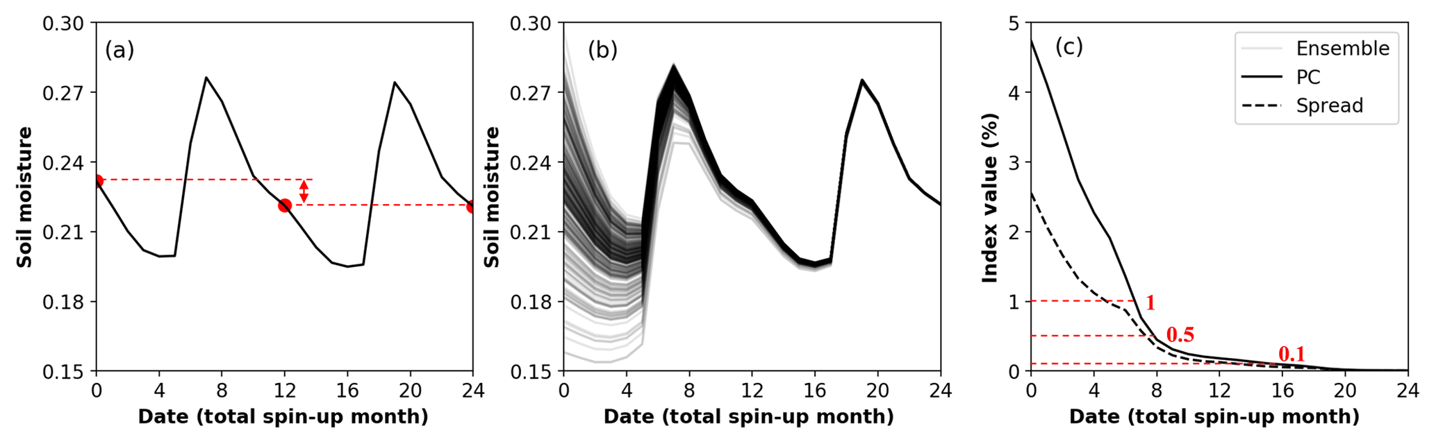
Figure 3Comparison of spin-up and Monte Carlo methods in determining warm-up time. (a) The spin-up method with monthly averaged soil moisture versus time by running a simulation recursively for 10 years, (b) Monte Carlo method with monthly averaged soil moisture of different realizations versus time based on various initial conditions, and (c) comparison of PC and Sp versus time. For the purpose of demonstration, the parameter uncertainty is not considered, and we only show the results of the first 2 years in the figure.
As shown in Fig. 3a, there is a visible difference between the monthly averaged soil moisture at the beginning and the 12th month, while the difference is much smaller for θ at the 12th and 24th months, indicating the decay of the UIC. Similarly, the soil moisture values from different realizations gradually get closer to each other. As shown in Fig. 3c, PC and Sp values gradually decrease with the simulation time, and their values are approximately the same after t>6 months. The significant difference at the beginning (PC of 4.7 % and Sp of 2.6 %) is due to different initial soil moisture values given by the spin-up and Monte Carlo methods. The result indicates that the widely used the spin-up method and Monte Carlo method are equivalent in terms of quantifying the UIC. We will use Monte Carlo method for the rest of the study, since it is consistent with the data assimilation approaches used in this study.
The determination of the threshold value when the UIC is regarded to have negligible effects on modeling has been discussed in previous studies (Ajami et al., 2014; Lim et al., 2012; Seck et al., 2014). PC or Sp values of 1 % (Yang et al., 1995), 0.1 % (De Goncalves et al., 2006) or 0.01 % (Henderson-Sellers et al., 1993) have been used. As shown in Fig. 3c, there is a significant diversity in the results between the spin-up and Monte Carlo methods at the index value of 1 %, indicating that the UIC still plays a significant role. In contrast, the requested twu is more than 15 months for a value of 0.1 %. To balance the estimation accuracy and computational cost, we recommend a threshold of 0.5 % for both the spin-up and Monte Carlo methods; the corresponding warm-up time twu is 8 months, which is long enough for the UIC to diminish, and the difference between PC and Sp is insignificant.
3.2.2 The influencing factors on UIC
The Monte Carlo method is used in this part to obtain the warm-up time twu, and a number of scenarios are constructed under a variety of conditions (different soils, meteorological conditions and soil profile lengths). First, the influence of soil texture and the meteorological condition on twu are examined. Four different types of homogeneous soils (sand, loam, silt and clay loam listed in Table 1) and a heterogeneous soil with multiple layers – consisting of loam (0–75 cm), clay loam (75–150 cm), silt (150–225 cm) and sand (225–300 cm) – under three typical meteorological conditions (M-AC, M-SC and M-HC) are employed in these scenarios, while the other model inputs use the default values (see Table 2). Besides this, the influence of different soil profile lengths (1, 3, 5, 10, 15 and 20 m) on the UIC is also investigated.
a. The influences of soil texture and meteorological condition
Figure 4 plots twu with five different soils under three typical meteorological conditions. The computational times vary greatly according to soil property. We find that twu values of sand are all less than 1 d, whereas twu values of loam are 412, 242 and 195 d. In addition, the warm-up times of silt and clay loam with M-AC and M-SC exceed 10 years, while those with M-HC are 264 and 253 d. The results imply that the warm-up time twu for the fine-textured soil is larger than that for coarse-textured soil. This may be attributed to the diversity of the drainage property for different soils. For sand, due to its fast drainage property, the soil moisture ensemble converges extremely quickly and most of the values at the profile are maintained as residual soil moisture. Thus, the UIC of sand disappears very quickly. In contrast, the soil moisture states for silt and clay loam change more slowly than sand during the simulation. Therefore, the faster drainage property leads to a smaller warm-up time.

Figure 4The length of warm-up time twu with various soils and meteorological conditions. Note that some of the twu values are larger than 10 years and are not able to be obtained due to the 10-year simulation time. The heterogeneous soil profile consists of loam (0–75 cm), clay loam (75–150 cm), silt (150–225 cm) and sand (225–300 cm).
In addition, the meteorological condition has a strong impact on the UIC. For example, with soil loam, the order of twu is M-HC < M-SC < M-AC. For silt and clay loam, twu values of M-AC and M-SC decrease from more than 10 years to 264 and 253 d with a humid climate M-HC, respectively. With intensive and excessive rainfall events, θ approaches the saturated soil moisture, leading to a sudden drop in Sp. Thus, the meteorological condition, especially the precipitation, plays an important role in the propagation of the UIC. Moreover, regarding the heterogeneous soil with multiple layers, the twu under the M-AC is larger than 10 years (similar to silt and clay loam), while that under M-SC or M-HC becomes much smaller (higher than that of loam, but they are of the same magnitude). Thus, it is conjectured that twu is determined by the fine soil texture in the layered profile under the dry meteorological condition but averaged soil hydraulic properties under the wet meteorological condition.
It should be noted that the twu is also relevant to the initial state of soil. Regarding the initial condition in an extremely dry state under the arid climate, the hydraulic conductivity is very small and the initial spread extends for a long time. For instance, twu of sand increases from 1 to 8 d when the ensemble mean value of initial soil moisture decreases from 0.2375 to 0.15 (results not shown). Yet, if a sufficiently large rain event takes place, the soil moisture increases and then converges to a similar state rapidly.
b. The influence of soil profile length
To investigate the effects of soil profile length on warm-up time, we investigate the twu values for simulations with various soil profile lengths. As presented in Fig. 5a, the twu values for soil lengths of 1, 3, 5, 10, 15 and 20 m are 0.11, 0.57, 0.74, 1.57, 2.78 and 4.3 years, respectively, indicating that the warm-up time increases with increasing depth of soil column. Figure 5b plots the twu value for each depth with the profile length of 20 m, showing that a longer warm-up time is needed if the soil layer is deeper. Both subfigures imply that the UIC decays more slowly if the effects of the boundary condition become less important. We also examine the case for substituting the free drainage boundary for a prescribed groundwater table. The results indicate that the twu is further shortened due to the influence of the bottom saturation condition (not shown).
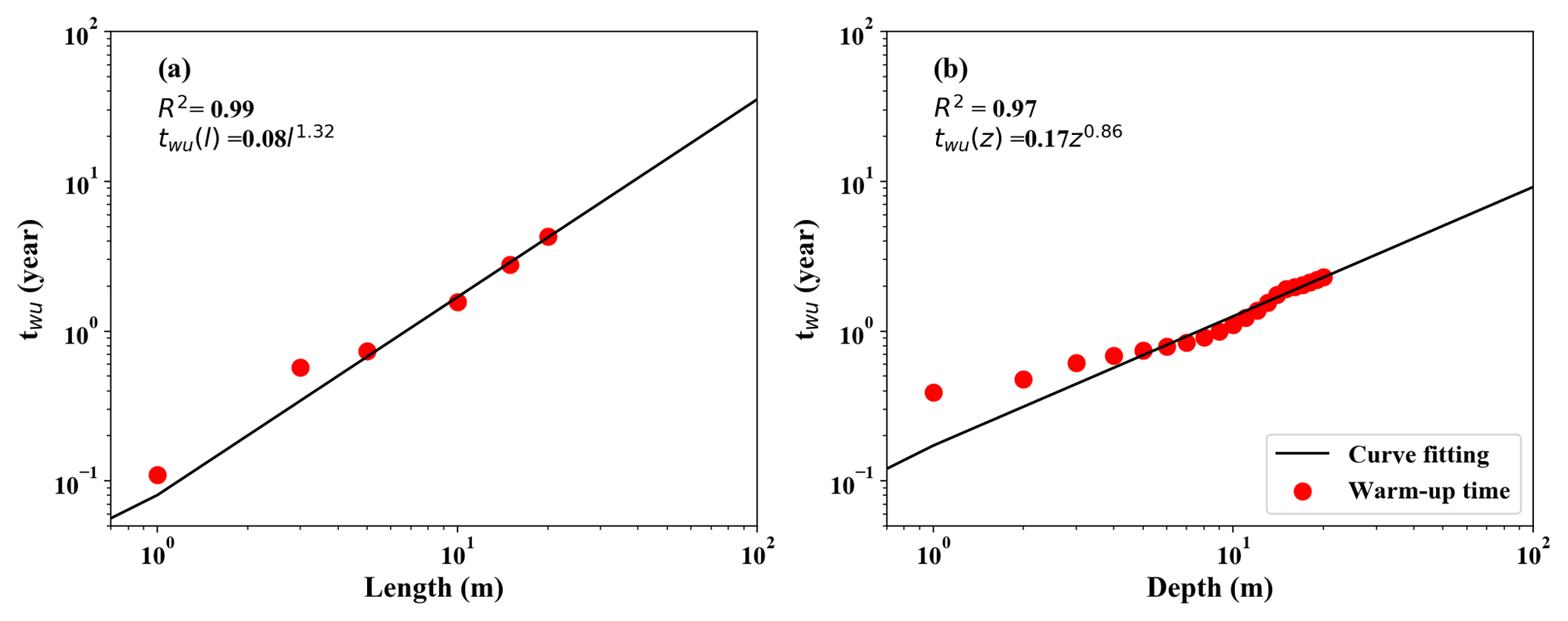
Figure 5The value of the warm-up time twu. (a) The overall profile twu values versus different soil profile lengths (l), and (b) twu value as a function of depth z with a 20 m soil profile.
In addition, twu in homogeneous loam reveals a power-law relationship with the length of soil profile. According to the fitted curve in Fig. 5a, the warm-up time twu is more than 7 years for a depth d of 30 m (e.g., North China Plain; Huo et al., 2014) and 700 years for d=1000 m (e.g., Yucca Mountain site; Flint et al., 2001) with loam soil. This result suggests that we should be very careful in dealing with a simulation with a long unsaturated profile where the UIC lasts for an extremely long time and influences the simulation and data assimilation results.
3.3 Initialization of data assimilation
Besides IC-HfSatu, two other common methods to prescribe initial conditions in variably saturated flow model based on the availability of information are also considered in this study, including a linear interpolation between observations (at depths of 10, 80, 150, 220 and 290 cm) at the beginning of simulation (IC-ObsInt) and a steady-state soil moisture profile by warming up the model with a constant infiltration flux of 1 mm d−1 (IC-flux). Moreover, we employ two warm-up methods, which give initial conditions by running the model prior to the beginning of simulation period with available meteorological data (as shown in Fig. 2). If the preceding meteorological data before the simulation period are available, they are used in the warm-up method (IC-WUP); otherwise, we use the meteorological data at the experimental period as a surrogate (IC-WUE). The length of warm-up time for IC-flux, IC-WUP and IC-WUE is equal to twu (242 d) based on the results in Sect. 3.2.2a, so the warm-up period of these three methods is from day 124 to day 365. In addition, IC-HfSatu and IC-ObsInt are assumed to be deterministic without uncertainty, while for the IC-flux, IC-WUP and IC-WUE, the uncertainty of states is introduced by warming up the model with uncertain parameters.
Thus, a total of five initialization methods (IC-HfSatu, IC-ObsInt, IC-NetFlux, IC-WUP and IC-WUE) are assessed to investigate the effect of the UIC on model state and parameter estimations within two data assimilation frameworks (EnKF and IES). The initial realizations of soil hydraulic parameters Ks, α and n for all data assimilation models are generated following logarithm-normal distributions, with mean values of 4.7 m d−1, 8.6 m−1 and 1.8 and variances (log transformed) of 0.1, 0.3 and 0.006. The saturated soil moisture θs and residual soil moisture θr are assumed to be deterministic with the value of 0.43 and 0.078. Compared with the reference values (Ks, α and n for loam are 0.2496 m d−1, 3.6 m−1 and 1.56, respectively) listed in Table 1, the prior means of unknown parameters are biased.
3.3.1 General description for various data assimilation cases
Several test cases are conducted to explore the effects of initialization on parameter estimation under various data assimilation frameworks. Case 1 investigates the effects of five initialization methods on individual parameter estimation with EnKF and the IES, respectively. Then, we increase the ensemble size of IC-HfSatu and IC-ObsInt to 500 (hereafter referred to as IC-HfSatu-500 and IC-ObsInt-500) in Case 2 to demonstrate the impacts of ensemble size. Case 3 explores the effects of the uncertainty magnitude of the initial ensemble on the parameter estimations. A Gaussian noise with a standard deviation of 0.017 (counted from IC-WUP) is added to both IC-HfSatu-500 and IC-ObsInt-500 (hereafter referred to as IC-HfSatu-500-Un and IC-ObsInt-500-Un). Furthermore, to find out the role of the initial condition in multi-parameter inverse problems, Case 4 is conducted to estimate Ks, α and n simultaneously. Case 5 is implemented with a simulation time of 60 d to explore the influence of assimilation time on multiple parameter estimation with the IES. It should be noted that the warm-up methods (IC-WUP and IC-WUE) are used in the IES warm-up model before every iteration (as presented in Fig. 1b), since the initialization of the IES by warming up the model for only the first iteration leads to poor assimilation results.
The synthetic observations used for data assimilation are generated by running the model with the true parameter (loam) and true initial condition (produced by warming up model with a sufficient long time of 10 years). The generated observations are perturbed by a Gaussian noise with a standard deviation of 0.01. A total number of 37 observations are assimilated into the model. The observation depth is at z=10 cm, and the observed soil moisture is assimilated every 10 d, starting from day 3. The details of the model inputs for Case 1 to Case 5 are listed in Table 3.
Table 3Case summary for parameter estimation within EnKF and IES.
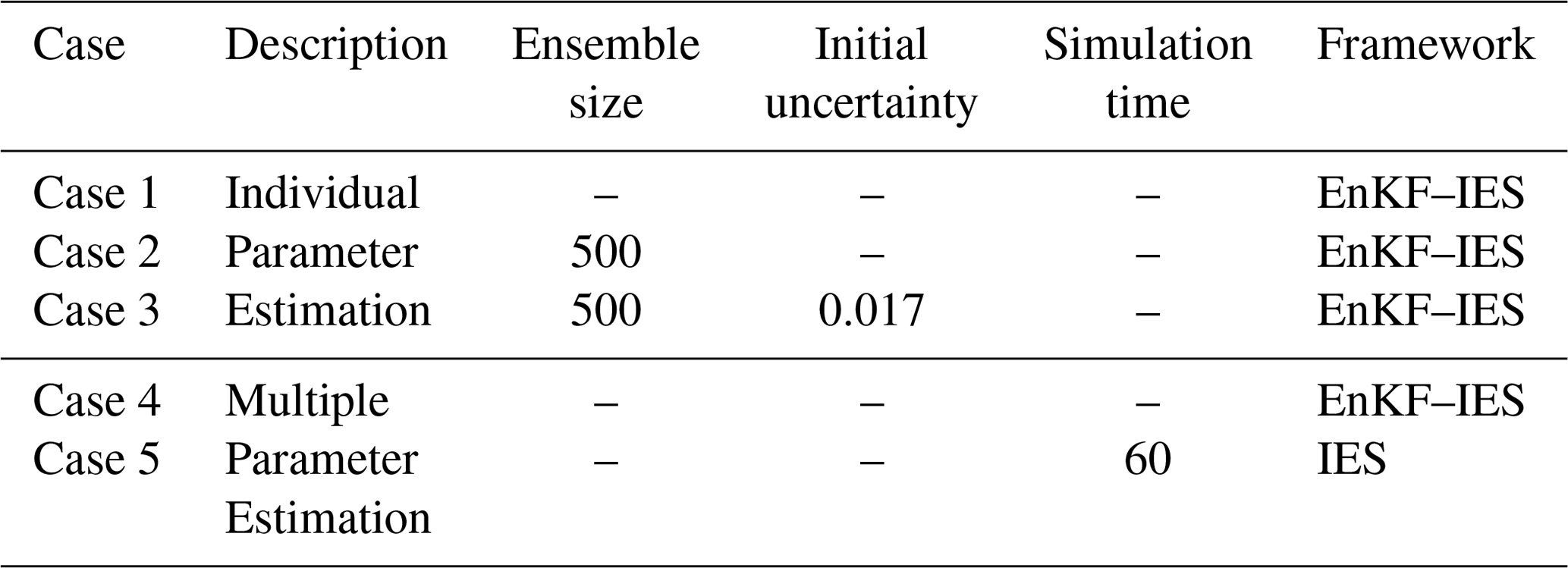
Note: values that are not given use the default values. The default value of initial uncertainty for IC-ObsInt and IC-HfSatu is 0.
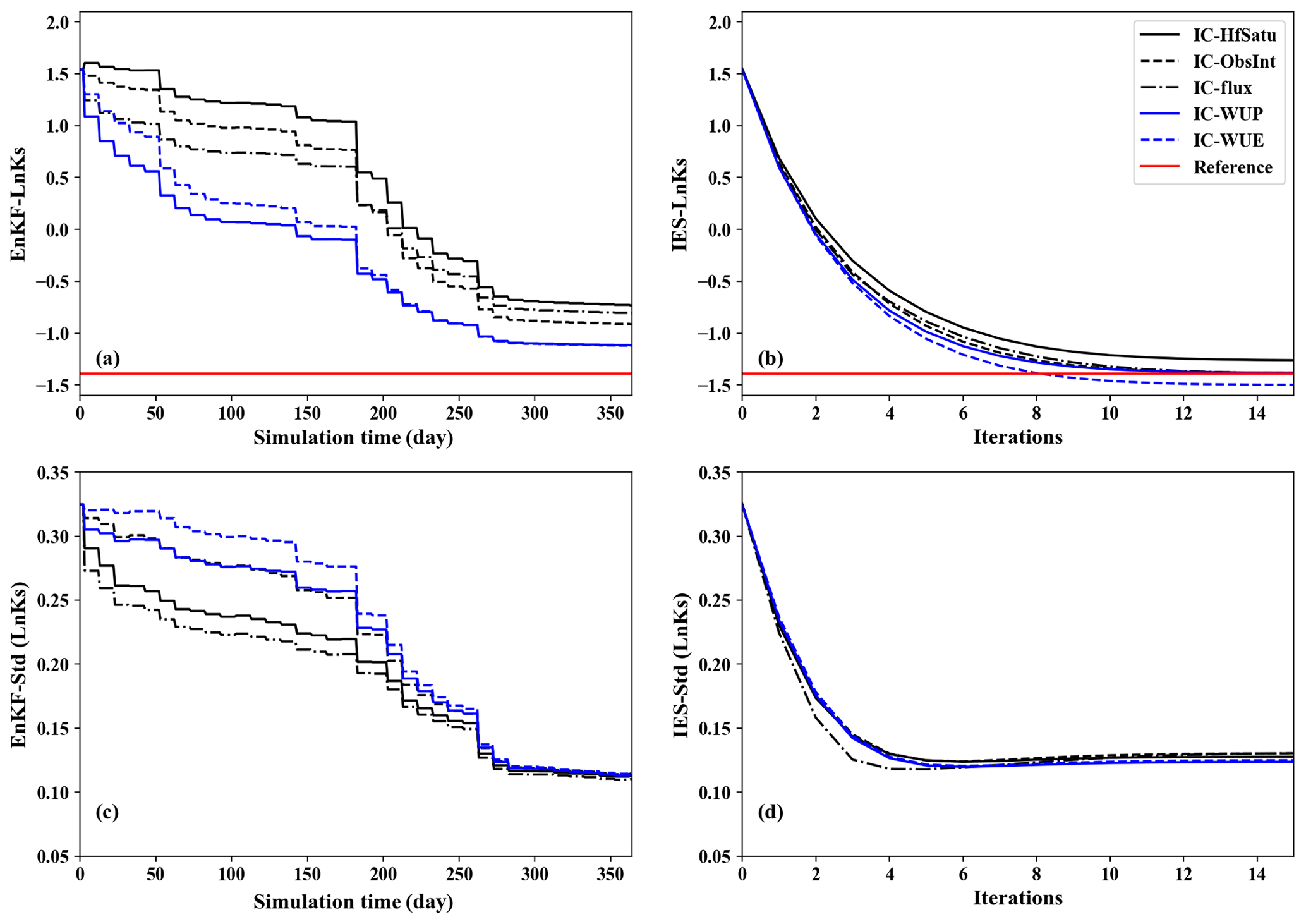
Figure 6The results of ln Ks estimations (a, b) and their associated standard deviations (c, d) within two data assimilation frameworks (a, c: EnKF; b, d: IES) under five initialization methods (Case 1).
3.3.2 Result
The results for parameter estimation (ln Ks) using the two data assimilation frameworks with different initialization methods (Case 1) are compared in Fig. 6. In Fig. 6a, the estimated ln Ks values of EnKF are presented. In general, the ln Ks estimations under different initial conditions all gradually approach the true values over assimilation time, but the final assimilation results are different. For IC-HfSatu, because the initial profile is uniform and arbitrarily specified, the assimilation results are affected by the parameter uncertainty and the UIC simultaneously. Thus, the decrease in RMSEm is the slowest, and the final parameter estimation result is the worst. In contrast, the initial conditions generated by warm-up methods (IC-WUP and IC-WUE) can eliminate the UIC in advance, and thus data assimilation can handle parameter uncertainty more efficiently, leading to the best results among the five. The data assimilation results of IC-WUE are a little worse than those of IC-WUP, owing to the diversity of the meteorological condition. Since IC-ObsInt and IC-flux are created by adding observation information or simple infiltration information, they perform better than that with IC-HfSatu but worse than warm-up methods. Similarly, the assimilation results for the IES with IC-WUP are also the best, while those with IC-HfSatu have the worst parameter estimation in the five initialization methods (Fig. 6b). In addition, by comparing Fig. 6a and b, the cases using the IES show better results than those using EnKF, indicating a superior ability of the IES to estimate the individual parameter in variably saturated model. However, since the IES estimates parameter iteratively, it has a much larger computational cost than EnKF when using warm-up methods.
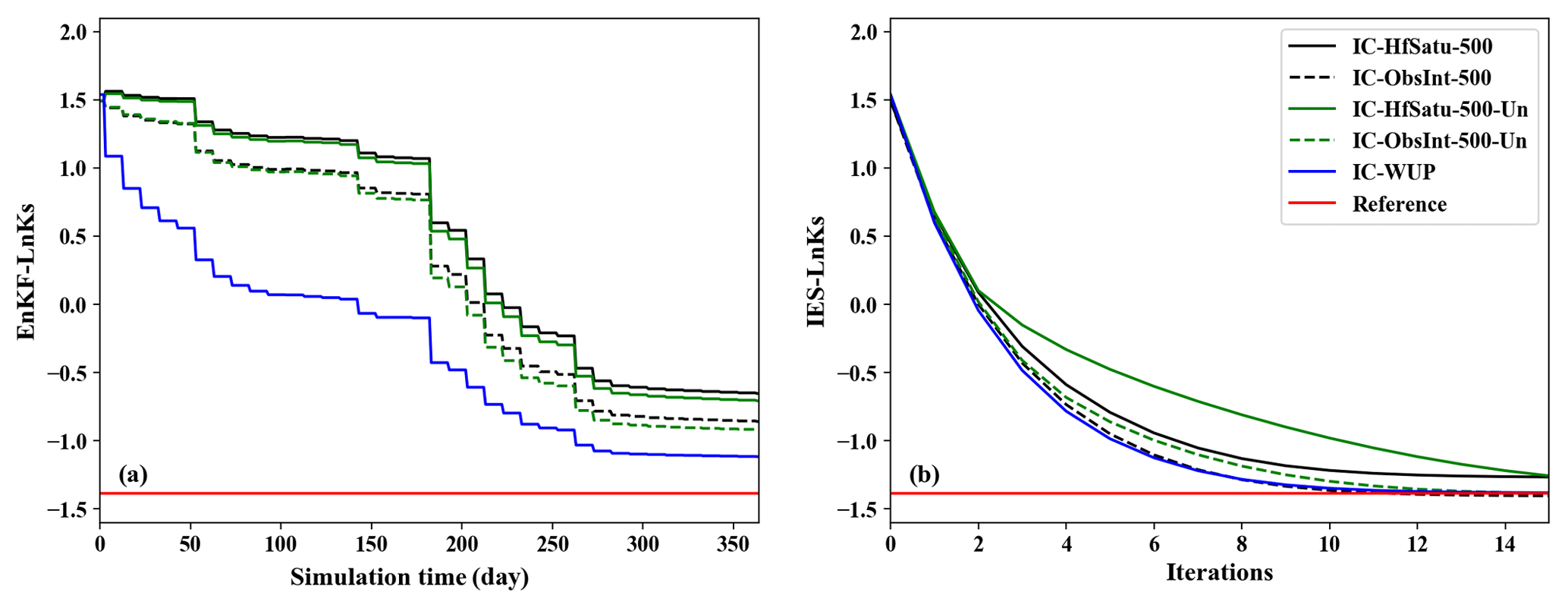
Figure 7The impacts of increased ensemble size (Case 2) and uncertainty of initial state (Case 3) on the results of ln Ks estimations within EnKF and IES.
For the data assimilation problem, the ensemble variance is increasingly underestimated over time and iteration, which may cause the filter inbreeding problem (Hendricks Franssen and Kinzelbach, 2008). To determine if our data assimilation runs are affected by filter inbreeding, the temporal change of the standard deviation of estimated ln Ks is plotted in Fig. 6c and d. In general, the standard deviation of estimated ln Ks declines gradually with assimilation steps (EnKF) or iteration steps (IES). As given in Fig. 6a and c, the filter inbreeding might take place after 280th days for EnKF, since the standard deviations of ensemble all approach 0.1 and the estimated parameters stay constant over time. However, with the help of a damping parameter, the filter inbreeding problem for the IES could be reduced significantly. This partly explains the inferior result of EnKF compared to the IES.
Increasing the ensemble size and model uncertainty is an efficient approach for reducing the filter inbreeding (Hendricks Franssen and Kinzelbach, 2008). To demonstrate the impacts of ensemble size and initial uncertainty on data assimilation results, the results of ln Ks estimations utilizing the initial condition IC-HfSatu and IC-ObsInt with the ensemble size of 500 (Case 2) and a Gaussian noise (Case 3) are plotted in the Fig. 7.
The results of IC-HfSatu-500 and IC-ObsInt-500 with the ensemble size of 500 in Fig. 7 are similar to those of IC-HfSatu and IC-ObsInt (Fig. 6), indicating that the improvement of the parameter estimation result is slight when the ensemble size increases from 300 to 500. Hence, the ensemble size of 300 is sufficient for the data assimilation problem in this study. In contrast, the influences of adding the uncertainty to the initial state on parameter estimation are totally different for EnKF and the IES. Compared with the results of IC-ObsInt-500 and IC-HfSatu-500, the results of ln Ks estimation with IC-ObsInt-500-Un and IC-HfSatu-500-Un improve for EnKF (Fig. 7a) but deteriorate for the IES (Fig. 7b). This may be attributed to the diversity between two algorithms. EnKF is a sequential algorithm, so the state uncertainty introduced by the UIC could decrease over assimilation steps. A larger ensemble state variance implemented at the beginning leads to a larger trust in data and thus a quicker update of the parameter to truth and can prevent EnKF from inbreeding, leading to a better result than that with an initial condition of small variance. On the contrary, the IES is a batch optimization method. The uncertainty of the initial state exists at each iteration and has a negative effect on the model calibration during the whole simulation, worsening the parameter estimation results. Besides this, we also investigate the influences of spatial correlation of the added noise (e.g., with correlation length of 50 cm or infinity) for constructing IC-HfSatu and IC-ObsInt, but their parameter estimation results are similar (not shown), indicating that the effects of spatial correlation of noise during the construction of IC-HfSatu and IC-ObsInt are not significant in parameter estimation.
Moreover, the parameter estimation results of IC-WUP are still superior to those of IC-HfSatu-500-Un and IC-ObsInt-500-Un even though they all have a similar computational cost, showing the promising performance of warm-up methods. The results are reasonable, since all ensemble Kalman filter methods are affected by the quality of the auto-covariance matrix and the mean value of the predicted state ensemble (Eqs. 11 and 12 for EnKF; Eqs. 14 and 15 for IES). For the WUP method, the initial condition is constructed by warming up the model with the prior parameter; thus IC-WUP contains useful information of prior parameter, even it is biased. Besides this, the state covariance matrix is implicitly inflated due to the introduction of uncertain prior parameter ensemble during warming up. These two aspects ensure the robust performance of warm-up methods. However, the initial state ensembles of IC-HfSatu-500-Un and IC-ObsInt-500-Un are independent of the prior parameter, which introduces additional uncertainties, making the data assimilation results worse. Therefore, even using a larger ensemble size and enlarging the state uncertainty (covariance inflation), warm-up methods are still the optimal choice for both EnKF and IES algorithms. We also construct another case with larger parameter uncertainty to alleviate the filter inbreeding problem, and the data assimilation for all cases are improved (not shown). The results also agree with our conclusion that WUP performs the best among the five initialization methods.
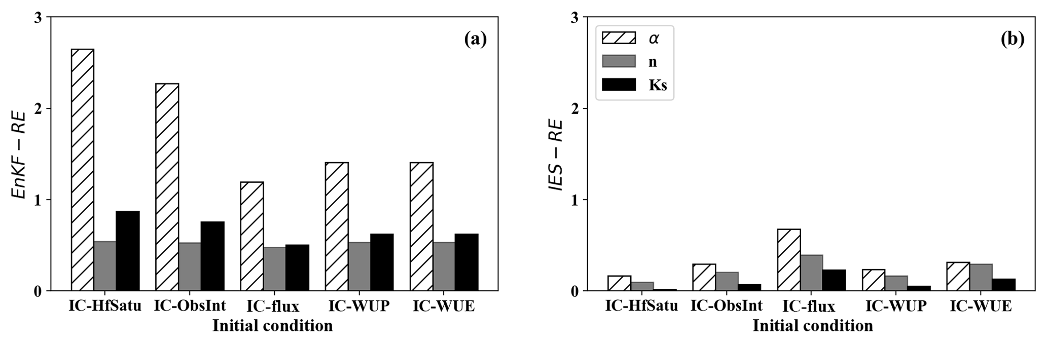
Figure 8The RE results of parameter estimations (α, n and Ks) under five initialization methods with (a) EnKF and (b) IES (Case 4).
To evaluate the effects of the UIC in the multi-parameter inverse problem, the RE results of Ks, α and n estimates of Case 4 are presented in Fig. 8. In general, the RE results of n and Ks are small no matter whether EnKF or the IES is used or not, while the RE of α is the largest. A cross-correlation analysis indicates that soil moisture observations are insensitive to parameter α with a free drainage boundary condition, which agrees with the results of Hu et al. (2017). In Fig. 8a, similar to the conclusion of the one-parameter inverse problem, the parameter estimation results of Ks and α with IC-HfSatu and IC-ObsInt are worse than those of IC-WUP and IC-WUE. There is not much difference between the n estimates under various initial conditions, implying that n is less affected by the UIC when estimating Ks, α and n simultaneously. Compared with EnKF, the IES shows a smaller RE (Fig. 8b) for all parameters, indicating that the IES can also perform better in the multi-parameter inverse problem. However, the assimilation results with various initialization methods do not show much difference, implying that the final RE values are not significantly affected by the UIC, possibly due to abundant observations available over 1 year. Nevertheless, long-term observation data may not be available in many cases.
To examine the impact of assimilation time on parameter estimation with the IES, Case 5 with a shorter assimilation period (60 d) and a fewer number of observations (i.e., six) is conducted. Figure 9 shows the RE results, and it is inferior to those in Case 4, where the simulation time is 1 year (Fig. 8b). Nevertheless, the effects of assimilation time on parameter estimation are different for different parameters. For instance, parameter n can still be estimated well in the most of the situations. In addition, though the assimilation results of Ks degraded with a 60 d simulation, the variation in Ks estimation values among different initialization methods is small. The number of observations can greatly affect the estimation of parameter α, since RE values of α in Case 5 (3.5, 4.8, 1.17, 0.79 and 0.23) are much larger than those in Case 4 (0.16, 0.29, 0.68, 0.24 and 0.31). Furthermore, the warm-up methods show the best data assimilation results among the five when the observations are insufficient.
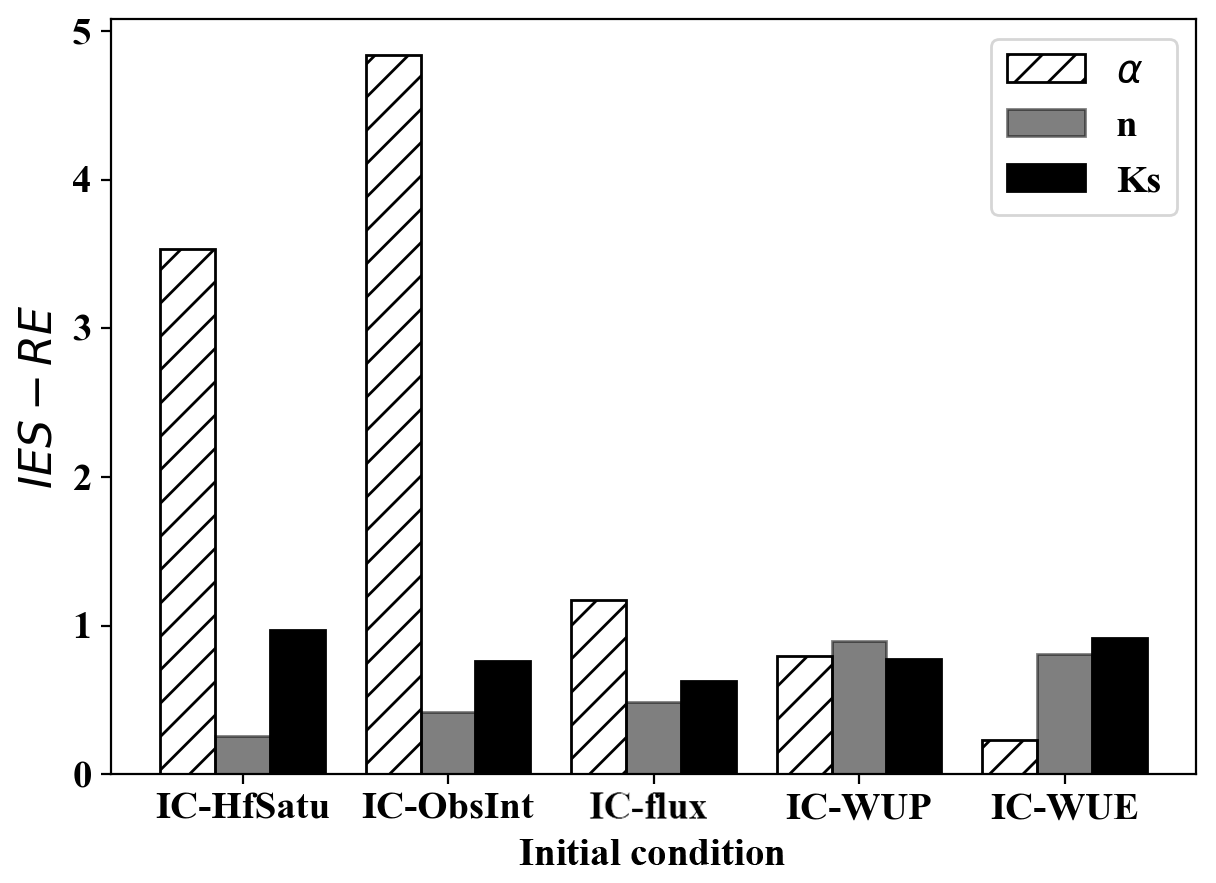
Figure 9The RE results of parameter estimations under five initialization methods with IES when the simulation time is 60 d (Case 5).
Synthetic observation in previous section is generated by running the model with uncertainty sources that are exactly known. By conducting synthetic experiments, we can thoroughly analyze the impact of the UIC during data assimilation, with scenarios having different numbers of observations and/or unknown parameters, and more decisive conclusions can be drawn. In contrast, the field observations contain additional uncertainties which are largely unknown (e.g., the calculated evapotranspiration is inaccurate for the real-world case). In order to examine the real-world applicability of the conclusions drawn from synthetic case, field data are necessary for validating our results. A field experiment is conducted in the irrigation-drainage experimental site of Wuhan University (Li et al., 2018; Fig. 10a). Meteorological data, including air temperature, relative humidity, atmospheric pressure, incident solar radiation and precipitation, are continuously monitored by an automatic weather station (LoggerNet 4.0), which can be used as an upper boundary condition after the calculation of the potential evaporation (Penman–Monteith's equation) on the bare soil (see Fig. 11a). A vertically inserted frequency domain reflectometry (FDR) tube was used to monitor soil moisture (Fig. 10b). The in situ soil moisture observation was measured every 3 d. The tube gave soil moisture measurements at the depths of 10, 20 and 30 cm. During 18 April to 30 May 2017, the measurements were repeated 14 times and 42 soil moisture data were collected (see Fig. 11b). Besides this, the soil moisture at the depths of 10, 20, 30, 40, 60 and 80 cm at the beginning of the simulation time is also available to construct an initial profile via IC-ObsInt.
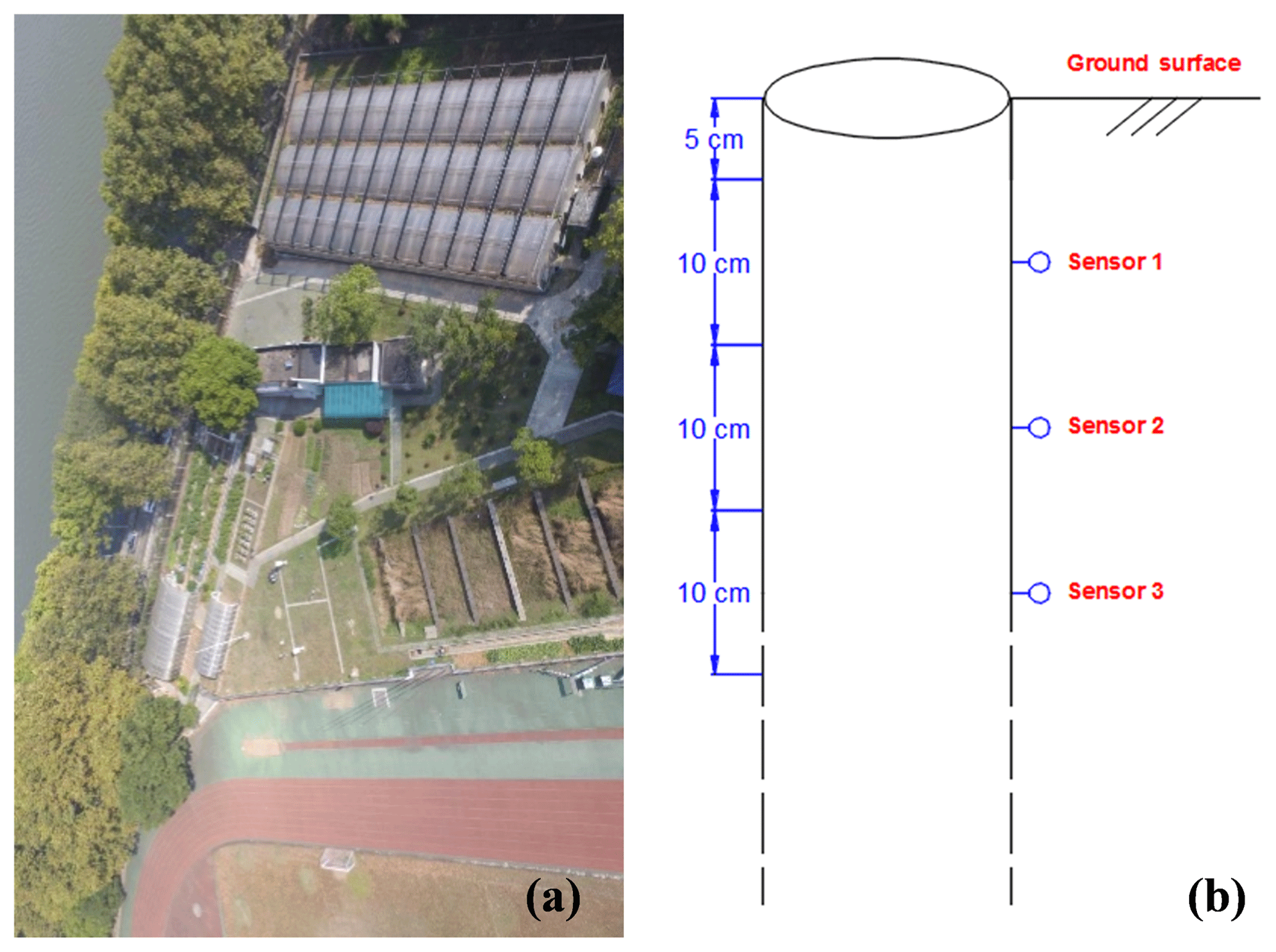
Figure 10The experimental site: (a) overhead view and (b) the cross-sectional view of the FDR sensor.
4.1 General description of the experimental case
To analyze the experimental data, the 1-D numerical domain is set as 2 m and discretized in 50 grids. The top 40 grids have a size of 2.5 cm, and the rest have a size of 10 cm. The upper boundary is set as an atmospheric boundary using the data shown in Fig. 11a, and the bottom boundary is set to be free drainage, since the groundwater table is much deeper than the bottom of the domain.
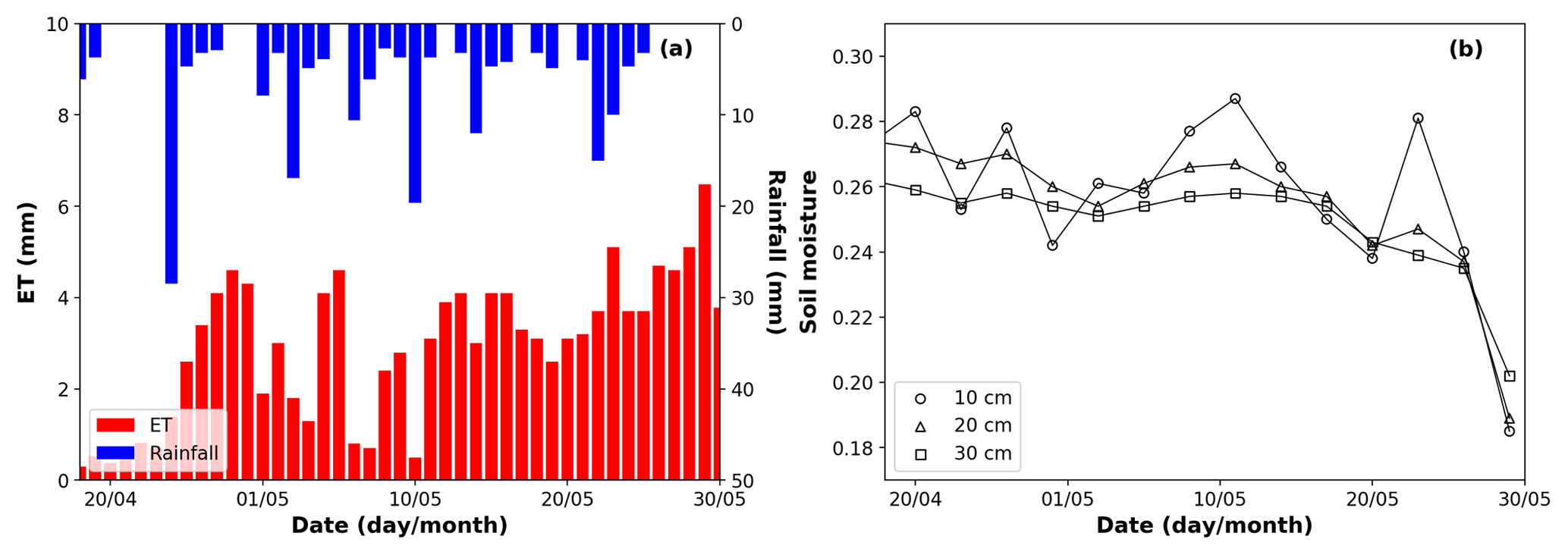
Figure 11The meteorological information and observed soil moisture over the experimental time. (a) Observed rainfall and calculated potential evaporation. (b) Temporal change of soil moisture data at three different observed depths (10, 20 and 30 cm).
The prior parameter distributions follow the study of Li et al. (2018). The saturated soil moisture θs and residual soil moisture θr are given as 0.43 and 0.078, while the other hydraulic parameters are to be estimated. The initial means of Ks, α and n are set as 1 m d−1, 5 m−1 and 2, and the initial natural logarithmic variances of them are set as 0.22, 0.16 and 0.003. The data from 18th April through 27 April are used for calibration, while the remaining data are reserved for validation. The climate of Wuhan is semi-arid conditions, and the soil of the experimental site is sandy loam. We use a warm-up time of 242 d based on our investigation in Sect. 3.2.2.
4.2 Results
The assimilation results with four different initialization results (IC-HfSatu, IC-ObsInt, IC-flux and IC-WUP) are presented in this part. Since the true hydraulic parameters at the experimental site are unknown, we assess the estimation by comparing the predicted (using estimated parameters) and observed soil moisture during the validation period. The RMSEobs values for soil moisture predictions under different assimilation scenarios are listed in Table 4. Generally speaking, RMSEobs values with IC-WUP are again the smallest, while IC-HfSatu has the largest RMSEobs values.
Table 4RMSEobs results for the soil moisture predictions at observation points with different initial conditions in the experimental case.

In order to evaluate the overall performances of the four initialization methods, the soil moisture observations and predictions at all depths are plotted in Fig. 12. The coefficients of determination under the four scenarios are 0.033, 0.599, 0.083 and 0.553, and the RMSEobs values are 0.045, 0.037, 0.036 and 0.028, respectively. As shown in Fig. 12a and c, IC-HfSatu and IC-flux show very large scattering, indicating a bad prediction performance. A significant improvement is found in IC-WUP, with a large R2 and the smallest RMSEobs value, as shown in Fig. 12d. Surprisingly, IC-ObsInt has the largest R2 among the four methods, though its RMSEobs value is bigger than that of IC-WUP. The simulation of real-world problems may have uncertainties that are not considered in data assimilation. For instance, the meteorological data prior to the simulation for warming up are not precise from the weather-station instrument error and calculation of evapotranspiration, which has a detrimental effect on IC-WUP. IC-ObsInt, on the other hand, has the advantage of utilizing the soil moisture observations for both initialization and predictions. However, IC-ObsInt may not be applicable when soil moisture observations at t=0 are not available or the soil moisture profile is discontinuous in layered soils, leading to a large interpolation error. In summary, for both the synthetic and field cases, models initialized using the warm-up method result in low uncertainty and superior soil moisture predictions even if the calibration data are insufficient.
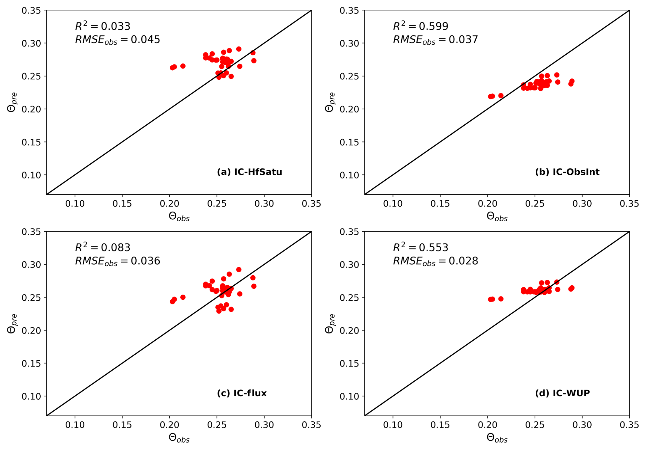
Figure 12The comparisons between soil moisture observations and predictions (with estimated parameters from IES combined with different initialization methods) at all observation depths.
The study investigates the effects of the UIC on variably saturated flow simulations subject to different soil hydraulic parameters, meteorological conditions and soil profile lengths. Two common approaches (spin-up and Monte Carlo methods) are applied to explore the required warm-up time twu and temporal behavior of the UIC. In addition, the data assimilation performances with five common initialization approaches are compared using synthetic experiments and a field soil moisture dataset.
Under the atmospheric boundary condition, the soil moisture value near the upper boundary could approach its upper and lower bounds (saturated water content and residual water content) due to rainfall and evaporation. This significantly reduces the UIC of soil moisture profile near the soil surface. Our investigation shows that the coarse-textured soil results in faster reduction of the soil moisture UIC because of fast redistribution of water in sandy soil. Regarding the influence of boundary conditions, we find that heavy rainfall can reduce the UIC significantly, while an initial condition in a drier status leads to a growth of twu, since a drier soil drains and evaporates less water, making the UIC of soil moisture dissipate slowly. The conclusion agrees with the conclusions reported by Castillo et al. (2003) and Seck et al. (2014). Although twu for sandy soil is very small, it could be very large for other soils (less than 1 d versus more than 10 years in Fig. 4). The length of soil profile plays an important role in the UIC, since the UIC decays from the boundaries. As a result, the UIC could exist persistently in a very thick vadose zone. Our findings imply that the UIC dissipation depends nonlinearly on the soil type, meteorological condition and soil profile lengths, and special attention should be paid during vadose zone modeling.
Ideally, the initial ensemble should represent the error statistics of the initial guess for the model state during data assimilation (Evensen, 2003). Thus, effort should be invested in reducing the impact of the UIC on data assimilation. Methods which do not consider the UIC (i.e., assuming an initial ensemble arbitrarily without uncertainty, which was used in some studies; e.g., Shi et al., 2015) can induce significant bias according to our data assimilation results. By constructing the initial condition using the information of observations or the boundary condition (averaged flux), the data assimilation results can be improved. However, these two initialization methods are also suboptimal due to the oversimplification of the complex initial condition. By warming up the model with available meteorological data, the initialization methods can improve data assimilation results. Moreover, EnKF is more sensitive to the filter inbreeding problem than the IES. The initial condition with a larger state uncertainty gains better performance than that without covariance inflation for EnKF, while for the IES, this inflated uncertainty cannot decrease over iterations, making the results inferior.
In this study, we only use the soil moisture observations rather than the pressure head to construct the initial profile. For homogeneous soil column, there is a one-to-one relationship between the spread of soil moisture and the pressure head (i.e., UIC in terms of the pressure head can be converted from that of soil moisture). The situation will be much more complex if the soil is heterogeneous, since a large number of unknown hydraulic parameters may introduce significant nonlinearity during the transformation between the head and soil moisture. For instance, the soil moisture profile is discontinuous in layered soils. The use of the pressure head instead of soil moisture as the initial condition for heterogeneous soils deserves investigation in our future work.
Our work leads to the following major conclusions:
-
The spin-up method and Monte Carlo method can both quantify the UIC, and they agree well with each other after a sufficiently long simulation. A threshold of 0.5 % for percentage cutoff PC or ensemble spread Sp is recommended to determine the warm-up time.
-
Warm-up time varies nonlinearly with soil textures, meteorological conditions and soil profile length. Under most situations (e.g., loam with the soil profile length less than 5 m under non-arid climate), a 1-year warm-up time is sufficient for soil water movement modeling, but an extremely long time (exceeds 10 years) is needed to warm up the model for a long, fine-textured soil profile under an arid meteorological condition.
-
The IES shows better performance than EnKF in the strongly nonlinear problem and is affected less by the UIC with a long period of observations. In addition, covariance inflation of the initial condition could improve the data assimilation results for EnKF but deteriorate them for the IES.
-
The following procedure is recommended to initialize soil water modeling: (1) evaluate the approximate warm-up time based on the model settings, (2) initialize the model using the method of the WUP (if meteorological data are available) and make sure the warm-up time is larger than the required twu, and (3) run the simulation with the initial condition obtained in step 2. WUE is an alternative to WUP if the preceding meteorological data are not available. ObsInt is also a practical choice if dense soil moisture observations at the beginning of simulation are available.
Further research may examine the performance of these initialization methods in two- or three-dimensional variably saturated flow conditions. Our approach can also be extended to other modeling and data assimilation problems in other disciplines (e.g., groundwater flow and solute transport modeling and soil–water–crop modeling).
All the data used in this study can be requested by email to the corresponding author Yuanyuan Zha at zhayuan87@gmail.com.
YZ and JY developed the new package for soil water flow modeling based switching the primary variable of the numerical Richards' equation; DY and YZ developed EnKF and the IES codes for data assimilation of variably saturated flow and designed and conducted the numerical cases and field data validation for this study. Seven of the co-authors made non-negligible efforts in preparing the paper.
The authors declare that they have no conflict of interest.
This work is supported by the Natural Science Foundation of China through grant nos. 51609173, 51779179 and 51861125202. The authors appreciate Michael Tso (Lancaster University, UK) for editing the paper. We thank the three reviewers for their constructive comments and suggestions.
This research has been supported by the National Natural Science Foundation of China (grant nos. 51609173, 51779179 and 51861125202).
This paper was edited by Bill X. Hu and reviewed by Heng Dai and two anonymous referees.
Ajami, H., McCabe, M. F., Evans, J. P., and Stisen, S: Assessing the impact of model warm-up on surface water-groundwater interactions using an integrated hydrologic model, Water Resour. Res., 50, 1–21, https://doi.org/10.1002/2013WR014258, 2014.
Ataie-Ashtiani, B., Volker, R. E., and Lockington, D. A.: Numerical and experimental study of seepage in unconfined aquifers with a periodic boundary condition, J. Hydrol., 222, 165–184, https://doi.org/10.1016/S0022-1694(99)00105-5, 1999.
Bauser, H. H., Jaumann, S., Berg, D., and Roth, K.: EnKF with closed-eye period – Towards a consistent aggregation of information in soil hydrology, Hydrol. Earth Syst. Sci., 20, 4999–5014, https://doi.org/10.5194/hess-20-4999-2016, 2016.
Carsel, R. F. and Parrish, R. S.: Developing joint probability distributions of soil water retention characteristics, Water Resour. Res., 24, 755–769, https://doi.org/10.1029/WR024i005p00755, 1988.
Castillo, V. M., Gómez-Plaza, A., and Martínez-Mena, M.: The role of antecedent soil water content in the runoff response of semiarid catchments:A simulation approach, J. Hydrol., 284, 114–130, https://doi.org/10.1016/S0022-1694(03)00264-6, 2003.
Chanzy, A., Mumen, M., and Richard, G.: Accuracy of top soil moisture simulation using a mechanistic model with limited soil characterization, Water Resour. Res., 44, 1–16, https://doi.org/10.1029/2006WR005765, 2008.
Chen, Y. and Oliver, D. S.: Levenberg-Marquardt forms of the iterative ensemble smoother for efficient history matching and uncertainty quantification, Comput. Geosci., 17, 689–703, https://doi.org/10.1007/s10596-013-9351-5, 2013.
Chirico, G. B., Medina, H., and Romano, N.: Kalman filters for assimilating near-surface observations into the Richards equation – Part 1: Retrieving state profiles with linear and nonlinear numerical schemes, Hydrol. Earth Syst. Sci., 18, 2503–2520, https://doi.org/10.5194/hess-18-2503-2014, 2014.
Cosgrove, B. A., Lohmann, D., Mitchell, K. E., Houser, P. R., Wood, E. F., Schaake, J. C., Robock, A., Sheffield, J., Duan, Q. Y., Luo, L. F., Higgins, R. W., Pinker, R. T., and Tarpley, J. D.: Land surface model spin-up behavior in the North American Land Data Assimilation System (NLDAS), J. Geophys. Res., 108, 8845, https://doi.org/10.1029/2002JD003316, 2003.
Crestani, E., Camporese, M., Baú, D., and Salandin, P.: Ensemble Kalman filter versus ensemble smoother for assessing hydraulic conductivity via tracer test data assimilation, Hydrol. Earth Syst. Sci., 17, 1517–1531, https://doi.org/10.5194/hess-17-1517-2013, 2013.
Das, N. N. and Mohanty, B. P.: Root zone soil moisture assessment using remote sensing and vadose zone modeling, Vadose Zone J., 5, 296, https://doi.org/10.2136/vzj2005.0033, 2006.
DeChant, C. M.: Quantifying the impacts of initial condition and model uncertainty on hydrological forecasts, PhD thesis, Portland State University, Portland, USA, 2014.
DeChant, C. M. and Moradkhani, H.: Improving the characterization of initial condition for ensemble streamflow prediction using data assimilation, Hydrol. Earth Syst. Sci., 15, 3399–3410, https://doi.org/10.5194/hess-15-3399-2011, 2011.
De Goncalves, L. G. G., Shuttleworth, W. J., Burke, E. J., Houser, P., Toll, D. L., Rodell, M., and Arsenault, K.: Toward a South America Land Data Assimilation System: Aspects of land surface model warm-up using the Simplified Simple Biosphere, J. Geophys. Res.-Atmos., 111, 1–13, https://doi.org/10.1029/2005JD006297, 2006.
De Lannoy, G. J., Reichle, R. H., Houser, P. R., Pauwels, V., and Verhoest, N. E.: Correcting for forecast bias in soil moisture assimilation with the ensemble Kalman filter. Water Resour. Res., 43, W09410, https://doi.org/10.1029/2006WR005449, 2007.
Doussan, C., Jouniaux, L., and Thony, J. L.: Variations of self-potential and unsatureated water flow with time in sandy loam and clay loam soils, J. Hydrol., 267, 173–185, https://doi.org/10.1016/S0022-1694(02)00148-8, 2002.
Emerick, A. A. and Reynolds, A. C.: Ensemble smoother with multiple data assimilation, Comput. Geosci., 55, 3–15, https://doi.org/10.1016/j.cageo.2012.03.011, 2013.
Erdal, D., Neuweiler, I., and Wollschläger, U.: Using a bias aware EnKF to account for unresolved structure in an unsaturated zone model, Water Resour. Res., 50, 132–147, https://doi.org/10.1002/2012WR013443, 2014.
Evensen, G.: Sequential data assimilation with a nonlinear quasi-geostrophic model using Monte Carlo methods to forecast error statistics, J. Geophys. Res.-Oceans, 99, 10143–10162, https://doi.org/10.1029/94JC00572, 1994.
Evensen, G.: The Ensemble Kalman Filter: Theoretical formulation and practical implementation, Ocean Dynam., 53, 343–367, https://doi.org/10.1007/s10236-003-0036-9, 2003.
Flint, L. E., Bodvarsson, G. S., Kwicklis, E. M., and Fabryka-Martin, J.: Evolution of the conceptual model of unsaturated zone hydrology at Yucca Mountain, Nevada, J. Hydrol., 247, 1–30, https://doi.org/10.1016/S0022-1694(01)00358-4, 2001.
Forsyth, P. A., Wu, Y. S., and Pruess, K.: Robust numerical methods for saturated-unsaturated flow with dry initial conditions in heterogeneous media, Adv. Water Resour., 18, 25–38, https://doi.org/10.1016/0309-1708(95)00020-J, 1995.
Freeze, R. A.: The Mechanism of Natural Ground-Water Recharge and Discharge: 1. One-dimensional, Vertical, Unsteady, Unsaturated Flow above a Recharging or Discharging Ground-Water Flow System, Water Resour. Res., 5, 153–171, https://doi.org/10.1029/WR005i001p00153, 1969.
French, H. K., Van Der Zee, S. E. A. T. M., and Leijnse, A.: Differences in gravity-dominated unsaturated flow during autumn rains and snowmelt, Hydrol. Process., 13, 2783–2800, https://doi.org/10.1002/(SICI)1099-1085(19991215)13:17<2783::AID-HYP899>3.0.CO;2-9, 1999.
Galantowicz, J. F., Entekhabi, D., and Njoku, E. G.: Tests of sequential data assimilation for retrieving profile soil moisture and temperature from observed L-band radiobrightness, IEEE. T. Geosci. Remote, 37, 1860–1870, https://doi.org/10.1109/36.774699, 1999.
Henderson-Sellers, A., Yang, Z.-L., Dickinson, R. E., Henderson-Sellers, A., Yang, Z.-L., and Dickinson, R. E.: The project for intercomparison of land-surface parameterization schemes, B. Am. Meteorol. Soc., 74, 1335–1349, https://doi.org/10.1175/1520-0477(1993)074<1335:TPFIOL>2.0.CO;2, 1993.
Hendricks Franssen, H. J. and Kinzelbach, W.: Real-time groundwater flow modeling with the Ensemble Kalman Filter: Joint estimation of states and parameters and the filter inbreeding problem, Water Resour. Res., 44, 1–21, https://doi.org/10.1029/2007WR006505, 2008.
Hu, S., Shi, L., Zha, Y., Williams, M., and Lin, L.: Simultaneous state-parameter estimation supports the evaluation of data assimilation performance and measurement design for soil-water-atmosphere-plant system, J. Hydrol., 555, 812–831, https://doi.org/10.1016/j.jhydrol.2017.10.061, 2017.
Huang, C., Li, X., Lu, L., and Gu, J.: Experiments of one-dimensional soil moisture assimilation system based on ensemble Kalman filter, Remote Sens. Environ., 112, 888–900, https://doi.org/10.1016/j.rse.2007.06.026, 2008.
Huo, S., Jin, M., Liang, X., and Lin, D.: Changes of vertical groundwater recharge with increase in thickness of vadose zone simulated by one-dimensional variably saturated flow model, J. Earth Sci., 25, 1043–1050, https://doi.org/10.1007/s12583-014-0486-7, 2014.
Ji, S. and Unger, P. W.: Soil water accumulation under different precipitation, potential evaporation, and straw mulch conditions, Soil Sci. Soc. Am. J., 65, 442–448, https://doi.org/10.2136/sssaj2001.652442x, 2001.
Leeuwen, P. J. and Evensen, G.: Data assimilation and inverse methods in terms of probabilistic formulation, Mon. Weather Rev., 124, 2898–2913, https://doi.org/10.1175/1520-0493(1996)124<2898:DAAIMI>2.0.CO;2, 1996.
Li, B., Toll, D., Zhan, X., and Cosgrove, B.: Improving estimated soil moisture fields through assimilation of AMSR-E soil moisture retrievals with an ensemble Kalman filter and a mass conservation constraint, Hydrol. Earth Syst. Sci., 16, 105–119, https://doi.org/10.5194/hess-16-105-2012, 2012.
Li, X., Shi, L., Zha, Y., Wang, Y., and Hu, S.: Data assimilation of soil water flow by considering multiple uncertainty sources and spatial-temporal features: a field-scale real case study, Stoch. Environ. Res. Risk A., 32, 2477–2493, https://doi.org/10.1007/s00477-018-1541-1, 2018.
Lim, Y.-J., Hong, J., and Lee, T.-Y.: Spin-up behavior of soil moisture content over East Asia in a land surface model, Meteorol. Atmos. Phys., 118, 151–161, https://doi.org/10.1007/s00703-012-0212-x, 2012.
Medina, H., Romano, N., and Chirico, G. B.: Kalman filters for assimilating near-surface observations into the Richards equation – Part 2: A dual filter approach for simultaneous retrieval of states and parameters, Hydrol. Earth Syst. Sci., 18, 2521–2541, https://doi.org/10.5194/hess-18-2521-2014, 2014a.
Medina, H., Romano, N., and Chirico, G. B.: Kalman filters for assimilating near-surface observations into the Richards equation – Part 3: Retrieving states and parameters from laboratory evaporation experiments, Hydrol. Earth Syst. Sci., 18, 2543–2557, https://doi.org/10.5194/hess-18-2543-2014, 2014b.
Montzka, C., Moradkhani, H., Weihermüller, L., Franssen, H. J. H., Canty, M., and Vereecken, H.: Hydraulic parameter estimation by remotely-sensed top soil moisture observations with the particle filter, J. Hydrol., 399, 410–421, https://doi.org/10.1016/j.jhydrol.2011.01.020, 2011.
Mualem, Y.: Wetting front pressure head in the infiltration model of Green and Ampt, Water Resour. Res., 12, 564–566, https://doi.org/10.1029/WR012i003p00564, 1976.
Mumen, M.: Caractérisation du fonctionnement hydrique des sols à l'aide d'un modèle mécaniste de transferts d'eau et de chaleur mis en oeuvre en fonctions des informations disponibles sur le sol, PhD thesis, University of Avignon, Avignon, France, 2006.
Oliver, D. S. and Chen, Y.: Improved initial sampling for the ensemble Kalman filter, Comput. Geosci., 13, 13–27, https://doi.org/10.1007/s10596-008-9101-2, 2009.
Pujol, J.: The solution of nonlinear inverse problems and the Levenberg–Marquardt method, Geophysics, 72, W1–W16, https://doi.org/10.1190/1.2732552, 2007.
Rahman, M. M. and Lu, M.: Model spin-up behavior for wet and dry basins: A case study using the Xinanjiang model, Water, 7, 4256–4273, https://doi.org/10.3390/w7084256, 2015.
Reichle, R. H. and Koster, R. D.: Assessing the Impact of Horizontal Error Correlations in Background Fields on Soil Moisture Estimation, J. Hydrometeorol., 4, 1229–1242, https://doi.org/10.1175/1525-7541(2003)004<1229:ATIOHE>2.0.CO;2, 2003.
Rodell, M., Houser, P. R., Berg, A. A., and Famiglietti, J. S.: Evaluation of 10 Methods for Initializing a Land Surface Model, J. Hydrometeorol., 6, 146–155, https://doi.org/10.1175/JHM414.1, 2005.
Ross, P. J.: Modeling soil water and solute transport – fast, simplified numerical solutions, Agron. J., 95, 1352–1361, https://doi.org/10.2134/agronj2003.1352, 2003.
Seck, A., Welty, C., and Maxwell, R. M.: Spin-up behavior and effects of initial conditions for an integrated hydrologic model, Water Resour. Res., 51, 2188–2210, https://doi.org/10.1002/2014WR016371, 2014.
Shi, L., Song, X., Tong, J., Zhu, Y., and Zhang, Q.: Impacts of different types of measurements on estimating unsaturated flow parameters, J. Hydrol., 524, 549–561, https://doi.org/10.1016/j.jhydrol.2015.01.078, 2015.
Šimůnek, J., Šejna, M., Saito, H., Sakai, M., and van Genuchten, M. T.: The Hydrus-1D software package for simulating the movement of water, heat, and multiple solutes in variably saturated media, version 4.16, HYDRUS software series 3, Department of Environmental Sciences, University of California Riverside, Riverside, California, USA, 308 pp., 2013.
Szomolay, B.: Analysis of a moving boundary value problem arising in biofilm modelling, Math. Method Appl. Sci., 31, 1835–1859, https://doi.org/10.1002/mma.1000, 2008.
Tran, A. P., Vanclooster, M., and Lambot, S.: Improving soil moisture profile reconstruction from ground-penetrating radar data: A maximum likelihood ensemble filter approach, Hydrol. Earth Syst. Sci., 17, 2543–2556, https://doi.org/10.5194/hess-17-2543-2013, 2013.
van Genuchten, M. T.: A closed-form equation for predicting the hydraulic conductivity of unsaturated soils, Soil Sci. Soc. Am. J., 44, 892–898, https://doi.org/10.2136/sssaj1980.03615995004400050002x, 1980.
van Genuchten, M. T. and Parker, J. C.: Boundary conditions for displacement experiments through short laboratory soil columns, Soil Sci. Soc. Am. J., 48, 703–708, https://doi.org/10.2136/sssaj1984.03615995004800040002x, 1984.
Varado, N., Braud, I., Ross, P. J., and Haverkamp, R.: Assessment of an efficient numerical solution of the 1D Richards' equation on bare soil, J. Hydrol., 323, 244–257, https://doi.org/10.1016/j.jhydrol.2005.07.052, 2006.
Vereecken, H., Huisman, J. A., Bogena, H., Vanderborght, J., Vrugt, J. A., and Hopmans, J. W.: On the value of soil moisture measurements in vadose zone hydrology: A review, Water Resour. Res., 46, 1–21, https://doi.org/10.1029/2008WR006829, 2010.
Walker, J. P. and Houser, P. R.: A methodology for initializing soil moisture in a global climate model: Assimilation of near-surface soil moisture observations, J. Geophys. Res.-Atmos., 106, 11761–11774, https://doi.org/10.1029/2001JD900149, 2001.
Wu, C. C. and Margulis, S. A.: Feasibility of real-time soil state and flux characterization for wastewater reuse using an embedded sensor network data assimilation approach, J. Hydrol., 399, 313–325, https://doi.org/10.1016/j.jhydrol.2011.01.011, 2011.
Wu, C. C. and Margulis, S. A.: Real-time soil moisture and salinity profile estimation using assimilation of embedded sensor datastreams, Vadose Zone J., 12, 1–17, https://doi.org/10.2136/vzj2011.0176, 2013.
Xie, T., Liu, X., and Sun, T.: The effects of groundwater table and flood irrigation strategies on soil water and salt dynamics and reed water use in the Yellow River Delta, China, Ecol. Model., 222, 241–252, https://doi.org/10.1016/j.ecolmodel.2010.01.012, 2011.
Yang, Z. L., Dickinson, R. E., Henderson-Sellers, A., and Pitman, A. J.: Preliminary study of spin-up processes in land surface models with the first stage data of Project for Intercomparison of Land Surface Parameterization Schemes Phase 1(a), J. Geophys. Res., 100, 16553, https://doi.org/10.1029/95JD01076, 1995.
Zha, Y., Shi, L., Ye, M., and Yang, J.: A generalized Ross method for two- and three-dimensional variably saturated flow, Adv. Water Resour., 54, 67–77, https://doi.org/10.1016/j.advwatres.2013.01.002, 2013.