the Creative Commons Attribution 4.0 License.
the Creative Commons Attribution 4.0 License.
 | 17 Jul 2019
A new dense 18-year time series of surface water fraction estimates from MODIS for the Mediterranean region
Linlin Li
Andrew Skidmore
Anton Vrieling
Tiejun Wang
Detailed knowledge on surface water distribution and its changes is of high importance for water management and biodiversity conservation. Landsat-based assessments of surface water, such as the Global Surface Water (GSW) dataset developed by the European Commission Joint Research Centre (JRC), may not capture important changes in surface water during months with considerable cloud cover. This results in large temporal gaps in the Landsat record that prevent the accurate assessment of surface water dynamics. Here we show that the frequent global acquisitions by the Moderate Resolution Imaging Spectrometer (MODIS) sensors can compensate for this shortcoming, and in addition allow for the examination of surface water changes at fine temporal resolution. To account for water bodies smaller than a MODIS cell, we developed a global rule-based regression model for estimating the surface water fraction from a 500 m nadir reflectance product from MODIS (MCD43A4). The model was trained and evaluated with the GSW monthly water history dataset. A high estimation accuracy (R2=0.91, RMSE =11.41 %, and MAE =6.39 %) was achieved. We then applied the algorithm to 18 years of MODIS data (2000–2017) to generate a time series of surface water fraction maps at an 8 d interval for the Mediterranean. From these maps we derived metrics including the mean annual maximum, the standard deviation, and the seasonality of surface water. The dynamic surface water extent estimates from MODIS were compared with the results from GSW and water level data measured in situ or by satellite altimetry, yielding similar temporal patterns. Our dataset complements surface water products at a fine spatial resolution by adding more temporal detail, which permits the effective monitoring and assessment of the seasonal, inter-annual, and long-term variability of water resources, inclusive of small water bodies.


Terrestrial surface water bodies such as lakes, reservoirs, and rivers cover approximately 3 % of the global land mass. They play a crucial role in the global hydrological cycle, biodiversity conservation, and climate process (Chahine, 1992; Tranvik et al., 2009). Detailed knowledge on surface water distribution, and its seasonal, inter-annual, and long-term variability can serve as an important source for water management (Cole et al., 2007), ecosystem assessment, and biodiversity conservation (Turak et al., 2017). Remote-sensing data have increasingly been used to monitor surface water changes, and powerful methods and tools have been developed for analyzing Earth observation data. However, existing approaches for monitoring the surface water extent are limited either in geographic scope, temporal extent of the record, or with respect to the temporal frequency of observations.
At the global scale, several static datasets exist that provide information on the spatial extent of water bodies and wetlands. For example, the Global Lakes and Wetlands Database (GLWD: Lehner and Doll, 2004) was based on historical maps and has a spatial resolution of 30 arcsec (approx. 1 km). Carroll et al. (2009) combined the Shuttle Radar Topography Missions (SRTM) Water Body Data (SWBD) with 250 m Moderate Resolution Imaging Spectrometer (MODIS) reflectance data to produce a global static map of surface water for circa 2000–2002. Global Landsat-based static surface water datasets include the 3 arcsec (∼ 90 m) Water Body Map (G3WBM: Yamazaki et al., 2015) and the Global Land Cover Facility (GLCF) inland surface water dataset at a 30 m resolution for 2000 (Feng et al., 2015).
Even though static water maps are adequate for some applications there is an increasing demand for information on the spatiotemporal variability of inland water bodies and their long-term evolution (Belward, 2016). Dynamic mapping and monitoring of the surface water extent have been explored using optical sensors featuring fine (10–30 m) to medium (250–500 m) spatial resolutions. At fine spatial resolution, several studies have recently presented interesting results on long-term variability of surface water with the entire Landsat archive at regional (Halabisky et al., 2016; Heimhuber et al., 2016), continental (Mueller et al., 2016), and global scales (Donchyts et al., 2016; Pekel et al., 2016). The European Commission Joint Research Centre's (JRC) Global Surface Water (GSW) dataset (Pekel et al., 2016) quantifies changes in global surface water over the past 32 years with a monthly time interval. This product allows for the analysis of surface water dynamics over long time periods at fine spatial resolution, but only provides information on monthly changes in surface water. Moreover, the Landsat archive also contains data gaps and temporal discontinuities depending on the geographical location (Pekel et al., 2016). This is due to both the limited number of acquisitions during specific time intervals, and the location- and time-dependent persistency of cloud cover. These data gaps affect the accuracy of the seasonality information (Yamazaki and Trigg, 2016). To better represent water bodies with short hydroperiods and short-duration flooding, it is critical to account for such gaps when monitoring surface water. In recent years, the revisit time of fine-resolution sensors has increased (e.g., Sentinel-2 has offered a 5 d repeat since March 2017: Du et al., 2016). However, these data cannot yet be used to create long-term (> 10 year) consistent time series at short time intervals.
Moderate resolution imagery derived from satellite sensors such as MODIS provides daily observations over long time-spans and as such has the potential to construct long-term and dense time series of surface water over large regions. Many studies have explored the use of MODIS in mapping water body dynamics at regional to continental scales (Kaptue et al., 2013; Pekel et al., 2014; Sharma et al., 2015) using binary classification methods. At the global scale, Khandelwal et al. (2017) used MODIS multispectral data to map the global extent and temporal variations of 94 large reservoirs at a 500 m resolution and at an 8 d interval from 2000 to 2015. The recent Global Climate Observing System (GCOS) report states that essential climate variables (ECVs) need to be established for water extent and lake ice cover products, ideally with daily temporal resolution (Belward, 2016). To address this requirement, the first daily global dataset of inland water bodies at a 250 m spatial resolution from 2013 to 2015 was developed by Klein et al. (2017). This work advanced surface water mapping using remote sensing, due to its dense temporal resolution, and enhanced our understanding of rapid water changes caused by extreme climate change and human activities. However, like other surface water mapping efforts based on binary classification methods (e.g., Khandelwal et al., 2017; Mohammadi et al., 2017), this product omits lakes and narrow rivers that only cover a portion of a MODIS resolution cell.
To overcome this limitation and incorporate small water bodies, several researchers have attempted to predict sub-pixel surface water estimates of MODIS by providing the water fraction in each pixel using techniques like linear spectral mixture modeling (e.g., Hope et al., 1999; Li et al., 2013; Olthof et al., 2015) and machine learning (e.g., Li et al., 2018; Rover et al., 2010; Sun et al., 2012) for small areas. However, the utility and efficiency of these methods have rarely been explored for the estimation of the surface water fraction for larger areas. In our previous work (Li et al., 2018), we explored the use of rule-based regression models over two small areas on the Iberian Peninsula and concluded that a single global regression model can provide accurate surface water estimates across areas with different environmental conditions as long as it is fed with training data that comprise these various conditions. Consequently, we concluded that this approach has the potential to be applied over much larger areas. Therefore, the aim of this paper is to explore the utility and efficiency of a rule-based regression model for the estimation of the surface water fraction for the Mediterranean region, and to develop a new surface water fraction dataset for the Mediterranean region using fine temporal resolution MODIS data as input for the effective assessment of seasonal, intra-annual, and long-term surface water dynamics inclusive of small water bodies. Our specific objectives are as follows:
-
to develop an approach for the estimation of the surface water fraction for the Mediterranean region at a fine temporal resolution from MODIS data;
-
to generate an 8 d interval time series of surface water fraction maps for the Mediterranean from 2000 to 2017, and to use that to derive a series of ecologically relevant metrics;
-
to compare our dataset with an existing dataset (i.e., JRC's GSW) and water level data to assess how they compare in space and time.
We loosely defined the Mediterranean in this study as the region that is contained within 10 MODIS grid tiles, which together cover all coastal areas of the Mediterranean and the Black Sea, including a significant portion of their inland areas (Fig. 1). This boundary is defined based on the combination of (1) the definition of the Mediterranean region by the Mediterranean Wetland Observatory (MWO) project, i.e., 27 Mediterranean countries are included by MWO; (2) the inclusion of areas with a large amount of Ramsar wetlands; and (3) the exclusion of southern parts of north African countries (i.e., Morocco, Algeria, Libya, and Egypt) that comprise few water bodies according to the maximum water extent over 32 years from JRC's GSW product.
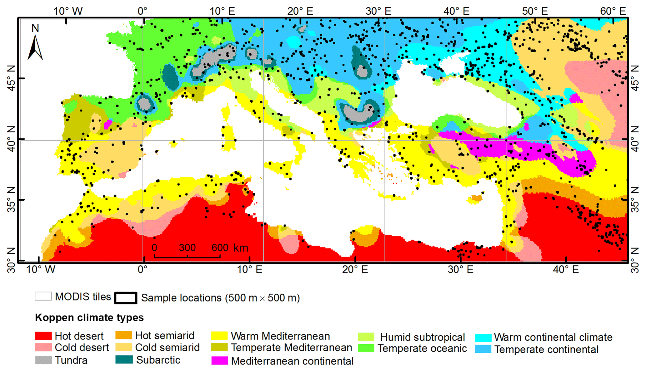
Figure 1Study area and sample locations.
The study region covers 13 climate zones as defined by Peel et al. (2007) (Fig. 1). Numerous water bodies of different types are found in this region, including large coastal lagoons, fresh, brackish or salt marshes, riverine forests and reed beds, flood plains and wet meadows, mountainous lakes and surrounding wetlands, salted lakes, temporary marshes, and streams (Costa et al., 1996). Our study area accounts for 25 % of the world's Ramsar sites that contain a great ecological, social, and economic value, especially as they provide habitat, reproduction, and migration stopover sites for numerous bird species (Galewski, 2012). A good number of the water bodies and wetlands in the region are small, shallow, and highly variable between seasons and years due to weather effects and human activities (Costa et al., 1996).
Many Mediterranean water resources are degraded mainly due to urbanization, agricultural reclamation, increasing water use for irrigation, and hydraulic works such as dams, dikes, river channeling, and drainage and irrigation networks (Batalla et al., 2004). A number of projects and programs have performed monitoring of surface water and wetlands in the Mediterranean region, such as MWO (http://medwet.org/, last access: 10 July 2019) and the GlobWetland initiative (http://webgis.jena-optronik.de/, last access: 10 July 2019), which highlighted the importance of protecting Mediterranean water resources. However, these projects either performed wetland mapping for a few moments in time (e.g., GlobWetland only covered 1975, 1990, and 2005), or were limited to specific water bodies and wetlands instead of the whole landscape. Although surface water dynamics in the Mediterranean can be analyzed at fine spatial resolution with JRC's GSW, it has large spatial and temporal gaps. Figure 2 shows the percentage of pixels with valid observations in JRC's GSW monthly water history dataset for each month between January 2000 and October 2015 calculated over the entire Mediterranean area. The figure illustrates that no valid observation exists for December in the years 2000–2015 in Mediterranean areas according to the GSW monthly water history map. In addition, less than 10 % of the Mediterranean area has observations for January.
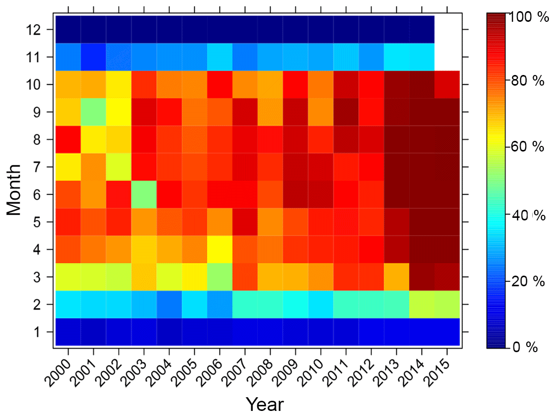
Figure 2Percentage of pixels with valid observations in JRC's Global Surface Water (GSW) monthly water history dataset for each month between January 2000 and October 2015, taken as a spatial average for the entire Mediterranean region as displayed in Fig. 1.
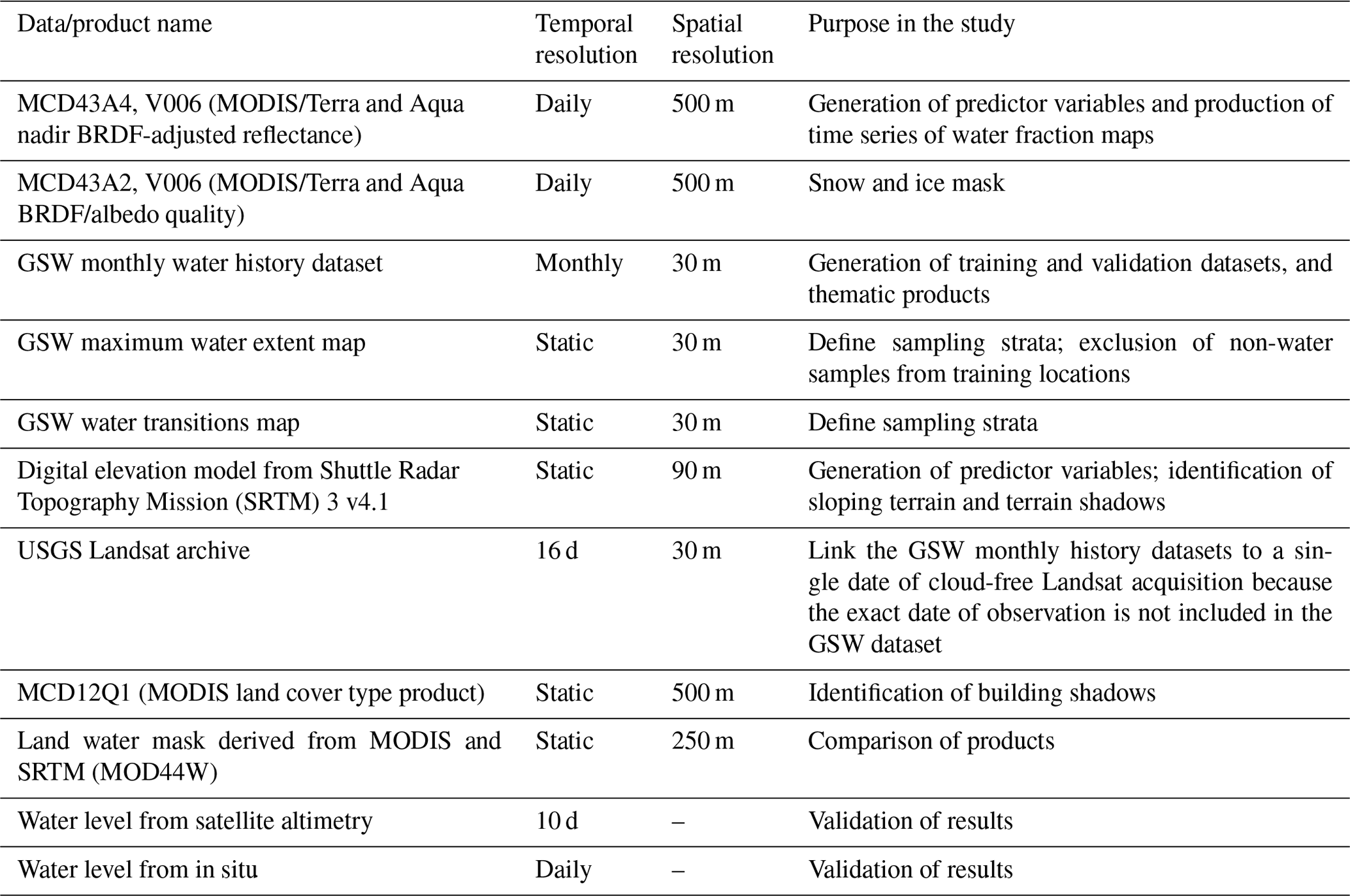
Table 1 summarizes all datasets used in this study. They include a number of sources used to derive model input variables, training data for building the model, validation data for model accuracy assessment, and other existing surface water products against which we compared our products. Details are provided in the following sections.
3.1 MODIS data
The main input dataset in this study is the MODIS Terra and Aqua nadir BRDF-adjusted reflectance (NBAR) product (MCD43A4, V006). This product provides 500 m resolution surface reflectance data for each of the MODIS bands (1–7) corrected to a common nadir view geometry at the local solar noon zenith angle using a bidirectional reflectance distribution function (BRDF) model (Schaaf, 2015b). Compared with the previous collection (V005) that had an 8 d frequency, the V006 collection was retrieved on a daily basis. Each daily value is a result of compositing information obtained during 16 d of observations, which are weighted as a function of the quality, the observation coverage, and the temporal distance from the day of interest. Each daily V006 retrieval is the center (i.e., the ninth day) of the moving 16 d input window (Schaaf, 2015b). We also used the MCD43A2 (V006) Bidirectional Reflectance Distribution Function and Albedo (BRDF/Albedo) Quality dataset to filter out pixels with snow and ice in the MCD43A4 product. This dataset has the same temporal and spatial resolution as MCD43A4 (i.e., daily 500 m resolution), and contains quality information for the corresponding MCD43A4 NBAR product including snow and ice presence (Schaaf, 2015a).
For this study, we downloaded the daily files of MCD43A4 and MCD43A2 for 2000, 2003, 2006, 2009, 2012, and 2015. As explained in Sect. 4.1, all the available dates (or months) of the GSW monthly water history dataset in these 6 years over the sample locations were used for building training and validation data. Instead, when producing the surface water fraction time series, we collected the MCD43A4 and MCD43A2 files using an 8 d time step from February 2000 to December 2017, as processing daily files for the large study area and the 18-year time period would become too time- and memory-consuming. The 8 d repeat coverage is considered to be a minimum for effectively capturing water bodies with short hydroperiods while simultaneously accounting for frequent cloud cover (Guerschmann et al., 2011; Wulder et al., 2016). All images were downloaded from the NASA Earthdata Search website (https://search.earthdata.nasa.gov/search, last access: 10 July 2019).
3.2 Global Surface Water (GSW) dataset
To generate training and validation data for modeling the surface water fraction, we used the GSW dataset (Pekel et al., 2016). This dataset provides the global distribution of the surface water extent at a monthly time interval from March 1984 to October 2015 (380 months) at a 30 m spatial resolution, and also includes a series of thematic maps summarizing different facets of the spatial and temporal dynamics of surface water over 32 years. This dataset is derived from the entire archive of Landsat 5 Thematic Mapper (TM), the Landsat 7 Enhanced Thematic Mapper-plus (ETM+), and the Landsat 8 Operational Land Imager (OLI). Water detection was performed using a dedicated expert system, which was a procedural sequential decision tree that used both the multispectral and multitemporal attributes of the Landsat archive as well as ancillary data layers (Pekel et al., 2016). Based on a validation with very high resolution satellite and aerial imagery, the authors reported a high mapping accuracy with a commission accuracy of 99.45 % and an omission accuracy of 97.01 % (Pekel et al., 2016).
The GSW monthly water history dataset is available in Google Earth Engine (GEE: Gorelick et al., 2017) as an image collection containing 380 images, one for each month between March 1984 and October 2015. Each image provides a binary classification of water presence, or indicates if no valid (cloud-free) Landsat observations were available for a specific pixel and month. For comparison with MODIS data, we used the monthly water history datasets between February 2000 and October 2015, which resulted in 189 images.
Several GSW thematic maps were derived from the GSW monthly water history dataset (Pekel et al., 2016). In this study, we used two thematic maps, the maximum water extent map and the water transitions map, for the Mediterranean region from the data access website (https://global-surface-water.appspot.com/download, last access: 10 July 2019). The maximum water extent map indicates whether each 30 m grid cell was ever detected as water over the 32-year period. The transition map contains 10 water classes: permanent, new permanent, lost permanent, seasonal, new seasonal, lost seasonal, seasonal to permanent, permanent to seasonal, ephemeral permanent, and ephemeral seasonal. It provides information on both intra- and inter-annual variability of surface water (Pekel et al., 2016).
3.3 Terrain data
Terrain data are useful for predicting the locations for water bodies (Drake et al., 2015; Grabs et al., 2009). In this study, we used the near-global Shuttle Radar Topography Mission (SRTM) digital elevation model (DEM) distributed by the Consortium for Spatial Information of the Consultative Group of International Agricultural Research (CGIAR-CSI). This product has a ∼ 90 m resolution and is a post-processed derivative to address areas of missing data in the original SRTM DEM made by the National Aeronautics and Space Administration (Jarvis et al., 2008). The most recent version of this product is SRTM3 v4.1 and is freely available from http://srtm.csi.cgiar.org/ (last access: 10 July 2019).
3.4 Satellite altimetry and in situ water level
We obtained water levels from the U.S. Department of Agriculture Global Reservoir and Lake Monitoring (GRLM) website (http://www.pecad.fas.usda.gov/cropexplorer/global_reservoir, last access: 10 July 2019). This site provides time series of water level variations for some of the world's largest lakes and reservoirs, mainly greater than 100 km2. The GRLM utilizes near-real time data from the Jason-3 mission, and archive data from the Jason-2/OSTM, Jason-1, Topex/Poseidon, and ENVISAT satellites. We also obtained daily in situ gauge observations for Fuente de Piedra Natural Reserve in southern Spain, which were also used in Li et al. (2015).
3.5 Additional data
We utilized the MODIS land cover type product (i.e., MCD12Q1: Friedl et al., 2010) to identify and mask areas that potentially have commission errors related to building shadows. To assess the spatial accuracy of MODIS derived maps, we also used the land water mask derived from MODIS 250 m and SRTM data (MOD44W: Salomon et al., 2004) for comparison.
4.1 Approach for deriving the surface water fraction
The approach used to derived the surface water fraction builds on our previous work (Li et al., 2018) with considerable improvements regarding input data, training data, and commission error processing. We explored the use of MODIS spectral information and a topographic metric for estimating the surface water fraction over two study areas in Spain via the use of rule-based regression models and concluded that a single global regression model can be effectively tuned locally as long as it is fed with training data that comprise the various environmental conditions encountered across the larger area (Li et al., 2018). In this sense, the approach for constructing a global model can be expanded effectively to wider areas such as the Mediterranean region. The following subsections and Fig. 3 describe the individual steps of the approach in detail.
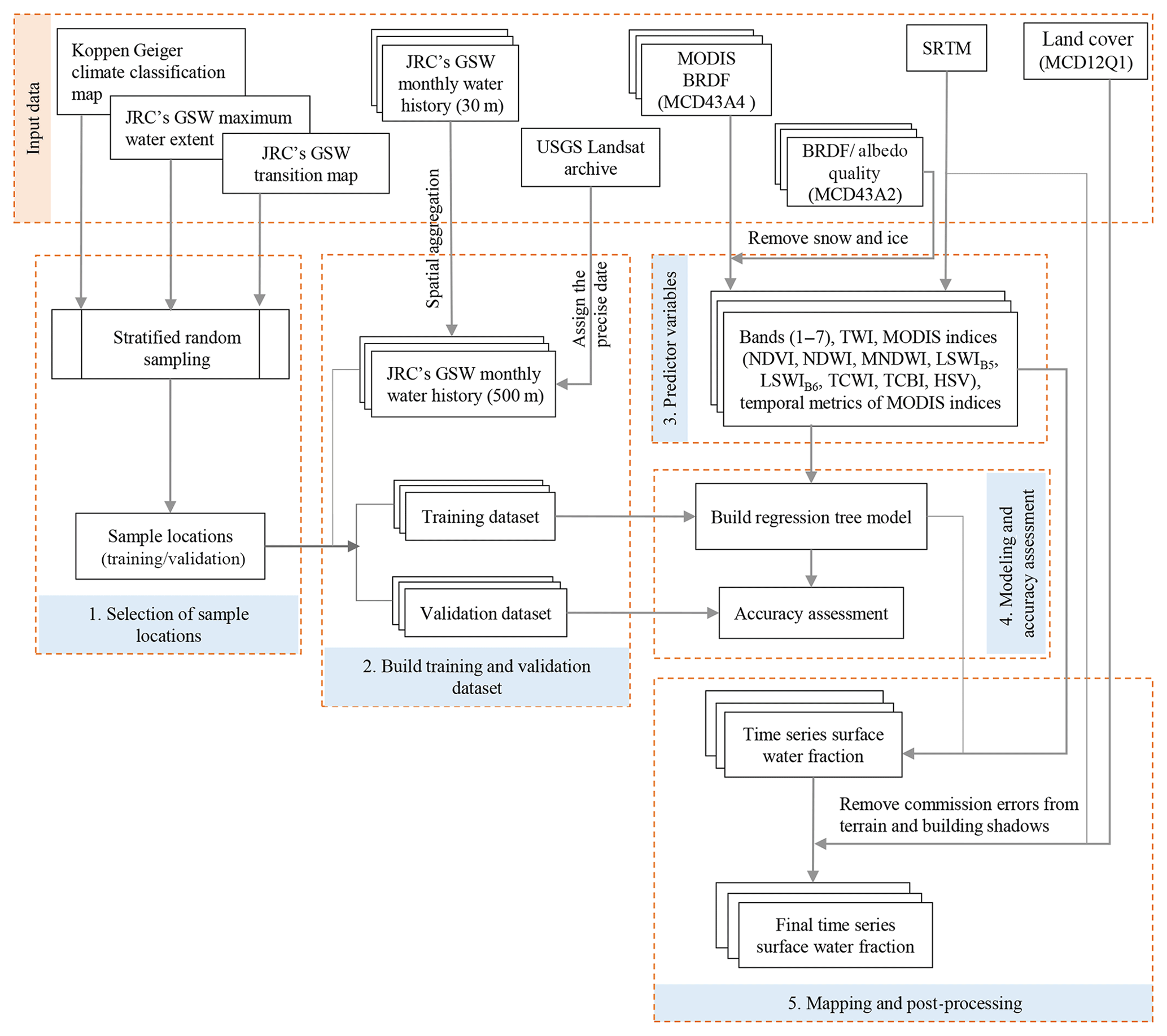
4.1.1 Selection of sample locations for training and validation
Sample locations were selected using a two-stage stratified random sampling method. First, a total of 13 strata were defined based on climate zones (see Fig. 1). We created sampling blocks by partitioning the study area into ∼ 5 km × 5 km grids (i.e., 10×10 MODIS pixels as one block) and assigned each block to the climate zone within its spatial footprint. Blocks that covered more than one climate zone and those that contained no surface water based on the JRC maximum water extent product were excluded from our sample. We then selected 1400 blocks (∼ 2 % of all resulting blocks) using stratified random sampling.
Second, we created 500 m ×500 m grids corresponding to the MODIS geometry in each of the 1400 blocks. A total of 14 strata were defined based on the combination of water fraction categories and water permanence types. Specifically, we first divided all grid cells into seven water fraction categories (0 %, 0 %–20 %, 20 %–40 %, 40 %–60 %, 60 %–80 %, 80 %–100 %, and 100 %) according to the aggregated GSW maximum water extent. Then for each category, we further classified water permanence types based on the aggregated GSW water transitions map. For the 20 %–40 %, 40 %–60 %, 60 %–80 %, 80 %–100 %, or 100 % categories, grid cells were further classified as fluctuating water if they contained more than 20 % fluctuation water otherwise they were assigned as permanent water. For the 0 %–20 % category, grids with 0 % permanent water were classified as fluctuating water, whereas grids with 0 % fluctuation water were classified as permanent water. The rest of the grids in the 0 %–20 % category were not assigned due to a very low water fraction. In the end, the 14 strata were as follows: 100 % permanent, 100 % fluctuating, 80 %–100 % permanent, 80 %–100 % fluctuating, 60 %–80 % permanent, 60 %–80 % fluctuating, 40 %–60 % permanent, 40 %–60 % fluctuating, 20 %–40 % permanent, 20 %–40 % fluctuating, 0 %–20 % permanent, 0 %–20 % fluctuating, 0 %–20 % no water class, and 0 % no water class. From each of the 14 strata, we randomly selected 500 grid cells. This resulted in a set of 7000 MODIS-scale reference grid cells (shown in Fig. 1), which were further split into 3500 training and 3500 validation locations using random sampling from each strata.
Sampling times were selected at a constant interval of 3 years (i.e., 2000, 2003, 2006, 2009, 2012, and 2015). All available dates/months in the GSW monthly history datasets from those selected years were used.
4.1.2 Building training and validation datasets
The GSW monthly water history maps were used for generating training and validation data. Specifically, the 30 m monthly water history maps from all sampling years/months were aggregated to the 500 m resolution for all sample locations in GEE by dividing the 30 m water pixels by the total number of 30 m pixels within each 500 m resolution cell, resulting in a surface water fraction that we used as a reference. Given that the exact dates of these monthly water history maps are not provided with the GSW product, we linked these reference estimates to the USGS Landsat archive that GSW used as its input. For each combination of location/month, we retained only those reference estimates for which the location was covered by a single Landsat tile acquired during that month. If multiple Landsat tiles existed in that month for that location, we only retained the reference estimates if all but one Landsat tile had 100 % cloud cover. In this way, we could accurately assign a precise date to the retained reference estimates.
Surface water fraction estimates derived from all months of the sample years for training locations were used as the training dataset, and the estimates from all sample months for validation locations were used as the validation dataset.
4.1.3 Modeling surface water fraction and accuracy assessment
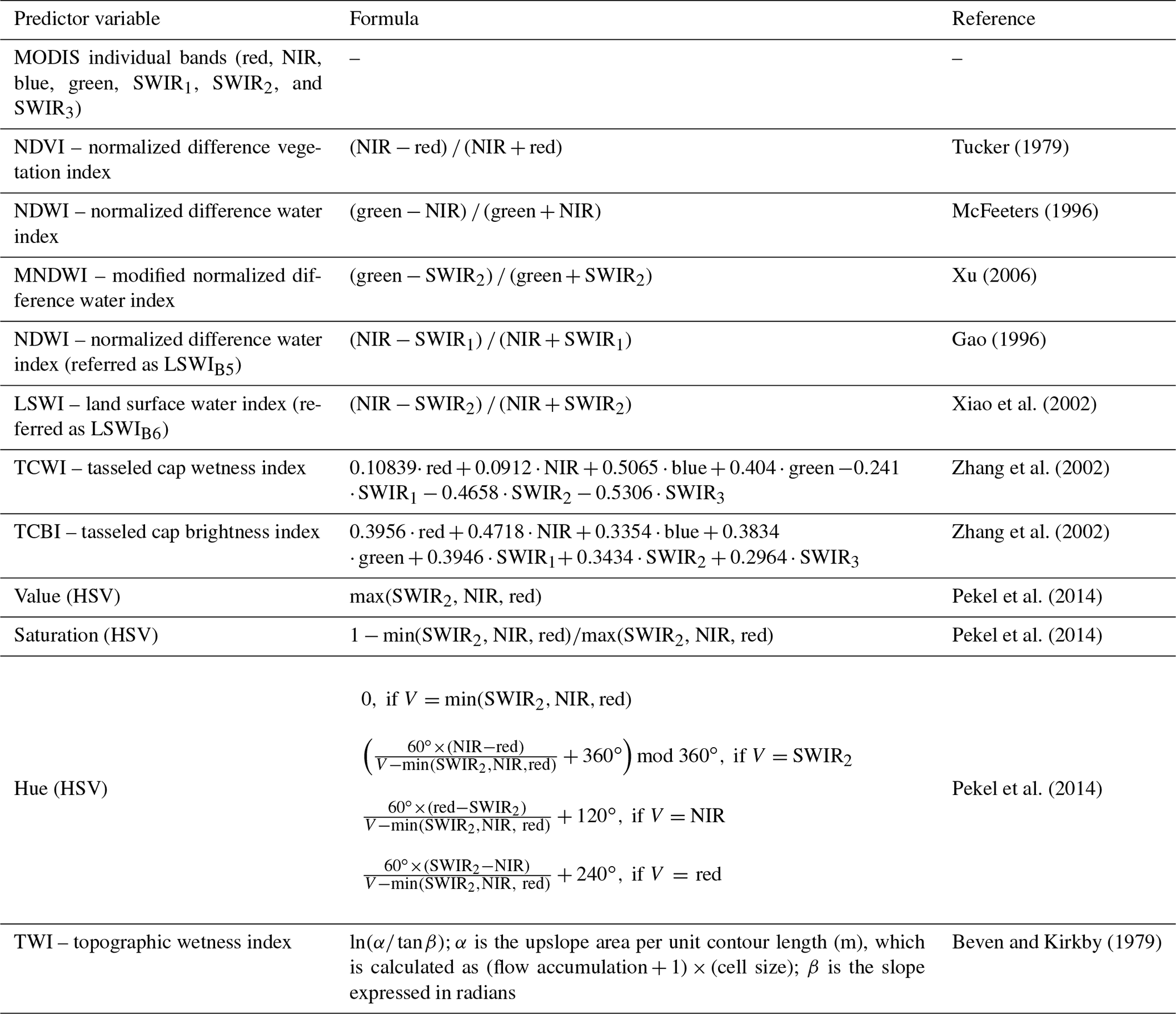
The surface water fraction was estimated using MODIS spectral information and derived water indices, and a topographic metric via a rule-based regression model. All predictor variables (Table 2) evaluated by Li et al. (2018) were used as input for the estimation of surface water fraction. In addition, the annual mean, minimum, maximum, standard deviation, and the coefficient of variation (CV) of each MODIS-derived predictor variable were also included as input in the model. These temporal summaries were demonstrated to be an important input for predicting surface water fraction in our previous study (Li et al., 2018).
Table 2Overview of the predictor variables used in this study. MODIS shortwave infrared bands are referred to as SWIR1 (1230–1250 nm), SWIR2 (1628–1652 nm), and SWIR3 (2105–2155 nm).
Cubist regression models (Quinlan, 1993) contain a set of conditional rules that partition the data space into smaller regions, each of which is linked to a multivariate linear regression model that can predict the explanatory variable (here surface water fraction). Following the findings of our earlier work (Li et al., 2018), we used a single global Cubist regression model, but trained it with data collected from across the study area to tune the model to local conditions. In the global Cubist regression model, two parameters can be defined to optimize accuracy and reduce the instability of the model prediction. The first is called “committees” indicating that multiple model trees are developed in sequence. Each member of the committee predicts the target value and the members' predictions are averaged to give a final prediction (Quinlan, 1993). The second parameter is “neighbors” and allows the Cubist model to group similar samples in terms of predictor variable values, and determine the average prediction of these training samples (Kuhn et al., 2012; Quinlan, 1993). We tuned the models over different values of “committees” and “neighbors” (“committees” was set to be 0, 10 , 20, 50, and 100, and “neighbors” was set to be 0, 1, 5, and 9) through a 10-fold cross-validation on our training data and selected the values that produced the smallest root mean square error (RMSE).
The resulting model was evaluated on both the training data that were used to generate the model and the independent validation data (Sect. 4.1.2). Three statistical measures were used to assess model performance: the coefficient of determination (R2), mean absolute error (MAE), and the RMSE.
4.1.4 Mapping and post-processing
We applied the resulting model to the MCD43A4 V006 data from February 2000 to December 2017 to produce gridded time series of surface water fraction for the Mediterranean region with an 8 d time step resulting in 46 maps per year (except for 2000, which only contained 39 images).
Recent studies on surface water detection using optical sensors showed that multiple sources of commission errors exist, such as terrain and building shadows (Klein et al., 2017; Pekel et al., 2016). These errors can be accounted for using masks derived from auxiliary data (Klein et al., 2017; Pekel et al., 2016). In this study we addressed two sources of commission errors: shadows from buildings and identified surface water presence that is unlikely on sloping terrain. Specifically, a slope map was derived from the SRTM DEM by calculating the maximum rate of change in elevation from each raster cell to their eight neighbors. We then used a threshold of 5∘ to identify steep locations where it is unlikely to find surface water but could have been detected as water by our model, for example, due to spectral confusion between water and terrain shadows (Yamazaki et al., 2015). In the case of building shadows, we used the urban class of the MODIS classification product MCD12Q1 (Friedl et al., 2010) to assign areas potentially affected by building-induced shadows. Pixels were reassigned to the 0 % water fraction for slopes steeper than 5∘ and for areas classified as urban in MCD12Q1, except for places where water was present according to the GSW maximum water extent.
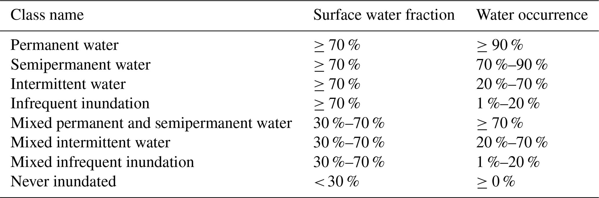
Table 3Seasonality classification criteria based on surface water fraction and occurrence. The occurrence indicates how often the specified surface water fraction is reached for a single hydrological year (October 2014–September 2015).
4.2 Generation of the surface water fraction metrics and comparison of products
Based on gridded time series of surface water fraction, we derived a series of ecologically relevant metrics that capture both the intra- and inter-annual variability and changes, and further compared these metrics with GSW-derived thematic products. The readily available GSW thematic products were derived from 32 years of data (between March 1984 and October 2015); thus, they cannot be directly compared against our MODIS-based results for 2000–2017. Therefore, we reproduced the GSW thematic maps using the GSW monthly water history dataset from the overlapping period of these two datasets (i.e., February 2000–October 2015). We then also computed the MODIS-derived temporal metrics for this period. In total, 189 GSW water history images and 720 surface water fraction maps were incorporated for the generation of these thematic maps. The following metrics were generated:
-
The annual maximum and mean annual maximum surface water fraction between 2000 and 2015: the GSW monthly water history maps were summarized for each year in GEE to calculate the annual maximum surface water extent. We then aggregated the results of each year to the MODIS resolution and averaged all years to derive the mean annual maximum surface water fraction. To assess the spatial agreement of the mean annual maximum surface water fraction derived from MODIS and GSW, we calculated the surface water area (in km2) from the mean annual maximum surface water fraction using a threshold continuum. Specifically, the surface water fraction was partitioned using nine threshold values set in 10 % increments from 0 % to 100 %. All pixels with a surface water fraction greater than or equal to the threshold were summed and then multiplied by the MODIS pixel size. We then compared the water area (in km2) derived from the mean annual maximum surface water fraction based on GSW and MODIS across a different continuum of threshold values. We also compared the water area with the 250 m static water mask from MOD44W.
-
The standard deviation of the annual maximum: a measure of the inter-annual variability of water presence.
-
The seasonality: a measure for the seasonal and intra-annual variability of water presence. We calculated the number of times (i.e., the water occurrence) a given pixel displayed standing water above a certain water fractional threshold for a single hydrological year (October 2014 to September 2015), as GSW has a relatively large number of valid observations for this year (Fig. 2), and then classified different types of water permanence. The water occurrence was calculated for each grid cell as a fraction of the number of times water was present relative to the total valid observations (i.e., not affected by clouds). We adopted the classification criteria of Guerschmann et al. (2011) and further modified it to be applicable to the Mediterranean region (Table 3). As the classes are not mutually exclusive, they are prioritized in the order shown in Table 3.
4.3 Demonstrating the representation of surface water dynamics by the new MODIS dataset
To assess the performance of our MODIS-derived product for monitoring temporal variations in the surface water extent, we selected three lakes with fluctuating water presence. These three sites have varying sizes, and different geographic locations and temporal dynamics, and have also been listed in the International Conventions on Wetlands (known as Ramsar) given their importance for staging and wintering waterfowl. The three sites are as follows:
-
The Fuente de Piedra lake, Spain, which is a shallow and saline lake, has a maximum area of 13.6 km2. It experiences strong seasonal, inter-annual, and intra-annual variations of water level and inundation extent (Li et al., 2015).
-
Lake Sabkhat al-Jabbul, Syria, which is a large, permanent saline lake that is surrounded by semiarid steppe. At high water levels, it contains two islands; it traditionally floods in the spring and shrinks back during the summer and autumn but seldom dries out completely (JAES-CC, 2010).
-
The coastal marshland complex of Doñana, Spain, which is separated from the ocean by an extensive dune system and is subject to seasonal and inter-annual variations in water level (De Castro and Reinoso, 1997).
For the first two lakes, we compared the time series of the MODIS-derived surface water area with that from GSW, and further compared these against water level data from satellite altimetry or in situ measurements. We calculated the Spearman rank correlation (ρ) between water level and water area derived from MODIS SWF and JRC's GSW data to assess the correspondence between these datasets. For Doñana, we compared the monthly spatial distribution of the surface water extent derived from MODIS and JRC's GSW. To ensure the accuracy of the area calculations, we only calculated an area for times when it contained at least 95 % of valid data from MODIS SWF and JRC's GSW data.
5.1 Model performance
Following the model tuning of the Cubist regression model (see Sect. 4.1.3), we found that a 20-member committee and 9-neighbor model resulted in the smallest RMSE between the actual (GSW-derived) water fraction and our MODIS-based water fraction estimates. The addition of more committees or neighbors had little effect on the accuracy.
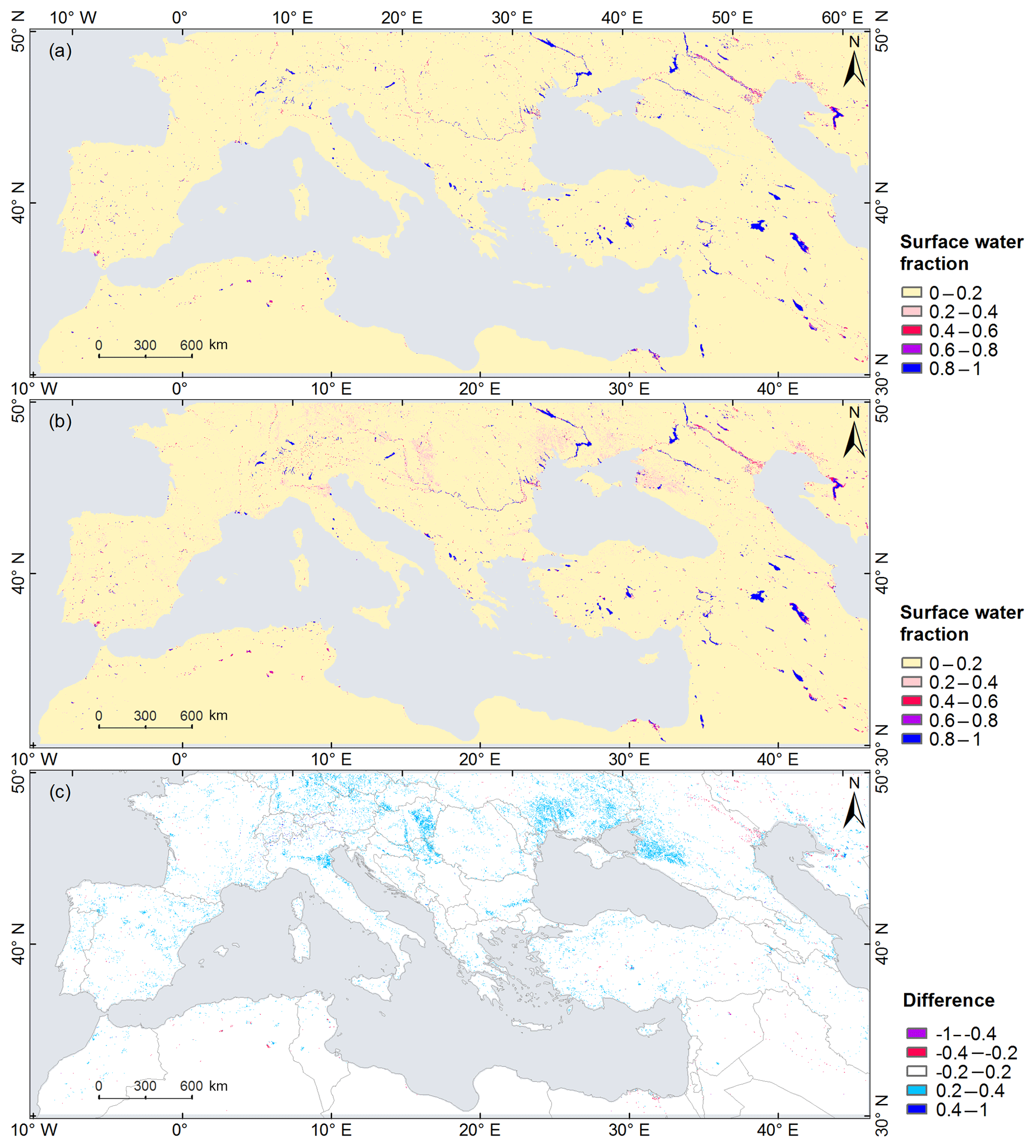
Figure 4Mean annual maximum surface water fraction maps as obtained from (a) JRC's GSW and (b) MODIS time series surface water fraction for the period from 2000 to 2015, and (c) the difference between the two maps. Positive difference values indicate that our MODIS dataset detected a larger water fraction than JRC's GSW.
Table 4Statistical measures between the predicted surface water fraction and the actual data for training and validation data, and for different types of water permanence using validation data.
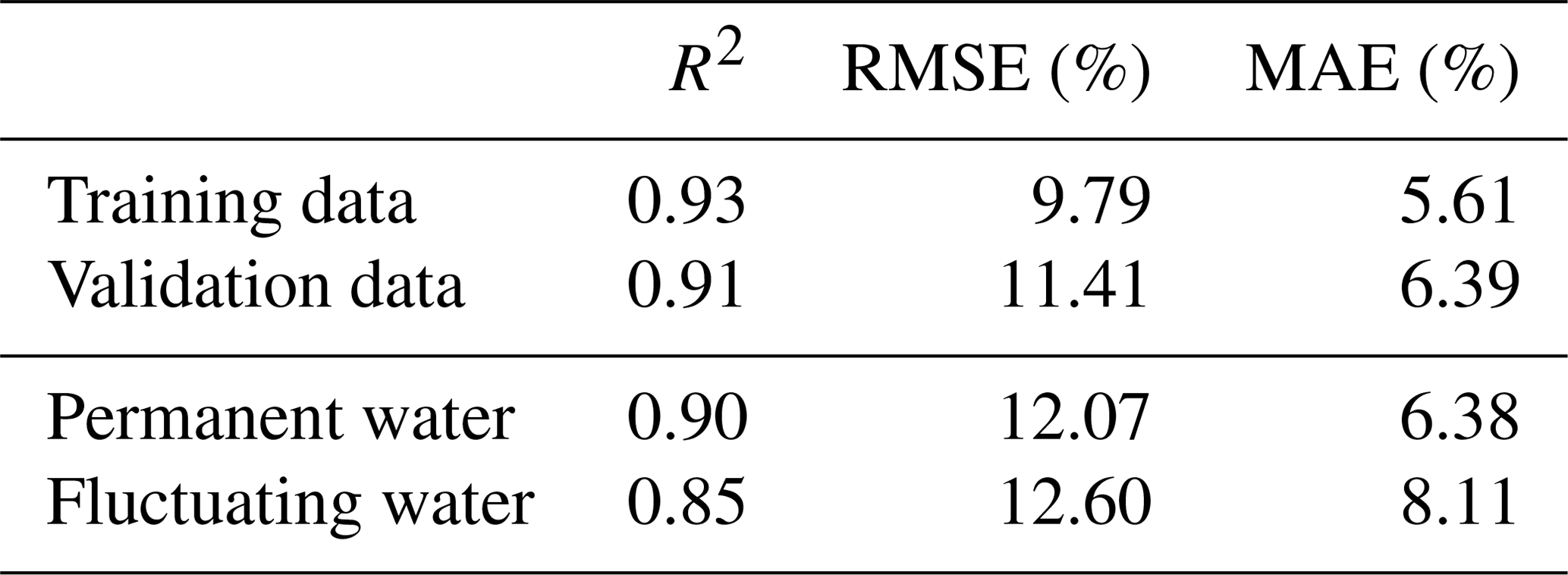
Table 4 shows the statistical measures between the predicted and actual surface water fraction. The model predicted surface water fraction shows good agreement with the actual value with an R2 of 0.93 for the training data. When testing using the independent validation dataset, the R2 value is only slightly smaller, and the RMSE and MAE are slightly larger, suggesting that the Cubist regression model does not suffer from overfitting. The RMSE and MAE for fluctuating water were slightly larger than for permanent water (Table 4). This suggests that the developed model not only provides accurate results for the static mapping of the surface water fraction, but it can also be applied effectively for monitoring the dynamics of fluctuating surface water.
5.2 Surface water fraction metrics and comparison of products
The mean annual maximum surface water fraction values generated from GSW and the MODIS-derived product over the 2000–2015 period are displayed in Fig. 4. Overall, the two maps are in good agreement. Visual comparison indicates that our MODIS-derived product is able to detect narrow rivers with widths covering a couple of MODIS pixels, such as the Danube, Euphrates, Po, Rhine, and Tagus rivers. Large differences are evident for some low surface water fraction regions such as parts of Hungary and the Ukraine (Fig. 4). These differences likely correspond to the presence of wet meadows, salt marshes, and floodplains along large rivers, which are usually saturated and inundated with water during most of the vegetative season (Šefferová Stanová et al., 2008; Stefan et al., 2016). Around the Po River in Italy, where rice paddies are seasonally present, our MODIS product also shows larger surface water fractions (Fig. 4c). This result suggests that the MODIS-derived surface water fraction has enhanced sensitivity to surface water in wetland areas with emerged vegetation, and this could be attributed to the fact that several predictor variables such as LSWI (Xiao et al., 2002) are also sensitive to vegetation water content (Li et al., 2015). Table 5 confirms that the total surface water areas for the Mediterranean calculated from MODIS are more comparable to the GSW results when only considering areas with a higher surface water fraction. For example, when only accounting for pixels with surface water fractions equal to or greater than 50 %, the total surface water areas for the Mediterranean based on both datasets are similar (75 107 km2 for GSW versus 73 444 km2 for MODIS). In comparison, only 70 543 km2 of water was detected in this region based on the 250 m static water mask from MOD44W. This implies that our MODIS product detects more surface water than other coarse-resolution binary maps. Nonetheless, our MODIS product detects less surface water than GSW for larger thresholds (≥50 %), whereas it detects much more surface water than GSW for small thresholds (≤20 %). This confirms an earlier finding that machine learning approaches such as Cubist and random forest often underestimate large values and overestimate small values when estimating the fractional cover of land surface (e.g., Huang et al., 2014; Li et al., 2018; Wang et al., 2017). In addition to the effects of mixed pixels (Klein et al., 2017), the most obvious reason for this is because regression techniques used in such approaches fit linear equations to relationships that may not be linear over the entire range of values.
Table 5Comparison of total surface water area (in km2) as determined from JRC's GSW and MODIS mean annual maximum surface water fraction maps for different thresholds.
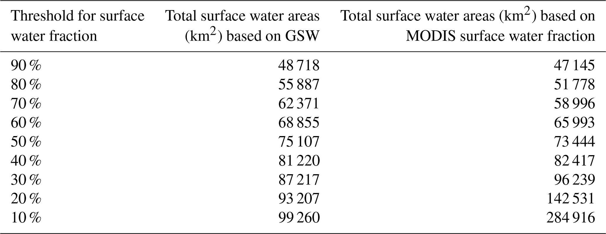

Figure 5Standard deviation of the surface water fraction as calculated from (a) JRC's GSW and (b) MODIS annual maximum surface water fraction maps for the period from 2000 to 2015.
Figure 5 shows the standard deviation of the annual maximum surface water fraction. It indicates that areas of large inter-annual variability agree between MODIS-based and GSW-based results. Both indicate a larger variability in the surface water fraction in semiarid and desert climate zones, particularly in the north of Algeria, for the Volga Delta in the Caspian depression, and along the Tigris and Euphrates rivers of Iraq.
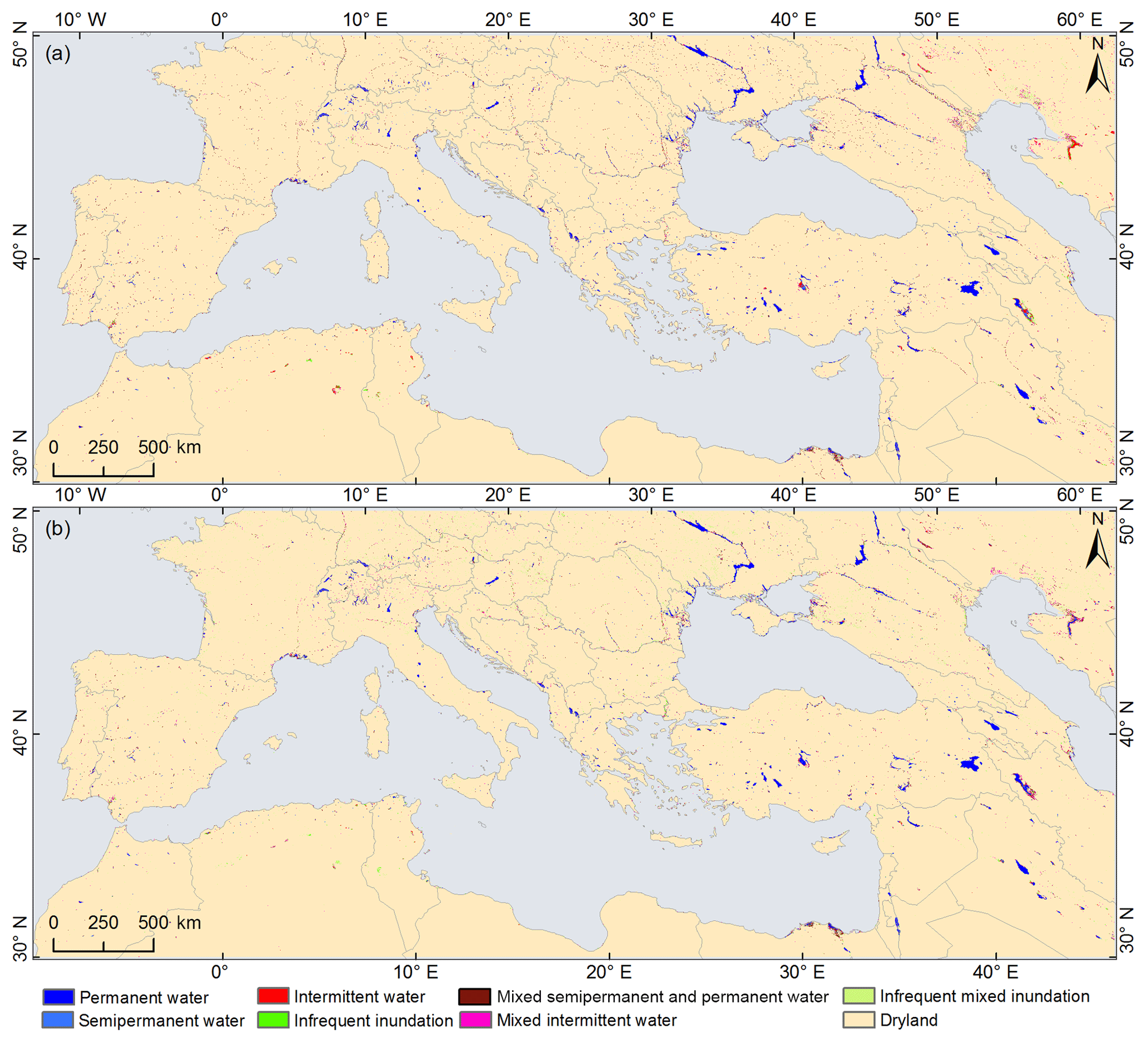
Figure 6Seasonality information derived from time series of the (a) JRC's GSW and (b) MODIS surface water fraction for a single year (October 2014 to September 2015).
Figure 6 displays the seasonality metric for the entire study area, with details for two selected sites shown in panels (a) and (b) of Figs. 7 and 8. Fuente de Piedra is a seasonally flooded lake which usually dries out completely in summer (May–September) (Batanero et al., 2017; Li et al., 2015) with the exception of extremely wet years (e.g., 2010, 2011, 2013: Rodriguez-Rodriguez et al., 2016) when water was present throughout the whole year. The differences in water seasonality for Fuente de Piedra between the two products (Fig. 7a, b) can be attributed to the fact that GSW lacks observations in wet seasons, resulting in a reduced water occurrence compared with our MODIS product. The discontinuities in the Landsat record between seasons can affect the accuracy of seasonality information, which has also been demonstrated by Klein et al. (2017) and Pekel et al. (2016). Permanent water is present in parts of Lake Sabkhat al-Jabbul, but the larger central portion of the lake has highly dynamic intermittent water (Fig. 8). Mixed permanent and semipermanent waters are mostly found on the edge of permanent water and in narrow rivers.
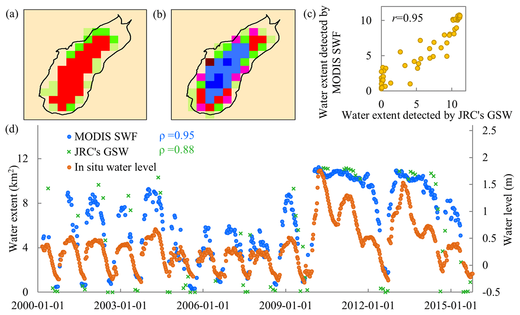
Figure 7Seasonality information derived from (a) JRC's GSW and (b) the MODIS surface water fraction from a single year (October 2014 to September 2015). The colors in (a) and (b) are the same as in Fig. 6. (c) A scatterplot of the water area obtained from JRC's GSW versus that from MODIS SWF. r represents the Pearson correlation between two datasets. (d) A comparison of time series of the surface water area (in km2) derived from JRC's GSW (shown using green asterisks) with MODIS surface water fraction (shown using blue dots) from 2000 to 2015, along with in situ water level data (shown using orange dots) for Fuente de Piedra, Spain. ρ represents the Spearman rank correlation between the water level and water area.
5.3 MODIS-derived surface water dynamics for selected lakes
Panels (d) of Figs. 7–8 show the time series of the surface water extent detected by MODIS and GSW for two selected lakes. Fuente de Piedra (Fig. 7d) experiences large temporal variability in the surface water extent throughout the year, which is well represented by our MODIS product with 461 time steps (Table 6). This variability corresponds closely to the in situ water level data (ρ=0.95). Note that in extreme wet years (i.e., 2010, 2011, and 2013), the lake remained flooded throughout the year without increasing in size with regard to water level changes (Rodriguez-Rodriguez et al., 2016). The water extent derived from MODIS SWF also matched closely to that from GSW (Fig. 7c, d; r=0.95). GSW only had 73 valid time steps with most observations in dry seasons (i.e., June to October); thus, it did not allow for the appropriate capture of the seasonal dynamics, particularly for the November–March period when the lake usually reaches its full surface water extent. Time series of the water extent of Lake Sabkhat al-Jabbul as determined by our MODIS product showed a relative high correlation with water level data (ρ=0.69). It also showed good agreement with the water extent derived from GSW, including the seasonal peak extent and the minimum surface water extent during the dry season (Fig. 8c, d; r=0.88). This implies that the coarse 500 m MODIS data not only provide more detailed temporal information (563 MODIS surface water fraction time steps versus 69 GSW time steps) (Table 6), but they also give accurate estimations of the surface water area compared with the results from Landsat 30 m resolution data.
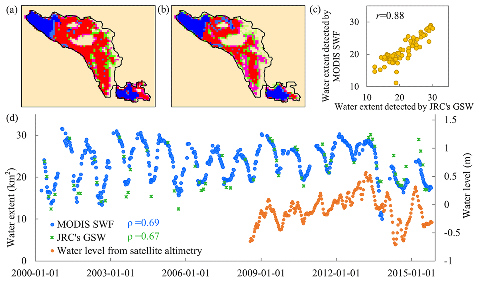
Figure 8As in Fig. 7, but for Lake Sabkhat al-Jabbul, Syria. The water level for this lake is computed from Jason-2/OSTM altimetry and repeats every 10 d.
Table 6Number of valid temporal observations for the three lakes based on the MODIS surface water fraction and JRC's GSW between February 2000 and October 2015.
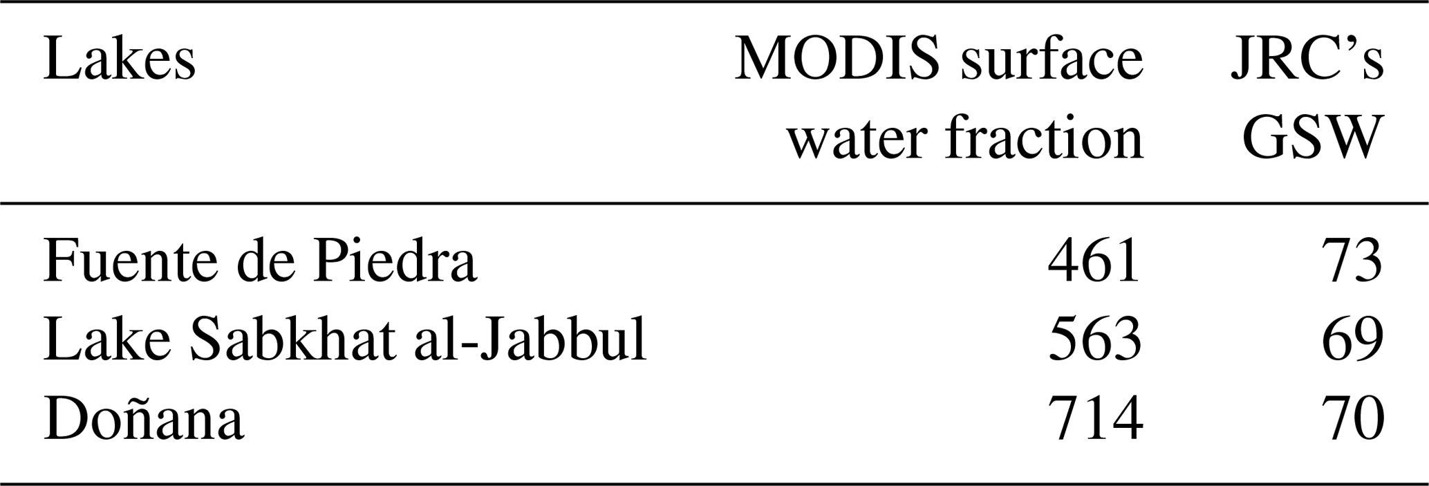
Figure 9 compares the MODIS monthly surface water fraction with the GSW monthly water history for Doñana, Spain. The visual comparison shows that the distribution of the MODIS surface water fraction agrees well with the GSW monthly water maps. The 500 m MODIS surface water fraction is able to capture the spatial patterns as detected from the high-resolution Landsat-based GSW dataset. Seasonal drying out and flooding of the wetland is well detected with the MODIS-derived surface water fraction, whereas GSW lacks temporal details, for example, during large water extents in November and December. MODIS also captures the timing of the maximum water extent (i.e., in January) and water retreat (i.e., in July). This example highlights that the information provided by our MODIS product can contribute to a better understanding of surface water dynamics.
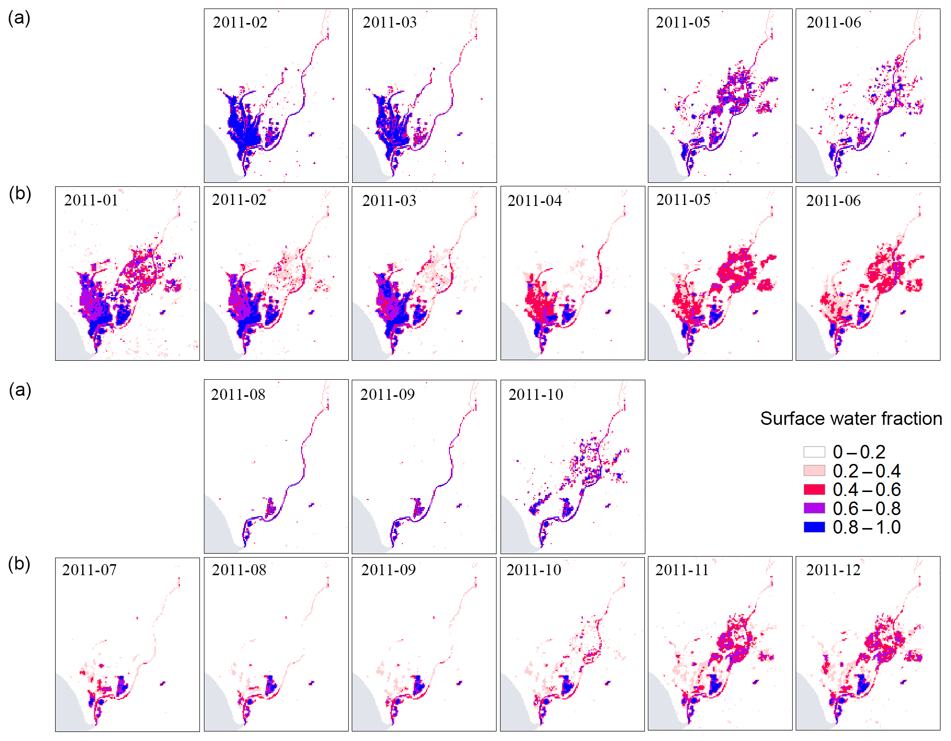
Figure 9Comparison of monthly water distribution based on (a) the Landsat-based GSW dataset and (b) the MODIS surface water fraction for Doñana, Spain, for 2011.
We estimated the surface water fraction for the Mediterranean region from MODIS data, and improved on previous efforts to estimate surface water fraction from medium-resolution imagery (MODIS or similar). The prediction accuracy of our model (R2=0.91, RMSE =11.41 %, and MAE =6.39 %) is higher than the R2 of 0.625 reported by Weiss and Crabtree (2011), who used a linear regression model, and the R2 of 0.7 reported by Guerschmann et al. (2011), using a logistic regression model. This research successfully expanded our previous work (Li et al., 2018) by upscaling it from a relatively small region to the whole Mediterranean while retaining a similar high accuracy (both achieved an R2 of 0.91). This attributes to the feasibility and robustness of Cubist regression modeling with respect to dealing with different environmental conditions when training data are collected across a wide geography resulting in varying spectral characteristics.
Secondly, we generated surface water fraction maps at high temporal frequency, which is an advantage over existing fine-resolution datasets. Our MODIS-derived surface water fraction product accurately displays the spatiotemporal variability of surface water. The comparison with the GSW 30 m product and water level data (Figs. 7–9) reveal that our product can efficiently monitor the seasonal, intra-annual, and long-term surface water dynamics with good spatial and temporal accuracy. For example, it complements the GSW by allowing for the detection of inundation and recession processes over short time periods and for the better representation of seasonality changes and temporal trends over longer periods. The MODIS surface water fraction can also accurately detect the spatial distribution of surface water inclusive of small water bodies (less than one MODIS pixel) and narrow rivers, which are missing in other coarse-resolution products using binary classification method such as MOD44W (Salomon et al., 2004). Metrics derived from the MODIS surface water fraction and GSW time series can reflect different facets of surface water dynamics. The accuracy of some metrics, such as seasonality, relies on the number of valid observations and the temporal interval. Landsat-derived metrics might be problematic in areas with large temporal gaps caused by persistent cloud cover, as shown in this study (Fig. 8) and previously by Pekel et al. (2016) and Klein et al. (2017). Although cloud coverage also limits MODIS observations, the probability of obtaining cloud-free observations is higher (Table 6) due to the daily acquisitions and consequent temporal compositing possibilities. With these advantages, we expect that our MODIS surface water fraction product could fill in important information on surface water for areas and time periods for which cloud-free Landsat acquisitions are few or non-existent.
Our MODIS-derived surface water fraction product also has limitations. Firstly, it is designed to detect only open surface water; therefore, it may not effectively capture water bodies covered by dense vegetation, such as swamps, lakes with considerable coverage of aquatic vegetation, and inundated dense forests. Secondly, the MODIS surface water fraction product overestimates small surface water fractions of less than 20 % (Table 5), which has also been found in previous studies on surface water fraction mapping (Li et al., 2018; Parrens et al., 2017). This overestimation might be attributed to the mixed spectral response of pixels with different land cover types, as already demonstrated by many studies (e.g., Guerschmann et al., 2011; Klein et al., 2017). Further work could consider reassigning pixels with less than 20 % surface water to 0 % water fraction for locations where water is never present according to the GSW maximum water extent. Thirdly, the auxiliary layers utilized for the identification of potential areas of commission errors also appear to have some limitations. For example, some urban areas might be not mapped in MCD12Q1, and areas of cloud cover and cloud shadow might not be completely removed from the MCD43A4 product. The importance of these limitations may diminish as the quality of these auxiliary layers improves or dynamic datasets rather than static layers are incorporated (e.g., Global Human Settlement Layer: Pesaresi et al., 2016). Fourthly, the MCD43A4 product also suffers from many missing values, especially in regions with large amounts of precipitation, aerosol concentrations, or snow and ice coverage (Klein et al., 2017). Future research should focus on combining other moderate-resolution data (e.g., MOD09) for areas with missing data to ensure a gap-free reconstruction of inland water development for the past and future.
This work can be further scaled up over much larger regions and for shorter (e.g., daily) time intervals. A high-quality training dataset is crucial for the effective application of the rule-base regression model and the collection of such training data is time consuming (Sun et al., 2012). In this paper, time series of the GSW monthly water history dataset proved to be an efficient basis for building a reliable training dataset. Considering that GSW is globally available, we are confident that our approach can be scaled to monitor the surface water fraction globally with MODIS data. Although the surface water fraction maps were produced with an 8 d time step, the model developed in this paper was actually trained using daily MODIS data and could be directly applied to that temporal resolution. The resulting daily surface water fraction maps could be of high interest for ecological and hydrological research. The recent GCOS report requires water extent and lake ice cover with a daily temporal resolution and a 20 m and 300 m spatial resolution, respectively (Belward, 2016). Our approach makes this requirement for the coarser of the two resolutions within reach.
Our MODIS surface water fraction dataset may benefit a large number of applications. For example, it could be used as a monitoring tool for analyzing hydrologic extremes such as floods and droughts, detecting abnormal changes of wetland hydrology, capturing short-duration events, identifying newly formed and disappearing water bodies, and estimating global water loss. The MODIS surface water fraction dataset may help to improve the calibration and validation of hydrological models. For example, the water area can help to estimate a series of hydrological parameters such as water discharge (Huang et al., 2018) and water volume (Busker et al., 2019; Cael et al., 2017; Duan and Bastiaanssen, 2013; Tong et al., 2016). This would be particularly useful for areas where in situ measurements are sparse or inaccessible. Closely monitoring hydrological variability is important for understanding how climate change, meteorological variability, and human activities affect the dynamics of surface water and human livelihoods (Tulbure and Broich, 2019; Zhang et al., 2019). It may also provide new insights for understanding how surface water dynamics further influence climate. For example, lake expansion and the creation of new dams can alter local and regional precipitation patterns (Ekhtiari et al., 2017; Hossain et al., 2009; Mohamed Degu et al., 2011). Similarly, our long-term records and derived metrics have the potential to contribute to the management and conservation of biodiversity and other ecosystem services associated with terrestrial surface water and wetlands.
We derived an 8 d, 500 m resolution surface water fraction product over the Mediterranean for the period from 2000 to 2017 by applying a global Cubist regression tree model to MODIS and SRTM data. We validated the results with JRC's Landsat-derived GSW dataset, which resulted in a high overall accuracy (R2=0.91, RMSE =11.41 %, and MAE =6.39 %). The MODIS-derived surface water fraction showed a good spatial and temporal correspondence with JRC's GSW. Comparison with satellite altimetry and in situ water level data for selected lakes demonstrated the ability of MODIS surface water fraction to effectively monitor seasonal and inter-annual changes in surface water extent. Our dataset provides a consistent, long-term record (18 years) of 8 d water fraction dynamics for the Mediterranean region, and complements fine spatial resolution surface water products, especially in regions where such products have long temporal and spatial data gaps due to both the limited number of acquisitions and persistent cloud cover. Our approach is also promising for monitoring surface water fraction at the global scale and at a daily interval.
The final derived 18 years of surface water fraction maps for the Mediterranean region are available from https://doi.org/10.17026/dans-xrz-y92s (Li, 2019). The GEE and R code used for this paper are available upon request from the first author.
LL and VA designed the experiment. LL performed all analysis and developed the 18-year database. LL prepared the paper with contributions from all co-authors. All authors approved the final version of the paper.
The authors declare that they have no conflict of interest.
This article is part of the special issue “Hydrological cycle in the Mediterranean (ACP/AMT/GMD/HESS/NHESS/OS inter-journal SI)”. It is not associated with a conference.
We would like to thank Alan Belward and Jean-François Pekel (Joint Research Centre) for their support in accessing the global surface water datasets. Many thanks to the authorities of the Fuente de Piedra Natural Reserve and the Junta de Andalucía for providing the in situ water level data used in this study. We also thank Willem Nieuwenhuis for his technical support.
This paper was edited by Eric Martin and reviewed by two anonymous referees.
Batalla, R. J., Gómez, C. M., and Kondolf, G. M.: Reservoir-induced hydrological changes in the Ebro River basin (NE Spain), J. Hydrol., 290, 117–136, https://doi.org/10.1016/j.jhydrol.2003.12.002, 2004.
Batanero, G. L., León-Palmero, E., Li, L., Green, A. J., Rendón-Martos, M., Suttle, C. A., and Reche, I.: Flamingos and drought as drivers of nutrients and microbial dynamics in a saline lake, Sci. Rep., 7, 12173, https://doi.org/10.1038/s41598-017-12462-9, 2017.
Belward, A.: The global observing system for climate: Implementation needs, Technical Report, GCOS-200, World Meteorological Organization, 2016.
Beven, K. J. and Kirkby, M. J.: A physically based, variable contributing area model of basin hydrology/Un modèle à base physique de zone d'appel variable de l'hydrologie du bassin versant, Hydrol. Sci. Bull., 24, 43–69, https://doi.org/10.1080/02626667909491834, 1979.
Busker, T., de Roo, A., Gelati, E., Schwatke, C., Adamovic, M., Bisselink, B., Pekel, J.-F., and Cottam, A.: A global lake and reservoir volume analysis using a surface water dataset and satellite altimetry, Hydrol. Earth Syst. Sci., 23, 669–690, https://doi.org/10.5194/hess-23-669-2019, 2019.
Cael, B. B., Heathcote, A. J., and Seekell, D. A.: The volume and mean depth of Earth's lakes, Geophys. Res. Lett., 44, 209–218, https://doi.org/10.1002/2016GL071378, 2017.
Carroll, M. L., Townshend, J. R., DiMiceli, C. M., Noojipady, P., and Sohlberg, R. A.: A new global raster water mask at 250 m resolution, Int. J. Dig. Earth., 2, 291–308, https://doi.org/10.1080/17538940902951401, 2009.
Chahine, M. T.: The hydrological cycle and its influence on climate, Nature, 359, 373–380, https://doi.org/10.1038/359373a0, 1992.
Cole, J. J., Prairie, Y. T., Caraco, N. F., McDowell, W. H., Tranvik, L. J., Striegl, R. G., Duarte, C. M., Kortelainen, P., Downing, J. A., Middelburg, J. J., and Melack, J.: Plumbing the global Carbon cycle: Integrating inland waters into the terrestrial Carbon budget, Ecosystems, 10, 172–185, https://doi.org/10.1007/s10021-006-9013-8, 2007.
Costa, L. T., Farinha, J. C., Hecker, N., and Tomàs-Vives, P.: Mediterranean Wetland Inventory: A reference manual, MedWet/Instituto da Conservação da Natureza/Wetlands International publication, Volume I, Portugal, 1996.
De Castro, F. and Reinoso, J. C. M.: Model of long-term water-table dynamics at Donana National Park, Water Res., 31, 2586–2596, https://doi.org/10.1016/s0043-1354(97)00098-5, 1997.
Donchyts, G., Baart, F., Winsemius, H., Gorelick, N., Kwadijk, J., and van de Giesen, N.: Earth's surface water change over the past 30 years, Nat. Clim. Chang., 6, 810–813, https://doi.org/10.1038/nclimate3111, 2016.
Drake, J. C., Jenness, J. S., Calvert, J., and Griffis-Kyle, K. L.: Testing a model for the prediction of isolated waters in the Sonoran Desert, J. Arid Environ., 118, 1–8, https://doi.org/10.1016/j.jaridenv.2015.02.018, 2015.
Du, Y., Zhang, Y. H., Ling, F., Wang, Q. M., Li, W. B., and Li, X. D.: Water bodies' mapping from Sentinel-2 imagery with Modified Normalized Difference Water Index at 10-m spatial resolution produced by sharpening the SWIR band, Remote Sens., 8, 354, https://doi.org/10.3390/rs8040354, 2016.
Duan, Z. and Bastiaanssen, W. G. M.: Estimating water volume variations in lakes and reservoirs from four operational satellite altimetry databases and satellite imagery data, Remote Sens. Environ., 134, 403–416, https://doi.org/10.1016/j.rse.2013.03.010, 2013.
Ekhtiari, N., Grossman-Clarke, S., Koch, H., Meira de Souza, W., Donner, R. V., and Volkholz, J.: Effects of the lake Sobradinho reservoir (Northeastern Brazil) on the regional climate, Climate, 5, 50, https://doi.org/10.3390/cli5030050, 2017.
Feng, M., Sexton, J. O., Channan, S., and Townshend, J. R.: A global, high-resolution (30-m) inland water body dataset for 2000: first results of a topographic–spectral classification algorithm, Int. J. Digit. Earth, 9, 113–133, https://doi.org/10.1080/17538947.2015.1026420, 2015.
Friedl, M. A., Sulla-Menashe, D., Tan, B., Schneider, A., Ramankutty, N., Sibley, A., and Huang, X.: MODIS Collection 5 global land cover: Algorithm refinements and characterization of new datasets, Remote Sens. Environ., 114, 168–182, https://doi.org/10.1016/j.rse.2009.08.016, 2010.
Galewski, T.: Biodiversity: Status and trends of species in Mediterranean wetlands, Mediterranean Wetlands Observatory Thematic Collection, Special Issue No. 1, Tour du Valat, France, 2012.
Gao, B. C.: NDWI-A normalized difference water index for remote sensing of vegetation liquid water from space, Remote Sens. Environ., 58, 257–266, https://doi.org/10.1016/S0034-4257(96)00067-3, 1996.
Gorelick, N., Hancher, M., Dixon, M., Ilyushchenko, S., Thau, D., and Moore, R.: Google Earth Engine: Planetary-scale geospatial analysis for everyone, Remote Sens. Environ., 202, 18–27, https://doi.org/10.1016/j.rse.2017.06.031, 2017.
Grabs, T., Seibert, J., Bishop, K., and Laudon, H.: Modeling spatial patterns of saturated areas: A comparison of the topographic wetness index and a dynamic distributed model, J. Hydrol., 373, 15–23, https://doi.org/10.1016/j.jhydrol.2009.03.031, 2009.
Guerschman, J. P., Warren, G., Byrne, G., Lymburner, L., Mueller, N., and Van Dijk, A.: MODIS-based standing water detection for flood and large reservoir mapping: algorithm development and applications for the Australian continent, CSIRO: Water for a Healthy Country National Research Flagship Report, Canberra, 2011.
Halabisky, M., Moskal, L. M., Gillespie, A., and Hannam, M.: Reconstructing semi-arid wetland surface water dynamics through spectral mixture analysis of a time series of Landsat satellite images (1984–2011), Remote Sens. Environ., 177, 171–183, https://doi.org/10.1016/j.rse.2016.02.040, 2016.
Heimhuber, V., Tulbure, M. G., and Broich, M.: Modeling 25 years of spatio-temporal surface water and inundation dynamics on large river basin scale using time series of Earth observation data, Hydrol. Earth Syst. Sci., 20, 2227–2250, https://doi.org/10.5194/hess-20-2227-2016, 2016.
Hope, A. S., Coulter, L. L., and Stow, D. A.: Estimating lake area in an Arctic landscape using linear mixture modelling with AVHRR data, Int. J. Remote Sens., 20, 829–835, https://doi.org/10.1080/014311699213253, 1999.
Hossain, F., Jeyachandran, I., and Pielke Sr., R.: Have large dams altered extreme precipitation patterns?, Eos, Trans. Amer. Geophys. Union, 90, 453–454, https://doi.org/10.1029/2009eo480001, 2009.
Huang, C., Peng, Y., Lang, M., Yeo, I.-Y., and McCarty, G.: Wetland inundation mapping and change monitoring using Landsat and airborne LiDAR data, Remote Sens. Environ., 141, 231–242, https://doi.org/10.1016/j.rse.2013.10.020, 2014.
Huang, Q., Long, D., Du, M., Zeng, C., Qiao, G., Li, X., Hou, A., and Hong, Y.: Discharge estimation in high-mountain regions with improved methods using multisource remote sensing: A case study of the Upper Brahmaputra River, Remote Sens. Environ., 219, 115–134, https://doi.org/10.1016/j.rse.2018.10.008, 2018.
JAES-CC (Jabbul Agro-Ecosystem Consultative Committee): A framework for integrated wetland management of the Jabbul Agroecosystem, ICARDA, Aleppo, Syria, 2010.
Jarvis, A., Reuter, H. I., Nelson, A., and Guevara, E.: Hole-filled seamless SRTM data V4, available from the CGIAR-CSI SRTM 90 m Database, available at: http://srtm.csi.cgiar.org (last access: 10 July 2019), 2008.
Kaptue, A. T., Hanan, N. P., and Prihodko, L.: Characterization of the spatial and temporal variability of surface water in the Soudan-Sahel region of Africa, J. Geophys. Res.-Biogeosci., 118, 1472–1483, https://doi.org/10.1002/jgrg.20121, 2013.
Khandelwal, A., Karpatne, A., Marlier, M. E., Kim, J., Lettenmaier, D. P., and Kumar, V.: An approach for global monitoring of surface water extent variations in reservoirs using MODIS data, Remote Sens. Environ., 202, 113–128, https://doi.org/10.1016/j.rse.2017.05.039, 2017.
Klein, I., Gessner, U., Dietz, A. J., and Kuenzer, C.: Global WaterPack – A 250m resolution dataset revealing the daily dynamics of global inland water bodies, Remote Sens. Environ., 198, 345–362, https://doi.org/10.1016/j.rse.2017.06.045, 2017.
Kuhn, M., Weston, S., Keefer, C., and Coulter, N.: Cubist models for regression, R package Vignette, 2012.
Lehner, B. and Doll, P.: Development and validation of a global database of lakes, reservoirs and wetlands, J. Hydrol., 296, 1–22, https://doi.org/10.1016/j.jhydrol.2004.03.028, 2004.
Li, L.: Faculty of Geo-Information Science and Earth Observation (ITC), University of Twente, Development and Validation of a Dense 18-Year Time Series of Surface Water Fraction Estimates from MODIS for the Mediterranean Region, DANS, https://doi.org/10.17026/dans-xrz-y92s, 2019.
Li, L., Vrieling, A., Skidmore, A., Wang, T., Muñoz, A.-R., and Turak, E.: Evaluation of MODIS spectral indices for monitoring hydrological dynamics of a small, seasonally-flooded wetland in southern Spain, Wetlands, 35, 851–864, https://doi.org/10.1007/s13157-015-0676-9, 2015.
Li, L., Vrieling, A., Skidmore, A., Wang, T., and Turak, E.: Monitoring the dynamics of surface water fraction from MODIS time series in a Mediterranean environment, Int. J. Appl. Earth Obs. Geoinf., 66, 135–145, https://doi.org/10.1016/j.jag.2017.11.007, 2018.
Li, S. M., Sun, D. L., Yu, Y. Y., Csiszar, I., Stefanidis, A., and Goldberg, M. D.: A new shortwave infrared (SWIR) method for quantitative water fraction derivation and evaluation with EOS/MODIS and Landsat/TM data, IEEE Trans. Geosci. Remote Sens., 51, 1852–1862, https://doi.org/10.1109/tgrs.2012.2208466, 2013.
McFeeters, S. K.: The use of the normalized difference water index (NDWI) in the delineation of open water features, Int. J. Remote Sens., 17, 1425–1432, https://doi.org/10.1080/01431169608948714, 1996.
Mohamed Degu, A., Hossain, F., Niyogi, D., Pielke Sr., R., Shepherd, M., Voisin, N., and Chronis, T.: The influence of large dams on surrounding climate and precipitation patterns, Geophys. Res. Lett., 38, L04405, https://doi.org/10.1029/2010GL046482, 2011.
Mohammadi, A., Costelloe, J. F., and Ryu, D.: Application of time series of remotely sensed normalized difference water, vegetation and moisture indices in characterizing flood dynamics of large-scale arid zone floodplains, Remote Sens. Environ., 190, 70–82, https://doi.org/10.1016/j.rse.2016.12.003, 2017.
Mueller, N., Lewis, A., Roberts, D., Ring, S., Melrose, R., Sixsmith, J., Lymburner, L., McIntyre, A., Tan, P., Curnow, S., and Ip, A.: Water observations from space: Mapping surface water from 25 years of Landsat imagery across Australia, Remote Sens. Environ., 174, 341–352, https://doi.org/10.1016/j.rse.2015.11.003, 2016.
Olthof, I., Fraser, R. H., and Schmitt, C.: Landsat-based mapping of thermokarst lake dynamics on the Tuktoyaktuk Coastal Plain, Northwest Territories, Canada since 1985, Remote Sens. Environ., 168, 194–204, https://doi.org/10.1016/j.rse.2015.07.001, 2015.
Parrens, M., Al Bitar, A., Frappart, F., Papa, F., Calmant, S., Crétaux, J.-F., Wigneron, J.-P., and Kerr, Y.: Mapping dynamic water fraction under the tropical rain forests of the Amazonian basin from SMOS brightness temperatures, Water, 9, 350, https://doi.org/10.3390/w9050350, 2017.
Peel, M. C., Finlayson, B. L., and McMahon, T. A.: Updated world map of the Köppen-Geiger climate classification, Hydrol. Earth Syst. Sci., 11, 1633–1644, https://doi.org/10.5194/hess-11-1633-2007, 2007.
Pekel, J.-F., Vancutsem, C., Bastin, L., Clerici, M., Vanbogaert, E., Bartholomé, E., and Defourny, P.: A near real-time water surface detection method based on HSV transformation of MODIS multi-spectral time series data, Remote Sens. Environ., 140, 704–716, https://doi.org/10.1016/j.rse.2013.10.008, 2014.
Pekel, J.-F., Cottam, A., Gorelick, N., and Belward, A. S.: High-resolution mapping of global surface water and its long-term changes, Nature, 540, 418–422, https://doi.org/10.1038/nature20584, 2016.
Pesaresi, M., Ehrlich, D., Florczyk, A. J., Freire, S., Julea, A., Kemper, T., and Syrris, V.: The global human settlement layer from landsat imagery, 2016 IEEE International Geoscience and Remote Sensing Symposium (IGARSS), Beijing, China, 10–15 July 2016, 7276–7279, 2016.
Quinlan, J. R.: Combining instance-based and model-based learning, Proceedings of the Tenth International Conference on Machine Learning, MA, USA, 27–29 July 1993, 236–243, 1993.
Rodriguez-Rodriguez, M., Martos-Rosillo, S., and Pedrera, A.: Hydrogeological behaviour of the Fuente-de-Piedra playa lake and tectonic origin of its basin (Malaga, southern Spain), J. Hydrol., 543, 462–476, https://doi.org/10.1016/j.jhydrol.2016.10.021, 2016.
Rover, J., Wylie, B. K., and Ji, L.: A self-trained classification technique for producing 30 m percent-water maps from Landsat data, Int. J. Remote Sens., 31, 2197–2203, https://doi.org/10.1080/01431161003667455, 2010.
Salomon, J., Hodges, J. C. F., Friedl, M., Schaaf, C., Strahler, A., Gao, F., Schneider, A., Zhang, X., Saleous, N. E., and Wolfe, R. E.: Global land-water mask derived from MODIS Nadir BRDF-adjusted reflectances (NBAR) and the MODIS land cover algorithm, 2004 IEEE International Geoscience and Remote Sensing Symposium, AK, USA, 20–24 September 2004, 239–241, 2004.
Schaaf, C.: MCD43A4 V006 MODIS/Terra and Aqua BRDF-Adjusted Reflectance Daily L3 Global 500 m SIN Grid, NASA EOSDIS Land Processes DAAC, https://doi.org/10.5067/modis/mcd43a4.006, 2015a.
Schaaf, C.: MCD43A2 V006 MODIS/Terra and Aqua BRDF/Albedo Quality Daily L3 Global 500 m SIN Grid, NASA LP DAAC, available at: https://doi.org/10.5067/MODIS/MCD43A2.006, 2015b.
Šefferová Stanová, V., Janák, M., and Ripka, J.: Management of Natura 2000 habitats. 1530* Pannonic salt steppes and salt marshes, European Commission, Brussels, 2008.
Sharma, R. C., Tateishi, R., Hara, K., and Nguyen, L. V.: Developing Superfine Water Index (SWI) for global water cover mapping using MODIS data, Remote Sens., 7, 13807–13841, https://doi.org/10.3390/rs71013807, 2015.
Stefan, S., Fionnuala, H. O. N., Marianna, B., Christian, D., Viktor, G., Robert, K., Theo van der, S., Andreas, K., Sophie, G. L., Zita, S., Martin, P., Boris, B., Thomas, E., Bernd, N., James, R. M., Katrin, E., Volker, M., and Thomas, W.: Multifunctional floodplain management and biodiversity effects: a knowledge synthesis for six European countries, Biodivers. Conserv., 25, 1349–1382, https://doi.org/10.1007/s10531-016-1129-3, 2016.
Sun, D. L., Yu, Y. Y., Zhang, R., Li, S. M., and Goldberg, M. D.: Towards operational automatic flood detection using EOS/MODIS data, Photogramm. Eng. Remote Sens., 78, 637–646, https://doi.org/10.14358/pers.78.6.637, 2012.
Tong, X., Pan, H., Xie, H., Xu, X., Li, F., Chen, L., Luo, X., Liu, S., Chen, P., and Jin, Y.: Estimating water volume variations in Lake Victoria over the past 22 years using multi-mission altimetry and remotely sensed images, Remote Sens. Environ., 187, 400–413, https://doi.org/10.1016/j.rse.2016.10.012, 2016.
Tranvik, L. J., Downing, J. A., Cotner, J. B., Loiselle, S. A., Striegl, R. G., Ballatore, T. J., Dillon, P., Finlay, K., Fortino, K., Knoll, L. B., Kortelainen, P. L., Kutser, T., Larsen, S., Laurion, I., Leech, D. M., McCallister, S. L., McKnight, D. M., Melack, J. M., Overholt, E., Porter, J. A., Prairie, Y., Renwick, W. H., Roland, F., Sherman, B. S., Schindler, D. W., Sobek, S., Tremblay, A., Vanni, M. J., Verschoor, A. M., von Wachenfeldt, E., and Weyhenmeyer, G. A.: Lakes and reservoirs as regulators of carbon cycling and climate, Limnol. Oceanogr., 54, 2298–2314, https://doi.org/10.4319/lo.2009.54.6_part_2.2298, 2009.
Tucker, C. J.: Red and photographic infrared linear combinations for monitoring vegetation, Remote Sens. Environ., 8, 127–150, https://doi.org/10.1016/0034-4257(79)90013-0, 1979.
Tulbure, M. G. and Broich, M.: Spatiotemporal patterns and effects of climate and land use on surface water extent dynamics in a dryland region with three decades of Landsat satellite data, Sci. Total Environ., 658, 1574–1585, https://doi.org/10.1016/j.scitotenv.2018.11.390, 2019.
Turak, E., Harrison, I., Dudgeon, D., Abell, R., Bush, A., Darwall, W., Finlayson, C. M., Ferrier, S., Freyhof, J., Hermoso, V., Juffe-Bignoli, D., Linke, S., Nel, J., Patricio, H. C., Pittock, J., Raghavan, R., Revenga, C., Simaika, J. P., and De Wever, A.: Essential biodiversity variables for measuring change in global freshwater biodiversity, Biol. Conserv., 213, 272–279, https://doi.org/10.1016/j.biocon.2016.09.005, 2017.
Wang, P., Huang, C., and Brown de Colstoun, E. C.: Mapping 2000–2010 impervious surface change in India using global land survey Landsat data, Remote Sens., 9, 366, https://doi.org/10.3390/rs9040366, 2017.
Weiss, D. J. and Crabtree, R. L.: Percent surface water estimation from MODIS BRDF 16-day image composites, Remote Sens. Environ., 115, 2035–2046, https://doi.org/10.1016/j.rse.2011.04.005, 2011.
Wulder, M. A., White, J. C., Loveland, T. R., Woodcock, C. E., Belward, A. S., Cohen, W. B., Fosnight, E. A., Shaw, J., Masek, J. G., and Roy, D. P.: The global Landsat archive: Status, consolidation, and direction, Remote Sens. Environ., 185, 271–283, https://doi.org/10.1016/j.rse.2015.11.032, 2016.
Xiao, X., Boles, S., Frolking, S., Salas, W., Moore, B., Li, C., He, L., and Zhao, R.: Observation of flooding and rice transplanting of paddy rice fields at the site to landscape scales in China using VEGETATION sensor data, Int. J. Remote Sens., 23, 3009–3022, https://doi.org/10.1080/01431160110107734, 2002.
Xu, H.: Modification of normalised difference water index (NDWI) to enhance open water features in remotely sensed imagery, Int. J. Remote Sens., 27, 3025–3033, https://doi.org/10.1080/01431160600589179, 2006.
Yamazaki, D. and Trigg, M. A.: Hydrology: The dynamics of Earth's surface water, Nature, 540, 348–349, https://doi.org/10.1038/nature21100, 2016.
Yamazaki, D., Trigg, M. A., and Ikeshima, D.: Development of a global ∼ 90 m water body map using multi-temporal Landsat images, Remote Sens. Environ., 171, 337–351, https://doi.org/10.1016/j.rse.2015.10.014, 2015.
Zhang, G. Q., Yao, T. D., Chen, W. F., Zheng, G. X., Shum, C. K., Yang, K., Piao, S. L., Sheng, Y. W., Yi, S., Li, J. L., O'Reilly, C. M., Qi, S. H., Shen, S. S. P., Zhang, H. B., and Jia, Y. Y.: Regional differences of lake evolution across China during 1960s–2015 and its natural and anthropogenic causes, Remote Sens. Environ., 221, 386–404, https://doi.org/10.1016/j.rse.2018.11.038, 2019.
Zhang, X., Schaaf, C. B., Friedl, M. A., Strahler, A. H., Gao, F., and Hodges, J. C. F.: MODIS tasseled cap transformation and its utility, IEEE International Geoscience and Remote Sensing Symposium, Canada, 24–28 June 2002, 1063–1065, 2002.