2.1 Concepts and measures from information theory

Since its beginnings in communication theory and the seminal paper of Claude Shannon (Shannon, 1948), information theory (IT) has developed into a scientific discipline of its own, with applications ranging from meteorology (Brunsell, 2010) and hydrology (Pechlivanidis et al., 2016; Gong et al., 2014; Loritz et al., 2018) to geology (Wellmann and Regenauer-Lieb, 2012) any many others. Information theory has been proposed as one important approach to advance catchment hydrology to deal with predictions under change (Ehret et al., 2014). A good overview on applications in environmental and water engineering is given in Singh (2013), and Cover and Thomas (1991) provide a very accessible yet comprehensive introduction to the topic.

Please note that while the concepts of IT are universal and apply to both continuous and discrete data and distributions, we will, for the sake of clarity and brevity, restrict ourselves to the latter case and work with discrete (binned) probability distributions throughout all experiments.

2.2 Modeling and evaluation strategy

2.2.1 Data-based models and predictions, information-based model evaluation

Suppose we have a data set of many repeated, joint observations of several variates (data tuples), e.g., a time series of joint observations of R and Z. For each data tuple we can consider their values as coordinates in a multidimensional space, for which the number of dimensions equals the number of variates. Let us further suppose we choose, separately for each variate, a value range and a strategy to subdivide it into a finite set of bins. The first can be based on the observed range of data or on physical considerations, the latter on the resolution of the raw data or on user requirements about the resolution at which the data should be evaluated or at which predictions should be made. In this context, many methods for choosing an optimal binning strategy have been suggested (e.g., Knuth, 2013), but the most popular and straightforward method that concurrently introduces minimal side information is still uniform binning, i.e., splitting of the value range into a finite number of equal-width bins. Throughout this paper, we will stick to uniform binning.

With range and binning chosen, we can map the data set into a multivariate, discrete frequency distribution as shown in Fig. 1a. Normalization with the total number of data tuples yields the corresponding multivariate, discrete probability distribution (dpd). Note that the mapping comes at the price of a certain information loss: firstly, we lose the information about the absolute and relative position of the data tuples in the data set (e.g., for time series data, we discard the time stamp and the time order of the data), secondly we lose any information about the data tuple values at resolutions higher than the bin width. Nevertheless, the way that the probability mass is spread within the coordinate space is an indication of its structuredness, and its entropy is a direct measure thereof. High values of entropy indicate that the probability mass is widespread, which also means that we are highly uncertain when guessing a particular data tuple randomly drawn from the dpd. Conversely, if all probability mass is concentrated in a single bin, entropy will be zero and we can predict the values of a data tuple randomly drawn from the dpd with zero uncertainty.

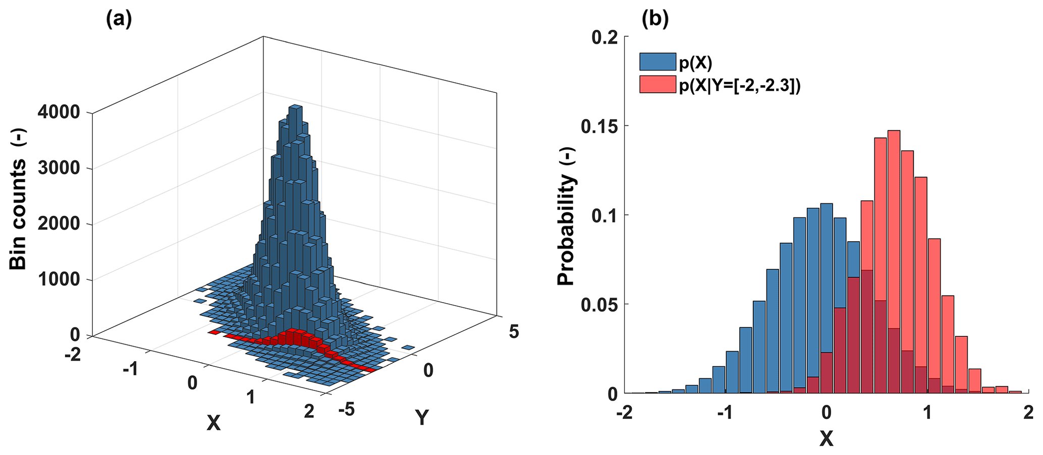
Figure 1Illustration of a bivariate conditional probability distribution as a simple data-based predictive model. (a) Joint histogram of target X and predictor Y (blue). Conditional histogram of target X given predictor values from the interval [−2, −2.3] (red). (b) Marginal (unconditional) probability distribution of target X (blue) and conditional probability distribution of target X given predictor values from the interval [−2, −2.3] (red).

Download

So far we have used entropy to measure uncertainty as if we have had to guess all values of a data tuple randomly drawn from an a priori known distribution. However, often we do not only know the distribution a priori, but we also have knowledge of the values of parts of the data tuples (e.g., we know Z and the empirical Z–R relation and want to predict R). In this case, our uncertainty regarding the target variate R given the predictor variate Z and the relation among the two can be measured by conditional entropy, which we know from Eq. (4) is always smaller than or equal to the unconditional entropy of the target. In Fig. 1a, the conditional frequency distribution of the target X given predictor Y is shown in red; in Fig. 1b, the related conditional probability distribution,also in red, and the unconditional probability distribution of the target, in blue, are shown.

In short, we can consider a dpd constructed from a data set as a “minimalistic predictive model”, which, given some values for the predictor variates, provides a probabilistic prediction of the target variate. It is minimalistic in the sense that it involves only a small number of assumptions (representativeness of the dpd) and user decisions (choice of the binning scheme). Compared with more common modeling approaches, where relations among data are expressed by deterministic equations, the advantage of a dpd-based model is that it yields probabilistic predictions in the form of conditional dpd's, which include a statement about the target value and the uncertainty associated with that statement. Also, as dpd-based modeling does not involve strong regularizations, it reduces the risk of introducing incorrect information. When building a standard model, choosing a particular deterministic equation to represent a data relation, which is a common form of regularization, involves the risk of introducing bias, and it ignores predictive uncertainty. In this context, Todini (2007) provides a very comprehensive discussion on the relative merits and problems of data-based models and models relying on additional information in the form of physical knowledge, as well as the role and treatment of predictive uncertainty.

Things are different, however, if we apply the model to a new situation, i.e., if we construct the model from one data set and use it with predictor data of another under the assumption that the predictor–target relation expressed by the model also holds for the new situation. This is clearly only the case if the learning and the application situation are identical; however, in most cases the situations will differ and we will pay for this inconsistency with additional uncertainty. We can measure this uncertainty using the Kullback–Leibler divergence (Eq. 6) between the dpd we use as a model and the true dpd of the application situation. Total predictive uncertainty is then expressed by cross entropy (Eq. 5) and can be calculated as the sum of the predictive uncertainty given a perfect model (expressed by conditional entropy), which is limited by the amount of information the predictors contain about the target and by the inadequacy of the model (expressed by Kullback–Leibler divergence).

We will apply this approach to construct and analyze predictive models throughout the paper, and use it to learn about the information content of various predictors about our target, ground rainfall R, and learn about the information losses when applying predictive models that were, e.g., constructed from limited data sets, constructed at different places, or simplified by functional compression. Note that expressing relations among predictor and target data by dpd's is not limited to data-based models, in fact functional relationships of any kind (e.g., the Marshall–Palmer Z–R relation) can be expressed in a dpd. In that sense, the framework for model building and testing as well as the measures to quantify uncertainty that we use here are universally applicable.

2.3 Data

This study uses data from various sources collected during a 4-year period (1 October 2012–30 September 2016) within the CAOS (Catchments As Organised Systems) research project. For more detail on project goals and partners see Zehe et al. (2014). QPE was an important component of CAOS, and to this end special focus was on measuring rain rates and drop size distributions (DSD) using six laser optical disdrometers, two vertical pointing K-band micro rain radars, standard rain gauges and weather radar. Table 1 provides an overview of these and additionally used data.

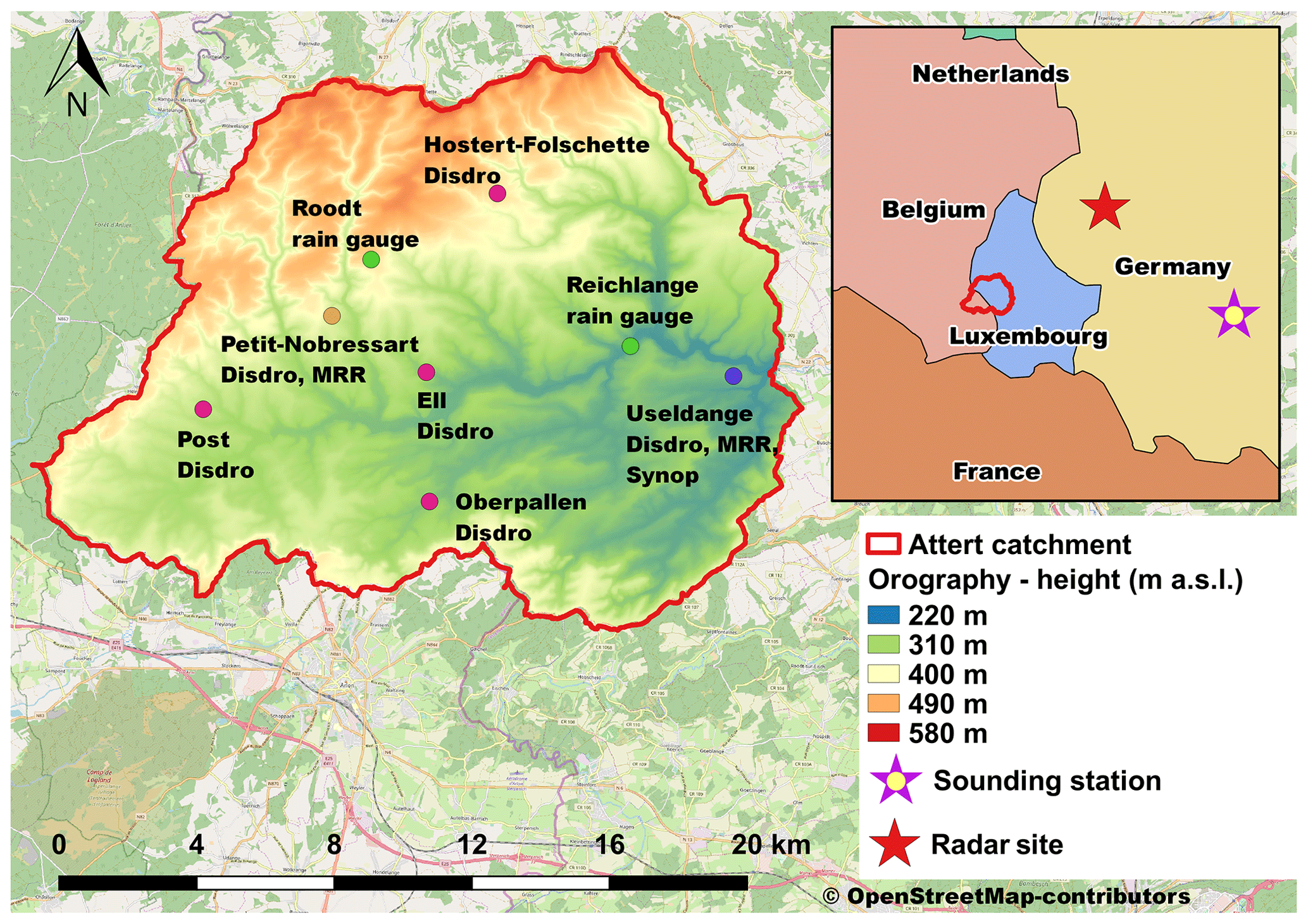
Figure 2The position of the Attert catchment in Luxembourg and Belgium with superimposed orography (in m a.s.l.) and the locations of the MRR's, disdrometers, rain gauges, the synoptic station (ASTA) and radar site (Neuheilenbach), and the rawinsonde launching (sounding) station (Idar-Oberstein – WMO-ID 10618) as well as the scale and orientation of the small-scale map. © OpenStreetMap contributors 2019. Distributed under a Creative Commons BY-SA License.

Table 1Summary of the raw data used in the experiments: description, summary statistics and binning.

^a [min, max]; ^b [center of first bin, uniform bin width, center of last bin] number of bins; ^c 1: Ell, 2: Hostert–Folschette, 3: Oberpallen, 4: Petit-Nobressart, 5: Post, 6: Useldange, 7: Reichlange, 8: Roodt; + irregular binning with edges [−0.1 0.19 1 2 4 6 8 10 15 20 25 30 40 50 60 70 90 110 130]; $++$ irregular binning with edges [−100 11.5 23 27.8 32.6 35.5 37.5 39 41.8 43.8 45.4 46.6 48.6 50.2 51.5 52.5 54.3 55.7 56.8].

Download Print Version | Download XLSX

2.3.8 Data filter

Rainfall is an intermittent process, and quite expectedly most of our 4-year series contained zeroes for rainfall. If we had used this complete data set for analysis, the results would have been dominated by these dry cases; however, these cases were not what we were interested in. Therefore, we applied a data filter to select only the hydro-meteorologically relevant cases with measurements from all available stations and at least two rain gauges showing rainfall ≥ 0.5 mm h⁻¹. Additionally, cases with solid precipitation were excluded using the output from the disdrometers' present weather sensor software. In total, 11 984 data sets passed this “minimum precipitation” filter, which amounts to almost 17 months of hourly data.

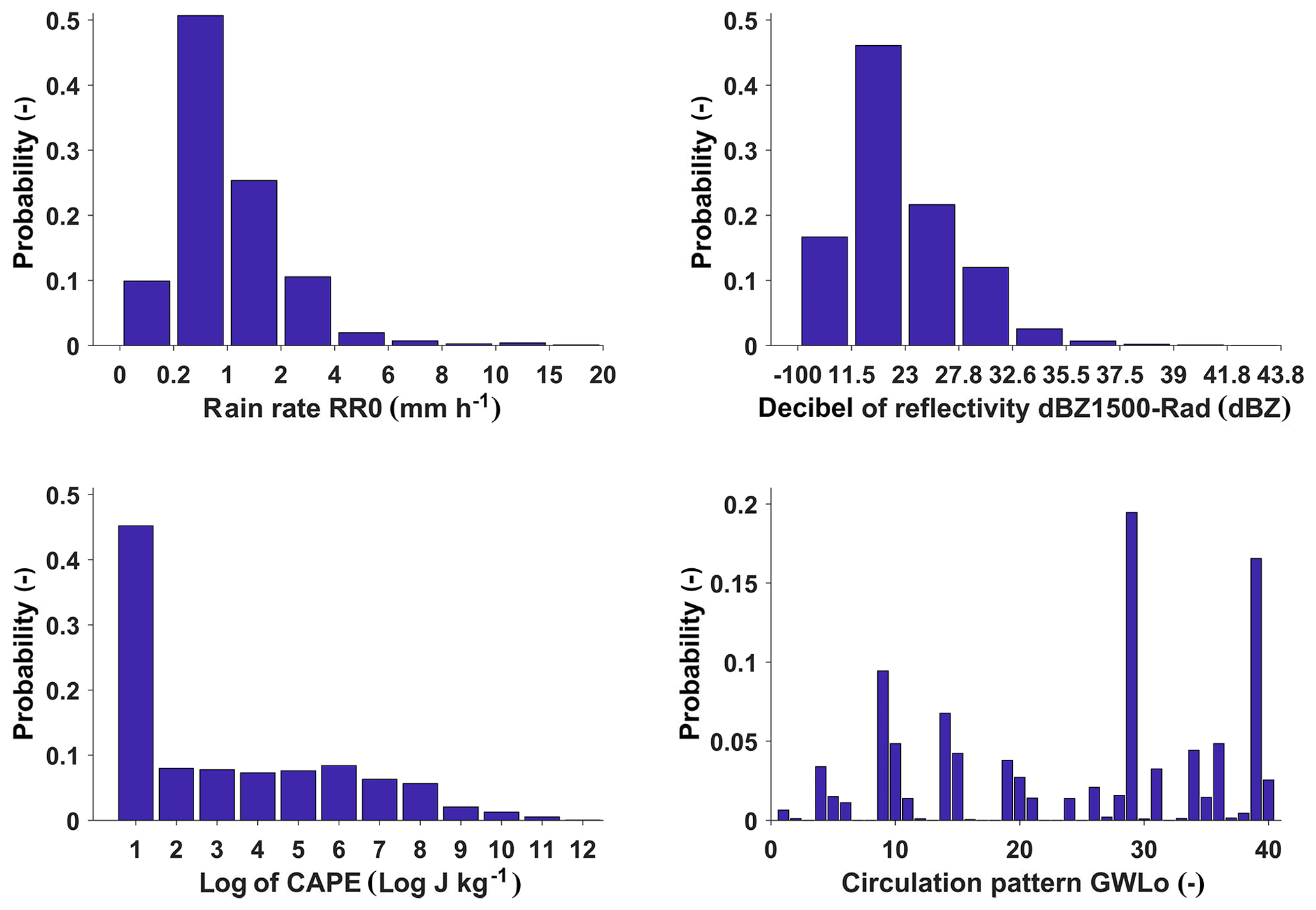
In Fig. 3, for the filtered data binned probability distributions of the most important variables are shown.

Figure 3Discrete probability distributions of the most important variables used in the experiments (filtered data set). The description of variables and binning can be found in Table 1. The x axes for rain rate and reflectivity are truncated on the right to avoid displaying empty bins.

Download

3.1 Experiment 1: information in various predictors

In this experiment we explore the information content regarding ground rainfall R in various predictors (see Table 1). We selected the predictors with the constraint that they are operationally available at any potential point of interest, which applies most importantly to reflectivity measured by weather radar, but also to the predictors we assumed to be spatially invariant within the test domain: convective available potential energy (as surface based CAPE), circulation pattern, air temperature and humidity, wind, and season. We excluded reflectivity measurements by MRR and disdrometer, as these are usually only available at a few locations.

We used ground rainfall observations from the eight rain gauges in the test domain as target data, filtered the raw data with the “minimum precipitation” filter and created models using various predictor combinations. We measured the usefulness of the predictors with entropy and conditional entropy (Eqs. 2 and 3). The results are shown in Table 2.

Table 2Entropy of the target (RR0) and the benchmark distribution (RR0 uniform), conditional entropies of the target given one or several predictors, non-normalized and normalized. Underlying data are from the filtered data set. Predictors are ordered by descending conditional entropy.

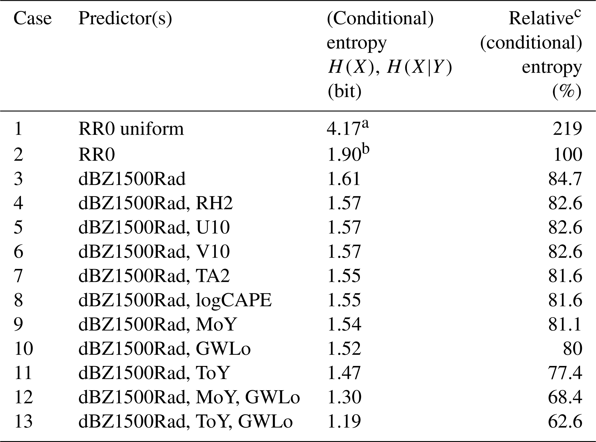
^a Unconditional entropy of the benchmark uniform distribution; ^b Unconditional entropy of the target; ^c H(RR0|predictor(s))∕H(RR0) ⋅ 100.

Download Print Version | Download XLSX

There are two upper benchmarks we can use to compare the different QPE models against: unconditional entropy if we know nothing but the binning of the target and use a uniform (maximum entropy) distribution for prediction (case 1 in Table 2), and the unconditional entropy of the observed distribution of the target (case 2 in Table 2), which we used as a reference here. The difference between the two is considerable (119 %), which means that merely knowing the true distribution of RR0 is already a valuable source of information.

The next important source of information is radar reflectivities: if we use it as a single predictor (case 3), uncertainty is reduced by 0.28 bit or 15.3 % compared with RR0. Note that this approach directly applies the reflectivity data provided by the radar, no side information was added nor existing information in the data destroyed by applying an additional Z–R relation. This result shows, on the one hand, that radar reflectivity is one of the most important sources of information. On the other hand – as the reduction in uncertainty is quite low when RR0 is conditioned by dBZ1500Rad – the high variability in the Z–R relationship limits entropy reduction. The may be due in part to the effects of the vertical profile of reflectivity and attenuation at high rain rates.

Using each of the other predictors separately did not reduce uncertainty much (not shown); therefore, we only show results for the cases where they were applied as two-predictor models in combination with radar reflectivity (cases 4 to 11). If we compare the relative conditional entropies of their predictions to those of the radar-only model, we can see that neither the ground meteorological observations nor CAPE contained much additional information (cases 4 to 8). Instead, the three most informative models (cases 9 to 11) either distinguish the relation between R and Z by circulation pattern or by season, which corresponds to the operational practice of many weather services to use one Z–R relation for summer and one for winter.

Based on these results, we built and evaluated three-predictor models only with combinations of these relatively informative predictors (cases 12 and 13). The information gain from using three predictors in combination is considerable, and it reduced uncertainty to 68.4 % (case 12) and 62.6 % (case 13) compared with the “target-distribution-only case” (case 2). The benefit of applying a season-dependent and circulation-pattern-dependent relation between R and Z also becomes obvious if we compare case 3 (the radar-only model) with cases 12 and 13: in the first case, uncertainty is reduced by 16.3 %, in the latter by 22.1 %.

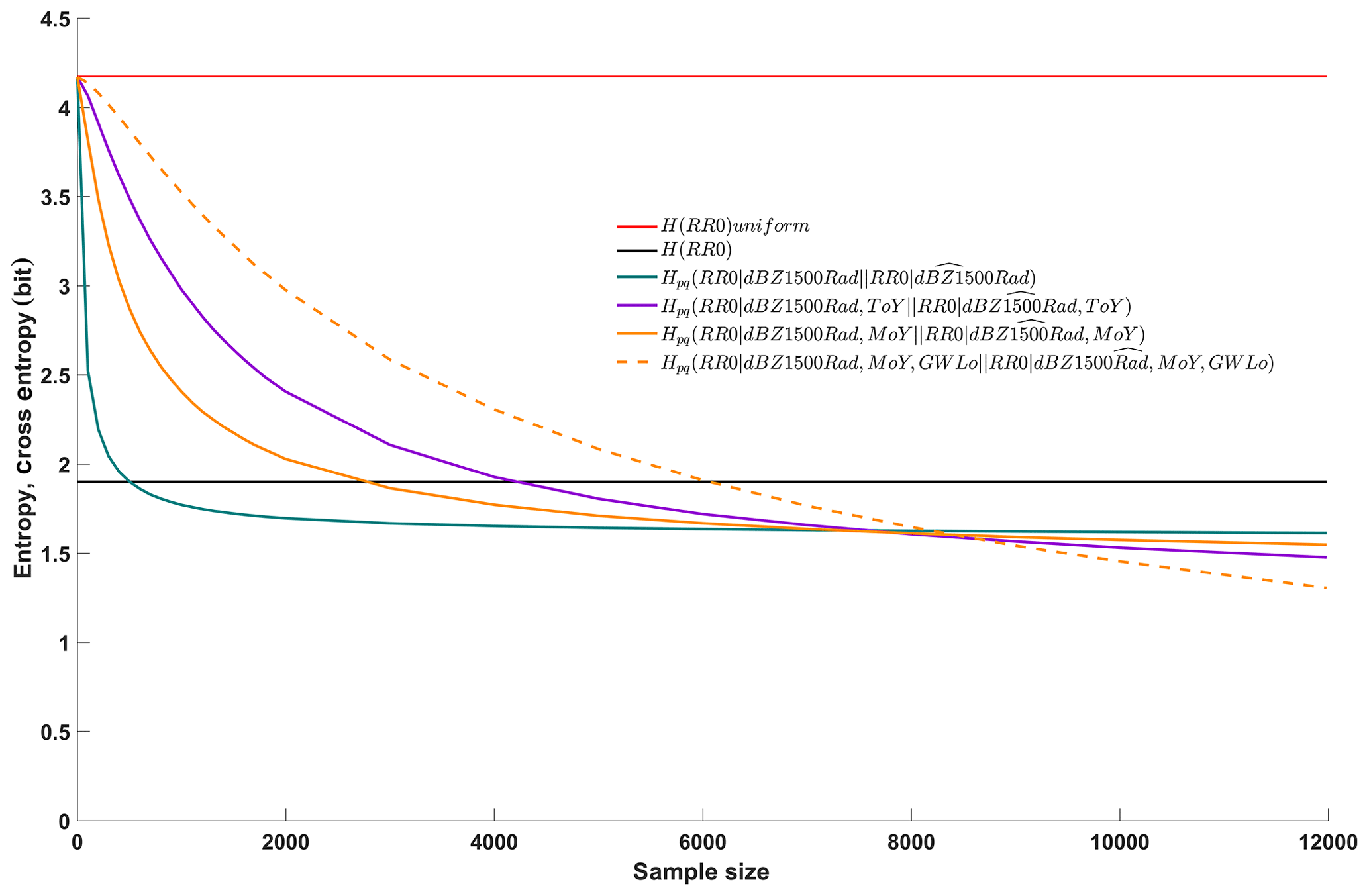
Figure 4Entropy of the unconditional target distribution (filtered data set, black line), entropy of the benchmark uniform distribution (filtered data set, red line), cross entropies between conditional distributions of the target given one, two and three predictors of the filtered data set and samples thereof (green, purple, yellow and dashed yellow lines, respectively). The “∧” symbol indicates a sample.

Download

An obvious conclusion from these findings would be to build better models by simply adding more predictors, which according to the information inequality equation (Eq. 4) never hurts. In fact, when learning from limited data sets, adding enough predictors will, in the end, result in perfect models with zero predictive uncertainty. However, there is a catch to this, which is known as overfitting: in order for a model to be robust in the sense of “being only weakly sensitive to the presence or absence of particular observations in the learning data set” and “performing well not only within the training data set, but also on data unseen during training”, it must be supported by an adequate number of learning data, and this number grows exponentially with the number of predictors included in the model. So instead of adding more predictors, we will explore the robustness of our models in the next experiment.

3.2 Experiment 2: the effect of sample size

The data base and filter used here are identical to the previous experiment, so a set of 11 984 joint observations of the target (rain rate at the ground) and predictors (radar reflectivity, circulation pattern, tenner-day and month of the year) were available. From these data we built and tested a total of four predictive models, as described in Experiment 1: a one-predictor model applying radar reflectivity only, two two-predictor models applying radar reflectivity and tenner-day or month of the year, and a three-predictor model using radar reflectivity, month of the year and circulation pattern. The difference to Experiment 1 is that we now do not only apply the entire data set but also randomly drawn samples thereof to build the model (see Sect. 2.2 for an explanation of the sampling strategy). Each model is then applied to and evaluated against the full data set. In this case, total predictive uncertainty is measured by cross entropy (Eq. 5), which is the sum of conditional entropy of the target given the predictors for the full data set and Kullback–Leibler divergence of the sample-based model and the model built from the full data set (see Sect. 2.2).

The results are shown in Fig. 4 as a function of sample size. As in Experiment 1, we included the benchmark uncertainties for applying a maximum entropy model (red horizontal line, case 1 in Table 2) and a zero-predictor model (black horizontal line, case 2 in Table 2) to put the other models into perspective.

On the right margin of Fig. 4, cross entropies are shown for the case where the sample comprises the entire data set. In this case, Kullback–Leibler divergence is zero, and total uncertainty equals conditional entropy. This is the same situation as in Experiment 1, and the values correspond to those in Table 2 for cases 3, 9, 10 and 12. The three-predictor model (dashed yellow line) quite expectedly outperforms the two-predictor models (solid purple and yellow lines), which in turn outperform the one-predictor model (solid green line). However, things look different if only samples are used for learning. With respect to the one-predictor model, for very small sample sizes close to zero, the information content of the sample is close to zero; hence, the predictive uncertainty is close to that of the ignorant maximum entropy model (red line) and considerably higher than that of the zero-predictor model. However, when increasing the size of the sample just a little, its information content quickly rises and cross entropy drops. In fact, when learning the relation between radar reflectivity and ground rainfall from only about 2000 joint observations, the model is almost identical to a model learned from the full data set of 11 984 joint observations: Kullback–Leibler divergence is almost zero and cross entropy is almost as low as for the model built from the full data set. From this we can conclude that the full data set contains considerable redundancy, which in turn implies that we can build robust one-predictor models from the available data.

We can interpret the lines in Fig. 4 as learning curves, or more specifically they represent the information about the target contained in samples of different sizes. If we now consider the two two-predictor models and the three-predictor model and compare them to the one-predictor model, we can see that the more predictors we add, the slower the learning rates become and the longer learning takes (the curve inclinations are lower for small sample sizes, but remain nonzero for larger samples). For the two two-predictor models this means that samples larger than about 8000 (about two-thirds of the data set) are required before their total predictive uncertainties fall below that of the one-predictor model. For the three-predictor model, even samples larger than about 8500 are required, and the model interestingly continues to learn even for very large sample sizes (the yellow dashed line is still inclined, even for large samples).

The learning behavior of the models, which differs with the number of predictors used, is a manifestation of the “curse of dimensionality”, and visual examination of learning curves of different models as plotted in Fig. 4 allows two choices: for a given sample size, we can choose the best (least uncertain) model; for a given size data set, we can choose the model with the best trade-off between performance and robustness. For the latter choice, we can establish selection criteria such as “a model qualifies as robust if it learns from at maximum of two-thirds of the available data at least 95 % of what it can learn from the entire data set” and then choose the best model satisfying this criterion. From the models displayed here, according to our subjective choice, the two-predictor model using a month-specific relation between radar reflectivity and ground rainfall provides the best trade-off between performance and robustness.

3.3 Experiment 3: site-specific Z–R relations

In this experiment we investigate the information content in spatial position by learning and applying site-specific relations between radar reflectivity and ground rain rate (in the previous experiments we applied them in a spatially pooled manner). We used data filtered with the “minimum precipitation” filter again, so a set of 11 984 joint observations of ground rain rate and radar reflectivity were available. We included spatial information by simply using the ID number of each station (“Statnum” in Table 1) as an additional predictor, which means that we built and applied relations between reflectivity and rain rate at the ground specifically for each station in the test domain (see Fig. 2). As in the previous experiment, we evaluated the predictive performance of these models as a function of sample size with cross entropy. The results are shown in Fig. 5.

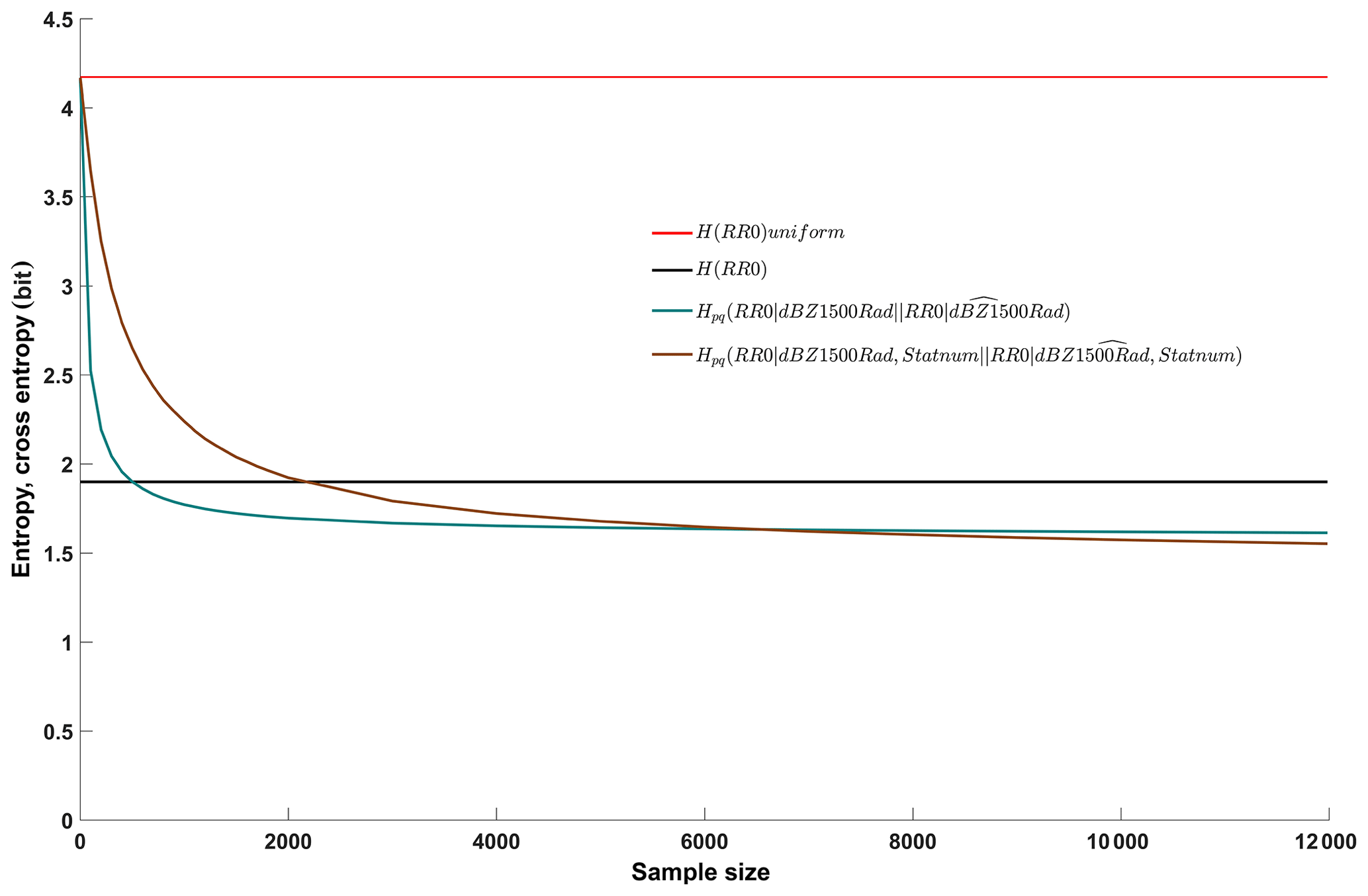
Figure 5Entropy of the unconditional, target distribution (filtered data set, black line, same as in Fig. 4), entropy of the benchmark uniform distribution (filtered data set, red line, same as in Fig. 4), cross entropies between conditional distributions of the target of the filtered data set and samples thereof: one-predictor model applying dBZ1500Rad (green line, same as in Fig. 4), two-predictor model applying dBZ1500Rad and station number (brown line). The “∧” symbol indicates a sample.

Download

The red and black horizontal lines are the same as in Fig. 4 and (as previously) represent the benchmark unconditional entropies of the target for a maximum entropy uniform distribution and the observed distribution. A green line was also included in Fig. 4 and represents the conditional entropy of the one-predictor model applying radar reflectivity only. The brown line shows the performance of the two-predictor model including the station ID. The overall pattern is similar to Experiment 2: adding a predictor reduces the total uncertainty if the full data set is used for learning (at the right margin, the brown line lies below the green), but higher-predictor models require more data for learning (the green line descends more slowly and over a longer period than the brown). Here, the two-predictor model outperforms the zero-predictor model only for samples larger than 2200, and the one-predictor model only for samples larger than 6500.

Overall, the information gain of using site-specific Z–R relations is moderate (cross entropy of the radar-only model for the full data set is 1.61 bit, whereas it is 1.55 bit for the site-specific model) and lower than when distinguishing Z–R relations according to time or circulation pattern (cases 9, 10 and 11 in Table 2). This is not very surprising if we consider the extent of the test domain: the largest distance between two stations is 9.5 km (between Oberpallen and Useldange stations), and the largest elevation difference is 182 m (between Reichlange and Roodt stations). Across these relatively small distances, it appears reasonable that Z–R relations do not differ substantially. However, this could be different when working in larger domains or in domains with hydro-meteorologically distinctly different subdomains, such as lowlands and mountain areas or different climate zones (as shown, for example, in Diem, 1968).

3.4 Experiment 4: the effect of functional compression

In this experiment we evaluate the effect of functional compression by measuring the information loss when using a deterministic function to express the relation between radar reflectivity and ground rain rate instead of the empirical relation derived from the data. As before, we used all joint observations of radar reflectivity and ground rainfall passing the “minimum precipitation” filter. Each data pair is shown as a blue dot in Fig. 6, and we can see that a strong, positive and nonlinear relation exists between them. We already made use of this relation in Experiment 1 when we built a one-predictor model using reflectivity to estimate ground rainfall. Comparing cases 2 and 3 in Table 2 we can see that prior knowledge of reflectivity indeed contains valuable information, reducing total uncertainty by 15.3 % (100 % to 84.7 %).

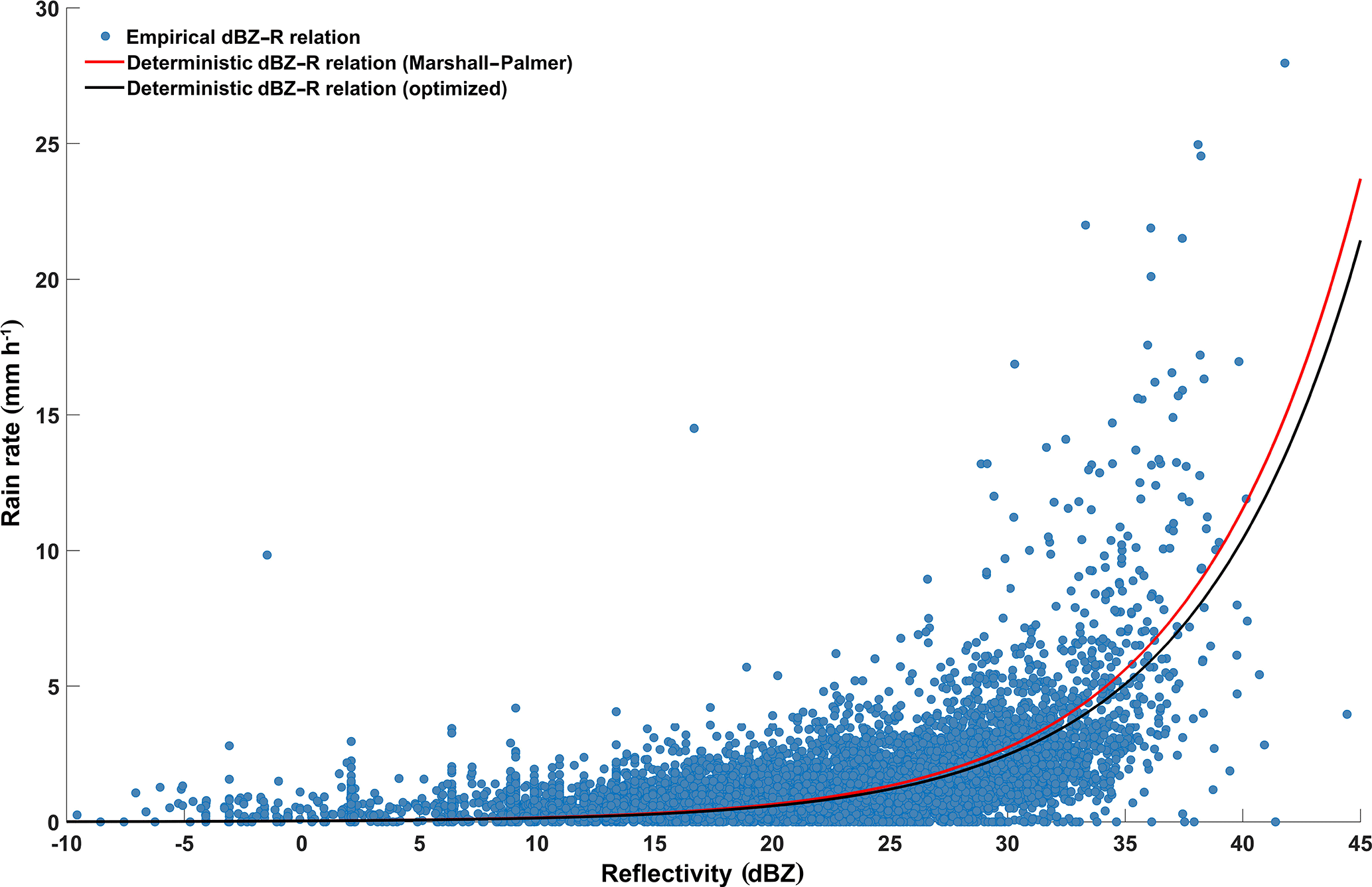
Figure 6Relation between target RR0 and predictor dBZ1500Rad. Empirical relation as given by the filtered data set (blue dots). Deterministic power-law relation according to Marshall and Palmer (1948) (red line); deterministic power-law relation with optimized parameters a=235 and b=1.6 (black line).

Download

Let us suppose we would not have been in the comfortable situation of having joint observations of target and predictor to construct a data-based model, or suppose it would take too much storage or computational resources to either store or apply such a model. In these cases, it could be reasonable to approximate the “scattered” relation as contained in the data either using a deterministic function gained from other data or a deterministic function fitted to the data. In fact, this is standard practice. Expressing a data relation by a function drastically reduces storage space, is easy to apply and preserves the overall relation among the data. However, what we lose is information about the strength of that relation as expressed by the scatter of the data. Instead, when applying a deterministic function we claim that the predictive uncertainty of the target is zero.

Our aim here is to quantify the information loss associated with such deterministic functional compression. Applying a deterministic model is in principle no different than using a model learned from a subset of the data, as we did in Experiment 2: we use an imperfect model, which results in additional uncertainty which we can measure via Kullback–Leibler divergence between the true data relation and the model we apply (see Eq. 6). Total predictive uncertainty is then measured by cross entropy (Eq. 5) as the sum of conditional entropy (the uncertainty due to incomplete information of the predictor about the target) and Kullback–Leibler divergence (see Sect. 2.2).

For demonstration purposes we applied two typical deterministic Z–R relations of the form $Z=a\cdot R^b$. The first is the widely used Marshall–Palmer relation (mostly attributed to Marshall and Palmer (1948) as, for example, in Battan (1959b) and Sauvageot (1992); however, the origin of this particular formula is unknown to the authors) with parameters a=200 and b=1.6. The Marshall–Palmer relation is often used as a default model if no better options or local data are available. For the second, we assumed the local reflectivity and rain rate observations to be available and used them to optimize parameter a by minimizing the root mean square error (RMSE) between the observed rain rate and the modeled rain rate using reflectivity observations. Following the recommendations by Hagen and Yuter (2003), we only varied a and kept b constant at 1.6. In the end, the optimized a=235 was not far from its Marshall–Palmer pendant and only reduced the RMSE slightly from 1.18 mm h⁻¹ (Marshall–Palmer relation) to 1.17 mm h⁻¹. Apparently, the default Marshall–Palmer relation already nicely fit our data. In Fig. 6, the two deterministic Z–R functions are plotted using red (Marshall–Palmer) and black (optimized Z–R relation) lines. Both capture the overall shape of the empirical Z–R relation quite well, except for high reflectivities where they tend to underestimate the observed rain rates. Applying such a deterministic Z–R relation to a given reflectivity observation is straightforward and yields a prediction of the related rain rate. However, from such a single-valued prediction we cannot infer the related predictive uncertainty, and the best we can do is to additionally provide the model's RMSE as a proxy.

As described above, we additionally used our information-based approach and calculated the conditional Kullback–Leibler divergence between the predictive distributions given by the empirical (perfect) and the deterministic (imperfect) models for all available data. From Eq. (6) we see that when comparing a reference distribution p to a model distribution q, a situation can occur where the latter is zero but the former is not, which means that an event is contained in the reference data that, according to the model, can never occur. In such a case the Kullback–Leibler divergence will be infinite, branding the model as completely inadequate. However, this verdict may seem too strict, e.g., if the model shows otherwise good agreement with reality, if we have reason to believe that the mismatch only occurred from a lack of opportunity due to a small data set rather than due to a principal mismatch of model and reference or, as in our case, if we know that we are using a deterministic approximation instead of the real data relation. In such cases, infinite divergence can be avoided by padding empty bins of the model distribution with small but nonzero probabilities, which we did by applying the minimally invasive maximum entropy approach suggested by Darscheid et al. (2018).

For our data, conditional Kullback–Leibler divergence for the Marshall–Palmer model was 3.43 bit, and it was 2.69 bit for the optimized model. Added to the conditional entropy of the empirical Z–R relation, this resulted in total predictive uncertainties of 5.04 and 4.30 bit, respectively. In terms of relative contributions, this means that 68 % (Marshall–Palmer) and 62.5 % (optimized model) of total uncertainty are due to deterministic functional compression. This is quite considerable, and even more so if we compare these results to the two benchmark cases in Table 2 (cases 1 and 2): even the default and safe-side model of applying a uniform distribution (case 1) involves smaller predictive uncertainty than the deterministic models. This seems counterintuitive at first when recalling the good visual agreement of the empirical and deterministic Z–R relations in Fig. 6. The reason for such large Kullback–Leibler divergences is the relatively high binning resolution for rain rate (Table 1) in combination with the way Kullback–Leibler divergence is computed: probability differences are calculated bin by bin and irrespective of probabilities in neighboring bins. This means that even a small over- or underestimation of a model, with an offset of the main probability mass by just one bin compared with observations can result in large divergence, which can, in the end, even exceed that of a prudent model spreading probability mass evenly over the data range. For the data used in this experiment, we assume that the agreement between deterministic model predictions and observations would quickly increase when coarse-graining the binning. This would be an interesting question to pursue in a future study, but for now we restrict ourselves to the main conclusion of this experiment: as long as learning about and application of data relations is carried out in the same data set, compression of probabilistic data relationships to deterministic functions will invariably increase uncertainty about the target. However, for the forward case, i.e., cases where there are no data available for learning but predictions are nevertheless required, application of robust deterministic relations capturing the essential relation between available predictors and the target is useful.

3.5 Experiment 5: information gains along the radar path

In this experiment we explore how the information content about ground rainfall in reflectivity observations is related to the measurement position along a vertical profile above the rain gauge, and how it is related to the measurement device. To this end, we used data from two sites, Petit-Nobressart and Useldange (see Fig. 2), where a range of reflectivity observations along a 1500 m vertical profile starting at ground level was available: disdrometer observations of reflectivity and rain rate at ground level, MRR reflectivity observations at a 100 m resolution between 100 and 1500 m above ground, and observations from C-band weather radar at 1500 m. With the goal in mind of providing guidance for the layout of future QPE sensor networks, we addressed the following questions: “are MRR observations at 1500 m more informative than weather radar observations taken at the same height?”; “how much information is gained if we use near-surface instead of elevated MRR observations, thus omitting the influence of the vertical profile of reflectivity?”; and finally “how much information is lost if we measure reflectivity instead of rainfall at ground level?”.

In contrast to the previous experiments, we were restricted to two (instead of eight) sites with MRR's installed. This made the application of the standard “minimum precipitation” filter (see Sect. 2.3) inappropriate. Thus, instead of filtering the raw data by at least two rain gauges showing rainfall ≥ 0.5 mm h⁻¹, we now applied this threshold separately to each of the sites. At Petit-Nobressart a total of 1241 data tuples passed the filter, at Useldange 612 data tuples passed the filter (Useldange began operation a year after Petit-Nobressart).

As in Experiment 1, we used entropy and conditional entropy to measure the information content of the available predictors and added the entropy of both a uniform and the observed distribution of ground rainfall as benchmarks. The results are shown in Table 3. As the results for the two stations are similar, we mainly discuss Petit-Nobressart in the following, moving from the remotest and presumably least informative predictor to the closest.

Table 3Entropy of the target (RR0) and the benchmark distribution (RR0 uniform), conditional entropies of the target given various predictors along the radar path, non-normalized and normalized, for Petit-Nobressart and Useldange, respectively. Underlying data are from the filtered data set. Predictors are ordered by decreasing distance to the target.

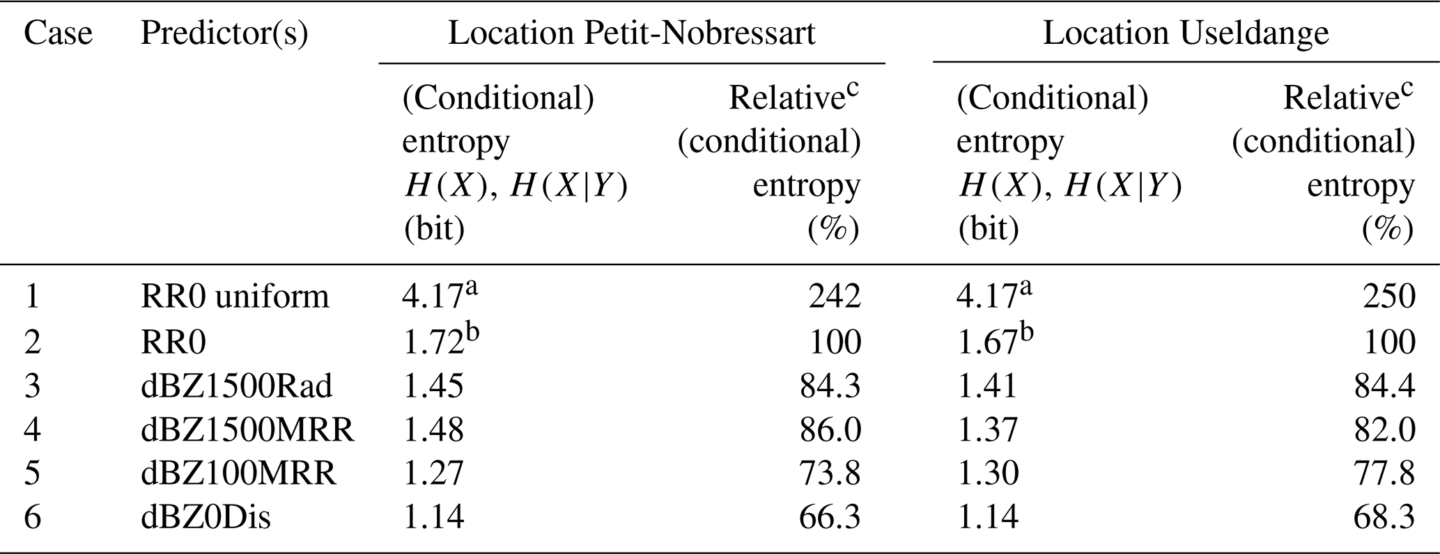
^a Unconditional entropy of the benchmark uniform distribution; ^b Unconditional entropy of the target; ^c H(RR0|predictor)∕(RR0) ⋅ 100.

Download Print Version | Download XLSX

Weather radar data, even if they are measured at distance and at height contain considerable information about ground rainfall: using them as predictors reduced uncertainty by 15.7 % (100 % to 84.3 %) compared with the benchmark entropy of the target distribution (Table 3, cases 2 and 3). This is comparable to the outcomes of Experiment 1 based on all sites (15.3 %, Table 2, same cases). We expected MRR observations taken at the same site and elevation to be more informative than their weather radar pendant, because the MRR signal path, and with it the potential for signal corruption, is considerably shorter. However, this is not clearly evident from the results: at Useldange the use of MRR instead of weather radar data additionally reduced uncertainty by only 2.4 % (84.4 % to 82.0 %, Table 3, cases 3 and 4), and at Petit-Nobressart they were even less informative (86.0 % instead of 84.4 %, Table 3, same cases). These results should be interpreted with some care due to the relatively limited data base; however, it seems safe to conclude that there is no large difference in the information content of MRR and weather radar observations taken at height.

So why go to the extra trouble of operating an MRR? The advantages of this instrument are evident when moving down to elevations inaccessible by weather radar. Changes in drop size distribution along the pathway of rainfall from cloud to ground can be considerable, and the closer to the ground the observation is taken the stronger its relation to ground rainfall: using MRR data from the lowermost bin (≤100 m above ground) reduced uncertainty by 12.2 % compared with using the uppermost bin (86.0 % to 73.8 %, Table 3, cases 4 and 5). This emphasizes the importance of VPR correction when using weather radar data (Vignal et al., 1999, 2000). Based on these results, an obvious next step would be to derive VPR corrections from the two MRRs and investigate the information gain when applied to other sites in the domain; however, for the sake of brevity, we leave this for future studies.

Further information gains can be achieved when measuring reflectivity directly at the ground: using the disdrometer measurements further reduced uncertainty by 7.5 % (73.8 % to 66.3 %, Table 3, cases 5 and 6), compared with the MRR observations. This gain is not only due to using ground observations, which completely excludes any negative VPR effects, but also because predictor and target data were observed at the same spot and by the same sensor. Seen from this perspective, it is surprising that considerable uncertainty still remains (66.3 % of the benchmark uncertainty, Table 3, cases 6 and 2), which must be attributed to the ambiguous relationship between radar reflectivity and rain rate due to the natural variability of drop size distribution.

3.6 Experiment 6: QPE based on radar and rain gauge data

In this final experiment we compare two methods of QPE, radar-based and rain-gauge-based, and additionally explore the benefits of jointly tapping both sources of information. As we were not dependent on the availability of MRR data as in the previous experiment, we could again make use of the full eight-site set of observations filtered with the “minimum precipitation” filter.

We used the same data-based approach of constructing empirical dpd's as a predictive model as in all previous experiments; the only difference between the three tested QPE models was the type of predictor used: for the radar-based QPE, we used weather radar observations at 1500 m above ground in a one-predictor model to predict ground rainfall at the same site. This is the same approach that we applied in Experiment 1. For the rain-gauge-based QPE, we built a one-predictor model based on a straightforward approach comparable to leave-one-out cross validation: each of the eight available stations (see Fig. 2 and Table 1) was once used as a target station, and observations from each of the remaining seven stations were used separately as predictors. This way we could calculate the information content in the predictor as a function of the distance between stations. Eight stations render a total of 56 unique station pairings; for our stations, the minimum, average and maximum distances were 1.9, 7.2 and 15.3 km, respectively. For later plotting, we binned the results in seven distance classes with a respective 2 km width and took averages within each bin. This is comparable to using range bins when calculating a semivariogram.

For the joint QPE model we extended the approach used for rain gauge interpolation to a two-predictor model: again each of the eight available stations was used once as a target station; however, in this case, not only were observations from each of the respective remaining stations used as predictors, but radar observations measured at height above the target station were also applied. This is a typical approach when merging radar and rain gauge data for QPE: we use data from rain gauges observed at a horizontal distance from the target, and radar data observed at a vertical distance from the target.

As we built and compared models with different numbers of predictors in this experiment, and as the models for each particular target station were built from a subset of the data only, it could be worthwhile exploring the additional uncertainty due to the effect of sample size here as in experiments 2 and 3. However, for this particular experiment we found it more useful for the reader (and us) to discuss results as a function of the distance between stations, as it provides a link to the large body of literature on spatial rainfall structure analysis and station-based rainfall interpolation. The results are shown in Fig. 7.

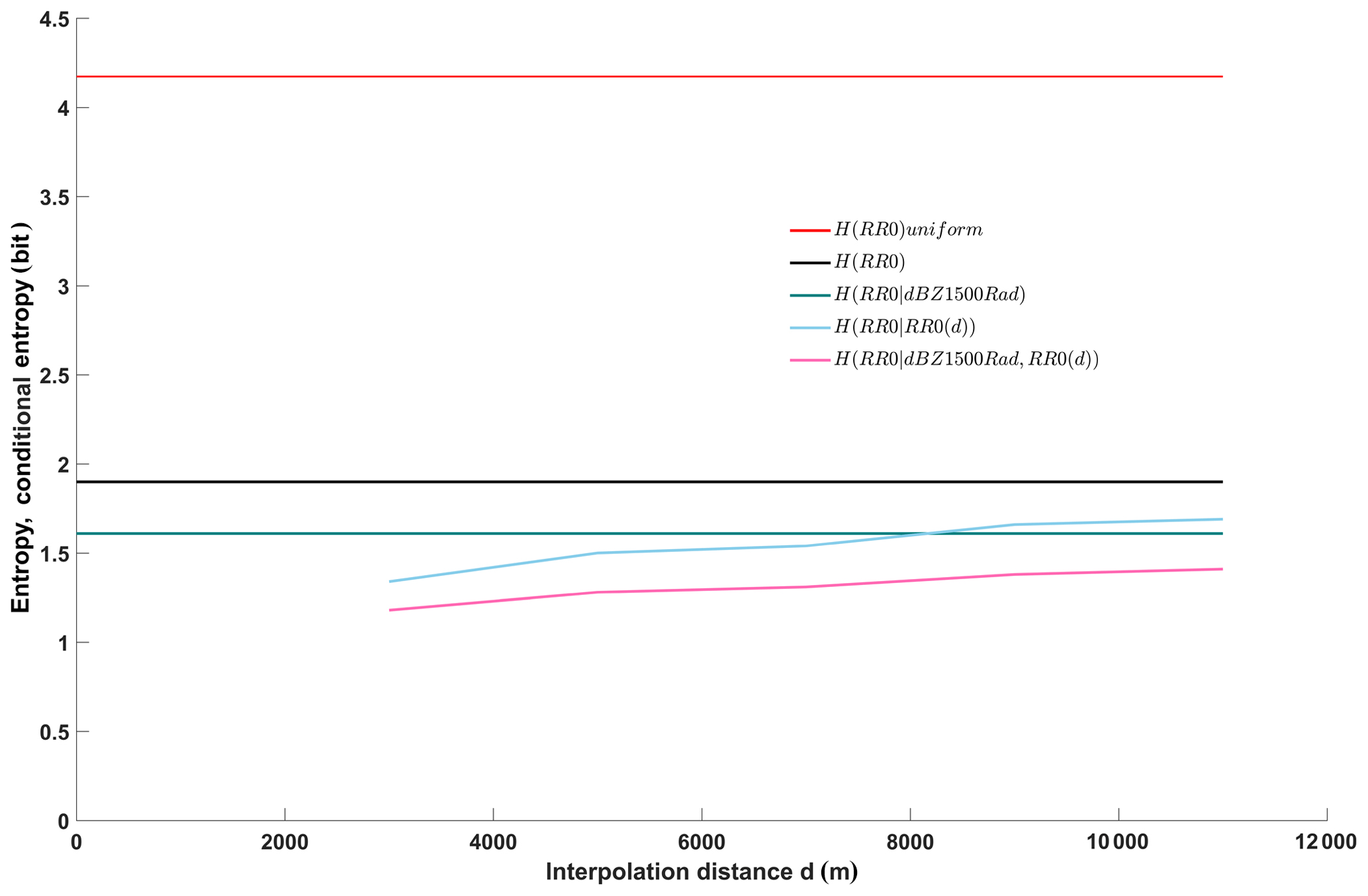
Figure 7Entropy of the unconditional, target distribution (filtered data set, black line, same as in Fig. 4); entropy of the benchmark uniform distribution (filtered data set, red line, same as in Fig. 4); conditional entropy of the target given reflectivity as predictor (green line); conditional entropy of the target given station rain rate observations as a function of interpolation distance (light blue line); and conditional entropy of the target given reflectivity and rain rate at stations as a predictor as a function of interpolation distance (pink line). Underlying data are from the filtered data set.

Download

Just as in Figs. 4 and 5, we included the benchmark unconditional entropies of the target for a maximum entropy uniform distribution (red line) and the observed distribution of all stations combined (black line) to put the results into perspective. As the radar-only model (green line) is independent of any interpolation distance, simply because it does not make use of any station data, it plots as a horizontal line. Its conditional entropy (1.61 bit) corresponds to the right-hand (full-size sample) value of the green line in Fig. 4, and to case 3 in Table 2.

However, for the QPE model based on rain gauge observations (light blue line), the interpolation distance does play a role: as is to be expected, the smaller the distance between the target and the predictor station, the higher the information content of the predictor and the smaller the conditional entropy, i.e., the blue line rises from left to right. For short distances between 2 and 4 km, conditional entropy is 1.34 bit, which is lower than for the radar-only QPE. If we take the unconditional entropy of the target again as a reference as in Experiment 1 (Table 1, case 2), station-only QPE for short distances reduces uncertainty to 70.5 %, and radar-only reduces uncertainty to 84.7 %. For long distances, however, this order is reversed, and station-only QPE only reduces uncertainty to 1.69 bit or 88.9 % of the reference. The break-even point at which both methods perform equally well lies at a station distance of about 8 km. This means that if we were asked to choose one of the two models for QPE, the best choice would be to use station interpolation for all targets within less than about 8 km from the nearest station, and radar-QPE for all others.

The above results indicate that each of the two QPE methods has its particular strengths. In other words they add nonredundant information; therefore, we can expect some benefits when joining them in a two-predictor model. This is indeed the case if we take a look at the related conditional entropies plotted as the pink line in Fig. 7. While it resembles the plot of the station-only model in overall shape and trend, it is shifted downward: conditional entropy for short distances is now reduced to only 1.18 bit (62.1 % of the reference), and even for the longest distances (1.41 bit = 74.2 % of the reference) it is still smaller than both the station-only and the radar-only values. Interestingly, in the combined model the radar observations add information – even for small station distances. We assume that this can be attributed to convective rainfall situations, where strong spatial rainfall heterogeneity occurs, unresolvable even by rain gauges only a few kilometers apart.

In Experiment 1 we also built and tested two-predictor models. The best among them, using radar data and tenner-days of the year for predictors (Table 1, case 11), reduced conditional entropy to 77.4 % of the reference. While this is a considerable improvement, it is surpassed by the radar–rain gauge model even for the largest station distance. Obviously, ground rainfall and radar observations contain nonredundant information which, when used together, have a large potential to improve QPE.