the Creative Commons Attribution 4.0 License.
the Creative Commons Attribution 4.0 License.
 | 22 Oct 2019
River-ice and water velocities using the Planet optical cubesat constellation
Bas Altena
Joseph Mascaro
The PlanetScope constellation consists of ∼150 optical cubesats that are evenly distributed like strings of pearls on two orbital planes, scanning the Earth's land surface once per day with an approximate spatial image resolution of 3 m. Subsequent cubesats on each of the orbital planes image the Earth surface with a nominal time lag of approximately 90 s between them, which produces near-simultaneous image pairs over the across-track overlaps of the cubesat swaths. We exploit this short time lag between subsequent Planet cubesat images to track river ice floes on northern rivers as indicators of water surface velocities. The method is demonstrated for a 60 km long reach of the Amur River in Siberia, and a 200 km long reach of the Yukon River in Alaska. The accuracy of the estimated horizontal surface velocities is of the order of ±0.01 m s−1. The application of our approach is complicated by cloud cover and low sun angles at high latitudes during the periods where rivers typically carry ice floes, and by the fact that the near-simultaneous swath overlaps, by design, do not cover the complete Earth surface. Still, the approach enables direct remote sensing of river surface velocities for numerous cold-region rivers at a number of locations and occasionally several times per year – which is much more frequent and over much larger areas than currently feasible. We find that freeze-up conditions seem to offer ice floes that are generally more suitable for tracking, and over longer time periods, compared with typical ice break-up conditions. The coverage of river velocities obtained could be particularly useful in combination with satellite measurements of river area, and river surface height and slope.


Knowledge about water surface velocities on rivers supports the understanding of a wide range of processes. In cold regions, river-ice freeze-up, and in particular break-up, and the associated transport of and action by ice debris is often the most important hydrological event of the year; this transport produces flood levels typically exceeding those of other periods (Fig. 1) and associated dramatic consequences for river ecology and infrastructure (e.g. Prowse et al., 2007; Kääb and Prowse, 2011; Rokaya et al., 2018a). River discharge measurements are complicated during freeze-up and break-up due to the physical impact of ice on instrumentation, and the determination of water surface speeds from tracking river ice floes can aid with estimating discharge (Beltaos and Kääb, 2014). This possibility is of particular importance for the major Arctic rivers of North America and Siberia, which transport large amounts of freshwater into the Arctic Ocean; however, the discharge of these rivers is least known for the ice break-up period – notably the period during which annual discharge peaks (Zakharova et al., 2019).
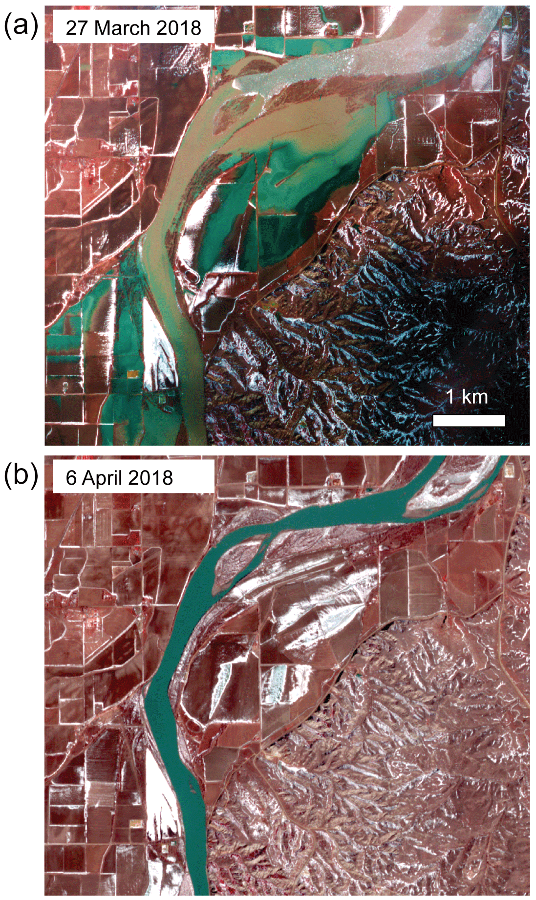
Figure 1Planet images over an ice jam on the Yellowstone River at Sidney, Nebraska, USA (47.75∘ N, 104.09∘ W). The river flows from bottom to top (north). (a) The ice jam (top) and associated flooding. (b) After break of the ice jam.
In addition to in situ measurements and ground-based remote sensing (e.g. Lin et al., 2019), water surface velocities are mainly retrieved using airborne or space-borne radar interferometry (Romeiser et al., 2007). During periods when rivers carry ice floes, or other visible surface objects, water velocities can be measured using near-simultaneous satellite (or airborne) images, optimally with time separations of the order of minutes (Kääb and Leprince, 2014). Such near-simultaneous imaging of the Earth surface is provided by satellite stereo sensors, where two or more stereo image partners are, by necessity, temporally separated by approximately 1–2 min (Kääb and Leprince, 2014). Ice floes (or other floating objects) are then tracked over this time lag to estimate water surface velocities during the image acquisition period. Satellite stereo imaging that is useful for this purpose stems from either fixed stereo or agile stereo. (In principle, satellite video could also be used to track ice floes but has to our knowledge not been demonstrated for this purpose yet; d'Angelo et al., 2014, 2016.) Fixed stereo is provided by two or more fixed cameras with different along-track viewing angles, e.g. the ASTER or ALOS PRISM sensors. Agile stereo is provided by one single camera that is rotated during overflight to point repeatedly to the same ground target, e.g. the WorldView or Pleiades satellites. Kääb and Prowse (2011) demonstrated the method deriving river-ice and water velocities over reaches of a few tens of kilometres of the Mackenzie and St. Lawrence rivers in Canada, using both types of satellite stereo images. Kääb et al. (2013) used ASTER fixed satellite stereo to measure and analyse river-ice flux and water velocities over a 600 km long reach of the Lena River in Siberia. Finally, Beltaos and Kääb (2014) demonstrated how water surface velocity fields derived in this way can be used to estimate river discharge. While Kääb and Leprince (2014) may have indicated other seasons and satellite constellations to track river ice floes over short time spans, all of the above studies have the following in common: (i) they use images during ice break-up for the most part, (ii) they use dedicated stereo systems, and (iii) they mostly use rare and opportunistic acquisitions. Point (i) limits the application of the method to one short time period of the year, and (ii) and in particular (iii) prevent the method from being applied operationally and systematically over large reaches of many rivers. The PlanetScope cubesat constellation offers the new, currently unexplored possibility of performing systematic worldwide observations of river-ice velocities and the water velocities indicated by them. The primary aim of the present study is to demonstrate and explore these possibilities, and the secondary aim is to evaluate the estimation of water velocities during river freeze-up, instead of during break-up. As the main focus of this study is a methodological one, we do not study the selected hydrological, hydraulic, or geomorphological applications that seem possible in detail.
The PlanetScope optical cubesat constellation scans the Earth surface systematically and daily (Figs. 2 and 3) involving the overlap of consecutive acquisitions with a time lag of around 1.5 min. A time lag of this order is perfectly suited to track floating matter, in particular river ice floes. Thus, PlanetScope offers the possibility of systematic daily measurement of water surface velocities, as long as ice floes are present on the water and sky conditions are clear. In this study, we first introduce the PlanetScope cubesat constellation in more detail. After a description of the methods used to track ice floes over minute-scale time lags, we demonstrate and discuss the typical ice-floe conditions suitable for tracking, and derive velocities over a 60 km long reach of the Amur River, Siberia, and a 200 km long reach of the Yukon River, Alaska. We also discuss the error budget of the measurements in detail. Finally, we draw conclusions regarding the potential for systematically measuring river-ice and water velocities from the PlanetScope constellation and briefly sketch out the possible fields for the application of this method.
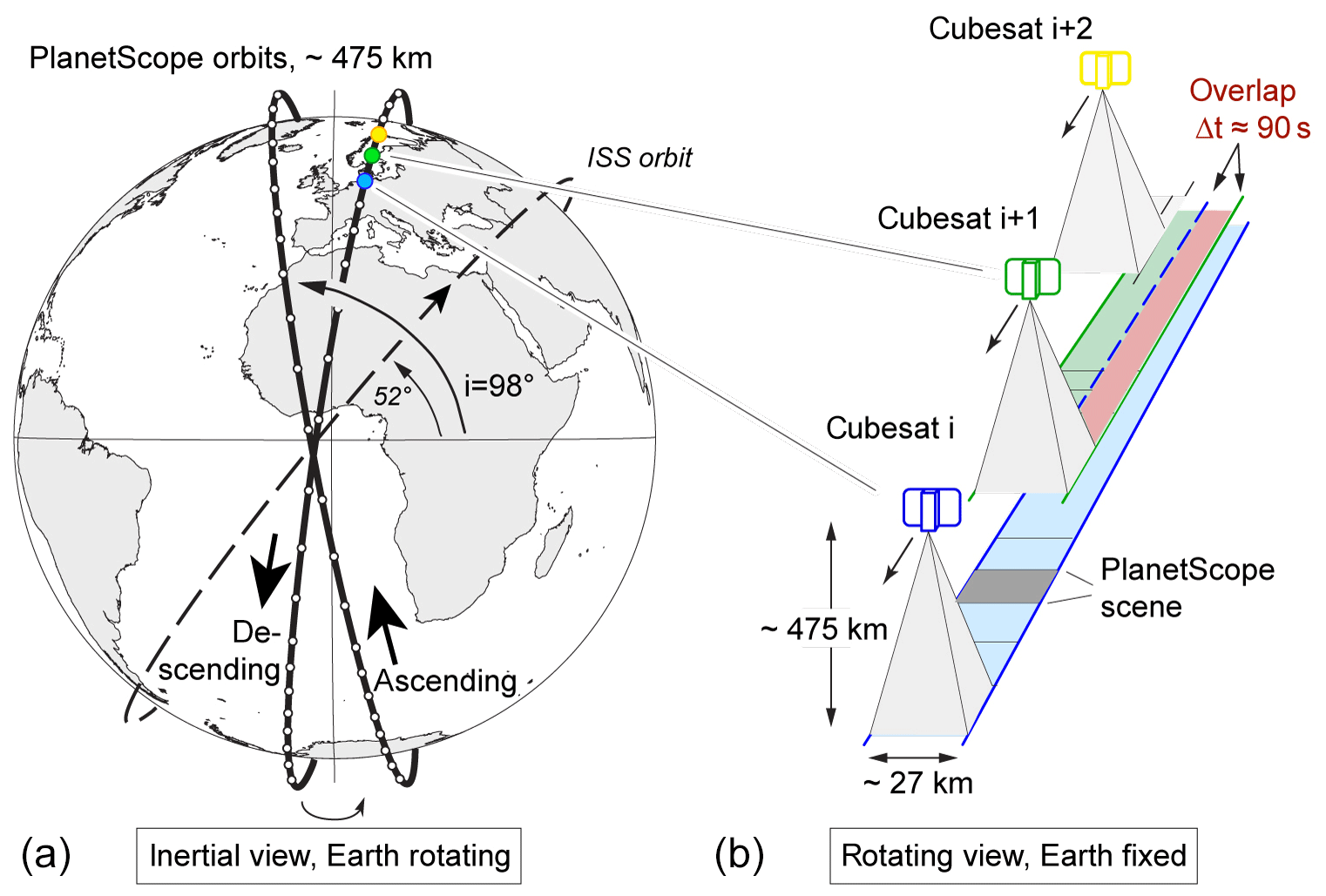
Figure 2Planet orbits. (a) Inertial view: the final PlanetScope descending and ascending orbits (bold) and the ISS test-bed orbit (dashed). Cubesat positions (white dots on the orbits) are only schematically indicated. (b) Rotating view: the complete scan scheme of the Earth surface by successive PlanetScope cubesats in the same orbit producing a time lag of around 90 s over the swath overlaps.
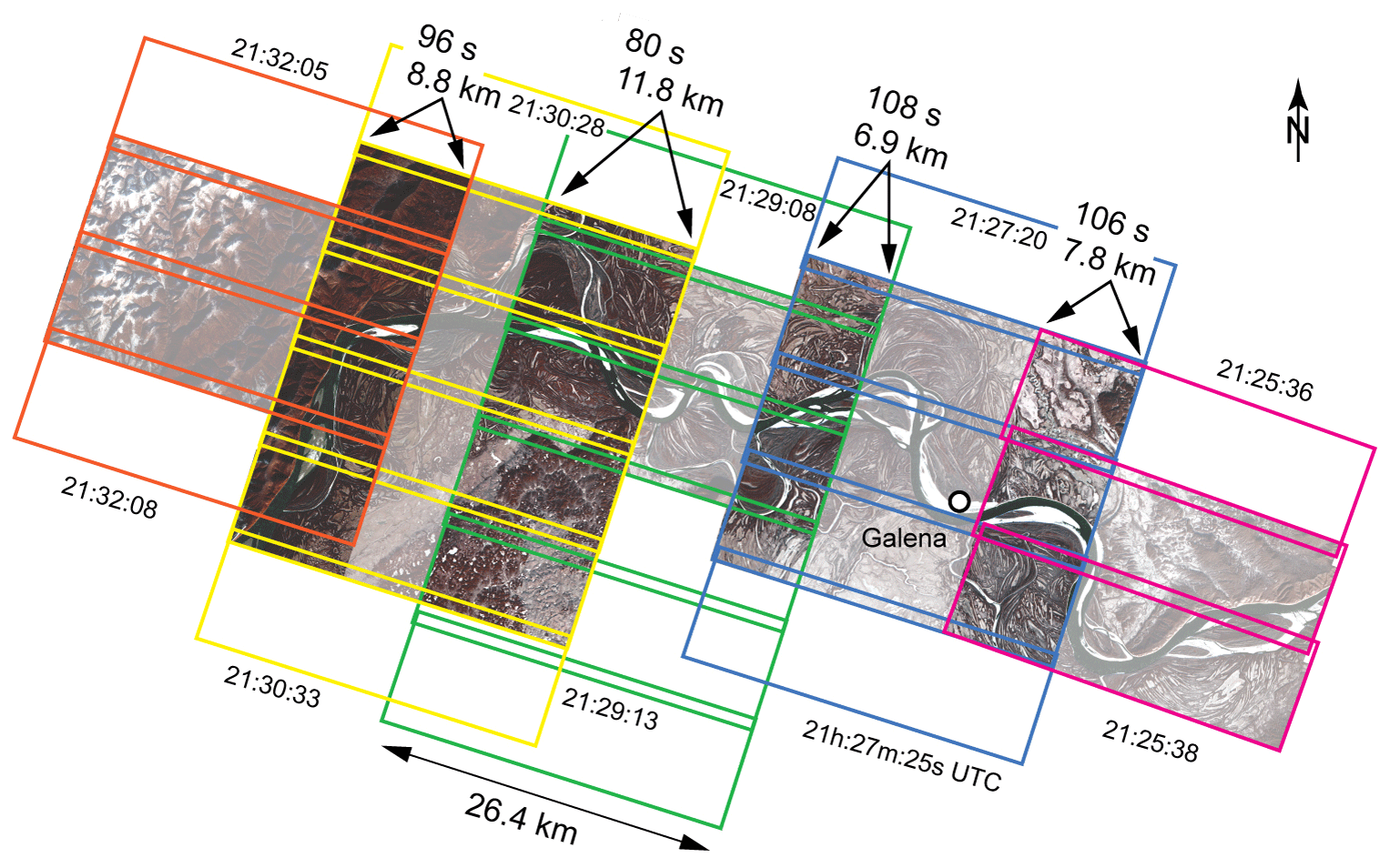
Figure 3Typical PlanetScope acquisition pattern on a cloud-free day during freeze-up (28 October 2018) over the Yukon River at Galena, Alaska (64.75∘ N, 157∘ W). Each colour indicates one satellite swath with individual scenes. Non-dimmed parts of the image indicate scene sections where two images with a time lag between them exist and river ice floes can be tracked. The time lag and width of the overlaps are given along with the time (UTC) of the acquisitions.
The following descriptions of the PlanetScope constellation and data, and the methods used, are an update and specification of the descriptions given by Kääb et al. (2017). The Planet cubesat constellation, referred to as PlanetScope, consists of small 10 cm × 10 cm × 30 cm satellites. Their main components are a telescope and CCD area array sensor. One half of the 6600 pixel × 4400 pixel CCD array acquires red–green–blue (RGB) data and the other half acquires near-infrared (NIR), both in 12 bit radiometric resolution. At the time of writing, the majority of the PlanetScope satellites provides images of about 3.7 m spatial resolution at an altitude of 475 km (delivered as resampled to 3 m; Fig. 1), and an individual scene size of roughly 25–30 km × 8–10 km (Planet Application Program Interface, 2019). While most other optical Earth observation instruments in space acquire in push-broom geometry (i.e. 1-D sensor arrays scanning in orbit direction), the data from the Planet satellites are 2-D frame images. Each complete image is taken at one single point in time, and has one single acquisition position and one single bundle of projection rays. For comparison, push-broom sensors integrate an image over a time interval of a few seconds so that acquisition time, position, and attitude angles vary throughout an image (Nuth and Kääb, 2011; Kääb et al., 2013; Girod et al., 2015).
Currently, the Planet cubesat constellation consists of around 150 cubesats following each other on two near-polar orbits of roughly 8 and 98∘ inclination respectively, and at an altitude of approximately 475 km (Fig. 2), imaging the Earth at local morning from both an ascending and descending orbit. The distance along the orbit between the cubesats is constructed such that the longitudinal progression between them over the rotating Earth leads to a void-less scan of the surface. Thus, the full constellation provides sun-synchronous coverage of the entire Earth (except the polar hole) with daily resolution (Fig. 2 in this paper ;Foster et al., 2015; Kääb et al., 2017). To guarantee this void-less surface imaging at all latitudes as well as when satellite positions and pointing angles are not exactly nominal, the swaths of subsequent cubesats overlap in the across-track direction by some kilometres (Figs. 2, 3). Within these swath-overlaps Earth surface targets are imaged twice (sometimes even more) with a time lag of roughly 1.5 min. This time lag is exploited in the present study and constitutes its core principle. The PlanetScope constellation also involves other time lags; however, these are not considered here (e.g. less than 1 s between RGB and NIR acquisitions; or a few hours, depending on the latitude, between acquisitions from ascending and descending orbits).
During the PlanetScope constellation's technological demonstration phase, the cubesats were mostly launched from the International Space Station into an orbit with a 52∘ inclination and an approximate 375 km height (Fig. 2 in this paper; Kääb et al., 2017). Data from these satellites form the majority of Planet's cubesat data archive holding for 2016 and into early 2017, before acquisitions from the near-polar sun-synchronous orbits took over. The build-up of the PlanetScope constellation and frequent replacement of its cubesats enables, among others, fast technological turnover and improvement of the image sensors. As a result, images from the more recent cubesat generations used in this study typically have better radiometric contrast than images from earlier generations.
Within the swath overlaps and over the corresponding approximate 1.5 min time lag we track river ice floes using standard image matching techniques. For image matching purposes, the geometric characteristics of repeat imagery are of particular interest. PlanetScope images are available at different processing levels, and here we use “analytic” data. Analytic data are radiometrically processed and orthorectified. We do not apply “unrectified” data, another processing level available, which comes with minimal radiometric processing and in the original central projection. The image orientation from on-board measurements is refined by Planet by matching the scenes onto a global reference mosaic (at the time of writing from Landsat, ALOS, and Open Street Map layers) and the images are orthoprojected using a digital elevation model (DEM). As for all orthoprojected satellite data, vertical errors in the orthorectification DEM cause lateral distortions in the resulting PlanetScope orthoimages. The size of these offsets is proportional to the DEM error and the off-nadir viewing angle (Kääb et al., 2016, 2017; Altena and Kääb, 2017). In a worst-case scenario for PlanetScope data (Kääb et al., 2017), a DEM error of 10 m results in orthorectification offsets of around 30 cm in the scene centre and 65 cm at the outer scene margin. For repeat river observations, the differential effect of these offsets can be reduced by co-registering the near-simultaneous images using stable points along shorelines. Over the limited width of rivers (a few kilometres at most), water surface topography is approximately planar. This means that a first-order polynomial co-registration model is sufficient to bring repeat unrectified frame images into overlap. This co-registration procedure will also greatly reduce offsets between the orthorectified analytic images used here, as the same DEM is used for both near-simultaneous images (Kääb et al., 2017). Errors in the DEMs used for orthorectifying PlanetScope images are a composite of (i) DEM elevation errors with respect to the real topography at the time of DEM acquisition, and of (ii) real-world elevation changes between the elevations at DEM acquisition and the elevations at satellite image acquisition. Orthorectification DEMs are, by necessity, outdated (although generally with limited consequences) unless acquired simultaneously with image acquisition. For river surfaces, the latter elevation deviations will primarily stem from water level variations between the DEM acquisition and the image acquisition dates. However, the small field of view of PlanetScope cubesats and the resulting low sensitivity to orthorectification DEM errors, the frame geometry of the PlanetScope cameras, and the accessibility of unrectified images, if needed, all contribute to minimize topographic distortions.
Bright ice floes on a dark water surface constitute features of strong visual contrast and tracking them over short time intervals is a particularly easy task for image matching algorithms. Thus, for matching the repeat PlanetScope data, we use a standard method – normalized cross-correlation (NCC) – solving the cross-correlation in the spatial domain and reaching sub-pixel accuracy by interpolation of the image (Kääb and Vollmer, 2000; Debella-Gilo and Kääb, 2011b; Kääb, 2014). NCC solves for translations between corresponding image elements. We apply the Correlation Image Analysis software (Kääb, 2014), but established scripts or routines for normalized cross-correlation between images exist for many programming languages. As the tracking of ice floes over short time intervals represents little challenge for image matching, we expect that other image matching methods (Heid and Kääb, 2012; Lin et al., 2019) would not provide a substantial advantage. However, over longer time intervals or strong horizontal water turbulence conditions, such as backwaters, ice-floe rotation over time would become significant; therefore, in these cases, image matching methods that are able to model feature rotation in addition to translation could be advantageous (Debella-Gilo and Kääb, 2012). The matching window sizes used in this study for the PlanetScope data are 30 pixels × 30 pixels (90 m × 90 m) as was found to be roughly optimal from a few tests. However, tests with different window sizes are not the focus of this study (Debella-Gilo and Kääb, 2011a). Measurements with a correlation coefficient smaller than 0.7 are removed and no other post-processing is applied (Kääb et al., 2017).
For comparing and supplementing our results based on Planet cubesats, we also use data from other satellites. A Landsat 8 scene from 16 September 2013 (i.e. ice-free conditions) is employed to automatically delineate the river water surface over the Yukon River study reach used in this work. Indexes used for the purpose of mapping water areas from multispectral satellite data are typically based on the reflectance contrast of water between blue (high reflectance) and near-infrared wavelengths (low reflectance) (McFeeters, 1996; Pekel et al., 2016). However, for our study site and conditions, we find that the contrast between the blue and thermal infrared Landsat bands is larger than the blue vs. infrared contrast due to a high suspended sediment concentration that increases the near-infrared reflectance and, thus, reduces the contrast to reflectance at blue wavelengths. To increase index sensitivity compared with the commonly used normalized difference indexes (McFeeters, 1996), we apply a band ratio. Thus, river outlines were obtained from a raster-to-vector conversion of a noise-filtered (3×3 median filter) and thresholded band ratio image (Paul et al., 2002) between the blue and thermal infrared bands of Landsat 8. The Landsat 8 blue band has 30 m spatial resolution, and the thermal infrared bands are also provided at a 30 m resolution, although they were originally taken at 60 m resolution.
For one of our Planet cubesat acquisition pairs over the Yukon River, a Sentinel-2 scene exists that was taken with a 1 h time difference. Sentinel-2 multispectral data have a spatial resolution of up to 10 m (Drusch et al., 2012; Kääb et al., 2016). We visually identified the position of a number of large ice floes corresponding between the Planet and Sentinel-2 images and measured the associated displacement along the river to estimate average velocities over the 1 h time period.
In order to compare the velocity retrieval from Planet cubesat data to a method used earlier for the same purpose we also measure short-term ice-floe displacements over the Yukon River reach from an Advanced Spaceborne Thermal Emission and Reflection Radiometer (ASTER) stereo strip. The ASTER fixed satellite stereo, taken at a 15 m spatial resolution and in near-infrared, implies a time lag of around 55 s between the two images of a stereo pair that can be exploited to track ice floes in a very similar fashion to the Planet cubesat images. The exact procedures, performance, and accuracies are presented in Kääb et al. (2013). As a speciality, satellite vibrations (so-called jitter) were modelled and corrected for when using the ASTER data. The results presented here for the Yukon River are based on a specially tasked ASTER acquisition, and have not been published before.
The river flow results of this study are presented as simple maps of measured velocity vectors or magnitudes, or as longitudinal profiles of water flow speed and derived parameters. For the latter we have to average the velocity vectors along the river reach. For that purpose, we move a running window, which is 4 km long in the reach direction and has infinite width, in 100 m steps along the mean direction of a study reach. The window length of 4 km and the step size of 100 m are experimentally chosen for our study sites to smooth the measurements substantially but at the same time leave enough detail.
At each window position, the number of measurement grid points within the river mask from Landsat 8 data as well as the average (or median) speeds and directions for the velocity measurements within the correlation threshold are computed. Dividing the number of grid elements within the river mask by the window length then gives an approximate river width for each step. This river width is then corrected for the deviation between the mean flow direction per window step against the overall mean direction of the river reach studied, essentially rotating the window at each step to align with the actual flow direction. (Note that other procedures exist that are more specialized for estimating river width when the flow vectors are not available; Allen and Pavelsky, 2018.) The surface area flux is then the multiplication of the average river speed and (corrected) width for each window step.
4.1 River-ice conditions
Figure 4 illustrates a small subset of the typical river-ice conditions in Planet images that are suitable for tracking ice floes or ice features, and estimating water velocities. During break-up we find predominantly smaller ice floes with very variable densities of ice-floe cover (Fig. 4b, d, f, h). During freeze-up we typically find bigger ice floes and a more equal distribution of ice-floe cover density over the river surface. This simple description of differences between freeze-up and break-up ice conditions is an overall and qualitative one based on a substantial, although visual, exploration of Planet archive holdings; however, a range of exceptions and natural variations to this description certainly exist. Our extensive searches in the Planet image archive clearly suggest that the ice conditions that are suitable for tracking are more constant over time during river freeze-up and they stretch over longer time periods (up to approximately several days or even a week) compared with break-up conditions. Break-up ice conditions that are suitable for tracking typically only last one or several ice pulses of a few days at most, and often just a day or two. This makes it more probable to acquire/find images of suitable ice conditions during freeze-up than during break-up. However, for the northernmost latitudes, the freeze-up period reaches into the season of low sun angle, during which Planet cubesats (and other optical satellite instruments) no longer acquire data due to that fact that too little solar radiation reaches and reflects at the Earth's surface. Still, our clear overall impression is that it is typically easier to find Planet images that are suitable for tracking ice floes over freeze-up than over break-up periods.
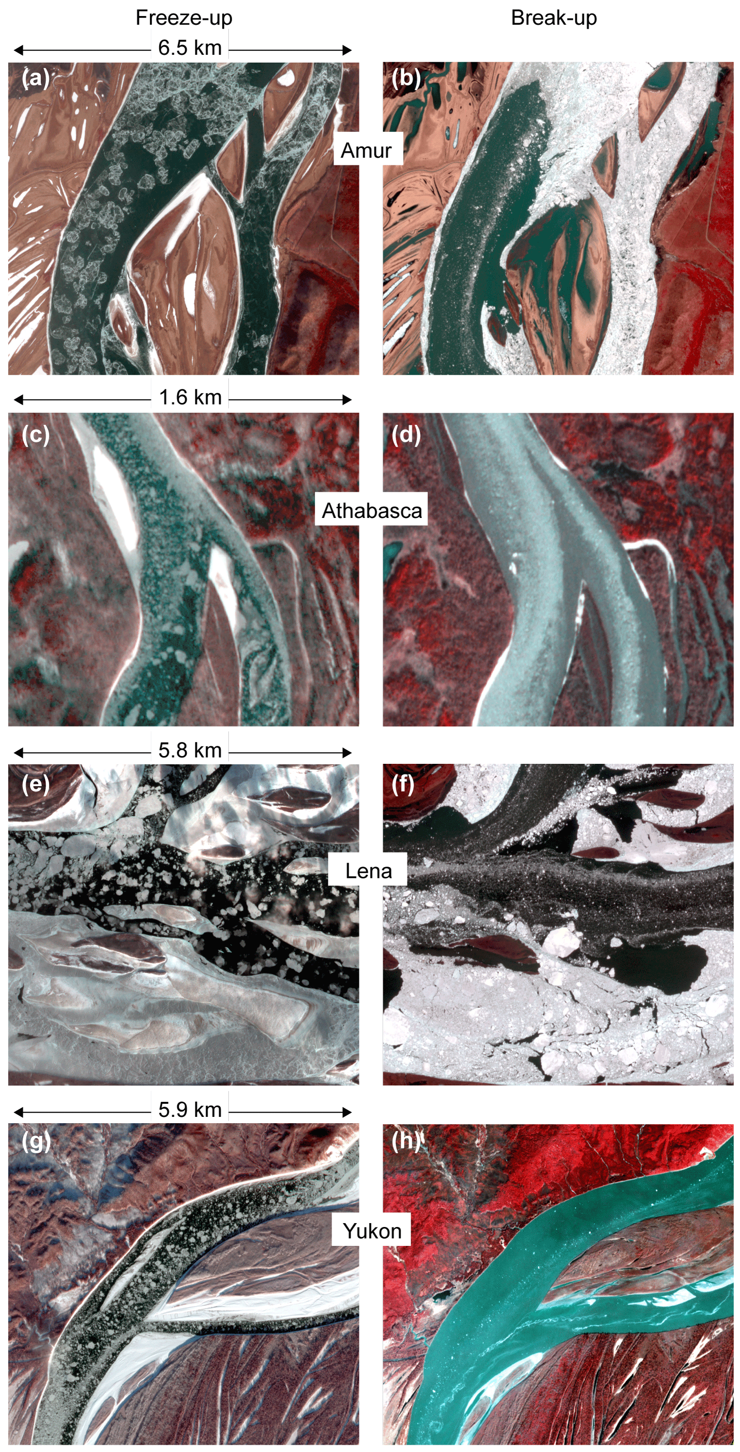
Figure 4Typical river-ice conditions in Planet imagery (shown in infrared false colour) that are suitable for tracking ice floes to estimate water velocities. (a, c, e, g) During freeze-up; (b, d, f, h) during break-up.
4.2 Amur River, Siberia
For a first example of river-ice velocities retrieved from near-simultaneous Planet cubesat images, we mosaic two respective overlapping sets of 12 scenes into two image strips covering an approximately 60 km long reach of the Amur River near the city of Komsomolsk-on-Amur in eastern Siberia. The image strip pair was acquired on 1 November 2016 (∼22:46 UTC) from an International Space Station (ISS) orbit, with a 73 s time lag. Figure 5a shows one of the two image strips as an infrared false colour composite. The freeze-up river-ice conditions during the acquisition were close to perfect for matching velocities. Ice floes densely covered most of the water surface, but were concurrently not colliding with each other in most areas; thus, the ice-floe velocities should to a large extent indicate water velocities at their locations. Ice-floe collisions would transfer additional lateral forces that overly the downstream drag by the river flow. Ice conditions on 1 November 2016 are shown in Fig. 6a. The diameter of visible ice floes generally ranges from around one pixel (3 m) to roughly 100 m, with a number of individual floes reaching up to 200–300 m. Figure 5b shows the magnitudes of the velocities derived, with maximum speeds of 1.7 m s−1 close to the lowest elevation of the river reach investigated (right margin of Fig. 5b). The displacement measurements were carried out within a manually digitized polygon roughly delineating the river floodplain around the river. The same correlation threshold of 0.7 was applied to all measurements, both on the river and outside. Successful displacements (i.e. measurements that passed the correlation threshold) are dense on the river but sparse on the floodplain surrounding the river, as the surface there seems to consist mostly of homogenous shrubs that offer little visual contrast to match at the 3 m image resolution. The images used in this example over Amur River stem from an early generation of Planet cubesats providing images with lower radiometric contrast compared with images from the current Planet cubesats (see Sect. 2). In addition, the contrast is reduced by the low sun angle during the acquisition. Despite these two complications, matches of ice floes seem robust, with the accuracy and reliability affected little, as the bright floes offer particularly strong visual contrast against the surrounding dark water surface. In summary, on the one hand, the sparse displacements surrounding the river (scattered blue results in Fig. 5) reflect the lack of good visual contrast to match between the two images on the floodplain. On the other hand, the small magnitude of these sparse displacements confirms that the two images co-register well. Figure 6 shows the original velocity vectors measured in more detail (rectangle in Fig. 5). The grid spacing of the vectors is 75 m.
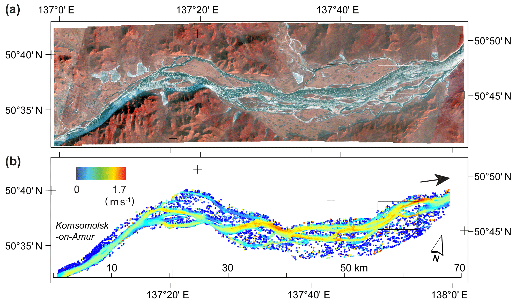
Figure 5Amur River near the city of Komsomolsk-on-Amur, Siberia (lower left corner). River surface velocities on 1 November 2016 are tracked over a 73 s time lag between overlapping Planet cubesat images. (a) A false colour composite of one of the image strips, and (b) the derived surface speeds. The overall flow direction is from left to right. The small rectangle marks the location of the detailed image shown in Fig. 6.

Figure 6Detailed zoom-in of a section of Fig. 5 (see small rectangle in Fig. 5). (a) Planet cubesat image from 1 November 2016, and (b) the original matched surface velocities after the constraint of the correlation coefficient. The grid spacing of vectors is 75 m. Matching results are given with the speed colour-coded and with velocity vectors superimposed. The maximum speed was 1.7 m s−1.
Figure 7 presents the longitudinal profile of speeds for the 1 November 2016 data set as well as the river width, which was automatically derived from the velocity vectors. Furthermore, we also compute the 2-D surface area flux as a function of transverse velocity profiles. As an example for the interpretation of the longitudinal profile, at approximately 25 km the 2-D surface area flux is relatively low, suggesting under mass conservation that the Amur River should be relatively deep at this part of the reach. In contrast, the river should be relatively shallow on average at, for instance, roughly 55 km. Interpretation of the longitudinal profile is influenced by the multi-branch geomorphology of the Amur River reach studied. In the individual speed measurements (grey dots in Fig. 7) branches become expressed by clusters of different speeds at the same reach section. For instance, at approximately 15–20 km, speeds on one branch are around 0.7 m s−1, whereas on the other branch they are up to 1.2 m s−1. Two clusters with different mean speeds on different branches are also clearly visible at around 30 km.
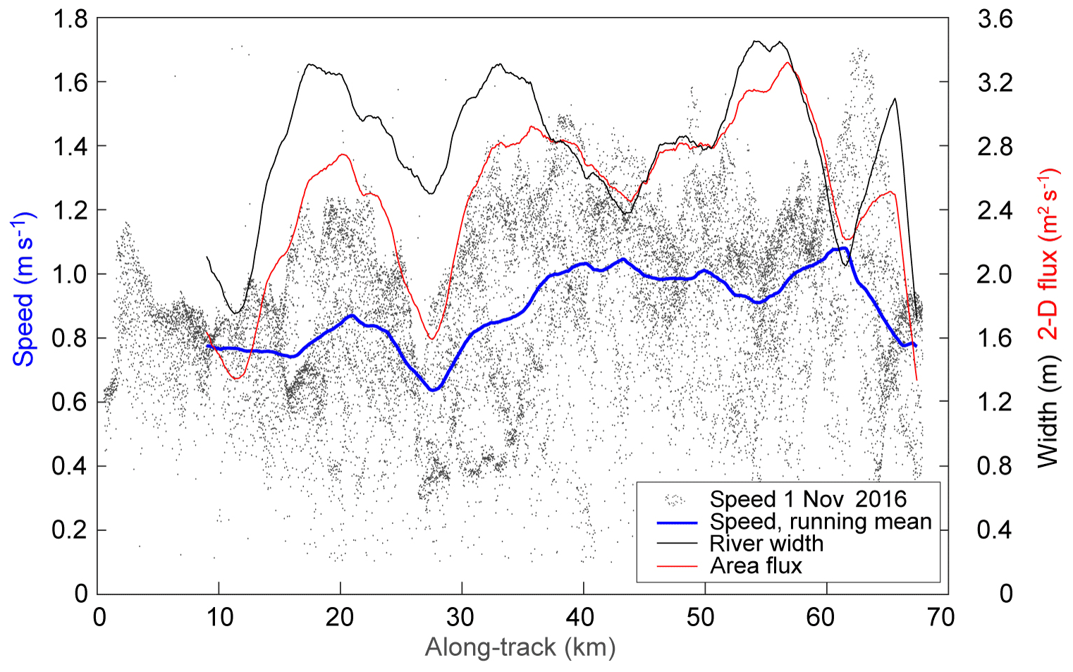
Figure 7Longitudinal profile of mean speeds and river widths derived from near-simultaneous Planet cubesat images from 1 November 2016 over a reach of the Amur River (Fig. 5). Small dots represent individual speed measurements; the blue line represents the 4 km running mean of individual measurements; the black line represents the river width from velocities (running mean); the red line represents the surface area flux as a product of cross-sectional average speed and river width (running mean).
4.3 Yukon River, Alaska
For a second case study we chose an approximate 200 km long reach of the Yukon River in Alaska (Fig. 8). Over this reach, the overall river azimuth coincides with the azimuth of the near-polar descending orbit of the Planet cubesats. We mosaic respective sequences of around 25 scenes to obtain two image strips for 16 May 2017 (∼21:12 UTC) with a 15 s time lag, and two images strips for 4 November 2018 (∼21:30 UTC) with a 171 s time lag. Typical ice conditions for these acquisitions are demonstrated in Fig. 4h and g respectively. The diameter of visible ice floes on the 4 November 2018 images ranges from around one pixel (3 m) to 100 m or more. There are many large ice floes of up to around 100 m in diameter. Larger ice floes of up to around 200 m can be found but are less frequent than on the Amur River images (Sect. 4.2). For 16 May 2017, the ice-floe diameters are significantly smaller and typically do not exceed a few pixels. The velocity magnitudes derived are shown in Fig. 8c and e, speed differences between them are shown in Fig. 8d, and details of these three items are displayed in Fig. 9. For comparison to a method that was used earlier, we add river-ice speeds derived for 13 May 2014 from a strip of ASTER stereo pairs (i.e. 55 s time lag) following the method by Kääb et al. (2013) and compute differences to the 16 May 2017 Planet data set (Fig. 8a, b). On 13 May 2014, river-ice cover was comparably sparse and subsequently so was the density of successful velocity matches. The freeze-up conditions on 4 November 2018 clearly offered the most complete cover by river-ice floes and, thus, the most complete velocity field. The river outlines used in Figs. 8 and 9 were obtained from a Landsat scene from 16 September 2013 as described in Sect. 3. Visually, these outlines represent the actual outlines from May 2014 and May 2017 very well, without significant changes over time. At shallow river sections, outlines from November 2018 (i.e. low water conditions) were, of course, more narrow than for September 2013. However, the outlines produced here are only used for visualization and the initial result segmentation into the “river” and “outside river” classes for accuracy assessment on stable ground.
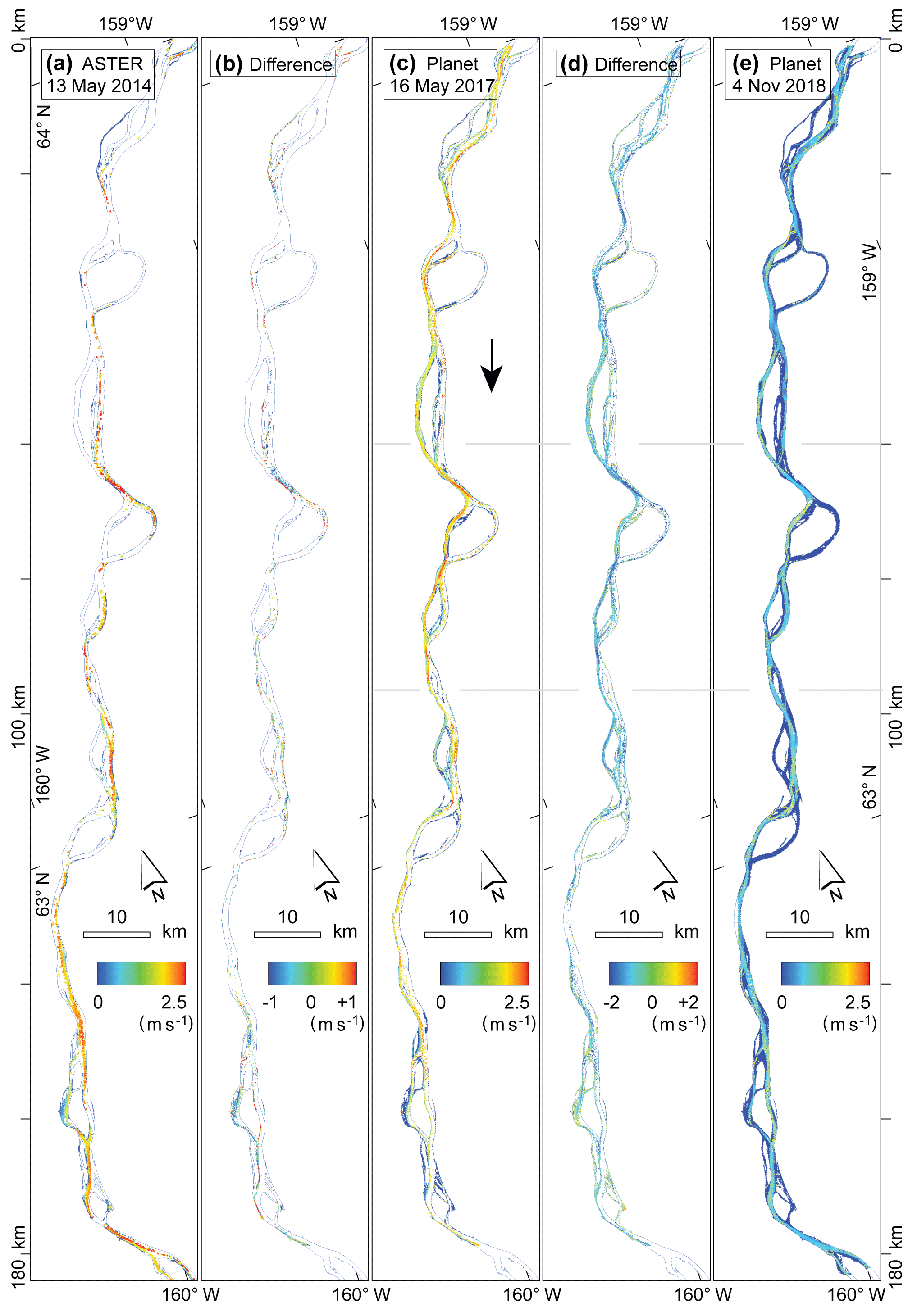
Figure 8Surface velocities on the Yukon River, Alaska, from near-simultaneous satellite images. The flow direction is roughly from north to south (top to bottom of the figure). Velocities from (a) an ASTER stereo pair from 13 May 2014 (55 s time lag), (c) two Planet cubesat image strips from 16 May 2017 (15 s), and (e) two Planet cubesat image strips from 4 November 2018 (171 s). Panels (b) and (d) show the differences between (c) and (a) and the differences between (e) and (c) respectively. The horizontal grey lines in (c–e) indicate the detail shown in Fig. 9.
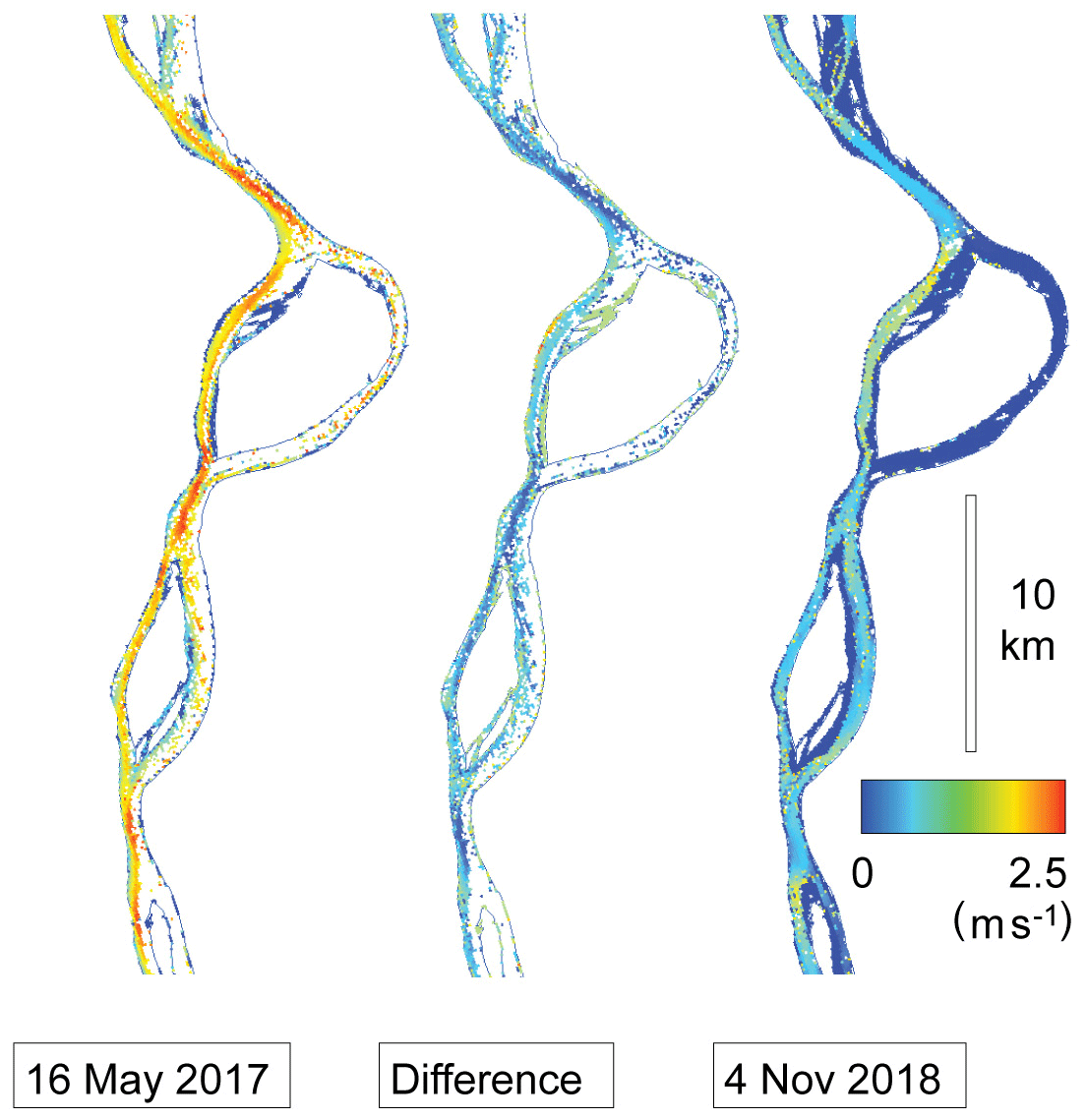
Figure 9Detail of water surface velocities shown in Fig. 8. For more information see the caption of Fig. 8.
The closest river discharge measurements to the Yukon River reach used in this study are carried out at Pilot Station (no. 15565447), some 300 km downstream of the lower end of the reach studied. For 13 May 2014, 16 May 2017, and 4 November 2018 discharge estimates at Pilot Station are 11 383, 8410, and 5437 m3 s−1 respectively. Taking the distance between the reach investigated and Pilot Station into account, we also give the discharges 3 d later: 13 450, 11 213, and 4927 m3 s−1 for 16 May 2014, 19 May 2017, and 7 November 2018 respectively. Similar to the discharges, the surface velocities measured for 13 May 2014 are also higher than for 16 May 2017, and the latter values are higher than for 4 November 2018, as can be seen from Fig. 8b and d. The mean speed on 4 November 2018 is 0.80, whereas it is 1.35 m3 s−1 on 16 May 2017. Due to the sparse coverage by successful measurements in the ASTER data (Fig. 8a), only a few differences can be computed to the Planet data (Fig. 8b). The differences between the two Planet data sets (Fig. 8d) are much denser, demonstrating the advantage of the high-resolution Planet cubesat data in combination with the denser coverage by ice floes during the freeze-up. Speeds between 19 May 2017 and 7 November 2018 vary both with respect to the longitudinal average (Fig. 10b) and across the river (Figs. 8d, 9). In future applications, these measured spatio-temporal variations of surface water speed could be analysed in combination with known bathymetry and/or hydraulic formulae.

Figure 10The longitudinal profile of speeds and river widths derived from near-simultaneous Planet cubesat images. (a) Measurements from 4 November 2018. Small dots represent the individual speed measurements; the blue line represents the 4 km running mean of individual measurements; the black line represents the river width from velocities (running mean); the red line is the surface area flux as a product of the cross-sectional average speed and river width (running mean). (b) The running means of surface speeds and the river width for 4 November 2018 (dark blue and black respectively) and 16 May 2017 (light blue and grey respectively). (c) Indicators of result quality. Small dots are speeds on stable ground for 4 November 2018, i.e. outside of the river. The green and turquoise lines are the percentage of successful measurements (i.e. measurements passing the correlation coefficient threshold) compared to the complete river mask. Blue and light blue lines in (c) are the speeds as in (b).
Figure 10a shows the longitudinal profile of speeds for the 4 November 2018 data set and the river width automatically derived from the velocity vectors. Furthermore, we also compute the 2-D surface flux as a function of the transverse velocity profiles. As an example for interpretation of the longitudinal profile, at approximately 80 km, the 2-D surface flux is relatively low, suggesting under mass conservation that the Yukon River should be relatively deep at this part of the reach. In contrast, the river should be relatively shallow at on average, for instance, approximately 120 km.
From a similar profile of river surface speed along 400 km of the Lena River on 27 May 2011, Kääb et al. (2013) found a striking peak in the power spectrum of the river surface speed at 20.8 km. For the Yukon River profile in Fig. 10, we find a somewhat less prominent but still significant peak in the power spectrum of speeds at 20.5 km. The similar number for both river reaches might point to similar processes and parameters for the development of the respective river morphologies (Lanzoni, 2000a, b). Kääb et al. (2013) provide an additional discussion on the 20.8 km wavelength speed variations including comparison to a topographic profile.
The profile in Fig. 10b compares river surface speeds and river widths on 16 May 2017 and 4 November 2018. The four data sets are consistent in the sense of mass conservation: higher discharges in May 2017 compared to November 2018 (see above discharges for Pilot Station) correspond to a combination of larger widths and higher surface speeds. For instance, at sections where the river width is significantly larger in May 2017 than in November 2018, speed differences between May 2017 and November 2018 are smaller (e.g. at roughly 60, 110, or 170 km). Conversely, at sections with relatively small changes in river width, surface speeds change more (e.g. at roughly 30, 90, or 130 km).
4.4 Error budget
The error budget for individual river surface velocity measurements consists of three main components: (i) offsets in the absolute georeference of a set of repeat images, (ii) relative distortions and offsets between repeat images, and (iii) errors from the matching of features between the repeat images. The first category, the uncertainty of the absolute georeference, mostly stems from matching the Planet images onto a reference image. This step is part of the Planet in-house processing and is, in our experience, typically accurate to approximately one pixel or less, but can be larger for partially cloud-covered or snow-covered scenes. Failure or gross uncertainties of this georeference refinement step and subsequent gross georeference errors are flagged by Planet in the image metadata. To the best of our knowledge, an absolute georeference accuracy of a few metres or pixels for the locations of the velocities derived should not be a problem for most applications, in particular when considering that the velocities derived represent a window of several tens of metres (here 90 m × 90 m). The second category of uncertainty, the distortions and offsets between the images matched, can be minimized by co-registration, which is typically possible with sub-pixel accuracy. This uncertainty source is not necessarily eliminated for small-scale higher-order distortions (see Sect. 3) that differ between the stable ground used for co-registration (river shore, flood plain, etc.) and the actual river surface. The parts of this second error component that are not eliminated by image co-registration mix with the third error category, which is the actual matching accuracy for the respective stable ground or river-ice features. This relative matching accuracy between existing co-registered images defines the uncertainty of the actual displacements or velocities derived; thus, here we consider it as the error component of largest interest (Kääb et al., 2013) and focus on it in more detail in the following.
Uncertainties of individual velocity measurements or outliers (our above error component iii) stem from uncertainties in the definition of river-ice features over time, i.e. how sharply features that change over time can be matched and how (precisely) is a displacement between slightly modified features defined. This error component includes the representativeness of displacements matched using a 90 m × 90 m window for actual point-wise velocities, and the degradation of the matching accuracy by rotation or deformation of river-ice features over the minute-scale time lag exploited here (Kääb et al., 2013). We estimate the accuracy of our river-ice velocity measurements in the following three ways: (1) inference from previous studies, (2) stable ground matches, and (3) variance of velocities within homogenous parts of the derived flow field.
-
Based on ASTER data over the Lena river, Kääb et al. (2013) suggest a displacement accuracy of up to one-eighth of a pixel for most optimal imaging and ice conditions, which, in our case, would translate to about 0.4–0.5 m (or 0.005 m s−1 for a 90 s time lag).
-
Based on about 27 000 matches on the floodplains around the rivers investigated in this study we obtain a mean displacement dx of m, a dy of m, and a mean displacement length (Pythagoras of individual dx and dy) of 0.4±0.6 m. Besides a good co-registration accuracy of around 0.2 m (i.e. about 1∕15 of a pixel), our stable ground tests suggest an accuracy of the individual velocity measurements of ±0.6 m (one-fifth of a pixel; 0.007 m s−1 for 90 s). This latter number agrees well with the accuracy estimates for co-seismic displacement measurements from repeat Planet data of one-fourth of a pixel (Kääb et al., 2017). Figure 10c shows a longitudinal profile of stable ground matches (in m s−1; black dots) for the 4 November 2018 data. The stable ground median speed is 0.02 m s−1, and the mean is 0.03 m s−1. Similar results are found for 16 May 2017. These values can be considered an upper limit for the accuracy of ice-floe measurements as the river ice floes offer better visual contrast for the matching than the areas surrounding the river (see Sect. 4.2), and the image areas outside of the river are likely subject to larger topographic distortions than the river surface (see Sect. 3).
-
Variations of velocities within the homogenous parts of the derived flow fields, i.e. the standard deviation of means over such parts of the flow fields, range between ±0.3 m in our tests for the shortest time lag in our study (15 s; translating to 0.02 m s−1) and ±3 m for our longest time lag (171 s; 0.02 m s−1). Especially for the longer time lags, deformations of the river-ice features matched and rotations of individual ice floes certainly degrade the actual matching accuracy.
From our above three approaches, as a rule of thumb, we suggest an accuracy of the order of ±0.01 m s−1 for individual river-ice velocities derived from near-simultaneous PlanetScope data. Note that this accuracy improves following standard error propagation rules, once individual velocities are averaged, for instance for cross-sectional or longitudinal means.
As another possible indicator of measurement quality, Fig. 10c shows the percentage of successful matches on the river. Clearly, this percentage is much higher for the 4 November 2018 freeze-up conditions than for the 16 May 2017 break-up conditions on the Yukon River. This indicator can be used in several ways, for instance for masking out the results for reach sections with low values, for developing weighting of the above nominal accuracy, or for analysing unwanted dependencies between results and measurement density. The stable ground matches (dots in Fig. 10c) also exhibit errors in co-registration. For the 4 November 2018 data, a small co-registration problem can be seen at about 140–160 km with elevated speeds. Kääb et al. (2013) demonstrate a procedure to correct such offsets.
In this study, we exploit the fact that the cross-track overlaps of the swaths of subsequent PlanetScope cubesats (Figs. 2 and 3) produce near-simultaneous optical acquisitions, separated by approximately 90 s. Over this time lag we track river ice floes and use them as indicators for water surface velocities. Planet cubesats scan the entire land surface of the Earth at daily repeat and with an approximate 3 m spatial image resolution. Our study shows that these data substantially extend the possibilities to measure river-ice and water surface flow from near-simultaneous optical satellite data. Over many rivers that carry river ice, ice floes can be tracked during freeze-up and/or break-up with accuracies of the order of ±0.01 m s−1. Freeze-up conditions appear to be particularly well suited for this work due to the longer time periods over which ice floes are present, and the more favourable types and densities of ice floes.
We find three main obstacles when applying the method. By constellation design, the PlanetScope cross-track overlaps (never intended for measuring minute-scale changes and motions!) do not cover the entire Earth surface but only parts of it, depending on latitude, for instance two-thirds of a cubesat swath at 65∘ N (Fig. 3). Second, cloud cover seems rather typical for the river freeze-up and break-up seasons, and considerably complicates the acquisition of suitable Planet cubesat data – as for any optical satellite instrument. Third, freeze-up for some of the northernmost rivers or river reaches seems to occur during sun angles that are too low to acquire suitable images. As a very rough guess from our Planet cubesat archive searches, we estimate that there is a 50 % chance of getting a least one cubesat image per year with drifting ice visible for a given river location. The chances that the river location is then included in the swath overlap from a subsequent cubesat is lower, and the chances are considerably lower again when considering river locations that are covered several times (per year or in total) by overlaps that enable tracking. However, despite these limitations, the tracking of river ice in near-simultaneous Planet cubesat data substantially increases the possibilities for deriving surface velocities on cold-region rivers compared with the very few occasional optical stereo acquisitions suitable for the same purpose.
The strong visual contrast provided by the bright ice floes on the dark water surface, in combination with the short time lag of around 1 min exploited here, lead to few other motion components apart from translation and represent quite optimal conditions for image matching. Therefore, as our study is focused on evaluating the potential of the Planet cubesat constellation, not on the image matching algorithm, we used standard normalized cross-correlation (NCC) as the tracking method. Future work could test if other tracking methods have advantages over NCC for tracking ice floes in near-simultaneous satellite images. In particular for sea-ice tracking, other matching procedures are used that are optimized to work on sequences of low-resolution satellite data with time lags of hours to days (e.g. Lavergne et al., 2010; Petrou and Tian, 2017). An overview and assessment of state-of-the-art image-based tracking approaches for water flow measurements, in which some are certainly relevant for near-simultaneous Planet cubesat data, is given in Lin et al. (2019).
The parameters provisionally chosen for the moving windows to compute longitudinal flow averages (4 km length, 100 m step width) could easily be adjusted. Our visualizations turn out to be little sensitive to the exact choice of window parameter values. For the long river reaches studied here, the mean river direction defining the initial window orientations is almost identical to the orbit azimuth. Thus, the image matches on the floodplain outside the rivers can easily be transformed into their satellite along-track and cross-track components, which is a preferred coordinate system for analysing the geometric performance and errors in satellite data (Kääb et al., 2013). In the present study we do not find geometric errors of concern, such as satellite jitter, which Kääb et al. (2013) found and corrected in a similar study based on another satellite data type.
As we only use our longitudinal averaging procedure for visualization purposes, it is not optimized for specific applications such as estimating river width, discharge, or parameters of river morphology and flow. In particular, larger voids in the measured velocity field, due to low correlation coefficients, will bias the flow averages per window step. This effect seems strongly reduced for freeze-up conditions as the coverage by ice floes during these conditions typically appears to be much more complete compared with break-up conditions (see Sect. 4.1). River areas without ice floes only lead to voids in the measurements if they are larger than the matching window size (here 30 pixels ×30 pixels; 90 m × 90 m) in at least one dimension, as the matching algorithm used (NCC) is not sensitive to where the matched features are located in the window. A first measure to indicate problems from voids in the velocity field in the profiles is to plot the percentage of void pixels per window position (Fig. 10c). Smaller voids can be filled, whereby the measured velocities enable the application of a directional interpolator, or the matching window sizes can be automatically adapted to the distribution of ice floes – small windows for dense ice floes and larger ones for sparse ice floes (Debella-Gilo and Kääb, 2011a). The effect of voids on derived parameters can be tested by simulating voids for a rather complete data set (e.g. the Yukon River 4 November 2018) from actual voids in another data set (e.g. the Yukon River 16 May 2017) (McNabb et al., 2019).
Another effect to be taken into account is the influence of river branching on the averages. Again, treatment of this effect depends much on application and parameters of interest. For instance, the mean flow speed and surface area flux that we compute are not affected, whereas making connections between our surface flow measurements and river discharge would require taking branching into account. An initial simple procedure for that purpose would be to intersect the moving window at each step with the river outlines and to compute the flow averages for each intersection area separately.
Although not exploited further in this study, we would like to note the existence of a Sentinel-2 scene of 4 November 2018, taken about 1 h after the Planet scenes over Yukon River. Due to this large time lag between the Planet and Sentinel-2 scenes and the related large displacements and deformations/rotations of river-ice features, traditional image matching methods that solve only for translations are complicated, but manual tracking of distinct floes is still clearly possible. Tests show good agreement between the speeds derived over 1 h and those over 171 s. Thus, the fact that most Planet cubesats, Sentinel-2A and 2B, and Landsat 7 and 8 are on similar orbits can create additional opportunities for tracking river-ice movement, for investigating short-term changes in river-ice cover and speed, and for additional or combined multispectral mapping and analysis in combination with the Planet cubesats.
As demonstrated here for a 200 km long reach of the Yukon River, remotely-sensed water velocities over long reaches might offer improved insights into river morphology. For instance, we find a variation in water speeds of approximately 20–21 km wavelength for the Yukon River (and the Lena River; Kääb et al., 2013) that could be compared to according wavelengths found from laboratory experiments and models on bar formation (Lanzoni, 2000a, b).
A major purpose of satellite-based river observations is to estimate discharge in order to spatially or temporally complement the sparse in situ measurements available from gauging stations (Beltaos and Kääb, 2014; Bjerklie et al., 2018; Zakharova et al., 2019; and many others, see references in the cited ones). River velocities from the approach demonstrated here can offer an additional type of input measurement (or a possibility for independent comparison) when linking satellite-based measurements of river height and slope from altimetry data, and measurement of river surface from optical (Allen and Pavelsky, 2018) or radar images, to standard discharge equations (Bjerklie et al., 2018; Zakharova et al., 2019). Such satellite data are available over large regions (Allen and Pavelsky, 2018) and consequently fit well to the river velocities as derived by our approach. Satellite-altimetric river heights will even improve in the (near) future due to the new Sentinel-3 and high-resolution ICESat-2 missions (Brown, 2019), and the upcoming SWOT mission (Durand et al., 2010). Moreover, Landsat 8 and Sentinel-2 combined offer sub-weekly repeat to measure parameters such as river width.
In summary, the water mapping opportunities from the daily repeat Planet data (Cooley et al., 2017) and opportunities to measure ice velocities from them, as demonstrated here, could aid in detecting ice jams and related flooding (Fig. 1), as well as providing a better understanding of the mechanisms involved in ice jam formation. The damages from ice jam floods cause annual economic losses of the order of several hundred million EUR per year in North America and Siberia (Prowse et al., 2007; Rokaya et al., 2018a, b). Finally, while substantially fewer in number, we speculate that near-simultaneous overpasses of tropical and temperate rivers could similarly be exploited, tracking sediment or floating matter in place of ice (Kääb and Leprince, 2014).
The image matching code used for this study (Correlation Image AnalysiS, CIAS) is available from http://www.mn.uio.no/icemass (Kääb, 2014).
Sentinel-2 data are freely available from the ESA/EC Copernicus Sentinels Scientific Data Hub at https://scihub.copernicus.eu/ (Copernicus Open Access Hub, 2019); Landsat 8 data are available from USGS at http://earthexplorer.usgs.gov/ (USGS EarthExplorer, 2019); ASTER data are available from https://earthdata.nasa.gov/ (NASA Earthdata, 2019); Yukon River discharge data are available from https://waterdata.usgs.gov (USGS Waterdata, 2019). Planet data are not openly available as Planet is a commercial company; however, scientific access schemes to these data exist (https://www.planet.com/markets/education-and-research/).
AK developed the study, carried out most of the analyses, and wrote the paper. BA supported the analyses and edited the paper. JM helped with data acquisition, contributed technical details regarding the Planet constellation and data, and edited the paper.
AK and BA declare that they have no competing interests. JM was programme manager for impact initiatives at Planet. He in no way influenced the results or conclusions of the study.
Special thanks are due to two anonymous referees for their detailed and constructive comments, and to the editor of this paper. We are grateful to the data providers for this study: Planet for their cubesat data via the Planet's Ambassadors Program, ESA/Copernicus for the Sentinel-2 data, USGS for the Landsat 8 and river discharge data, and NASA and the ASTER science team at JPL for the ASTER data. Special thanks are due to Michael Abrams for tasking the May 2014 ASTER acquisitions over the Yukon River. This work was funded by the European Research Council under the European Union's Seventh Framework Programme, the ESA project Glaciers_cci, the ESA Living Planet Fellowship to Bas Altena, and the ESA EarthExplorer10 Mission Advisory Group.
This research has been supported by the European Research Council (project: FP/2007-2013/ERC; grant no. 32081) and the European Space Agency (projects: 4000125560/18/I-NS and 4000109873/14/I-NB).
This paper was edited by Bettina Schaefli and reviewed by two anonymous referees.
Allen, G. H. and Pavelsky, T. M.: Global extent of rivers and streams, Science, 361, 585–587, https://doi.org/10.1126/science.aat0636, 2018.
Altena, B. and Kääb, A.: Elevation change and improved velocity retrieval using orthorectified optical satellite data from different orbits, Remote. Sens.-Basel, 9, 300, https://doi.org/10.3390/rs9030300, 2017.
Beltaos, S. and Kääb, A.: Estimating river discharge during ice breakup from near-simultaneous satellite imagery, Cold Reg. Sci. Technol., 98, 35–46, https://doi.org/10.1016/j.coldregions.2013.10.010, 2014.
Bjerklie, D. M., Birkett, C. M., Jones, J. W., Carabajal, C., Rover, J. A., Fulton, J. W., and Garambois, P. A.: Satellite remote sensing estimation of river discharge: Application to the Yukon River Alaska, J. Hydrol., 561, 1000–1018, https://doi.org/10.1016/j.jhydrol.2018.04.005, 2018.
Brown, M.: Ice, Cloud, and Land Elevation Satellite-2 (ICESat-2) Applications: Monitoring Fresh Water Availability, available at: https://icesat-2.gsfc.nasa.gov/sites/default/files/ICESat-2_InlandWater_Whitepaper_040116.pdf, last access: 10 July 2019.
Cooley, S. W., Smith, L. C., Stepan, L., and Mascaro, J.: Tracking dynamic northern surface water changes with high-frequency Planet cubesat imagery, Remote Sens.-Basel, 9, 1306, https://doi.org/10.3390/rs9121306, 2017.
Copernicus Open Access Hub: Copernicus programme, European Commission and European Space Agency, available at: https://scihub.copernicus.eu, last access: 17 October 2019.
d'Angelo, P., Kuschk, G., and Reinartz, P.: Evaluation of Skybox Video and Still Image Products, Int. Arch. Photogram., XL-1, 95–99, https://doi.org/10.5194/isprsarchives-XL-1-95-2014, 2014.
d'Angelo, P., Mattyus, G., and Reinartz, P.: Skybox image and video product evaluation, Int. J. Image Data Fus., 7, 3–18, https://doi.org/10.1080/19479832.2015.1109565, 2016.
Debella-Gilo, M. and Kääb, A.: Locally adaptive template sizes in matching repeat images of Earth surface mass movements, ISPRS J. Photogram., 69, 10–28, https://doi.org/10.1016/j.rse.2010.08.012, 2011a.
Debella-Gilo, M. and Kääb, A.: Sub-pixel precision image matching for measuring surface displacements on mass movements using normalized cross-correlation, Remote Sens. Environ., 115, 130–142, https://doi.org/10.1016/j.rse.2010.08.012, 2011b.
Debella-Gilo, M. and Kääb, A.: Measurement of surface displacement and deformation of mass movements using least squares matching of repeat high resolution satellite and aerial images, Remote Sens.-Basel, 4, 43–67, https://doi.org/10.3390/rs4010043, 2012.
Drusch, M., Del Bello, U., Carlier, S., Colin, O., Fernandez, V., Gascon, F., Hoersch, B., Isola, C., Laberinti, P., Martimort, P., Meygret, A., Spoto, F., Sy, O., Marchese, F., and Bargellini, P.: Sentinel-2: ESA's optical high-resolution mission for GMES operational services, Remote Sens. Environ., 120, 25–36, https://doi.org/10.1016/j.rse.2011.11.026, 2012.
Durand, M., Rodriguez, E., Alsdorf, D. E., and Trigg, M.: Estimating river depth from remote sensing swath interferometry measurements of river height, slope, and width, IEEE J.-Stars, 3, 20–31, https://doi.org/10.1109/Jstars.2009.2033453, 2010.
Foster, C., Hallam, H., and Mason, J.: Orbit determination and differential-drag control of Planet Labs cubesat constellation, in: AIAA Astrodynamics Specialist Conference, August 2015, Vale, CO, available at: https://arxiv.org/pdf/1509.03270.pdf (last access: 17 October 2019), 2015.
Girod, L., Nuth, C., and Kääb, A.: Improvemement of DEM generation from ASTER images using satellite jitter estimation and open source implementation, Int. Arch. Photogramm. Remote Sens. Spatial Inf. Sci., XL-1/W5, 249–253, https://doi.org/10.5194/isprsarchives-XL-1-W5-249-2015, 2015.
Heid, T. and Kääb, A.: Evaluation of existing image matching methods for deriving glacier surface displacements globally from optical satellite imagery, Remote Sens. Environ., 118, 339–355, https://doi.org/10.1016/j.rse.2011.11.024, 2012.
Kääb, A.: Correlation Image Analysis software (CIAS), available at: http://www.mn.uio.no/icemass (last access: 10 July 2019), 2014.
Kääb, A. and Leprince, S.: Motion detection using near-simultaneous satellite acquisitions, Remote Sens. Environ., 154, 164–179, https://doi.org/10.1016/j.rse.2014.08.015, 2014.
Kääb, A. and Prowse, T.: Cold-regions river flow observed from space, Geophys. Res. Lett., 38, L08403, https://doi.org/10.1029/2011GL047022, 2011.
Kääb, A. and Vollmer, M.: Surface geometry, thickness changes and flow fields on creeping mountain permafrost: automatic extraction by digital image analysis, Permafrost Periglac., 11, 315–326, https://doi.org/10.1002/1099-1530(200012)11:4<315::Aid-Ppp365>3.0.Co;2-J, 2000.
Kääb, A., Lamare, M., and Abrams, M.: River ice flux and water velocities along a 600 km-long reach of Lena River, Siberia, from satellite stereo, Hydrol. Earth Syst. Sci., 17, 4671–4683, https://doi.org/10.5194/hess-17-4671-2013, 2013.
Kääb, A., Winsvold, S. H., Altena, B., Nuth, C., Nagler, T., and Wuite, J.: Glacier remote sensing using Sentinel-2. Part I: radiometric and geometric performance, and application to ice velocity, Remote Sens., 8, 598–622, https://doi.org/10.3390/Rs8070598, 2016.
Kääb, A., Altena, B., and Mascaro, J.: Coseismic displacements of the 14 November 2016 Mw 7.8 Kaikoura, New Zealand, earthquake using the Planet optical cubesat constellation, Nat. Hazards Earth Syst. Sci., 17, 627–639, https://doi.org/10.5194/nhess-17-627-2017, 2017.
Lanzoni, S.: Experiments on bar formation in a straight flume 1. Uniform sediment, Water Resour. Res., 36, 3337–3349, https://doi.org/10.1029/2000wr900160, 2000a.
Lanzoni, S.: Experiments on bar formation in a straight flume 2. Graded sediment, Water Resour. Res., 36, 3351–3363, https://doi.org/10.1029/2000wr900161, 2000b.
Lavergne, T., Eastwood, S., Teffah, Z., Schyberg, H., and Breivik, L. A.: Sea ice motion from low-resolution satellite sensors: An alternative method and its validation in the Arctic, J. Geophys. Res.-Oceans, 115, C10032, https://doi.org/10.1029/2009jc005958, 2010.
Lin, D., Grundmann, J., and Eltner, A.: Evaluating image tracking approaches for surface velocimetry with thermal tracers, Water Resour. Res., 55, 3122–3136, https://doi.org/10.1029/2018wr024507, 2019.
McFeeters, S. K.: The use of the normalized difference water index (NDWI) in the delineation of open water features, Int. J. Remote Sens., 17, 1425–1432, https://doi.org/10.1080/01431169608948714, 1996.
McNabb, R., Nuth, C., Kaab, A., and Girod, L.: Sensitivity of glacier volume change estimation to DEM void interpolation, The Cryosphere, 13, 895–910, https://doi.org/10.5194/tc-13-895-2019, 2019.
NASA Earthdata: National Air and Space Administration Earthdata, available at: https://earthdata.nasa.gov/, last access: 17 October 2019.
Nuth, C, and Kääb, A.: Co-registration and bias corrections of satellite elevation data sets for quantifying glacier thickness change, The Cryosphere, 5, 271–290, https://doi.org/10.5194/tc-5-271-2011, 2011.
Paul, F., Kääb, A., Maisch, M., Kellenberger, T., and Haeberli, W.: The new remote-sensing-derived Swiss glacier inventory: I. Methods, Ann. Glaciol., 34, 355–361, https://doi.org/10.3189/172756402781817941, 2002.
Pekel, J. F., Cottam, A., Gorelick, N., and Belward, A. S.: High-resolution mapping of global surface water and its long-term changes, Nature, 540, 418–422, https://doi.org/10.1038/nature20584, 2016.
Petrou, Z. I. and Tian, Y. L.: High-resolution sea ice motion estimation with optical flow using satellite spectroradiometer data, IEEE T. Geosci. Remote, 55, 1339–1350, https://doi.org/10.1109/Tgrs.2016.2622714, 2017.
Planet Application Program Interface: In Space for Life on Earth, San Francisco, CA, available at: https://api.planet.com/ and https://www.planet.com/, last access: 1 January 2019.
Prowse, T. D., Bonsal, B., Duguay, C. R., Hessen, D. O., and Vuglinsky, V. S.: River and lake ice, in: Global Outlook for Ice & Snow, United Nations Environment Programme, United Nations Environment Programme (UNEP), Nairobi, 201–214, 2007.
Rokaya, P., Budhathoki, S., and Lindenschmidt, K. E.: Trends in the timing and magnitude of ice-jam floods in Canada, Sci. Rep.-UK, 8, 5834, https://doi.org/10.1038/s41598-018-24057-z, 2018a.
Rokaya, P., Budhathoki, S., and Lindenschmidt, K. E.: Ice-jam flood research: a scoping review, Nat. Hazards, 94, 1439–1457, https://doi.org/10.1007/s11069-018-3455-0, 2018b.
Romeiser, R., Runge, H., Suchandt, S., Sprenger, J., Weilbeer, H., Sohrmann, A., and Stammer, D.: Current measurements in rivers by spaceborne along-track InSAR, IEEE T. Geosci. Remote, 45, 4019–4031, https://doi.org/10.1109/Tgrs.2007.904837, 2007.
USGS EarthExplorer: United States Geological Survey EarthExplorer, available at: https://earthexplorer.usgs.gov/, last access: 17 October 2019.
USGS Waterdata: United States Geological Survey, National Water Information System, available at: https://waterdata.usgs.gov, last access: 17 October 2019.
Zakharova, E. A., Krylenko, I. N., and Kouraev, A. V.: Use of non-polar orbiting satellite radar altimeters of the Jason series for estimation of river input to the Arctic Ocean, J. Hydrol., 568, 322–333, https://doi.org/10.1016/j.jhydrol.2018.10.068, 2019.